Simultaneously Estimation of Super-Resolution

Images and Depth Maps from

Low Resolution Sensors

Daniel B. Mesquita, Erickson R. Nascimento, Mario F. M. Campos

Computer Science Department

Universidade Federal de Minas Gerais

Belo Horizonte, MG, Brazil

E-mail: balbino,erickson,mario@dcc.ufmg.br

Abstract—The emergence of low cost sensors capable ofproviding texture and depth information of a scene is enablingthe deployment of several applications such as gesture andobject recognition and three-dimensional reconstruction of en-vironments. However, commercially available sensors output lowresolution data, which may not be suitable when more detailedinformation is necessary. With the purpose of increasing dataresolution, at the same time reducing noise and filling the holesin the depth maps, in this work we propose a method thatcombines depth fusion and image reconstruction in a super-resolution framework. By joining low-resolution intensity imagesand depth maps in an optimization process, our methodologycreates new images and depth maps of higher resolution and,at the same time, minimizes issues related with the absence ofinformation (holes) in the depth map. Our experiments showthat the proposed approach has increased the resolution of theimages and depth maps without significant spawning of artifacts.Considering three different evaluation metrics, our methodologyoutperformed other three techniques commonly used to increasethe resolution of combined images and depth maps acquired withlow resolution, commercially available sensors.

Keywords-Super-resolution, convex optimization, RGB-D data,3D reconstruction, computer vision.

I. INTRODUCTION

The increasing availability of low-cost sensors capable of

capturing both image and depth information, also known

as RGB-D sensors such as Kinect, opened a wide research

horizon for several methodologies involving processing of

geometry and visual data. If on one hand these sensors

can provide a good initial estimate of the three-dimensional

structure of the scene with texture embedded, on the other

hand such sensors provide low resolution images and noisy

depth maps. Since the results of several algorithms are directly

dependent on the quality and amount of detail present in

the data, sharpening images and depth maps can increase the

accuracies for object recognition and improve precision of 3D

alignment and reconstruction [1].

In general, a super-resolution method can be divided into

two main steps: registration and interpolation. The first step

consists of finding the transformation of the frames to the

same coordinate system (e.g. the coordinate system defined

by camera’s pose in the acquisition of the first image in the

sequence). The second step estimates the intensity information

of pixels for a larger grid.

When the sensor moves freely in the scene, matching

between pixels is usually performed by optical flow. However,

this approach has high computational cost and cannot be ap-

plied when sensor displacements are large. Therefore, several

techniques have been proposed to use depth information in

order to estimate pixel correspondences making the estima-

tion more efficient. Despite the quality provided by these

techniques, it is necessary to provide the depth information

and in most cases, image reconstruction methods are used

to estimate the depth. Although these strategies are able to

determine the correspondence, they use a depth map which is

a rough approximation of the real map. This limits the image

quality estimation, since such depth maps contain errors that

are propagated to the interpolation step.

The main contribution of this work is a new method for

3D reconstruction based on an optimization approach which

provides super-resolution intensity and depth images acquired

by a low resolution sensor, such as commercially available

RGB-D sensors. Our proposed model is defined as a convex

optimization problem for which state of the art optimization

techniques are employed to find the best solution.

This paper is structured as follows: Section II presents an

overview of the works in the area of super-resolution. Initially

we discuss the main works in the area of super-resolution for

intensity images, followed by a discussion on works that use

depth maps. Section III discusses the proposed approach: An

optimization method that uses three-dimensional reconstruc-

tion techniques for the fusion of images and depth maps to

generate high-resolution image results. Results are presented

and discussed in Section IV, starting with the validation of

our method using synthetic images followed by a quantitative

analysis and experiments with RGB-D data. Finally, Section

V sums up the conclusions attained with the development and

implementation of our methodology and indicates directions

for future research.

II. RELATED WORKS

In general, the methodologies for super-resolution may be

broadly divided into two main categories: Super-resolution

by example and reconstruction based super-resolution. While

methodologies in the former category use learning-based ap-

proaches in order to increase the resolution of images, in

the latter it is assumed as a basic premise that the low

resolution images (LR) are subsamples with subpixel precision

of some high resolution image (HR), and which can be used

to reconstruct the original HR image.

Thanks to the increasing access to devices capable of

obtaining geometrical data from the scene, several super-

resolution techniques have included the use of depth maps in

their approach. In [2] the authors proposed a method based

on MRF (Markov Random Fields) to integrate the depth

information acquired by a laser scanner with images from

a high resolution camera. A similar technique is presented

in [3]. By using a ToF (Time-of-flight) camera to acquire range

images and applying a bilateral filter, they present an iterative

algorithm to enlarge the spatial resolution of depth maps.

In [4], the problem of super-resolution is modeled by using

a calibrated three-dimensional scene and a probabilistic frame-

work based on MAP-MRF. Although their method efficiently

handles occlusions in the depth maps, the algorithm does not

estimate depth, which reduces the quality of their results in

regions which contain holes in the depth map. In [5], the

authors present a method for increasing the precision of the

reconstruction from 3D video using multiple static cameras

and a formulation based on MRF and graph-cuts.

In [6] the authors used an energy functional that simulta-

neously estimates the texture and the 3D object surface. The

limitation of that work is that the displacement of the camera

and the correspondence between images must be known a

priori.

Unlike [6], which applied an energy functional to simultane-

ously estimate the texture and geometry in higher resolution,

[7] uses a formulation composed of an iterative technique

based on graph-cuts and an Expectation Maximization (EM)

procedure. The main drawback of their methodologies is the

high computational cost required to create the HR images and

depth maps.

Several approaches have modeled the reconstruction prob-

lem in super-resolution as a convex optimization problem, and

the most popular are based on variational methods. In general,

these methods use a primal-dual algorithm to solve the opti-

mization problem. In [8], a first order primal-dual algorithm

is applied to estimate super-resolution images. Although, the

authors show the robustness of their method for different types

of noise and different scale factors, the results degenerate in

the presence of Gaussian noise.

A recent work related to ours is presented in [9]. Similar

to our technique, the authors propose a methodology which

uses a first-order primal-dual algorithm to perform three-

dimensional reconstruction and obtains super-resolution data

simultaneously, using as input a set of images from different

views. In spite of the good results achieved for images, the

reconstructed depth map does not take into account the depth

information, and it is highly sensitive to image noise typically

present in low cost RGB-D sensors. In order to overcome

RGB

D

Reprojection

Upscale

Converged?

Optimization

RGB D

Reference frame

Upscale

No

RGB DYes

Output

Input

Figure 1. The main steps of the super-resolution methodology. First, all LRRGB-D images are reprojected to the reference frame and then an estimationof the super-resolution image g and depth d with the best reconstruction ofthe data is obtained in an iterative process.

such limitations, our approach solves the optimization problem

considering both visual and geometrical data.

III. METHODOLOGY

In this section we detail the design of our methodology. The

input is a set of LR images Ij and depth maps Dj with size

M ×N and their corresponding camera poses Pj ∈ SE(3) in

witch 0 ≤ j ≤ J . The output is an image g and a depth map

d both with sM × sN size, s ∈ R is the scale factor. Both

are estimated w.r.t. the pose of the reference image P0.

Our method is composed of three main steps: i) First, an

initial estimation for g and d is computed by upscaling D0 and

I0; ii) Then the input images and depth maps are reprojected

onto the reference frame by using the depth information

from d; iii) Finally, the optimization process computes a new

estimation for g and d. These three steps are repeated until

a convergence criteria is satisfied. The diagram in Figure 1

depicts these steps and the data flow from the LR images and

depth maps to the final HR images and depth maps.

A. Modeling

Our methodology computes the super-resolution images and

depth maps by modeling the problem as a convex optimization

problem. The model adopted is based on three main parts:

• Image super-resolution – Establishes the relationship be-

tween a super-resolution image g and multiple input LR

images Ii, 0 ≤ j ≤ J .

• Depth super-resolution – Defines the relationship between

a depth map in super-resolution d and multiple input

depths Di, 0 ≤ j ≤ J .

• Regularization – Maintains consistency of the final solu-

tion avoiding degenerate results.

B. Super-Resolution from Images

The relationship between the reference frame and the super-

resolution image is given by:

I0 = S ∗B ∗ g, (1)

where B is a blurring Gaussian kernel with standard deviation

s and a support size (s− 1)(1/2) and S is the downsampling

operator.

Assuming photometric consistency, the pixel with coordi-

nates x = [x, y]T in image I0 and depth D0(x) has its

corresponding coordinates in image Ij (∀j ∈ 0, . . . , J)

given by:

I0(x) = Ij(f(x,D0(x))), (2)

where f(x,D0(x)) : R2 × R → R2 is the function which

maps the pixel x with depth D0(x) from the reference image

to Ij . This mapping function will be presented in more detail

in section III-E.

Thus, the problem of computing a super-resolution image

consists of estimating an image g that minimizes the error

between all low-resolution images:

argming

∫

Ω

J∑

j=0

‖(S ∗B ∗ g)(x)− Ij(f(x,D0(x))‖dx, (3)

where Ω is the image domain.

C. Super-resolution of the Depth Maps

We also want to find a super-resolution depth map d.

Similarly to the image enlargement, we minimize the error

between all the reprojected LR depth maps:

ED = argmind

J∑

j=0

‖υj(d)‖1 (4)

= argmind

J∑

j=0

‖S ∗B ∗ d−D0j ‖, (5)

where D0j is the depth map Dj reprojected to the reference

frame.

D. Regularization

The regularization term is used to keep the consistency of

the final solution, and in this work we use the Huber norm

[10] for the intensity image g and depth d. In addition to

preserving discontinuities in the final solution, the Huber norm

also prevents degenerate solutions.

The norm for g is defined by the following function:

‖∇g‖αg(x, y) =

|∇g|2

2αgif|∇g| ≤ αg,

|∇g| −αg

2 if|∇g| > αg,(6)

where ∇ is the linear operator corresponding to the image

gradient. The Huber norm ‖d‖αdis calculated in the same

way.

E. Reprojection Function

The reprojection function that maps a pixel x = [x, y]T

with depth d(x) in the reference frame to Ij is defined as:

f(x,d(x)) = h(KPj,0d(x)K−1[x, y, 1]T ), (7)

where K is the projection matrix and h is the dehomogeniza-

tion function.

X

x

PjP0

f(x,d)

I0 Ij

Figure 2. The reprojection fuction f(x,d) establishes the correspondencebetween the pixels in I0 and Ij based on the depth information at thereference frame.

By using the reprojection fuction, the image Ij(f(x,d(x)))which has the corresponding pixels of the reference image

I0(x) is given by:

Ij(f(x,d(x))) = Ij(h(KPj,0d(x)K−1[x, y, 1]T )). (8)

To simplify the notation without using pixel reference, we

define the reprojection operator W (Ij ,d) which warps the

image Ij to the reference frame in the form:

W (Ij ,d) = Ij(f(x,d(x)))dx, ∀x ∈ Ω. (9)

F. Image super-resolution and reconstruction

Although the RGB-D sensor provides an initial estimation

of the depth map D0 of the scene, such data is noisy and often

there is no depth information in some areas (due to sensor

limitations) producing holes in the depth map. To overcome

this issue we use a similar approach to the works of [11]

and [9] in which we estimate d iteratively and simultaneously

to g.

Considering the first-order Taylor expansion of W (Ij ,d)we approximate a change in the image W (Ij ,d) w.r.t. a small

change of depth at an initial value d0 as:

W (Ij ,d) ≃ W (Ij ,d0)+δ

δdW (Ij ,d)

∣

∣

∣

∣

d=d0

· (d−d0). (10)

Therefore, the objective function described by Equation 3

can be linearized as:

argming,d

J∑

j=0

‖S ∗B ∗ g − W (Ij ,d0) + uj · (d− d0)‖1,

(11)

where uj is the simplified notation for δδdW (Ij ,d)

∣

∣

d0

, which

can be calculated by applying the chain rule:

uj =δ

δdW (Ij ,d) = ∇Ij(f(x,d(x))) ·

δf(x,d(x))

δd. (12)

In our solution, instead of applying the downsampling

operator S to the image g at each iteration, we upscale the

input images to the size sM×sN using bicubic interpolation.

Therefore, the function corresponding to the image term is

given by:

EI = argming,d

J∑

j=0

‖ρj(g,d)‖ (13)

= argming,d

J∑

j=0

‖B ∗ g − W (Ij ,d0) + ud.(d− d0)‖1,

(14)

the operator · represents the upscaled version of the image.

G. Final Cost Function

The energy function used in this work takes into account

the cost functions EI and ED that correspond to merging

multiple images and multiple depth maps respectively and the

regularization term ER.

The parameters λI and λD control the degree of regular-

ization of the energy functional E(g,d) as follows:

E(g,d) = ‖∇g‖αg+ ‖∇d‖αd

+ λI

J∑

j=0

‖ρj(g,d)‖1

+ λD

J∑

j=0

‖υj(d)‖1. (15)

H. Solution by Primal-Dual method

In this section we present a solution for Equation 15

based on the first order primal dual algorithm of [12]. Let

Equation 15 be a min-max saddle point problem with a primal-

dual formulation using Fenchel duality. For simplicity, only

one adjacent frame will be used, then Equation 15 can be

rewritten as:

E(g,d) = ‖∇g‖αg+ ‖∇d‖αd

+ λI‖ρj(g,d)‖1

+λD‖υ(d)‖1. (16)

Considering the dual variables p, q, r, s for each term of

Equation 16, the primal dual formulation can be defined by:

ming,d

maxp,q,r,s

〈∇g,p〉+ 〈∇d, q〉+ λI〈ρj(g,d), r〉

+λD 〈υj(d), s〉+αg

2‖p‖22 +

αd

2‖q‖22

+F ∗(p) + F ∗(q) + F ∗(r) + F ∗(s), (17)

where F ∗(p) is the dual function of the L1 norm and is

expressed as:

F ∗(p) =

0 if ‖p‖ ≤ 1∞ otherwise.

(18)

This formulation expresses the same optimization problem,

but with a function which is differentiable at all points.

The method used to solve the optimization problem defined

by Equation 17 is an iterative algorithm, which has the steps

determined by:

pn+1 =∏

‖p‖∞≤1

pn + σ∇gn

1 + σαg

,

qn+1 =∏

‖q‖∞≤1

qn + σ∇dn

1 + σαd

,

rn+1 =∏

‖r‖∞≤1rn + σρ(gn, dn),

sn+1 =∏

‖s‖∞≤1sn + συ(dn), (19)

gn+1 = gn + τ(

divpn+1 − λIBTrn+1

)

,

dn+1 = dn + τ(

divqn+1 − λI udrn+1 − λDBTsn+1

)

,

gn+1 = 2gn+1 − gn,

dn+1 = 2dn+1 − dn,

where div is the divergence operator and∏

‖p‖∞≤1(·) refers

to the proximal operator of the dual variables and are subject

to the restrictions described in Equation 17 and consists of a

simple projection on the unit circle by the following formula:

p =∏

‖p‖∞≤1

(p) ⇔ pij =pij

max1, |pij |. (20)

The extension for multiple images involves creating dual

variables ri and si for each image and update the solution in

the form:

rn+1j =

∏

‖rj‖∞≤1rnj + σρj(g

n, dn), (21)

sn+1j =

∏

‖sj‖∞≤1snj + συj(d

n), (22)

gn+1 = gn + τdivpn+1 − τλIBT

J∑

j=0

rn+1j , (23)

dn+1 = dn + τdivqn+1 − τλI

J∑

j=0

ujrn+1j

− τλDBTJ∑

j=0

sn+1j . (24)

The timesteps σ and τ control the rate of convergence and

we choose values according to [12]. Since the reconstruction

term in Equations 21 and 24 define a solution space which

may not be uniformly convex on all dimensions, we applied

a pre-preconditioning process as discussed in [13].

I. Multi-scale Super-resolution approach

The linearization described in Equation 11 is valid only for

small displacements. Moreover, the problem of image recon-

struction is non-linear and may converge to local minimum.

In order tackle with this issues we use a multi-scale coarse-

to-fine approach. By using a set of scales s0, s1, . . . , s in

ascending order, we estimate the depth map d and use it as

input depth d0 on the next scale in the sequence.

(a) RGBD-SR no hole (b) SSRDI no hole (c) SR no hole (d) RGBD-SR hole (e) SSRDI hole (f) SR hole

(g) RGBD-SR no hole (h) SSRDI no hole (i) SR no hole (j) RGBD-SR hole (k) SSRDI hole (l) SR hole

Figure 3. Resulting depth map with absolute error for the ”Venus” instance for the different methods, in the error map, darker areas indicate larger error.As one can see our method (RGBD-SR) presents the smallest error.

IV. EXPERIMENTS

We performed several experiments to evaluate our method-

ology both quantitatively and qualitatively. Synthetic images

and real images were used for qualitative analysis. We also

compare our results against the works of [9] and [8], which

will be denoted as SSRDI and SR respectively. To simplify

the nomenclature, we named our method as RGBD-SR.

A. Synthetic Images

All synthetic images were created based on the ”Venus”

sequence from the Middlebury dataset [14]. The ”Venus”

sequence is composed of an intensity image and a depth map

of size 434×383 pixels. With the purpose of simulating holes,

which is very common in RGB-D low cost sensors (such as

Kinect, for example), we included a hole with dimensions

260× 20 in the center of the depth map by setting all values

to zero (Figure 3f).

In the first experiment, we generated a set with 14 LR im-

ages by applying small displacements (rotation and translation

transforms). We also included a synthetic hole in 7 images, and

downscaled the images to 108 × 95 pixels. The images were

used as input for the super-resolution algorithm in order to

restore to its original size, which allow us to evaluate the result

of the enlargement. For all tests the virtual camera positions

are known and given as input in the optimization process.

Figure 3(a-f) shows the results for the enlargement of

the depth maps. One can clearly see in the error maps in

Figures 3 (g-l) (darker pixels represent larger errors) that our

methodology has the smallest errors even when there is lack

of depth data like in Figure 3j. In addition to the ability of

restoring the original size of the LR images, our methodology

was also able to reconstruct the depth information without

propagating the errors to the whole depth map. As expected

a naive enlargement algorithm such as a bicubic interpolation

was not capable of reconstructing the depth information.

For the quantitative analysis we generated 11 image sets,

each one composed of 7 images and 7 depth maps. We

included holes in all depth maps and a virtual camera was

placed at arbitrary positions. We used different distances

between the virtual camera and the reference frame for each set

of images. By increasing this distance we are able to evaluate

the robustness of the algorithm for large displacements. We

evaluate the resulting HR images and depth maps by compar-

ing then to the original. As quality assessment metric we use

MSSIM (Mean Structural Similarity Index) and PSNR (Peak

signal-to-noise ratio) for the images and MSSIM and RMSE

(Root Mean Squared Error) for the depth maps.

0 2 4 6 8 100.67

0.68

0.69

0.7

0.71

0.72

0.73

0.74

MSSIM on image w/ holes

Baseline (cm)

%

RGBD−SR

SSRDI

SR

Bicubic

(a)

0 2 4 6 8 1019

20

21

22

23

24

25

PSNR on image w/ holes

Baseline (cm)

dB

RGBD−SR

SSRDI

SR

Bicubic

(b)

0 2 4 6 8 10

0.58

0.6

0.62

0.64

0.66

0.68

0.7

0.72

0.74

MSSIM on depth w/ holes

Baseline (cm)

%

RGBD−SR

SSRDI

SR

Bicubic

(c)

0 2 4 6 8 10260

280

300

320

340

360

380

RMSE on depth w/ holes

Baseline (cm)

Err

or

RGBD−SR

SSRDI

SR

Bicubic

(d)

Figure 4. Analysis of the robustness of the methodologies for differentbaselines (distance of the virtual camera w.r.t. to the reference frame).

0 5 10 15 20

0.55

0.6

0.65

0.7

0.75

Number of Frames

MS

SIM

Image improvement w.r.t.the number of frames

(a)

0 5 10 15 20

0.68

0.7

0.72

0.74

0.76

Number of Frames

MS

SIM

Depth improvement w.r.t.the number of frames

(b)

Figure 5. Quality improvement w.r.t. the number of input frames. The sameexperiments were repeated 20 times, allowing to generate a graph of the meanand standard deviation.

Figure 4 shows the results for each set of different distances.

One can see that our method presents better results both for

the MSSIM and PSNR (considering the results in the images).

The blue curve remains consistently above the other curves

independent of increasing the distance. Figures 4c and 4d show

the results for depth maps. Our method outperforms the others

for both metrics (for RMSE metric, the best values are the

smallest one).

B. Number of Images

We also evaluate the relation between the number of frames

and the errors. As the number of frames used for the super-

resolution algorithm increases, one expects to get even better

results, however, there is a practical limit for improvements

caused by external factors. To verify such limitations, we used

the synthetic dataset presented in the section IV-A, where we

gradually increased the number of low resolution images and

then compare the resulting super-resolution image against the

original image using the MSSIM metric. The same experiment

was repeated 20 times. The results for intensity and depth

images are shown in Figures 5a and 5b respectively. In both

cases we found that above 8 images there were no significant

improvements in the quality of the results.

C. Noise Robustness

We also analyze the robustness of our method in the pres-

ence of noise. We used 7 low resolution synthetic images from

the dataset described in Section IV-A. We applied Gaussian

noise with increasing σ on the input images, then we com-

pared the estimated super-resolution intensity image against

the original high resolution intensity image with the MSSIM

metric. The results are shown in the Table IV-C. One can see

that, while the Bicubic interpolation quality drops steadily with

increased noise, all the super-resolution methods drop slower

and at the same rate, in which our method consistently keeps

the highest score.

D. Results on a real dataset

For experiments with real images, we used the XYZ1

sequence of the Freiburg dataset [15]. This sequence is com-

posed of frames with small displacements acquired with a

low cost RGB-D sensor with its respective pose information.

Figures 6a and 6b show the low-resolution image and the

MSSIM

σ RGBD-SR SSRD SR Bicubic

0 0.727 0.721 0.697 0.6900.01 0.709 0.693 0.680 0.6480.02 0.689 0.673 0.665 0.5510.04 0.648 0.637 0.633 0.3740.08 0.511 0.509 0.521 0.198

Table ICOMPARISON OF THE DIFFERENT METHODS WHEN APPLIED A GAUSSIAN

NOISE ON THE INPUT IMAGES.

depth map used as reference frames. In order to improve the

registration already given by the dataset, we also used the

method proposed by [16] for all real image experiments.

The super-resolution result obtained after applying our

method is shown in Figures 6c and 6d. In this case we used

5 consecutive frames as input. Figure 7a and 7b show the

low-resolution and super-resolution point clouds.

(a) Original Image (b) Original Depth

(c) Super-resolution Image (d) Super-resolution Depth

Figure 6. Experiments with XYZ1 sequence of the Freiburg dataset. Weused the images and depth maps of 5 consecutive frames as input. Besidesthe increase in image and depth map resolution, we can see, by comparingimage (b) and (d), that our methodology was able to reconstruct the holes inthe depth map.

Aside from the experiments using the Freiburg data set, we

also evaluated our approach on outputs from a Kinect sensor.

We configured the sensor to capture intensity images with

resolution of 640×480 and 1, 280×960. The latter were used

as groundtruth. After acquiring 10 images and its respective

depth maps with the default 640 × 480 Kinect resolution

(Figure 8), we ran the methodologies to compute such images

in resolution of 1, 280× 960.

It can be seen in Figure 10 that the depth map produced by

the SSRDI method falls into local minimum in some areas

and the image reconstruction algorithm is greatly affected

by the image noise in areas with low texture information.

Since our method uses information from multiple depth maps,

(a) Low Resolution Point Cloud (b) Super-Resolution Point Cloud

Figure 7. The left image shows a point cloud of the original image from the Freiburg dataset and the right image the corresponding point cloud estimated byour algorithm. It can be seen that our method increase the point cloud resolution (e.g. keyboard and milk box) as well as reconstruct the lost and deterioratedregions of the cloud (e.g. monitor).

the chances that the image reconstruction process converge

correctly increases, in addition it is possible to obtain a more

robust and accurate result.

The comparison performed by using different metrics

against other methods is shown in the Table II. The pro-

posed method in this work (RGBD-SR) leads in performance,

followed by SSRDI method which presented a better result

than bicubic interpolation. The resulting images for RGBD-

SR and SSRDI can be seen in Figure 11. We selected some

key regions indicated by red rectangles and compared with

the same regions of the groudtruth image (the result of the

bicubic interpolation is also shown). It can be readily seen

that our method produces the best results in all cases and that

the SSRDI method produced some distortions in these areas

mainly because the reconstruction optimization process fell

into a local minimum.

Metric RGBD-SR SSRDI SR Bicubic

MSSIM 0.933 0.913 0.887 0.905PSNR 25.11 24.46 23.97 23.55

Table IICOMPARISON BETWEEN THE KINECT SVGA IMAGE AND THE HR

ESTIMATED FROM A SET OF LR KINECT VGA IMAGES.

V. CONCLUSION AND FUTURE WORK

In spite of the large number of works in super-resolution

on imaging and depth maps, there are a few efforts which

combine these two kinds of information to improve the final

result. To fill this gap, in this work we propose a method

capable of estimating simultaneously images and depth maps

in higher resolution than that provided by the sensor. Since

(a) Intensity Image (b) Depth Map

Figure 8. Image and depth maps with resolution 640× 480 acquired witha Kinect in the laboratory.

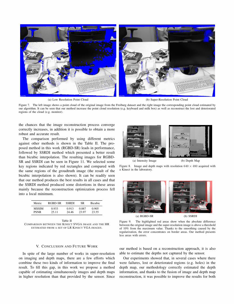
(a) RGBD-SR (b) SSRDI

Figure 9. The highlighted red areas show when the absolute differencebetween the original image and the super-resolution image is above a thresholdof 10% from the maximum value. Thanks to the smoothing caused by theregularization, the error concentrates on border areas. Our method presentsless areas with errors.

our method is based on a reconstruction approach, it is also

able to estimate the depths not captured by the sensor.

Our experiments showed that, in several cases where there

were failures, lost or deteriorated regions (e.g. holes) in the

depth map, our methodology correctly estimated the depth

information, and thanks to the fusion of image and depth map

reconstruction, it was possible to improve the results for both

(a) Intensity image with RGBD-SR (b) Intensity image with SSRDI

(c) RGBD-SR (d) SSRDI (e) Bicubic (f) RGBD-SR (g) SSRDI (h) Bicubic

(i) RGBD-SR (j) SSRDI (k) Bicubic (l) RGBD-SR (m) SSRDI (n) Bicubic

Figure 11. Images produced with the our method (RGBD-SR) and the SSRDI method. We can see that both methods produce better visual appearance whencompared to the bicubic interpolation. However, the SSRDI method falls into local minimum in some areas as shown in Figures 11g and 11m .

(a) Depth with RGBD-SR (b) Depth with SSRDI

Figure 10. Depth maps produced by the our methodology (RGBD-SR) andthe SSRDI method.

images and the depth maps.

As future work we intend to adapt the reconstruction model

to different luminance conditions and extend it to handle color

information as discussed in [17].

REFERENCES

[1] M. Meilland and A. I. Comport, “Super-resolution 3D tracking andmapping,” Proc. ICRA, pp. 5717–5723, May 2013.

[2] J. Diebel and S. Thrun, “An application of markov random fields torange sensing,” in Advances in neural information processing systems,2005, pp. 291–298.

[3] Q. Yang, R. Yang, J. Davis, and D. Nister, “Spatial-depth super resolu-tion for range images,” in Proc. CVPR. IEEE, 2007, pp. 1–8.

[4] U. Mudenagudi, A. Gupta, L. Goel, A. Kushal, P. Kalra, and S. Banerjee,“Super resolution of images of 3d scenecs,” pp. 85–95, 2007.

[5] T. Tung, S. Nobuhara, and T. Matsuyama, “Simultaneous super-resolution and 3d video using graph-cuts,” in Proc. CVPR. IEEE,2008, pp. 1–8.

[6] B. Goldlucke and D. Cremers, “A superresolution framework for high-accuracy multiview reconstruction,” in Pattern Recognition. Springer,2009, pp. 342–351.

[7] A. V. Bhavsar and A. Rajagopalan, “Resolution enhancement in multi-image stereo,” IEEE Trans. PAMI, vol. 32, no. 9, pp. 1721–1728, 2010.

[8] M. Unger, T. Pock, M. Werlberger, and H. Bischof, “A convex approachfor variational super-resolution,” in Pattern Recognition, 2010, pp. 313–322.

[9] H. S. Lee and K. M. Lee, “Simultaneous Super-Resolution of Depth andImages Using a Single Camera,” Proc. CVPR, pp. 281–288, Jun. 2013.

[10] P. J. Huber, “Wiley series in probability and mathematics statistics,”Robust Statistics, pp. 309–312, 1981.

[11] J. Stuhmer, S. Gumhold, and D. Cremers, “Real-time dense geometryfrom a handheld camera,” in Pattern Recognition, 2010, pp. 11–20.

[12] A. Chambolle and T. Pock, “A first-order primal-dual algorithm forconvex problems with applications to imaging,” Journal of Mathematical

Imaging and Vision, vol. 40, no. 1, pp. 120–145, 2011.

[13] T. Pock and A. Chambolle, “Diagonal preconditioning for first orderprimal-dual algorithms in convex optimization,” in Proc. ICCV. IEEE,2011, pp. 1762–1769.

[14] D. Scharstein and R. Szeliski, “A taxonomy and evaluation of densetwo-frame stereo correspondence algorithms,” International journal of

computer vision, vol. 47, no. 1-3, pp. 7–42, 2002.

[15] J. Sturm, N. Engelhard, F. Endres, W. Burgard, and D. Cremers, “ABenchmark for the Evaluation of RGB-D SLAM Systems,” in Proc.

IROS, Oct. 2012.

[16] F. Steinbrucker, J. Sturm, and D. Cremers, “Real-time visual odometryfrom dense rgb-d images,” in Proc. ICCV. IEEE, 2011, pp. 719–722.

[17] B. Goldluecke, E. Strekalovskiy, and D. Cremers, “The natural vectorialtotal variation which arises from geometric measure theory,” SIAM

Journal on Imaging Sciences, vol. 5, no. 2, pp. 537–563, 2012.