Simulations and Experiments on Low-Pressure Permeation of

Simulations and Experiments onLow-Pressure Permeation of Fabrics:Part II—The Variable Gap Model and

Prediction of Permeability

M. T. SENOGUZ, F. D. DUNGAN, A. M. SASTRY1 AND J. T. KLAMO

Department of Mechanical Engineering2140 G.G. Brown Building

2350 Hayward StreetThe University of MichiganAnn Arbor, MI 48109-2125

ABSTRACT: Use of the creeping flow assumption provides a computationally efficientand accurate means of predicting flow fronts in reinforcement media in many technologi-cally important polymer processes. In the case of fabrics, this creeping flow is shown to pro-ceed primarily through the gaps in fabrics, with capillarity playing little if any role forcommonly used materials. This finding has important implications for selection of strategyin modeling manufacturing processes of such materials. Namely, in the presence of fabricdeformation which induces local shear, changes in the gap architecture greatly affect theflow patterns, and are not well predicted by tensor transformation of Darcy-type permeabili-ties. A simple, classic flow model is adapted to the case of fabrics penetrated by low-pressureviscous liquids after careful analysis of fabric architecture. An applicability range of thiscreeping flow model, the variable gap model, is developed. The present paper gives themodel assumptions, and confirmation of its agreement with more sophisticated calculations.A demonstration of the approach for an unbalanced fabric (Knytex 24 5×4 unbalancedplain-woven glass fabric) shows excellent prediction of the bounds on flow behavior, andsupports our earlier experimental findings on flow front orientation. This approach alsoshows clear superiority to semi-empirical, geometry-based models, since no fitting parame-ters at all are used in the modeling: only the constituent materials’ geometry and propertiesare needed. This methodology is better able to predict trends in flow fronts, both qualita-tively and quantitatively, than semi-empirical fitting. Extension of this work to realistic pro-duction processes is planned.

1Author to whom correspondence should be addressed. E-mail: [email protected]

1285Journal of COMPOSITE MATERIALS, Vol. 35, No. 14/2001

0021-9983/01/14 1285–38 $10.00/0 DOI: 10.1106/HWL5-599F-8NA8-XAN0© 2001 Technomic Publishing Co., Inc.

Journal Online at http://techpub.metapress.com

INTRODUCTION

LOW-PRESSURE PENETRATION OF fabrics by viscous fluid is a key phenomenonin many technologically important composite processes. The majority of parts

involved presents some degree of curvature. Thus, development of a robust de-scription of fabrics is crucial for fabrics undergoing deformation (primarily shear).In the first part of this work (Dungan et al., 2001), a 3D model for an unbalancedplain-woven fabric was developed. This was motivated by the failure of simple ge-ometry models or empirical models to predict permeability of such fabrics in shear.In this part of the work, we use the newly developed fabric model to predict perme-ability of fabric in both sheared and unsheared configurations, using an approxima-tion for flow channel shape in the fabric. This model, unlike previous approachesused in predicting fabric permeability in either sheared or unsheared configura-tions, employs no fitting parameters.

Flow through reinforcements and between layers is hypothesized here to pre-sent a complex flow path which requires more detailed modeling than the com-mon empirical or geometric modifications to Darcy’s law, including theCarman-Kozeny equation, which typically involve calculation of permeabilitiesof the woven fabrics using fiber radius, overall volume fraction, and some empiri-cally-determined constants. In the regions where the volume fraction is high, theincreased fiber surface area with respect to the gap area creates a high viscousshear force, which reduces apparent permeability. Conversely, high ratios of sur-face area to gap area enhance capillary flow. This additional driving force, actingon the surface of the fluid, increases the permeability of the media, motivatingour study of the effect of capillary pressure as a momentum source. Use of a linearflow theory allows development of an equivalent expression for these permeabili-ties.

Experimentation on three scales was performed in the present study to assessthe relative importance of these phenomena: (1) single fiber contact angle mea-surements; (2) tow-level capillary pressure experiments; and (3) radial fab-ric-level permeability experiments. Each of these gave insight into the flow dy-namics at the microscale, and motivated some significant aspect of the numericalstudy. The single fiber experiments allowed calculation of the static contact angle,and thus a calculation of capillary pressure in a tow. The tow impregnation experi-ments allowed determination of intratow permeability, using the capillary pres-sure determined via contact angles. The radial permeability experiments withsheared and unsheared fabrics gave us insight into the effects of changing geome-try on the overall fabric permeability.

Simulations were performed on two scales. First, a full Navier-Stokes simula-tion for flow in a gap/tow region was performed. Second, a simplified flow calcu-lation based directly on information from the fabric model was developed to calcu-late permeabilities by considering only flow in the gap regions. Finally, we

1286 M. T. SENOGUZ, F. D. DUNGAN, A. M. SASTRY AND J. T. KLAMO

compare our linear model based on fabric architecture to experimental permeabil-ity data, and discuss the range of applicability and possible improvements to themodel.

ANALYSIS OF KEY EFFECTS IN RTM PROCESSES

Overview of Previous Work

Some simplification in the modeling of resin flow through the interstices andbetween layers of fiber beds is necessitated by the present impracticality of numer-ically solving the full Navier-Stokes equations in a stochastically- or near-regu-larly-arranged array of inclusions in the path of the flow front (e.g., Sastry, 2000).Percolation (i.e., low Reynolds number, Newtonian flows in macroscopically ho-mogeneous domains) was described originally by Darcy (1856), who developedthe constitutive description by observing water flow through beds of sand. Appli-cation of Darcy’s model to composite processes, from laminates to molded materi-als, is widespread. The percolation flow is generally applied to thermosetting res-ins in autoclave (laminate) or liquid molding processes. The familiar Darcy modelmay be written

(1)

where v is the average fluid velocity, µ is the fluid viscosity, K is the permeabilityof the porous medium, and ∇P is the pressure gradient and can be written intensorial form for anisotropic preforms, where up to 3 scalar permeabilities are re-quired in the plane case. Such implementations thus require determination of thepermeability or components of a permeability tensor, via experimental or theoreti-cal means. In application to actual processing, various factors are commonly usedto account for flow “tortuosity,” or circuitousness of the path that must be tra-versed to penetrate the material, the shape of the particles, material anisotropy, andthe average volume fraction. Several modifications to Equation (1) have thus beenproposed in the polymer processing arena and in other areas of fluid-structure in-teraction; for example, Kozeny (1927) treated a permeated porous medium as abundle of capillary tubes and obtained a relationship to adapt Darcy’s law to in-clude capillarity effects with an empirical relation; Blake (1922) derived a similarexpression. Carman (1937) modified Kozeny’s work by defining S, the specificsurface with respect to a unit volume of solid, instead of a unit volume of porousmedium. The “Kozeny-Carman relationship” arose through these sequential con-tributions. Carman (1937) experimentally determined a range of “Kozeny con-stants” for a variety of packing schemes and geometries of reinforcements. Thisconstant is determined empirically from

Low-Pressure Permeation of Fabrics: Part II 1287

−= ∇

µK

v P

(2)

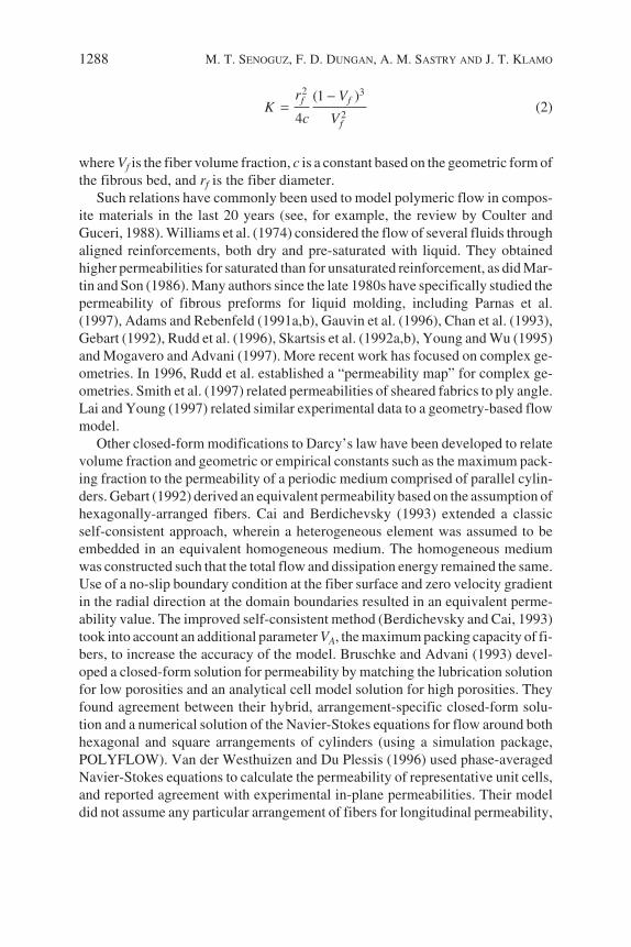
where Vf is the fiber volume fraction, c is a constant based on the geometric form ofthe fibrous bed, and rf is the fiber diameter.

Such relations have commonly been used to model polymeric flow in compos-ite materials in the last 20 years (see, for example, the review by Coulter andGuceri, 1988). Williams et al. (1974) considered the flow of several fluids throughaligned reinforcements, both dry and pre-saturated with liquid. They obtainedhigher permeabilities for saturated than for unsaturated reinforcement, as did Mar-tin and Son (1986). Many authors since the late 1980s have specifically studied thepermeability of fibrous preforms for liquid molding, including Parnas et al.(1997), Adams and Rebenfeld (1991a,b), Gauvin et al. (1996), Chan et al. (1993),Gebart (1992), Rudd et al. (1996), Skartsis et al. (1992a,b), Young and Wu (1995)and Mogavero and Advani (1997). More recent work has focused on complex ge-ometries. In 1996, Rudd et al. established a “permeability map” for complex ge-ometries. Smith et al. (1997) related permeabilities of sheared fabrics to ply angle.Lai and Young (1997) related similar experimental data to a geometry-based flowmodel.

Other closed-form modifications to Darcy’s law have been developed to relatevolume fraction and geometric or empirical constants such as the maximum pack-ing fraction to the permeability of a periodic medium comprised of parallel cylin-ders. Gebart (1992) derived an equivalent permeability based on the assumption ofhexagonally-arranged fibers. Cai and Berdichevsky (1993) extended a classicself-consistent approach, wherein a heterogeneous element was assumed to beembedded in an equivalent homogeneous medium. The homogeneous mediumwas constructed such that the total flow and dissipation energy remained the same.Use of a no-slip boundary condition at the fiber surface and zero velocity gradientin the radial direction at the domain boundaries resulted in an equivalent perme-ability value. The improved self-consistent method (Berdichevsky and Cai, 1993)took into account an additional parameter VA, the maximum packing capacity of fi-bers, to increase the accuracy of the model. Bruschke and Advani (1993) devel-oped a closed-form solution for permeability by matching the lubrication solutionfor low porosities and an analytical cell model solution for high porosities. Theyfound agreement between their hybrid, arrangement-specific closed-form solu-tion and a numerical solution of the Navier-Stokes equations for flow around bothhexagonal and square arrangements of cylinders (using a simulation package,POLYFLOW). Van der Westhuizen and Du Plessis (1996) used phase-averagedNavier-Stokes equations to calculate the permeability of representative unit cells,and reported agreement with experimental in-plane permeabilities. Their modeldid not assume any particular arrangement of fibers for longitudinal permeability,


−=

2 3

2

(1 )

4f f

f

r VK

c V

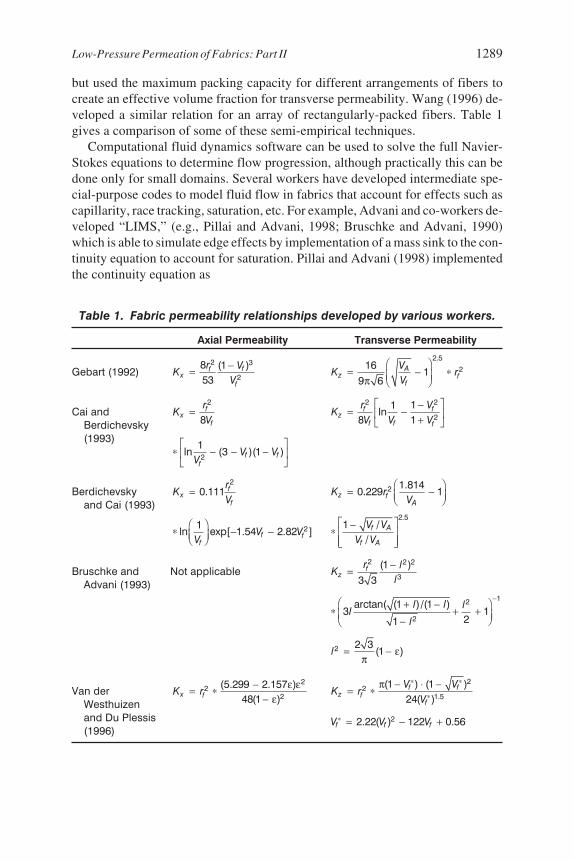
but used the maximum packing capacity for different arrangements of fibers tocreate an effective volume fraction for transverse permeability. Wang (1996) de-veloped a similar relation for an array of rectangularly-packed fibers. Table 1gives a comparison of some of these semi-empirical techniques.

Computational fluid dynamics software can be used to solve the full Navier-Stokes equations to determine flow progression, although practically this can bedone only for small domains. Several workers have developed intermediate spe-cial-purpose codes to model fluid flow in fabrics that account for effects such ascapillarity, race tracking, saturation, etc. For example, Advani and co-workers de-veloped “LIMS,” (e.g., Pillai and Advani, 1998; Bruschke and Advani, 1990)which is able to simulate edge effects by implementation of a mass sink to the con-tinuity equation to account for saturation. Pillai and Advani (1998) implementedthe continuity equation as


Table 1. Fabric permeability relationships developed by various workers.

Axial Permeability Transverse Permeability

Gebart (1992)

Cai andBerdichevsky(1993)

Berdichevskyand Cai (1993)

Bruschke andAdvani (1993)

Not applicable

Van derWesthuizenand Du Plessis(1996)

2 3

2

8 (1 )53

ffx

f

r VK

V-=

π

2.5

2161

9 6A

z ff

VK r

V

Ê ˆ= - *Á ˜Ë ¯

2

8f

xf

rK

V=

2 2

2

11ln

8 1f f

zf f f

r VK

V V VÈ ˘-

= -Í ˙+Î ˚

21

ln (3 )(1 )f ff

V VV

È ˘* - - -Í ˙

Î ˚

20.111 f

xf

rK

V= 2 1.814

0.229 1z fA

K rV

Ê ˆ= -Á ˜Ë ¯

2 2 2

3(1 )

3 3f

zr l

Kl

-=

12

2

arctan( (1 )/(1 )3 1

21

l l ll

l

-Ê ˆ+ -* + +Á ˜̄Ë -

επ

2 2 3(1 )l = -

ε εε

22

2(5.299 2.157 )

48(1 )x fK r-= *

-π 2

21.5

(1 ) (1 )24( )f f

z ff

V VK r

V

* *

*- ◊ -

= *

21ln exp[ 1.54 2.82 ]f f

fV V

VÊ ˆ* - -Á ˜Ë ¯

2.51 /

/f A

f A

V VV V

È ˘-* Í ˙

Í ˙Î ˚

22.22( ) 122 0.56f f fV V V* = - +

(3)

where rfA is the micro-front radius in the sink and r1A and r2A are the tow and cell ra-dii, respectively. The right hand side of the equation, denoted SA, is the strength ofa type A sink, calculated as

(4)

where Kit is the tow permeability. “Front Tracking” is capable of simulating theformation of voids (Song et al., 1997) and “SIMTEC” (Lin et al., 1998) accountsfor capillary action. “SUPERTM” is another interactive filling simulation (Ismailand Springer, 1997). Chang and Hourng (1998) developed a two-dimensionalmodel for tow impregnation, taking into account micro/macroscopic flow andvoid formation. Ambrosi and Preziosi (1998) developed a model for flow dynam-ics in an elastically deforming environment.

Flow in tows versus gaps or voids has been specifically studied by a number ofworkers. Shih and Lee (1998), for example, used six different types of glass fiberreinforcements to determine the effect of fiber architecture on apparent permeabil-ity. The reinforcements included 4-harness woven, plain weave, random fiber andstitched fiber mats. They argued that the gap size between the tows and the connec-tivity of the gaps control permeability. Kolodziej et al. (1998) proposed a theoreti-cal model which accounted specifically for gaps as caverns or fissures inside thebundle of fibers. Both diameter of fibers and also diameter of gaps inside the fiberbundles were incorporated in the model. They reported that tow heterogeneity candecrease or increase tow permeability, depending on the critical dimensionless ra-dius of these gaps. Heterogeneity was identified as the probable cause of deviationof permeabilities from permeability models, which assume uniformity inside thefiber bundles.

Capillarity has been advanced by a number of workers as an explanation for en-hanced flow in fabrics. Analytical and numerical estimates of its relative impor-tance have been made by a number of workers. Lekakou and Bader (1998), for ex-ample, modeled macro- and micro-flow, including capillary pressure. Theyperformed numerical parametric studies to correlate the effects of inter-tow andintra-tow volume fractions, different pressures, and fiber diameters on apparentpermeabilities. Hourng and Chang (1998) investigated edge flow and the effect ofcapillary pressure on edge flow. They suggested that for edges larger than the criti-


⋅= −

εµ

�

1ln

itfA

AfA

fA

K Pr

rr

r

− ε ∇ ⋅ ⋅ ∇ = µ −

�

2 212

1

2 ( )

1

fA fA

AA

A

r rKP

rr

r

cal value of 2K0.5, where K is the permeability, the edge effect cannot be ne-glected. Using numerical simulations, Chang et al. (1998) stated that the capillaryeffect is limited to capillary numbers less than O(10–2). The capillary number,given by

(5)

is the ratio of viscous forces to surface forces. A small capillary number repre-sents strong capillary action. Hourng and Chang (1998) proposed thatcapillarity be neglected for conventional RTM processes which usuallyhave higher injection pressures than 10 kPa. Ahn et al. (1991) experimentally ob-served that pressure dependence in capillarity begins around Ca ~ O(10–6). Inhis numerical study, Young (1996) reported that below a critical capillary num-ber, the fluid in the tows moves faster than the fluid between the tows becauseof the additional capillary pressure. Conversely, above the critical capillary num-ber, the flow between the tows dominates. The critical number was found to be 1 ×10–4 though he cautioned that this number might change for different preformtypes.

Determination of capillary pressure is generally made using the solid/liquid(droplet) contact angle. Dynamic effects cause the contact angle to deviatefrom the static capillary pressure. It is generally difficult to measure the dy-namic angle, but Skartsis et al. (1992c) proposed that for capillary number up toO(10–4), the static contact angle provided an excellent approximation to the dy-namic contact angle. Thus, for Re < 3000, such as creeping flow in porous me-dium, he suggested use of static contact angle rather than dynamic contact angle.These relationships and assumptions have been tested experimentally. For exam-ple, Ahn et al. (1991) measured permeability and capillary pressures simulta-neously by controlling both positive pressure at the inlet and pressure against theflow in the mold. By finding the negative piston pressure preventing flow frontpenetration in the fabric, the capillary pressure for that fabric was found. They re-ported capillary pressures as high as 37 kPa for T-300 carbon fibers, conclud-ing that although capillary pressure is negligible for an injection process, it maybe important for low pressure processes such as prepregging. They also ob-served that the Carman-Kozeny estimation of permeability deviated from the ex-perimental results for high porosity fabrics, while the Young-Laplace equation[see Equation (6) below] gave consistent results with experiments for capillarypressure.

Previous studies on RTM with fabrics have thus emphasized various manufac-turing factors, but most have implemented flow models in which pressure gradientand velocity are related linearly, with corrections for surface and geometry effects.We now examine the underlying contribution of surface effects, specifically


µ −=

σv

Ca

capillarity, by analytical means. First, we develop equivalence relationships forvarious creeping flows, in order to compare the gap and intra-tow permeabilitiesfor a fabric. We then compare these calculations with experiments in the fabricsystem considered in this two-part work, i.e., Knytex 24 5×4 unbalancedplain-woven glass fabric.

Comparison of Creeping Flows and Model Development

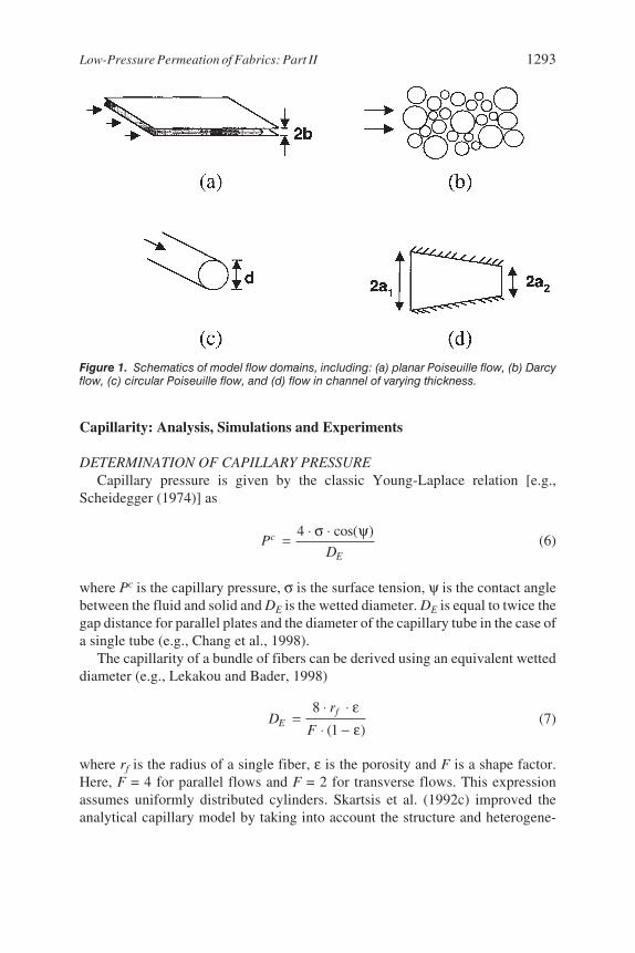
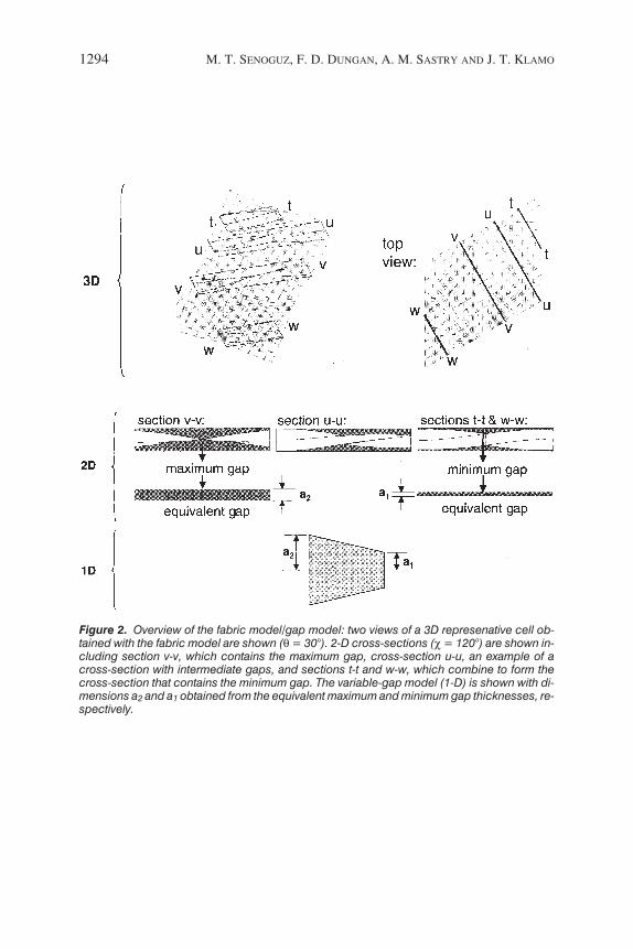
The proportionality of velocity and pressure gradient is central to modelingclassic creeping flows wherein the scaling parameter, “permeability,” may bederived as in Table 2. Schematics of each case are given as Figure 1. “PlanePoiseuille flow” describes steady-state flow between two infinitely long parallelplates separated by a distance 2b (e.g., Kundu, 1990). Circular Poiseuille flow re-fers to steady flow in a tube of diameter d. Flow in a channel of linearly varyingthickness describes flow in a channel with inlet half-thickness a1, outlethalf-thickness a2, and channel length L (e.g., Batchelor, 1967). We hereafter referto the model just described [Figure 1(d) and last line of Table 2] as the VGM, orVariable Gap Model. In the sections that follow, we describe a technique for re-ducing information from a 3D fabric model (developed in Part I of this work,Dungan et al., 2001) to 2D sections, to a 1D model, i.e., the VGM. Figure 2 gives a“roadmap” of the steps which proceeded from the numerical and experimentalstudies described presently. In order to eliminate capillarity as a factor in the anal-ysis, i.e. to show that inter- rather than intra-tow flow was the dominant factor, wefirst performed an analysis of capillary pressure in the material studied, Knytex 245×4.


Table 2. Equivalent permeabilities for various creeping flows.

Velocity EquationPermeability

Constant

Darcy’s law K

Plane Poiseuille flow b2/3

Circular Poiseuille flow d2/32

Variable gap model

µK dP

vdx

-= ◊

µ

2( / 3)ave

b dPv

dx= - ◊

µ

2( / 32)ave

d dPv

dx= - ◊

µ

2 21 2

21 2

43 ( )

ave

a aa a dP

vdx

Ê ˆ-Á ˜+Ë ¯

= ◊2 21 2

2 21 2

43 ( )

a aa a+

Capillarity: Analysis, Simulations and Experiments

DETERMINATION OF CAPILLARY PRESSURECapillary pressure is given by the classic Young-Laplace relation [e.g.,

Scheidegger (1974)] as

(6)

where Pc is the capillary pressure, σ is the surface tension, ψ is the contact anglebetween the fluid and solid and DE is the wetted diameter. DE is equal to twice thegap distance for parallel plates and the diameter of the capillary tube in the case ofa single tube (e.g., Chang et al., 1998).

The capillarity of a bundle of fibers can be derived using an equivalent wetteddiameter (e.g., Lekakou and Bader, 1998)

(7)

where rf is the radius of a single fiber, ε is the porosity and F is a shape factor.Here, F = 4 for parallel flows and F = 2 for transverse flows. This expressionassumes uniformly distributed cylinders. Skartsis et al. (1992c) improved theanalytical capillary model by taking into account the structure and heterogene-


⋅ σ ⋅ ψ=

4 cos( )c

E

PD

⋅ ⋅ ε=

⋅ − ε8

(1 )f

E

rD

F

Figure 1. Schematics of model flow domains, including: (a) planar Poiseuille flow, (b) Darcyflow, (c) circular Poiseuille flow, and (d) flow in channel of varying thickness.


Figure 2. Overview of the fabric model/gap model: two views of a 3D represenative cell ob-tained with the fabric model are shown (θ = 30°). 2-D cross-sections (χ = 120°) are shown in-cluding section v-v, which contains the maximum gap, cross-section u-u, an example of across-section with intermediate gaps, and sections t-t and w-w, which combine to form thecross-section that contains the minimum gap. The variable-gap model (1-D) is shown with di-mensions a2 and a1 obtained from the equivalent maximum and minimum gap thicknesses, re-spectively.

ity of the media, and reported agreement between analytical results and experi-ments.

CONTACT ANGLE MEASUREMENTSThe contact angle of corn oil (the fluid used in the fabric level experiments)

with the surface of a glass fiber (17.2 µm diameter) was measured under an opticallight microscope at room temperature. For fabric permeability experiments, bothclear (unsaturated) and dyed (saturated) oils were used. Both clear and dyed oil/fi-ber contact angles were thus measured. Material properties on the fibers, tows,fabric and oil are given in Table 3.

A numerical method developed by Wagner (1990) was used to calculate thecontact angle based upon the reduced droplet radius, reduced droplet length and fi-ber radius. This methodology was validated recently by Song et al. (1998) whoshowed that refinements in the contact angle measurement produced changes onthe order of 10–1 degrees. A mean value of 20.11 degrees with standard deviationof 3.39 was found for the contact angle for clear oil; the dyed oil had a mean con-tact angle of 12.96 degrees with a standard deviation of 5.67.


Table 3. Material properties for Knytex 24-5×4 and corn oil,both clear and dyed.

Knytex 24-5×4 Plain-Weave Fabric

Fiber composition E-glassDensity of fiber material 2590 kg/m3 (0.0935 lb/in3)Linear density of tows 207 yd/lbVolume fraction of one layer of fabric 45.4%Warp intratow volume fraction 78.6%Weft intratow volume fraction 78.2%Numbers of warp tows per inch 5Numbers of weft tows per inch 4Width of warp tows 5 mmWidth of weft tows 5 mmThickness of one layer of fabric 0.7366 mmNumber of glass fibrils per warp tow 4020Number of glass fibrils per weft tow 4020Diameter of a fibril 17.2 µmFabric lock angle 33 degrees

Clear Corn Oil

Density 893 kg/m3

Viscosity 0.040 kg/(m·s)

Dyed Corn Oil

Density 892 kg/m3

Viscosity 0.044 kg/(m·s)

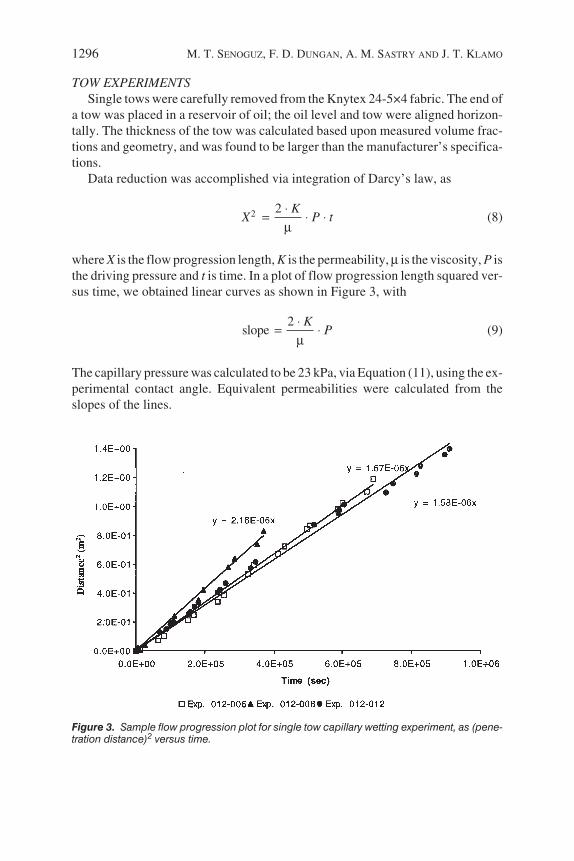
TOW EXPERIMENTSSingle tows were carefully removed from the Knytex 24-5×4 fabric. The end of

a tow was placed in a reservoir of oil; the oil level and tow were aligned horizon-tally. The thickness of the tow was calculated based upon measured volume frac-tions and geometry, and was found to be larger than the manufacturer’s specifica-tions.

Data reduction was accomplished via integration of Darcy’s law, as

(8)

where X is the flow progression length, K is the permeability,µ is the viscosity, P isthe driving pressure and t is time. In a plot of flow progression length squared ver-sus time, we obtained linear curves as shown in Figure 3, with

(9)

The capillary pressure was calculated to be 23 kPa, via Equation (11), using the ex-perimental contact angle. Equivalent permeabilities were calculated from theslopes of the lines.


⋅= ⋅ ⋅

µ2 2 K

X P t

⋅= ⋅

µ2

slopeK

P

Figure 3. Sample flow progression plot for single tow capillary wetting experiment, as (pene-tration distance)2 versus time.

The predicted permeabilities with different models and averaged experimentalresults are shown in Table 4. All predictions except Carman-Kozeny were an orderof magnitude off from experimental findings.

COMPARISON WITH SIMULATIONSSimulations were performed on prismatic sections, using the commercial CFD

software FLUENT (Fluent Inc., v. 5.0, 1999). A momentum source representingthe capillary pressure was added to the surface of the flow front. A Fortran algo-rithm tracing the flow front and adding a momentum source to necessary computa-tional cells was incorporated into the software via a user-defined material subrou-tine. The fluid mechanics are summarized as follows. The momentumconservation equation in FLUENT takes the form

(10)

where Fi is the volume-averaged drag force, given by

(11)

Elements designated as porous cells (having capillarity) were checked to deter-mine the volume fraction of oil in the cell and in the next cell in the flow direction.The flow front was located via addition of the momentum source to the conserva-tion equation at the flow boundaries (the calculated capillary pressure was multi-plied by the cross-sectional area of a single cell and the resulting surface force wasapplied to that cell in the flow direction as an equivalent body force). Comparisonof simulations showed this approach to be equivalent to addition of a body forcerepresenting increased flow momentum due to capillarity.

A rectangular flow domain was created with two different sections. The upperhalf was assigned a permeability of 1 × 10–12 m2 (suggested by experimental val-ues of permeability from the intratow wetting experiments); the lower portion was


∂τ∂ ∂ ∂ρ ⋅ + ρ ⋅ ⋅ = − + + ρ ⋅ +

∂ ∂ ∂ ∂( ) ( )

iji i j i i

j i j

Pv v v g F

t x x x

µ= − ⋅i i

i

F vK

Table 4. Predicted and experimental intratow permeabilities.

AxialPermeability

TransversePermeability

Carman-Kozeny 2.6 × 10–12 1.3 × 10–13

Gebart (1992) 1.95 × 10–13 2.93 × 10–14

Cai and Berdichevsky (1993) 1.01 × 10–13 5.91 × 10–14

Berdichevsky and Cai (1993) 1.41 × 10–13 3.51 × 10–14

Experiments 1.56 × 10–12 N/A

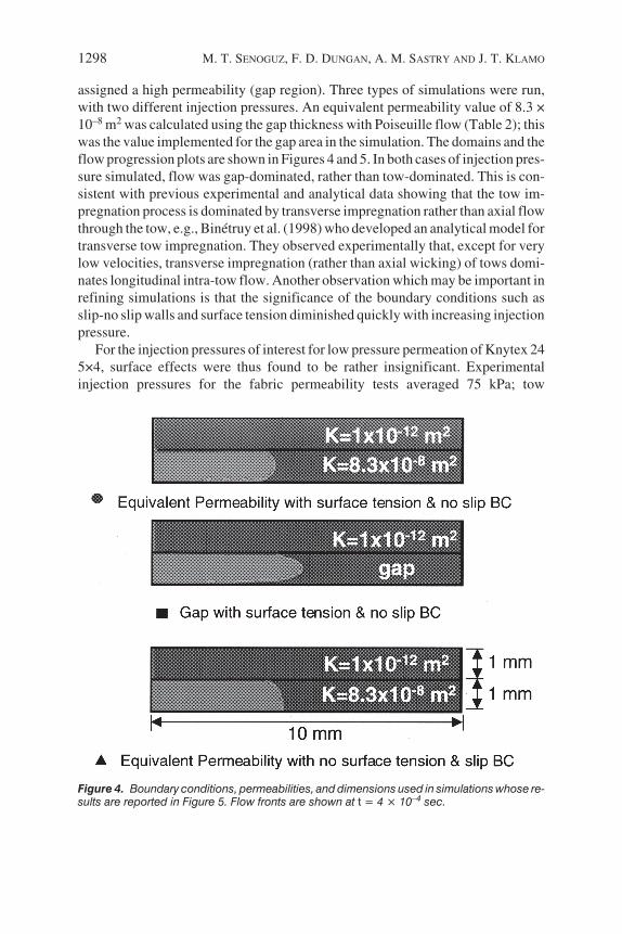
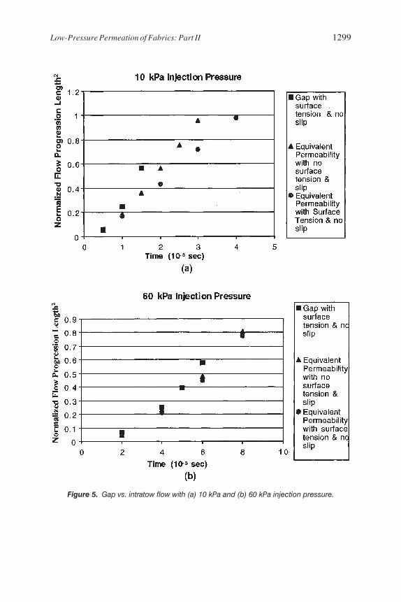
assigned a high permeability (gap region). Three types of simulations were run,with two different injection pressures. An equivalent permeability value of 8.3 ×10–8 m2 was calculated using the gap thickness with Poiseuille flow (Table 2); thiswas the value implemented for the gap area in the simulation. The domains and theflow progression plots are shown in Figures 4 and 5. In both cases of injection pres-sure simulated, flow was gap-dominated, rather than tow-dominated. This is con-sistent with previous experimental and analytical data showing that the tow im-pregnation process is dominated by transverse impregnation rather than axial flowthrough the tow, e.g., Binétruy et al. (1998) who developed an analytical model fortransverse tow impregnation. They observed experimentally that, except for verylow velocities, transverse impregnation (rather than axial wicking) of tows domi-nates longitudinal intra-tow flow. Another observation which may be important inrefining simulations is that the significance of the boundary conditions such asslip-no slip walls and surface tension diminished quickly with increasing injectionpressure.

For the injection pressures of interest for low pressure permeation of Knytex 245×4, surface effects were thus found to be rather insignificant. Experimentalinjection pressures for the fabric permeability tests averaged 75 kPa; tow


Figure 4. Boundary conditions, permeabilities, and dimensions used in simulations whose re-sults are reported in Figure 5. Flow fronts are shown at t = 4 × 10–4 sec.


Figure 5. Gap vs. intratow flow with (a) 10 kPa and (b) 60 kPa injection pressure.

experiments resulted in calculated capillary pressures of approximately 23 kPa forthe same material.

Tow Level Analyses: Application of the Variable Gap Model

Because of the dominance of gap flow for realistic processing cycles, a methodfor assessing the gap geometry using the fabric model was developed. As shownin Figure 2, the model accounted only for flow in the gaps of the fabric. Perthe VGM equation (Table 2), permeability is sensitive to narrow sections of aflow channel. Thus, using a Poiseuille approach with a single gap width wouldnot sufficiently capture the tortuosity of flow in a fabric. This is supported byevidence of the failure of simple volume fraction calculations to correctpermeabilities from the unsheared configuration to predict permeabilities insheared configurations. Though volume fraction certainly increases with shear,changes in the microarchitecture have a more significant effect, i.e., the placementof tows (barriers) is more significant than their volume fraction for this materialand shear range.

The fabric model developed as Part I of this work (Dungan et al., 2001) wasused to develop expressions for equivalent gap thickness for arbitrary sections.The gap between two layers of fabric was isolated directly from the fabric model,whereupon gap area was found. Two extreme cases were considered, suggested bythe characterizations of the effects of nesting in Part I—the cases of no nesting andmaximum nesting. Possible effects from deflections of the mold top were ruled outfor the experiment via finite element analysis (Dungan, 2000). The maximum de-flection at the center of the mold top was found to be 0.05% of the standard moldcavity thickness, so racetracking between the bottom of the mold top and the top ofthe fabric reinforcements was not considered.

In the case of no nesting, shown schematically as Figure 6(a), the gap areas be-tween the tows and a flat surface were measured for both the upper surface of thetows and their lower surface. The number of cross-sections taken for each shearangle (σ)-cross-section angle (χ) pair varied between 2 and 16. In most cases,cross-sections were taken at just 2 strategic locations: the cross-section passingthrough the middle of the symmetric cross-section, and the cross-section made upof two incomplete cross-sections of the same length, i.e., the cross-section whosetwo pieces were located in the middle of the range of incomplete cross-sections.Those locations were identified as representing minimum and maximum gaps, forany shear angle (θ)-cross-section angle (χ) pair.

In the case of no nesting, shown schematically as Figure 6(b), the gaps betweentwo fabric layers offset by Sa/2 in the warp direction and Sb/2 in the weft directionover an area of one representative cell were measured. For the maximum nestingcase, no trend was apparent from pictures of cross-sections or from initial mea-surements. The number of cross-sections taken for each shear angle (θ)-cross-sec-


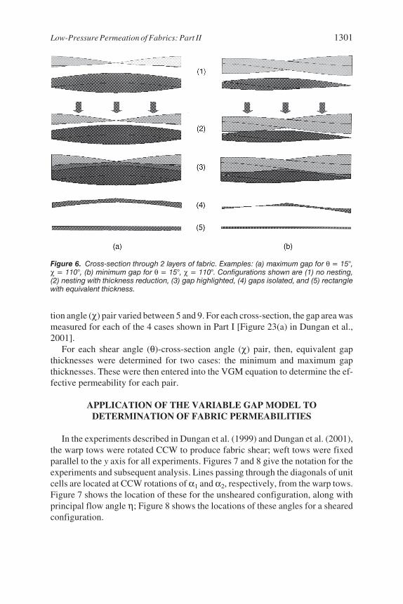
tion angle (χ) pair varied between 5 and 9. For each cross-section, the gap area wasmeasured for each of the 4 cases shown in Part I [Figure 23(a) in Dungan et al.,2001].

For each shear angle (θ)-cross-section angle (χ) pair, then, equivalent gapthicknesses were determined for two cases: the minimum and maximum gapthicknesses. These were then entered into the VGM equation to determine the ef-fective permeability for each pair.

APPLICATION OF THE VARIABLE GAP MODEL TODETERMINATION OF FABRIC PERMEABILITIES

In the experiments described in Dungan et al. (1999) and Dungan et al. (2001),the warp tows were rotated CCW to produce fabric shear; weft tows were fixedparallel to the y axis for all experiments. Figures 7 and 8 give the notation for theexperiments and subsequent analysis. Lines passing through the diagonals of unitcells are located at CCW rotations of α1 and α2, respectively, from the warp tows.Figure 7 shows the location of these for the unsheared configuration, along withprincipal flow angle η; Figure 8 shows the locations of these angles for a shearedconfiguration.


Figure 6. Cross-section through 2 layers of fabric. Examples: (a) maximum gap for θ = 15°,χ = 110°, (b) minimum gap for θ = 15°, χ = 110°. Configurations shown are (1) no nesting,(2) nesting with thickness reduction, (3) gap highlighted, (4) gaps isolated, and (5) rectanglewith equivalent thickness.


Figure 7. Angle notation for experimental data for an unsheared fabric case. The shaded arearepresents a typical experimental flow front shape.

Figure 8. Angle notation for experimental data for a sheared fabric case. The shaded area rep-resents a typical experimental flow front shape.

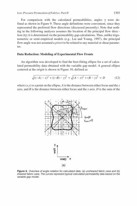
For comparison with the calculated permeabilities, angles γ were de-fined as shown in Figure 9. These angle definitions were convenient, since theyrepresented the preferred flow directions (discussed presently). Note that noth-ing in the following analyses assumes the location of the principal flow direc -tion (η); it is determined via the permeability gap calculations. Thus, unlike trigo-nometric or semi-empirical models (e.g., Lai and Young, 1997), the principalflow angle was not assumed a priori to be related to any material or shear parame-ter.

Data Reduction: Modeling of Experimental Flow Fronts

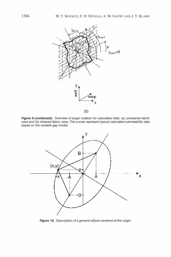
An algorithm was developed to find the best-fitting ellipse for a set of calcu-lated permeability data obtained with the variable gap model. A general ellipsecentered at the origin is shown in Figure 10, defined as

(12)

where (x,y) is a point on the ellipse, A is the distance between either focus and the yaxis, and B is the distance between either focus and the x axis. D is the sum of the


− − + − − + − + − =2 2 2 2(( ) ) (( ) ) ( ) ( )A x B y A x B y D

Figure 9. Overview of angle notation for calculated data: (a) unsheared fabric case and (b)sheared fabric case. The curves represent typical calculated permeability data based on thevariable gap model.


Figure 9 (continued). Overview of angle notation for calculated data: (a) unsheared fabriccase and (b) sheared fabric case. The curves represent typical calculated permeability databased on the variable gap model.

Figure 10. Description of a general ellipse centered at the origin.

distances between any point on the ellipse and the two foci. For any angle χ (mea-sured counterclockwise from the x axis),

(13)

and

(14)

Since tan(90°) tends to infinity,χ= 90° was treated as a special case with x = 0 and

(15)

A program was written to find the ellipse minimizing an error measure defined as

(16)

for a given set of N data points (Pi, Qi) and points (xi, yi) on the ellipse at corre-sponding angles χi. An additional constraint was introduced in order to ensure thatthe area of the ellipse was conserved. The area of the polygon defined by the datapoints (Pi, Qi) was calculated using

(17)

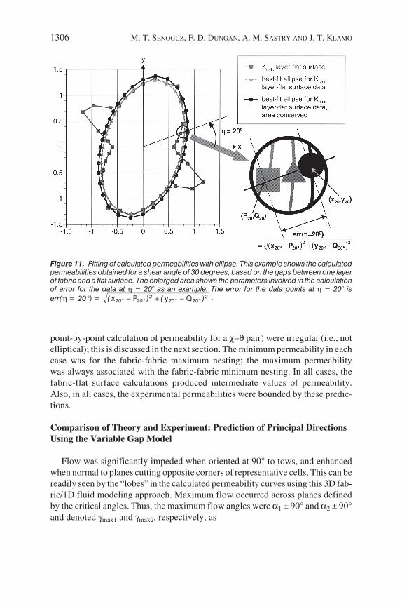
and the area of the best-fit ellipse was constrained to that area. A schematic of thiserror calculation for an actual case (χ = 20° and θ = 30°) is shown as Figure 11.

Comparison of Theory and Experiment: Prediction of Permeability Usingthe Variable Gap Model

Three cases were examined using the variable gap model to predict permeabil-ity: fabric-to-fabric with maximum nesting, fabric-to-fabric with minimum nest-ing, and fabric-to-flat surface. These three conditions represent the extremes of sit-uations occurring in a real mold, with the flat surface representing the mold top orbottom. The corresponding permeabilities, along with the experimental saturatedand unsaturated permeabilities, are shown in Figures 12, 13 and 14, for 0°, 15° and30° shear, respectively. In all cases, the calculated permeability curves (based on


= χtan( )y x

2 2 2 2

2 2 2 2 2 2

( 4 4 )

16 4 32 tan( ) 16 (tan( )) 4 (tan( ))

D A B Dy

A D AB B D

− − += ±− + − χ − χ + χ

− − += ±

− +

2 2 2 2

2 2

( 4 4 )

16 4

D A B Dy

B D

== − + −∑ 2 2

1

error ( ) ( )N

i i i ii

x P y Q

+ + +

=

χ − χ + + = + ∑

2 21 1 1

1

area 2 tan2 2 2

Ni i i i i i

i

x x y y

point-by-point calculation of permeability for a χ–θ pair) were irregular (i.e., notelliptical); this is discussed in the next section. The minimum permeability in eachcase was for the fabric-fabric maximum nesting; the maximum permeabilitywas always associated with the fabric-fabric minimum nesting. In all cases, thefabric-flat surface calculations produced intermediate values of permeability.Also, in all cases, the experimental permeabilities were bounded by these predic-tions.

Comparison of Theory and Experiment: Prediction of Principal DirectionsUsing the Variable Gap Model

Flow was significantly impeded when oriented at 90° to tows, and enhancedwhen normal to planes cutting opposite corners of representative cells. This can bereadily seen by the “lobes” in the calculated permeability curves using this 3D fab-ric/1D fluid modeling approach. Maximum flow occurred across planes definedby the critical angles. Thus, the maximum flow angles were α1 ± 90° and α2 ± 90°and denoted γmax1 and γmax2, respectively, as


Figure 11. Fitting of calculated permeabilities with ellipse. This example shows the calculatedpermeabilities obtained for a shear angle of 30 degrees, based on the gaps between one layerof fabric and a flat surface. The enlarged area shows the parameters involved in the calculationof error for the data at η = 20° as an example. The error for the data points at η = 20° iserr( = 20 ) = ( ) ( )20 20

220 20

2h ∞ - + -∞ ∞ ∞ ∞x P y Q .


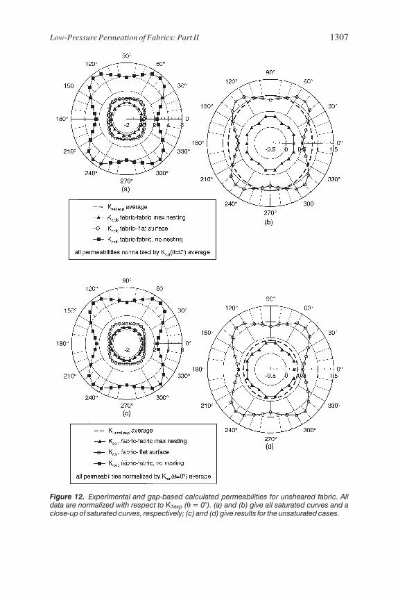
Figure 12. Experimental and gap-based calculated permeabilities for unsheared fabric. Alldata are normalized with respect to K1exp (θ = 0°). (a) and (b) give all saturated curves and aclose-up of saturated curves, respectively; (c) and (d) give results for the unsaturated cases.


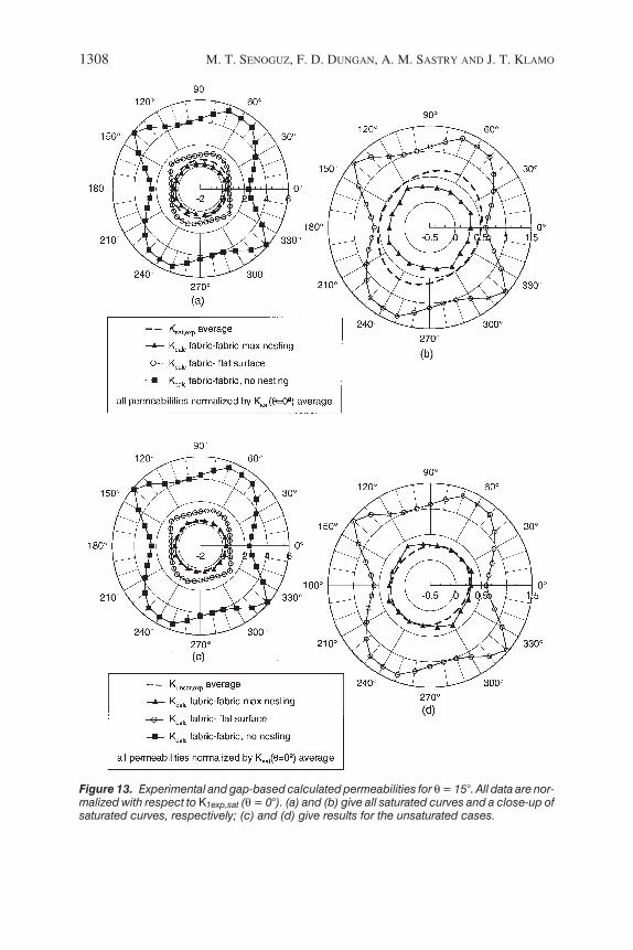
Figure 13. Experimental and gap-based calculated permeabilities for θ = 15°. All data are nor-malized with respect to K1exp,sat (θ = 0°). (a) and (b) give all saturated curves and a close-up ofsaturated curves, respectively; (c) and (d) give results for the unsaturated cases.


Figure 14. Experimental and gap-based calculated permeabilities for θ = 30°. All data are nor-malized with respect to K1exp,sat (θ = 0°). (a) and (b) give all saturated curves and a close-up ofsaturated curves, respectively; (c) and (d) give results for the unsaturated cases.

(18)

(19)

These are as shown in Figure 9. The minimum flow angles occurred across thewarp and weft directions, i.e., θ ± 90° and [0°,180°] (since the weft tows werefixed at 0°). These minimum angles γmin1 and γmin2, were defined as

(20)

(21)


γ = ° °min1 0 , 180

γ = θ ± °min2 90

γ = α ± °max2 1 90

γ = α ± °max1 2 90

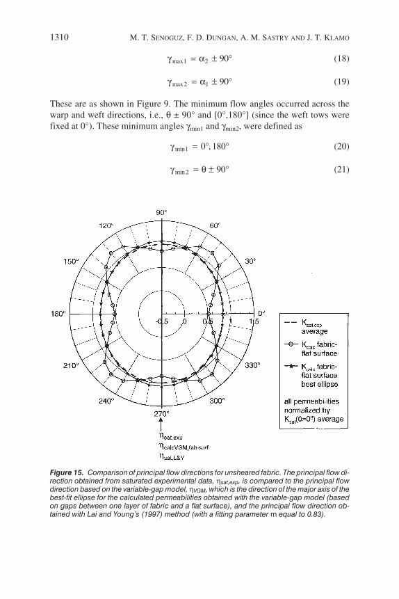
Figure 15. Comparison of principal flow directions for unsheared fabric. The principal flow di-rection obtained from saturated experimental data, ηsat,exp, is compared to the principal flowdirection based on the variable-gap model, ηVGM, which is the direction of the major axis of thebest-fit ellipse for the calculated permeabilities obtained with the variable-gap model (basedon gaps between one layer of fabric and a flat surface), and the principal flow direction ob-tained with Lai and Young’s (1997) method (with a fitting parameter m equal to 0.83).


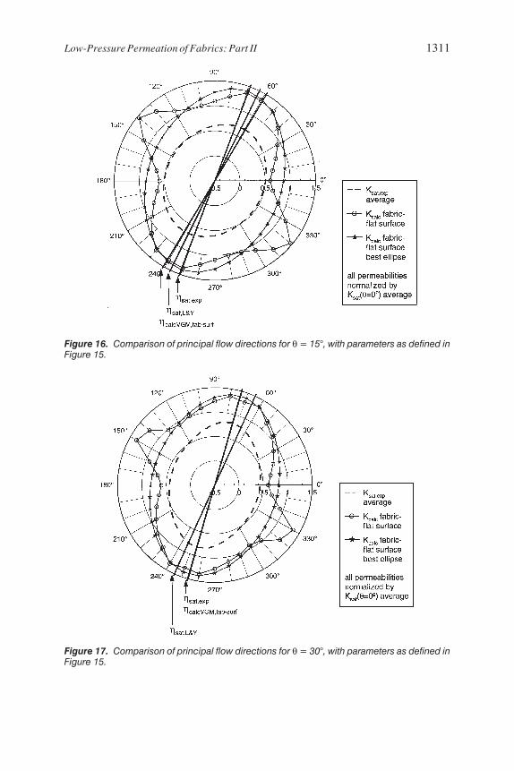
Figure 16. Comparison of principal flow directions for θ = 15°, with parameters as defined inFigure 15.

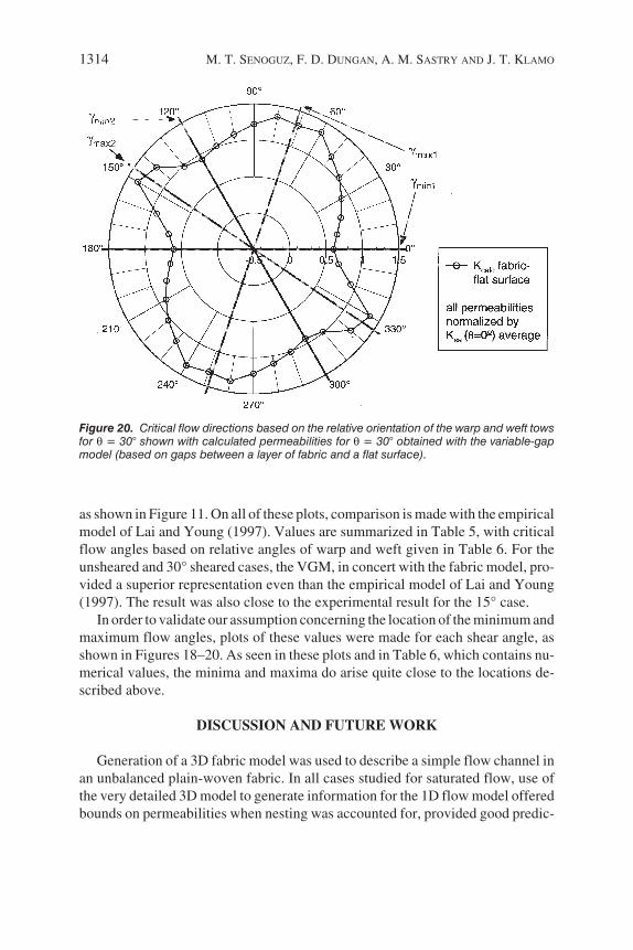
Figure 17. Comparison of principal flow directions for θ = 30°, with parameters as defined inFigure 15.

The “cloverleaf” patterns exhibited by the permeability data obtained with thevariable gap model as shown in Figures 12–14 result from these preferred direc-tions, which are artifacts of the 1D analysis performed for the fluids calculation.The flow favors the direction α2 ± 90° over α1 ± 90° for shear angles other thanzero because the plane across which the flow proceeds makes a larger angle withthe warp and the weft for the α2 ± 90° case than for the α1 ± 90° case. Flow in theminimum flow direction (0°) is the most restricted because it hits the weft tows“dead-on”; the remaining (warp) tows for the Knytex 24 5×4 have no gaps be-tween them (see Dungan et al., 2001, Figure 1), resulting in a low channel area forthe normal flow.

The predictions of principal flow angles (η) are shown in Figures 15–17, for 0°,15° and 30° shear, respectively. These principal angles were determined by loca-tion of the major axis of a best-fit ellipse through all calculated 1D permeabilities,


Table 5. Comparison of principal flow directions fromexperiments, calculations, and Lai and Young’s model.

Shear Angle(degrees) 15 30

ηexp,unsat (degrees) 47.4 74.2

ηexp,sat (degrees) 59.2 74.0

ηcalc (degrees)(% error relative to

ηexp,sat)

69.4(17.2)

73.8(0.270)

ηLai&Young,unsat,m=1.0

(degrees)(% error relative to

ηexp,unsat)

60.2(27.0)

63.6(14.3)

ηLai&Young,sat,m=0.83

(degrees)(% error relative to

ηexp,sat)

63.7(7.60)

65.4(11.6)

Note: All the principal flow angles are 90 degrees for unsheared fabric.

Table 6. Critical flow directions based on the relativeorientation of the warp and weft tows.

Shear Angle (degrees) 0 15 30

γmax1 (degrees) 51.8 61.3 71.6γmax2 (degrees) 128 137 146γmin1 (degrees) 0 0 0γmin2 (degrees) 90 105 120


Figure 18. Critical flow directions based on the relative orientation of the warp and weft towsfor unsheared fabric shown with calculated permeabilities for θ = 0° obtained with the vari-able-gap model (based on gaps between a layer of fabric and a flat surface).

Figure 19. Critical flow directions based on the relative orientation of the warp and weft towsfor θ = 15° shown with calculated permeabilities for θ = 15° obtained with the variable-gapmodel (based on gaps between a layer of fabric and a flat surface).

as shown in Figure 11. On all of these plots, comparison is made with the empiricalmodel of Lai and Young (1997). Values are summarized in Table 5, with criticalflow angles based on relative angles of warp and weft given in Table 6. For theunsheared and 30° sheared cases, the VGM, in concert with the fabric model, pro-vided a superior representation even than the empirical model of Lai and Young(1997). The result was also close to the experimental result for the 15° case.

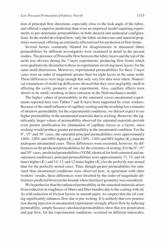
In order to validate our assumption concerning the location of the minimum andmaximum flow angles, plots of these values were made for each shear angle, asshown in Figures 18–20. As seen in these plots and in Table 6, which contains nu-merical values, the minima and maxima do arise quite close to the locations de-scribed above.

DISCUSSION AND FUTURE WORK

Generation of a 3D fabric model was used to describe a simple flow channel inan unbalanced plain-woven fabric. In all cases studied for saturated flow, use ofthe very detailed 3D model to generate information for the 1D flow model offeredbounds on permeabilities when nesting was accounted for, provided good predic-


Figure 20. Critical flow directions based on the relative orientation of the warp and weft towsfor θ = 30° shown with calculated permeabilities for θ = 30° obtained with the variable-gapmodel (based on gaps between a layer of fabric and a flat surface).

tion of principal flow directions, especially close to the lock angle of the fabric,and offered a superior prediction than even an empirical model requiring experi-ments to pre-determine permeabilities in both sheared and unsheared configura-tions. In the model developed here, only the fabric architecture and material prop-erties were used, offering an extremely efficient tool for prediction of flow fronts.

Several factors commonly blamed for disagreements in measured fabricpermeabilities by different investigators were examined in detail in the presentstudies. The presence of Poiseuille flow between the fabric layers and the top of themold was obvious during the 7-layer experiments, producing flow fronts whichwere qualitatively dissimilar to those in experiments involving more layers, for thesame mold dimensions. Moreover, experimental permeabilities for these 7-layercases were an order of magnitude greater than for eight layers in the same mold.These differences were large enough that only very few data were taken. Numeri-cal simulations of mold top deflections showed that they were negligibly small inaffecting the cavity geometry of our experiments. Also, capillary effects wereshown to be small, resulting in their omission in the fluid mechanics model.

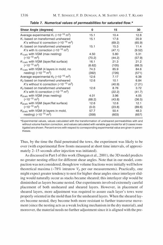
The higher values of permeability in the saturated versus unsaturated experi-ments reported here (see Tables 7 and 8) have been supported by some workers.Because of the small influence of capillary wetting and the resulting low estimatesof intratow permeability for the experimental conditions, we did not expect to seehigher permeability in the unsaturated materials due to wicking. However, the sig-nificantly larger values of permeability observed for saturated materials provideeven greater justification for elimination of capillary forces as a factor, sincewicking would produce greater permeability in the unsaturated condition. For the0°, 15° and 30° cases, the saturated principal permeabilities were approximately140%, 120% and 100% higher (K1) and 130%, 110% and 80% higher (K2) than theanalogous unsaturated cases. These differences were exceeded, however, by dif-ferences in the predicted permeabilities for the extremes of nesting. For the 0°, 15°and 30° cases, predicted permeabilities (VGM, identical for both saturated and un-saturated conditions), principal permeabilities were approximately 17, 15, and 16times higher (K1) and 14, 13, and 12 times higher (K2) for the perfectly non-nestedthan for the perfectly nested cases. Thus, though greater permeabilities for satu-rated than unsaturated conditions were observed here, in agreement with otherworkers’ results, these differences were dwarfed by the order-of-magnitude dif-ferences predicted between the bounds when interlayer geometry was considered.

We hypothesize that the enhanced permeability in the saturated materials arisesfrom reduction in roughness of fibers and fiber bundles due to the coating with oil.As with reduction of friction factors in smooth pipes, we suspect that the oil coat-ing significantly enhances flow due to pre-wetting. It is unlikely that tow penetra-tion during injection in unsaturated experiments strongly affects flow by reducingpermeability, simply because calculated permeabilities show that tow penetrationand gap flow, for the experimental conditions, occurred on different timescales.


Thus, by the time the fluid penetrated the tows, the experiment was likely to beover (with experimental flow fronts measured at short time intervals, of approxi-mately 2–15 seconds after injection was initiated).

As discussed in Part I of this work (Dungan et al., 2001), the 3D model predictsno greater nesting effect for different shear angles. Note that in our model, com-paction was not considered, though tow volume fractions were initially well belowtheoretical maxima (~78% intratow Vf, per our measurements). Practically, onemight expect greater tendency to nest for higher shear angles since interlayer slid-ing would naturally occur as stacks became sheared; this interlayer slip would bediminished as layers became nested. Our experiments involved extremely carefulplacement of both unsheared and sheared layers. However, in placement ofsheared layers, more adjustment was required to assure each layer’s tows wereproperly oriented in the mold than for the unsheared layers. When the sheared lay-ers become nested, they become both more resistant to further transverse move-ment (since the nesting acts as a weak locking mechanism in the dry material), andmoreover, the material needs no further adjustment since it is aligned with the pre-


Table 7. Numerical values of permeabilities for saturated flow.*


Average experimental K1 (∗10–10 m2) 15.1 10.4 12.6K1 based on transformed unsheared

K’s without Vf correction (∗10–10 m2)15.1 17.6

(69.2)20.9

(65.9)K1 based on transformed unsheared

K’s with Vf correction (∗10–10 m2)15.1 15.3

(47.1)11.4

(9.52)K1calc with VGM (max nesting)

(∗10–10 m2)4.50

(70.2)5.80

(44.2)5.31

(57.9)K1calc with VGM (layer/flat surface)

(∗10–10 m2)16.1

(6.62)21.3(105)

21.2(68.3)

K1calc with VGM (4 layers in mold, nonesting) (∗10–10 m2)

74.3(392)

85.9(726)

84.6(571)



(40.9)6.84



(22.2)3.72


(∗10–10 m2)4.01

(68.2)3.96

(43.8)4.05


(∗10–10 m2)12.6(0.0)

12.6(23.8)

12.1(89.6)

K2calc with VGM (4 layers in mold,nesting) (∗10–10 m2)

57.7(358)

50.4(603)

48.3(657)

*Experimental values, values calculated with the transformation of unsheared permeabilities with andwithout volume fraction correction, and values calculated with variable gap model for all 3 cases inves-tigated are shown. Percent errors with respect to corresponding experimental value are given in paren-theses.

vious (acceptably aligned) layer. In the initial experiments performed for thiswork (Dungan et al., 1999) and in the further experiments performed in Parts I andII of the present portions of the work, these types of adjustments were routinelyperformed. We suspect that preferential nesting in the sheared versus theunsheared experiments may have played a role.

In contrast to one empirical model we compared to our data (Lai and Young,1997), our numerical approach allows prediction of actual permeabilities, ratherthan ratios of principal permeabilities, in addition to flow front orientation. Thedifference is significant. Because of the large potential effect of nesting, weshowed that reasonable bounds on actual permeability (using the 3D fabric modeland the VGM) are relatively wide (i.e., greater than one order of magnitude) and ofsimilar size to some discrepancies reported in the literature for fabrics tested undernominally similar conditions. Thus, one important conclusion of this work is thatthe transverse stacking is critically important in its effect on permeability. Formanufacture of a relatively large part, however, entrapment of macroscopic voidsis a key issue, in which case the orientation of the flow front through sections is


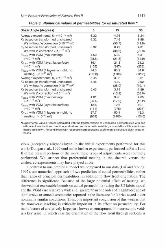
Table 8. Numerical values of permeabilities for unsaturated flow.*




(56.7)8.85



(36.3)4.81


(∗10–10 m2)4.50

(28.8)5.80

(21.8)5.31


(∗10–10 m2)16.1(155)

21.3(347)

21.2(236)


74.3(1080)

85.9(1700)

84.6(1260)



(28.0)2.92



(10.2)1.59


(∗10–10 m2)4.01

(26.4)3.96

(17.9)4.05


(∗10–10 m2)12.6(131)

12.6(275)

12.1(235)


57.7(959)

50.4(1400)

48.3(1240)

*Experimental values, values calculated with the transformation of unsheared permeabilities with andwithout volume fraction correction, and values calculated with variable gap model for all 3 cases inves-tigated are shown. Percent errors with respect to corresponding experimental value are given in paren-theses.

also critical. Our fundamental models predicted these with good accuracy.This work suggests that the time-consuming bench-scale permeability data-

base approach be supplanted by improved fabric models for low-pressure pro-cesses. Clearly, the effects of capillarity are small in such cases, as shown by thegood agreement here even for intratow permeability neglected (and validated withmore detailed simulations as well at the tow level).

An artifact of use of the present VGM, or variable gap model, is the irregularityin the calculated permeability curves. This is a result of the 1D nature of the calcu-lation: instead of flow being allowed to meet transverse to the direction studied,flow proceeds in 1D. In a real setting, the melding of flow fronts moving radiallyoutward would significantly smooth the flow pattern. Work here suggests that 2Dflow models may actually be unnecessary, however, for simple cases, in favor ofcareful consideration of how to calculate critical angles.

NOMENCLATURE

ai thickness of equivalent channel at either end (i = 1,2)A distance between either ellipse focus and y axisb half of the distance between infinitely long platesc Kozeny constant

Ca capillary numberd diameter of a tube for circular Poiseuille flowD sum of distances between any point on ellipse and two foci

DE equivalent wetted diameterF shape factor for equivalent wetted diameterFi external body forceg gravitational acceleration

2h thickness of a fabric layerK permeability

KX axial permeabilityKZ transverse permeabilityKit tow permeability

Krep representative permeabilityLsect length of a complete or completed cross-section

N number of points on ellipseP pressure

∇P pressure gradientPc capillary pressure

(Pi, Qi) ith data pointrf fiber radius

rfA micro-front radiusr1A tow radii


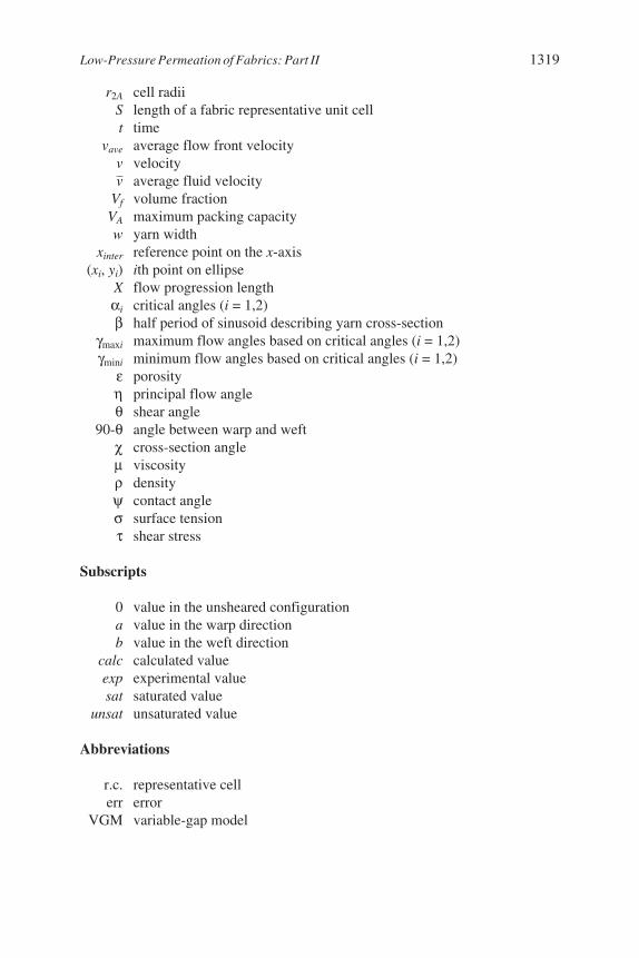
r2A cell radiiS length of a fabric representative unit cellt time

vave average flow front velocityv velocityv average fluid velocity

Vf volume fractionVA maximum packing capacityw yarn width

xinter reference point on the x-axis(xi, yi) ith point on ellipse

X flow progression lengthαi critical angles (i = 1,2)β half period of sinusoid describing yarn cross-section

γmaxi maximum flow angles based on critical angles (i = 1,2)γmini minimum flow angles based on critical angles (i = 1,2)

ε porosityη principal flow angleθ shear angle

90-θ angle between warp and weftχ cross-section angleµ viscosityρ densityψ contact angleσ surface tensionτ shear stress

Subscripts

0 value in the unsheared configurationa value in the warp directionb value in the weft direction

calc calculated valueexp experimental valuesat saturated value

unsat unsaturated value

Abbreviations

r.c. representative cellerr error

VGM variable-gap model


ACKNOWLEDGEMENTS

The authors gratefully acknowledge support for this project from the U.S.Army TACOM, General Motors, the NSF SIUCRC on Low Cost, High SpeedPolymer Composite Processing, and a National Science Foundation PECASEgrant. Support for FDD from a François-Xavier Bagnoud fellowship (Departmentof Aerospace Engineering, University of Michigan) is also gratefully acknowl-edged.

REFERENCES

Adams, K.L. and L. Rebenfeld. 1991. “Permeability Characteristics of Multilayer Fiber Reinforce-ments. Part I: Experimental Observations,” Polymer Composites, Vol. 12, No. 3, pp. 179–185.

Adams, K.L. and L. Rebenfeld. 1991. “Permeability Characteristics of Multilayer Fiber Reinforce-ments. Part II: Theoretical Model,” Polymer Composites, Vol. 12, No. 3, pp. 186–190.

Ahn, K.J., J.C. Seferis, and J.C. Berg. 1991. “Simultaneous Measurements of Permeability and Capil-lary Pressure of Thermosetting Matrices in Woven Fabric Reinforcements,” Polymer Composites,Vol. 12, No. 3, pp. 146–152.

Ambrosi, D. and L. Preziosi. 1998. “Modeling Matrix Injection through Elastic Porous Preforms,” Com-posites Part A, Vol. 29, Nos. 1–2, pp. 5–18.

Batchelor, G.K. 1967. An Introduction to Fluid Dynamics, Cambridge: Cambridge University Press.Berdichevsky, A.L. and Z. Cai. 1993. “Preform Permeability Predictions by Self-Consistent Method

and Finite Element Simulation,” Polymer Composites, Vol. 14, No. 2, pp. 132–143.Binétruy C., B. Hilaire, and J. Pabiot. 1998. “Tow Impregnation Model and Void Formation Mechanisms

during RTM,” Journal of Composite Materials, Vol. 32, No. 3, pp. 223–245.Blake, F.C. 1922. “The Resistance of Packing to Fluid Flow,” Transactions of the American Institute of

Chemical Engineers, Vol. 14, pp. 415–421.Bruschke, M.V. and S.G. Advani. 1990. “A Finite Element/Control Volume Approach to Mold Filling in

Anisotropic Porous Media,” Polymer Composites, Vol. 11, No. 6, pp. 398–405.Bruschke, M.V. and S.G. Advani. 1993. “Flow of Generalized Newtonian Fluids across a Periodic Array

of Cylinders,” Journal of Rheology, Vol. 37, No. 3, pp. 479–498.Cai, Z. and A.L. Berdichevsky. 1993. “An Improved Self-Consistent Method for Estimating the

Permeability of a Fiber Assembly,” Polymer Composites, Vol. 14, No. 4, pp. 314–323.Carman, P.C. 1937. “Fluid Flow through Granular Beds,” Transactions of the Institution of Chemical

Engineers (London), Vol. 15, pp. 150–156.Chan, A.W., D.E. Larive, and R.J. Morgan. 1993. “Anisotropic Permeability of Fiber Preforms:

Constant Flow Rate Measurement,” Journal of Composite Materials, Vol. 27, No. 10, pp.996–1008.

Chang, C.-Y. and L.-W. Hourng. 1998. “Numerical Simulation for the Transverse Impregnation in ResinTransfer Molding,” Journal of Reinforced Plastics and Composites, Vol. 17, No. 2, pp. 165–182.

Chang, C.-Y., L.-W. Hourng, and C.-J. Wu. 1998. “Numerical Study on the Capillary Effect of ResinTransfer Molding,” Journal of Reinforced Plastics and Composites, Vol. 16, No. 6, pp. 566–586.

Coulter, J.P. and S.I. Guceri. 1988. “Resin Transfer Molding: Process Review, Modeling and ResearchOpportunities,” Proceedings of Manufacturing International ’88, Atlanta, GA, pp. 79–86.

Darcy, H. 1856. Les Fontaines Publiques de la Ville de Dijon, Paris: Dalmont.Dungan, F.D. 2000. “Investigation of Microscale Flow Phenomena in Determining Permeabilities of

Fabrics for Composites.” Ph.D. Thesis. University of Michigan.Dungan, F.D., M.T. Senoguz, A.M. Sastry, and D.A. Faillaci. 1999. “On the Use of Darcy Permeability

in Sheared Fabrics,” Journal of Reinforced Plastics and Composites, Vol. 18, No. 5, pp. 472–484.


Dungan, F.D., M.T. Senoguz, A.M. Sastry, and D.A. Faillaci. 2001. “Simulations and Experiments onLow-Pressure Permeation of Fabrics: Part I—3D Modeling of Unbalanced Fabrics,” Journal ofComposite Materials, Vol. 35, No. 14, pp. 1250–1284.

FLUENT. 1998. FLUENT 5 User’s Guide Volume 1.Lebanon, NH: Fluent Inc.Gauvin, R., F. Trochu, Y. Lemenn, and L. Diallo. 1996. “Permeability Measurement and Flow Simula-

tion through Fiber Reinforcement,” Polymer Composites, Vol. 17, No. 1, pp. 34–42.Gebart, B.R. 1992. “Permeability of Unidirectional Reinforcements for RTM,” Journal of Composite

Materials, Vol. 26, No. 8, pp.1100–1133.Hourng, L.-W. and C.-Y. Chang. 1998. “The Influence of Capillary Flow on Edge Effect in Resin

Transfer Molding,” Journal of Reinforced Plastics and Composites, Vol. 17, No. 1, pp. 2–25.Ismail, Y.M. and G.S. Springer. 1997. “Interactive Simulation of Resin Transfer Molding,” Journal of

Composite Materials, Vol. 31, No. 10, pp. 954–980.Kolodziej, J.A., R. Dziecielak, and Z. Konczak. 1998. “Permeability Tensor for Heterogeneous Porous

Medium of Fibre Type,” Transport in Porous Media, Vol. 32, pp. 1–19.Kozeny, J. 1927. “Ueber Kapillare Leitung des Wassers im Boden,” Sitzungsberichte, Akademie der

Wissenschaften in Wien, Vol. 136, pp. 271–301.Kundu, P.K. 1990. Fluid Mechanics, San Diego: Academic Press.Lai, C.-L. and W.-B. Young. 1997. “Model Resin Permeation of Fiber Reinforcements after Shear De-

formation,” Polymer Composites, Vol. 18, No. 5, pp. 642–648.Lekakou, C. and M.G. Bader. 1998. “Mathematical Modeling of Macro and Micro-Infiltration in Resin

Transfer Molding (RTM),” Composites Part A, Vol. 29A, pp. 29–37.Lin, M., H.T. Hahn, and H. Huh. 1998. “A Finite Element Simulation of Resin Transfer Molding Based

on Partial Nodal Saturation and Implicit Time Integration,” Composites Part A, Vol. 29, Nos. 5–6,pp. 541–550.

Martin, G.Q. and J.S. Son. 1986. “Fluid Mechanics of Mold Filling for Fiber Reinforced Plastics,”Proceedings of the Second Conference on Advanced Composites, 18–20 November 1986,Dearborn, MI, pp. 149–157.

Mogavero, J. and S.G. Advani. 1997. “Experimental Investigation of Flow through Multi-LayeredPreforms,” Polymer Composites, Vol. 18, No. 5, pp. 649–655.

Parnas, R.S., K.M. Flynn, and M.E. Dal-Favero. 1997. “A Permeability Database for CompositesManufacturing,” Polymer Composites, Vol. 18, No. 5, pp. 623–633.

Pillai, K.M. and S.G. Advani. 1998. “Numerical Simulation of Unsaturated Flow in Woven FiberPreforms during the Resin Transfer Molding Process,” Polymer Composites, Vol. 19, No. 1, pp.71–80.

Rudd, C.D., A.C. Long, P. McGeehin, and P. Smith. 1996. “In-Plane Permeability Determination forSimulation of Liquid Composite Molding of Complex Shapes,” Polymer Composites, Vol. 17, No.1, pp. 52–59.

Sastry, A.M. 2000. “Impregnation and Consolidation Phenomena,” Vol. 2, Ch. 18 in ComprehensiveComposite Materials, A. Kelly and C. Zweben (eds), Elsevier.

Scheidegger, A.E. 1974. The Physics of Flow through Porous Media, Toronto: University of TorontoPress, p. 58.

Shih, C.H. and L.J. Lee. 1998. “Effect of Fiber Architecture on Permeability in Liquid CompositeMolding,” Polymer Composites, Vol. 19, No. 5, pp. 626–639.

Skartsis, L., B. Khomami, and J.L. Kardos. 1992. “Resin Flow through Fiber Beds, Part I: Review ofNewtonian Flow through Fiber Beds,” Polymer Engineering and Science, Vol. 32, No. 4, pp.221–230.

Skartsis, L., B. Khomami, and J.L. Kardos. 1992. “Resin Flow through Fiber Beds, Part II: Numericaland Experimental Studies of Newtonian Flow through Ideal and Actual Fiber Beds,” Polymer En-gineering and Science, Vol. 32, No. 4, pp. 231–239.

Skartsis, L., B. Khomami, and J.L. Kardos. 1992. “The Effect of Capillary Pressure on the Impregnationof Fibrous Media,” SAMPE Journal, Vol. 28, No. 5, pp. 19–24.


Smith, P., C.D. Rudd, and A.C. Long. 1997. “The Effect of Shear Deformation on the Processing andMechanical Properties of Aligned Reinforcements,” Composites Science and Technology, Vol. 57,pp. 327–344.

Song, B., A. Bismarck, R. Tahhan, and J. Springer. 1998. “A Generalized Drop Length-Height Methodfor Determination of Contact Angle in Drop-on-Fiber Systems,” Journal of Colloid and InterfaceScience, Vol. 197, No. 1, pp. 68–77.

Song, Y., W. Chui, J. Glimm, B. Lindquist, and F. Tangerman. 1997. “Applications of Front Tracking tothe Simulation of Resin Transfer Molding,” Computers and Mathematics with Applications, Vol.33, No. 9, pp. 47–60.

Van der Westhuizen, J. and J.P. Du Plessis. 1996. “An Attempt to Quantify Fibre Bed PermeabilityUtilizing the Phase Average Navier-Stokes Equation,” Composites Part A, Vol. 27A, pp. 263–269.

Wagner, H.D. 1990. “Spreading of Liquid Droplets on Cylindrical Surfaces: Accurate Determination ofContact Angle,” Journal of Applied Physics, Vol. 67, No. 3, pp. 1352–1355.

Wang, C.Y. 1996. “Stokes Flow through an Array of Rectangular Fibers,” International Journal ofMultiphase Flow, Vol. 22, No. 1, pp. 185–194.

Williams, J.G., C.E.M. Morris, and B.C. Ennis. 1974. “Liquid Flow through Aligned Fiber Beds,”Polymer Engineering and Science, Vol. 14, No. 6, pp. 413–419.

Young, W.-B. 1996. “The Effect of Surface Tension on Tow Impregnation of Unidirectional FibrousPreform in Resin Transfer Molding,” Journal of Composite Materials, Vol. 30, No. 11, pp.1191–1209.

Young, W.-B. and S.F. Wu. 1995. “Permeability Measurement of Bidirectional Woven Glass Fibers,”Journal of Reinforced Plastics and Composites, Vol. 14, pp. 1108–1120.


Documents

Simulations and Experiments on Low-Pressure Permeation of