SIMULATION OF SHOT IMPACTS FOR THE M1A1 TANK … · SIMULATION OF SHOT IMPACTS FOR THE ... all are used for design evaluation. ... DYNAMIC INDEXING OF GUN TUBES AND TEST RESULTS The

AD

TECHNICAL REPORT ARCCB-TR-00009

SIMULATION OF SHOT IMPACTS FOR THE M1A1 TANK GUN

RONALD GAST STEVEN MORRIS

MARK COSTELLO

JUNE 2000

US ARMY ARMAMENT RESEARCH, DEVELOPMENT AND ENGINEERING CENTER

CLOSE COMBAT ARMAMENTS CENTER BENET LABORATORIES

WATERVLIET, N.Y. 12189-4050

APPROVED FOR PUBLIC RELEASE; DISTRIBUTION UNLIMITED

mGWAUTYwm(msD 4 20000705 071

DISCLAIMER

The findings in this report are not to be construed as an official Department of the

Army position unless so designated by other authorized documents.

The use of trade name(s) and/or manufacturer(s) does not constitute an official

endorsement or approval.

DESTRUCTION NOTICE

For classified documents, follow the procedures in DoD 5200.22-M, Industrial

Security Manual, Section 11-19, or DoD 5200.1-R, Information Security Program

Regulation, Chapter DC

For unclassified, limited documents, destroy by any method that will prevent

disclosure of contents or reconstruction of the document.

For unclassified, unlimited documents, destroy when the report is no longer

needed. Do not return it to the originator.

4. TITLE AND SUBTITLE

SIMULATION OF SHOT IMPACTS OR THE Ml Al TANK GUN

6. AUTHOR(S)

lonald Gast, Steven Morris, and dark Costello (Oregon State University, Corvallis, OR)

7. PERFORMING ORGANIZATION NAME(S) AND ADDRESS(ES)

J.S. Army ARDEC Jenet Laboratories, AMSTA-AR-CCB-O iVatervliet, NY 12189-4050

REPORT DOCUMENTATION PAGE Form Approved

OMB No. 0704-0188

Public reporting burden for this collection of information is estimated to average 1 hour per response, including the time for reviewing instructions, searching existing data sources, gathering and maintaining the data needed, and completing and reviewing the collection of information. Send comments regarding this burden estimate or any other aspect of this collection of information, including suggestions for reducing this burden, to Washington Headquarters Services. Directorate for Information Operations and Reports, 1215 Jefferson Davis Highway, Suite 1204, Arlington, VA 22202-4302. and to the Office of Management and Budget, Paperwork Reduction Project (0704-0188). Washington, DC 20503.

1. AGENCY USE ONLY (Leave blank) 2. REPORT DATE June 2000

3. REPORT TYPE AND DATES COVERED Final

5. FUNDING NUMBERS

AMCMS No. 6226.24.H191.1

8. PERFORMING ORGANIZATION REPORT NUMBER

ARCCB-TR-00009

9. SPONSORING/MONITORING AGENCY NAME(S) AND ADDRESS(ES)

J.S. Army ARDEC -lose Combat Armaments Center 'icatinny Arsenal, NJ 07806-5000

10. SPONSORING /MONITORING AGENCY REPORT NUMBER

11. SUPPLEMENTARY NOTES 'resented at the 9th U.S. Army Gun Dynamics Symposium, McLean, VA, 17-19 November 1998. *ublished in proceedings of the symposium.

12a. DISTRIBUTION/AVAILABILITY STATEMENT

approved for public release; distribution unlimited.

12b. DISTRIBUTION CODE

13. ABSTRACT (Maximum 200 words)

>Jever has the need for simulation in design of components been more acute. Today's business environment requires innovative thinking in >roduct development, especially for the *big-ticket' ordnance items such as main battle tanks and armament. The manufacturing costs of these terns and related components prohibit use of the classical method of product development, which includes initial design, prototype manufacture, lystem testing, and redesign. The answer lies in the use of virtual performance simulation to assess a system's response before any hardware s manufactured. Up-front costs are greatly reduced since the system components reside in virtual space, allowing for rapid electronic design foanges and optimization by simulation rather than iterative testing of costly hardware.

3ne must not be overly enamored by the power and function of the simulation tools. They are just mathematical models written by mere nortals, the execution of which closely mimics nature but does not actually reproduce it. Ultimately, these simulations need to be validated jefore one becomes comfortable in their use. There are various ways to validate a simulation code. First, one may use dedicated and controlled ests void of extraneous noise to establish relational characteristics among a few test variables. The results may then be directly compared to imulations, with validation achieved when output closely matches the test data. The second method involves comparing simulated results to nherently noisy field-generated test data. The best one may expect to achieve from this type of validation is trends in the responses relative o variations in the system parameters. It is the purpose of this report to validate a coupled simulation package for the accuracy assessment of arge caliber weapons. The simulation packages include SIMBAD, a finite element gun dynamics code, and BOOM, a projectile flight dynamics :ode. These two models have been coupled so that the output of SIMBAD is the input to BOOM. Simulated results are compared to field- jenerated accuracy firings for the Ml Al tank, thus method two validation was used to assess the worth of this endeavor.

14. SUBJECT TERMS

3un Dynamics, Tank Gun Accuracy, Flexural Body Dynamics, ixterior Ballistics, Ml Al Tank, Kinetic Energy Projectile

15. NUMBER OF PAGES

.42 16. PRICE CODE

17. SECURITY CLASSIFICATION OF REPORT

tJNCLASSLFIED

18. SECURITY CLASSIFICATION OF THIS PAGE

UNCLASSIFIED

19. SECURITY CLASSIFICATION OF ABSTRACT

UNCLASSIFIED

20. LIMITATION OF ABSTRACT

UL

NSN 7540-01-280-5500 Standard Form 298 (Rev Prescribed by ANSI Std. Z39-18 298-102

2-89)

TABLE OF CONTENTS Page

INTRODUCTION 1

DYNAMIC INDEXING OF GUN TUBES AND TEST RESULTS 2

Characteristics of the DIT Profile 2 Conduction of the DIT Test. 3 Results of the DIT Test 3

DESCRIPTION OF ANALYSIS MODELS . 4

Simulation of Barrel Dynamics (SIMBAD) Gun Vibration Model 4 BOOM - A Six Degree-of-Freedom Exterior Ballistics Code 5 Integration of SIMBAD and BOOM 5

CONDUCTION OF THE ANALYSIS 5

Bore Centerline Profile Estimation 6 Projectile Specifications 8 Gun Mount Specifications : 8 Ballistic Data 9 Aiming of the Weapon 10 Values for the Uncertain Analysis Parameters 10

RESULTS OF ANALYSIS 11

RECOMMENDATIONS AND CONCLUSIONS 12

REFERENCES 15

LIST OF ILLUSTRATIONS

1. Average centers of impact for select tubes in DIT test 16

2. Curve fitting process for data processing errors in measurement 17

3. Chi-square method for fitting data with measurement error 18

4a. Vertical profile and curvature for Tube #4098 19

4b. Vertical profile and curvature for Tube #4100 20

l

4c. Vertical profile and curvature for Tube #4102 21

4d. Vertical profile and curvature for Tube #4104 22

4e. Vertical profile and curvature for Tube #4106 23

4f. Vertical profile and curvature for Tube #4988 24

4g. Vertical profile and curvature for Tube #4990 25

4h. Vertical profile and curvature for Tube #4992 26

4i. Vertical profile and curvature for Tube #4994 27

4j. Vertical profile and curvature for Tube #4996 28

5a. Horizontal profile and curvature for Tube #4098 29

5b. Horizontal profile and curvature for Tube #4100 30

5c. Horizontal profile and curvature for Tube #4102 31

5d. Horizontal profile and curvature for Tube #4104 ; 32

5e. Horizontal profile and curvature for Tube #4106 33

5f. Horizontal profile and curvature for Tube #4988 34

5g. Horizontal profile and curvature for Tube #4990 35

5h. Horizontal profile and curvature for Tube #4992 36

5i. Horizontal profile and curvature for Tube #4994 37

5j. Horizontal profile and curvature for Tube #4996 38

6. Schematic of kinetic energy round in gun bore 39

7. Schematic of Ml Al gun mount and cannon 40

8a. Comparison of results for Tube #4098 41

8b. Comparison of results for Tube #4100 41

ii

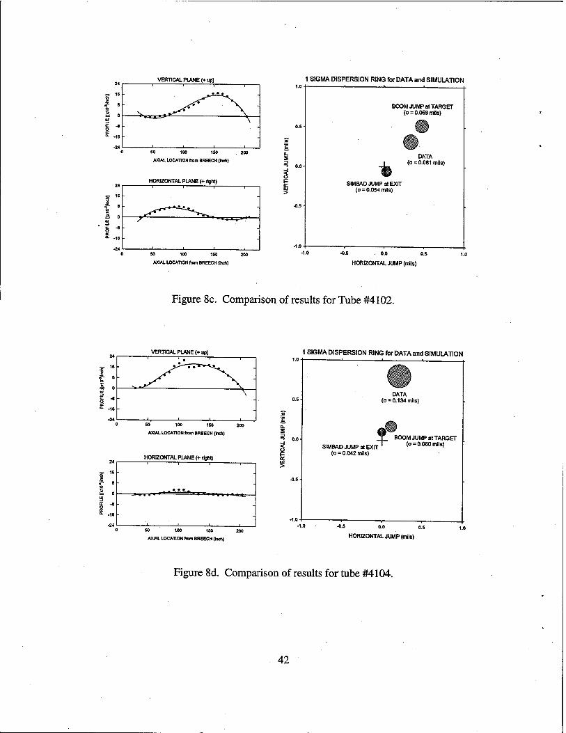
8c. Comparison of results for Tube #4102 42

8d. Comparison of results for Tube #4104 42

8e. Comparison of results for Tube #4106 43

8f. Comparison of results for Tube #4988 43

8g. Comparison of results for Tube #4990 44

8h. Comparison of results for Tube #4992 .- 44

8i. Comparison of results for Tube #4994 45

8j. Comparison of results for Tube #4996 45

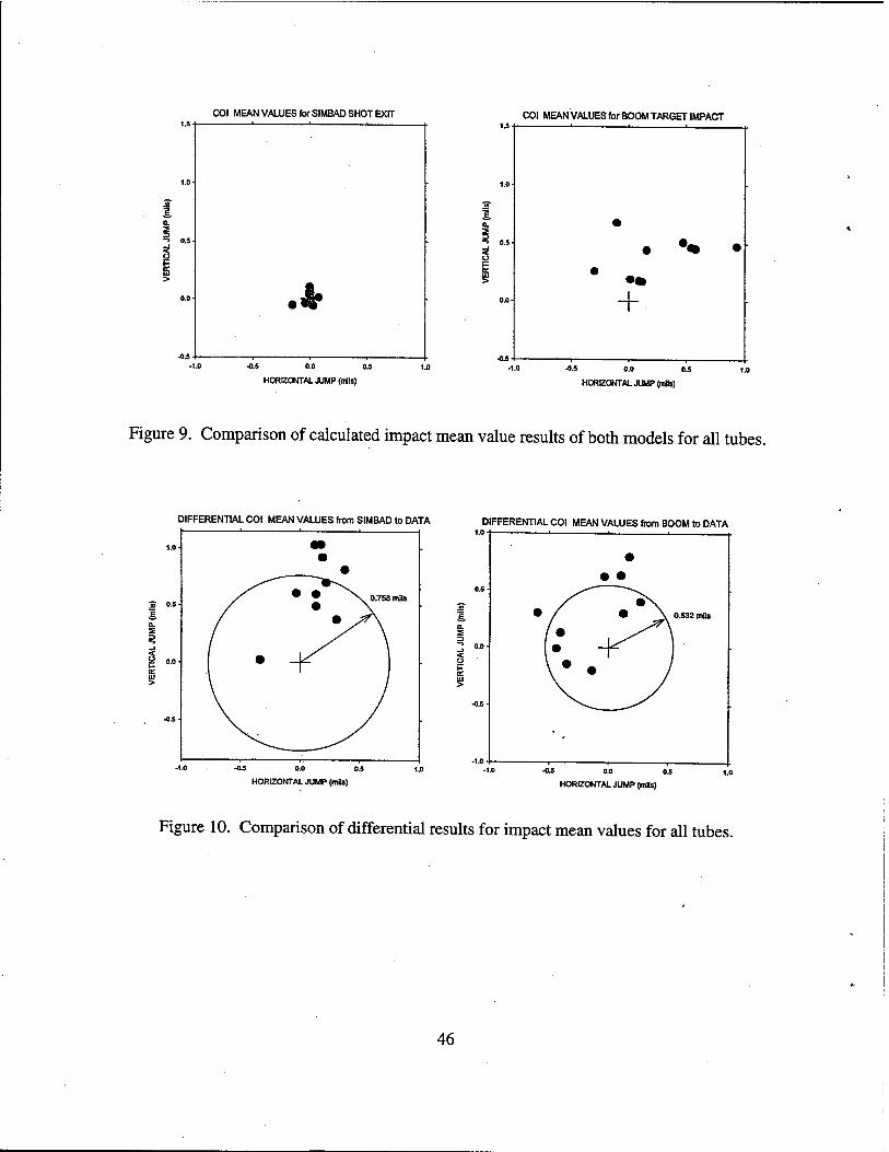
9. Comparison of calculated impact mean value results of both models for all tubes 46

10. Comparison of differential results for impact mean values for all tubes 46

in

INTRODUCTION

Never has the need for simulation in design of systems been more acute. Today's financial/philosophical environment requires innovative thinking in the business of product development, especially for the 'big-ticket' ordnance items such as main battle tanks and armament. The manufacturing costs of these items and related components prohibit use of the classical method of product development. This method, which is an iterative process, includes initial design, prototype manufacture, system testing, and redesign. As a result, considerable time and money is invested for manufacturing and testing of prototype components. We need to rethink the use of this loop if we are to remain competitive and reduce the cost of development. The answer lies in the use of a new class of electronic computational product development functions, namely, virtual performance simulation (VPS), validation by component testing (VCT), and scale model manufacture by stereo lithographic fabrication (STL). By using these methods, prototype manufacture and physical testing phases are minimized and replaced by STL and VPS. Costs are greatly reduced since the system components reside in virtual space, allowing for rapid electronic design changes and performance ratings by simulation rather than physical testing. In the end, hardware must eventually be manufactured and tested; however, this may be done after a considerable number of 'excursions' through VPS and STL.

At the heart of VPS resides various modeling and simulation programs, some of which are legacy codes developed by system designers and others are commercial codes that may have been modified for specific uses. In any event, all are used for design evaluation. Ultimately, these models and simulations need validation to achieve a level of comfort in their use. There are various ways to validate a simulation code. First, one may use dedicated and controlled tests void of extraneous noise to establish relational characteristics among a few test variables. The results may then be compared to simulations produced using the same range of independent (design) variables. Validation is achieved when the output response of the two (test and model) nearly produces the same results. The second method involves the use of field-generated data to compare with results of simulations. The field data may contain extraneous 'noise,' as well as unknown or unmeasurable system features that affect the system's response. The best one may expect to achieve from this type of validation is trends in the responses relative to variations in the system parameters. This is a type differential analysis and is more prevalent for modeling full operational systems, such as fielded ordnance weapons. As the controllable design variables are changed, results yield response trends rather than accurate reproduction of the system's performance.

It is the purpose of this report to validate a coupled simulation package for accuracy assessment of a fielded tank weapon, namely, the Ml Al tank and its main armament, the M256 120-mm cannon. Since the data to be used have been generated during field firings, of the weapon, the second method of validation applies. The importance of simulating the accuracy of this weapon lies in the current trend of establishing gun jump correction factors. The 'fleet zero' method is used and basically corrections for an entire fleet are determined by firing accuracy tests using only a few tanks and gun tubes. Refiring the tank after each retubing is considered too costly and has been abandoned. However, test results for this system reveal that shotfall patterns

1

are strongly a function of the individual gun tubes. Every gun tube that has been manufactured has its own signature regarding its dynamic response during firing and more importantly the impartation of the projectile kinematic state upon exit from the muzzle. To confirm this, factual evidence will be developed later in this report. It seems reasonable that if accurate simulations of gun accuracy could predict the shotfall patterns of individual gun tubes, then jump correction adjustments could be applied to the 'fleet zero' correction. This should be the ultimate goal of all gun dynamics studies.

DYNAMIC INDEXING OF GUN TUBES AND TEST RESULTS

The M256 cannon has characteristics that cause transverse gun vibrations during firing. One of these is due to the offset breech (about 1.25 inches below centerline of bore). As the gun recoils, this offset mass produces an inertia couple that transmits a vibration wave along the tube's axis overtaking the projectile and disturbing the muzzle before shot exit. Also, as the projectile travels along the bore, interactive loads develop between tube and projectile causing additional vibrations of both. Upon exit, the intended direction of the round has been compromised. The effect could be mitigated as Reference 1 suggests by specifying a characteristic bore profile, which minimizes the vibratory nature of projectile/tube/offset mass interaction. Based upon dynamic analysis, a tube possessing this 'optimum' profile would vibrate in such a manner as to provide a relatively straight path (in a global sense) for the projectile to follow. This would minimize side loadings and projectile cross-axis deflections rendering a benign entrance into free flight void of any asymmetric kinematic excitations. The profile that minimizes this side loading is termed the "optimum profile." The method of implementing this feature is called dynamic indexing of the tube (DIT).

Characteristics of the PIT Profile

The optimum profile is dependent upon both projectile and charge temperature; the HEAT round has its own optimum profile, as well as another for the KE round. Since the KE round is considered critical, the optimum profile is assumed to mean optimum for the KE round. The profile has the following characteristics. In the vertical plane, the optimum profile resembles a sine wave having a wavelength about 25% greater than the tube length and a magnitude of about 0.015 inch. In the horizontal plane, the optimum profile is a negative sine wave of a wavelength equal to the tube length and a magnitude of about 0.002 inch. It was not suggested that tubes be manufactured to this profile, but rather orient their top vertical centerlines such that the bore profiles (horizontal and vertical) best match the optimums. A least squares technique and a computer algorithm were incorporated into the manufacturing process. Normally, the standard method of tube indexing (STD) is to orient the top vertical centerline of the gun such that the plane of greatest bending is vertical and the tube's muzzle points up. This method tends to minimize curvature due to normal gravity droop when a cannon is mounted in its vehicle.

Conduction of the PIT Test

In attempting to verify the DU claim, an extensive test was performed during the early 1990s (ref 2). A considerable number of new M256 gun tubes were specifically manufactured for the test. Of these, a number were dynamically indexed, whereas the rest were indexed according to the standard method. The cannons were mounted on Ml Al vehicles and accuracy tests were performed. Both HEAT and KE rounds conditioned to various temperatures were used in the test. Each tube fired three rounds using each round type and condition temperature. The centers of impact (COI) and target impact dispersion (TID) were the primary data reported. Reference 2 contains all of these data.

For the study to be reported herein, a portion of the unclassified data will be used. The goal is not to verify dynamic indexing, but rather an attempt to validate a dynamic, kinematic, and accuracy simulation of the Ml Al fielded weapon's system for a representative sample of M256 gun tubes. It is felt that the profile characteristic of each tube—either indexed to the optimum or standard method—has an effect upon the projectile's "ride" down the bore and its subsequent jump upon disengagement. One round type conditioned to ambient temperature was chosen for the modeling. Rounds of this type were fired through ten gun tubes. Five were indexed by DIT, whereas the remaining were indexed by STD. Profile data were received from Watervliet Arsenal's Quality Assurance Branch and used to establish the "best" polynomial fit for each tube. The fitting process will be explained later in this report.

Results of the PIT Test

Figure 1 presents the average COI values for the ten tubes tested. On the chart, the inverted triangular symbols refer to the PIT tubes, while the upright triangular symbols refer to the STP tubes. With the exception of one flier for the PIT group, the remaining four responses seem to reside in close proximity on the plot, whereas the five from the STP group reside at a different location. The basic idea of dynamic indexing is to reduce the tube to tube variation in impact location and dispersion. But as is concluded in Reference 2, neither has the dispersion been significantly reduced nor has the impact location remained constant. However, as the COI data indicate, the PIT tubes brought the impact points closer to the point of aim, which is at the cross hairs. Additionally, the PIT tubes were not manufactured to the optimum profile, rather the tubes' natural profile was best aligned to the optimum. (There is also some controversy as to the processing sequence after the index plane was found.)

The idea of dynamic indexing versus standard indexing, profile samples, and partial results of a PIT test have been presented in this section. In the next section, the gun dynamics and exterior flight simulation models will be discussed, and relevant data pertaining to their use will be developed.

DESCRIPTION OF ANALYSIS MODELS

Two analytical computer codes have been used to determine the trajectory of a projectile's flight path, namely, SMBAD for in-bore dynamics and BOOM for free external flight to the target.

Simulation of Barrel Dynamics (SIMBAD) Gun Vibration Model

Dr. David Bulman developed the SIMBAD model in Great Britain while he was a faculty member at the Royal Military College of Science. It is a quick running, finite element code that employs beam elements for the gun tube and a variety of options for modeling the projectile, mount, and cradle. SIMB AD was recently purchased by Benet (in source code form) and has been used exclusively for gun dynamics modeling. Dr. Bulman has continually added functionality to the code enhancing Benet Lab's capability to perform gun dynamics studies for experimental purposes or within the design loop of a gun development program.

The gun tube is defined using either the Euler-Bernoulli or Timoshenko formulation. The projectile and sabot may have its own finite element representation or simply a solid shot coupled to the tube through elastic driving bands. The mount and cradle may also be modeled in finite elements or represented simply using a lumped spring and mass. A direct fixed time-step integration method'is employed to solve the system of differential equations. A partial list of SIMBAD applications includes:

• Evaluation of optimum dimensions for a gun tube to improve accuracy • Examination of the effect of offset masses on weapon performance • Examination of the effect that gun mounting parameters have on accuracy,

specifically: • Wheelbase and clearance • Trunnion position with respect to gun center of gravity • Recoil brake and recuperator location and performance

• Analysis of the effect that tube straightness has upon accuracy • Determination of the effect of that dimensional tolerance of the round has upon

accuracy

The program runs either interactively or through batch files of user-defined inputs. For the study conducted herein, the tube is defined using a 40-element Euler beam model and 41 nodes. The centerline profiles for the ten gun tubes used in this study have been determined using statistical methods to be described in the next section. The mount is simulated using nonlinear elastic supports to the cradle, which is considered ground. The projectile and sabot are both modeled using seven finite elements with an additional mass for the penetrator's tail fin. The sabot and gun tube are coupled at two points through linear stiffness elements using data from a static test performed in the early 1990s. A simplified sabot decompression model developed at Benet Labs further perturbs the projectile's exit kinematics. It is based upon conservation of energy, in which the asymmetric compression of the penetrator/sabot interface is

4

converted to transverse rotational energy imparted to the penetrator, thus modifying the pitch and yaw rates at exit. This level of detail is considered sufficient for our needs.

BOOM - A Six Degree-of-Freedom Exterior Ballistics Code

Dr. Mark Costello developed the BOOM code while he was a faculty member at the U.S. Military Academy. It is a rigid body dynamics/kinematics computer code used to predict the external flight path of ordnance projectiles. Benet Labs acquired the source code from the author in 1996. Although Dr. Costello transferred to Oregon State University in early 1998, he continues to upgrade the code increasing its functionality and performance. Validation studies using full-scale gun systems have been performed at the Army Research Lab and Aberbeen Proving Ground.

The projectile is described with six rigid body degrees-of-freedom comprised of three body inertial position coordinates as well as three Euler angle body attitudes. The body frame coordinate system is defined with respect to the earth's inertial reference frame. The dynamics equations are written in body frame coordinates. Dynamics and kinematics values may be expressed in either coordinate system through a series of matrix transform equations that transfer values from one system to the other. The projectile's inertia matrix may be fully populated (i.e., nine values) if the center of mass is offset from its geometric center. Externally applied forces and moments due to aerodynamic lift, drag, and gravity drive the projectile along its flight path. The aerodynamic coefficients are geometry specific and obtained empirically through flight test experiments.

Integration of SIMBAD and BOOM

An interface routine employing matrix equations was developed in which projectile kinematic values from SIMBAD exit conditions were transferred into the coordinate system used in BOOM. It proved to be a bit of a challenge, since the authors of both codes resided on different continents. However, it was eventually accomplished, thus assuring seamless passing of data from SIMBAD to BOOM.

For the studies conducted in this program, the projectile was completely balanced and the atmospheric condition was standard with no wind. Reiterating, our studies are to be of a comparative nature, therefore, much of the code's functionality was not needed.

CONDUCTION OF THE ANALYSIS

The ultimate goal of this study is to decide if the coupling of two simulation codes for predicting in-bore gun dynamics and the projectile's flight trajectory is reliable for predicting shot impact location. The means by which this may be established is to model the test conditions of the individual shots and compare the predicted shot impact locations with the test results. To accomplish this, the values of many system parameters are required as input to the models. With the exception of the relevant dimensions of the gun tubes used in the test, many of remaining

parameters were neither measured nor recorded. To deal with this problem, parametric methods of analysis will be used. Nominal values for those unknown parameters considered to be important will be selected and incremented within a reasonable range with simulations being conducted for every combination of parameters. Thus, a distribution of shot impact locations for a given gun tube will be generated. Computed and test results can then be compared on the basis of both mean value and standard deviation. In the following paragraphs, the relevant system parameters and the rationale for the selection of their range of values will be discussed.

Bore Centerline Profile Estimation

It is a well-known fact that the condition of the gun tube's centerline profile affects the in- bore vibrational response of both the tube and round (ref 3), as well as the mean impact location and dispersion of the shots fired during an accuracy test (ref 2). Therefore, in a modeling sense, an accurate method of determining the 'correct' bore profile is important. Theoretically speaking it is not the bore profile that is important, but rather the curvature of the path (i.e., second derivative of profile) that the projectile must traverse as it progresses downbore. This author and several others (refs 4,5) have pointed out the analytical effect of this. Watervliet Arsenal personnel inspected the gun tubes used in this test using normal production inspection methods. Bore profile measurements were taken using the mechanical procedure in place at that time (circa 1989). The inspection interval along the tube was approximately 0.75 feet for a total of 23 measurement stations. Profile measurements were subject to an error of approximately 0.00118 inch due to the nature of the measurement system.

The goal is to use these data for the generation of a representative 'smooth' profile, which possesses the necessary curvature information to best calculate the interactive forces between the accelerating projectile and gun tube. The means of achieving this is to generate a polynomial fit of the data using a least squares technique. For analysis purposes, the profile is approximated using the functional fit, which employs a spacing interval that is much finer than that of the raw data. These 'data' are stored in a tabular file that is used by SMB AD to set the initial locations of the .structure's nodes prior to executing in-bore gun dynamics calculations.

The statistical problem becomes one of deciding what order of polynomial to use for representing the data. Figure 2 contains a schematic of the rationale involved in the fitting process. Shown on this figure are generic measurement data, error bars, and the types of fit that may be applied. On the uppermost graph, the data with error bars and a high order polynomial fit are represented. In this fit, the functional polynomial is made to pass through each reported data point. Since the data contain measurement errors at each station, this fit is overly restrictive in that we assume that each point is truly representative of the actual condition of the profile. Conversely, on the middle graph the opposite is true. The fit here is too loose in that most of the function values fall outside of the error-bar range. The bottom graph shows a fit that is appropriate for the data and errors shown. The fitted function falls within the error bars, however, it does not pass through each point but rather meanders within error bars sometimes above and sometimes below the measured values.

The statistical method used to determine the proper order of the polynomial fit (ref 6) involves computing the Chi-squared statistic as shown in Figure 3. The Chi-squared statistic is the summation over all data points of the ratio of the difference between the measured and calculated values squared divided by the square of the measurement error. This resulting summation is compared with the degrees-of-freedom used for analysis. It is the difference between the number of data points and fit parameters (i.e., one more than the order of fit). If the statistic is much larger than the degrees-of-freedom, a poor fit results. If the statistic is much less, then the fit is too constrained. The statistic and degrees-of-freedom must be nearly the same for the fit to be suitable.

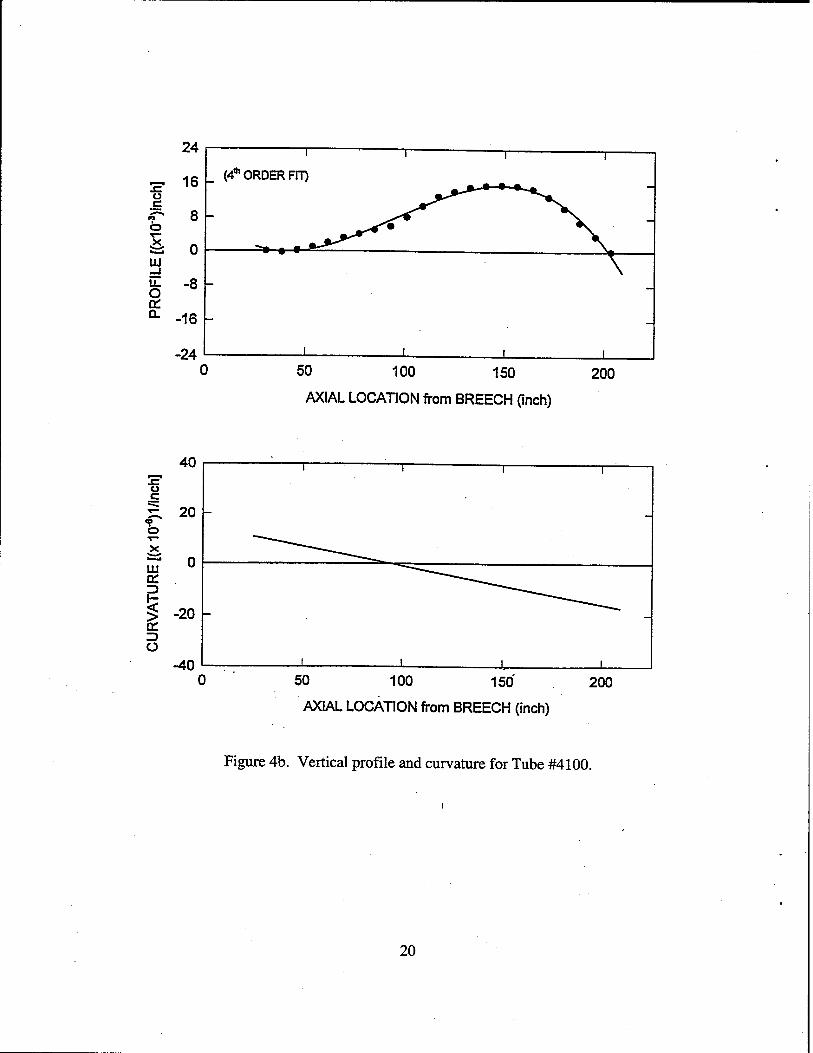
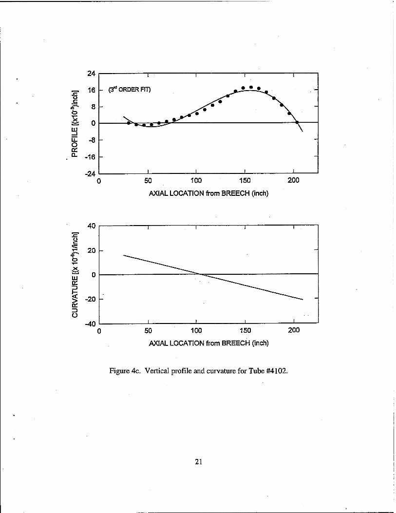
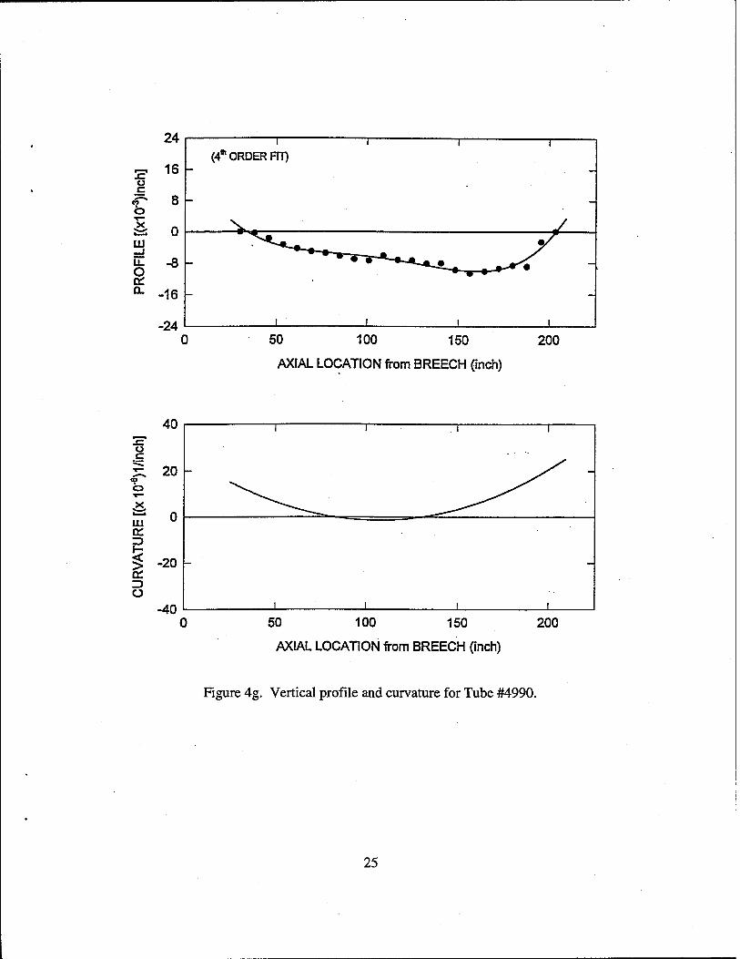
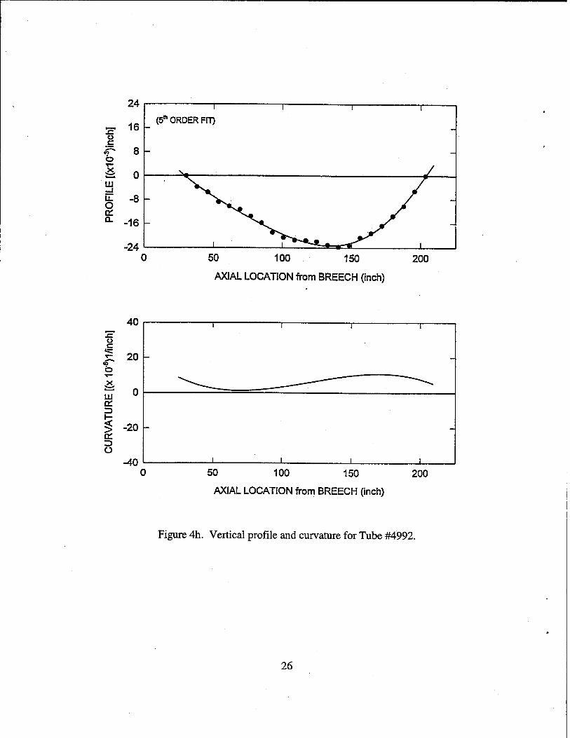
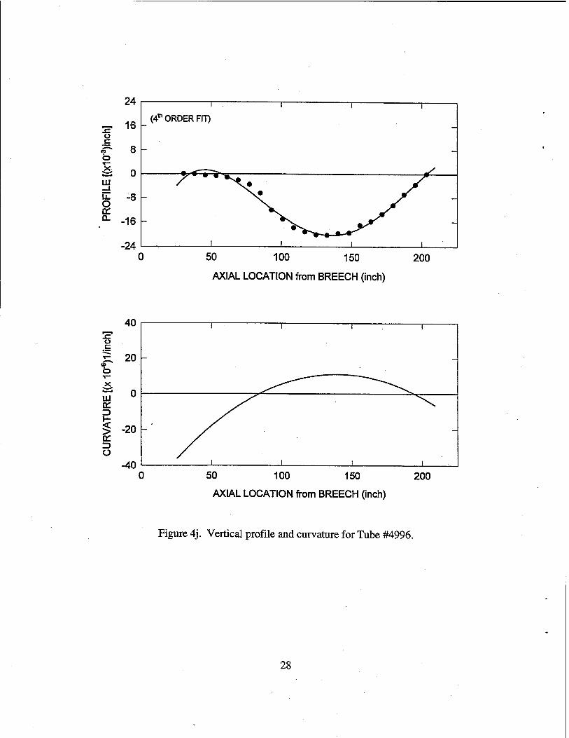
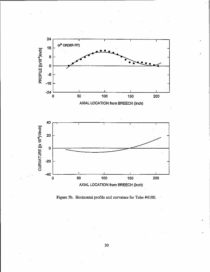
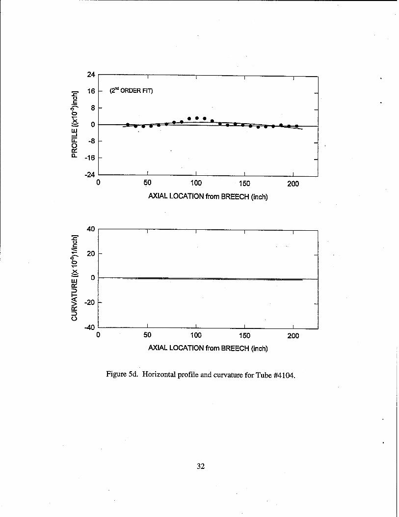
A straightforward method for determining the polynomial order does not exist; rather an iterative process must be employed as follows. Assume an order for the polynomial, generate the fit using least squares, calculate the Chi-squared statistic, and compare with the degrees-of- freedom. This process continues until the fit criteria are achieved. This method was used for generating the profile for each gun tube in the analysis. The profile data, calculated fit, and curvature derived from the second derivative of the fit for all ten tubes, are shown in Figures 4a through 4j for the vertical plane, and in Figures 5a through 5j for the horizontal plane.

Figures 4a through 4e show the vertical profile data, functional fits, and curvatures, as well as the orders of fit, for the five DIT tubes. The profile characteristics are quite similar. All five tubes tend to point down at the muzzle. Tube #4098 has the greatest deviation of 0.020 inch occurring over the last 50 inches of travel. Tube #4104 has the same amount of deviation, however, it is spread over 100 inches of travel. The remaining three tubes have deviations of lesser magnitude. The order of fit specified on the graphs represents the order of the approximating polynomial used to represent the data. For the DIT tubes, the curvature in the vertical plane tends to decrease towards the muzzle. The magnitudes near the muzzle, however, are somewhat different. For Tube #4098 the value is -40x10"6 [1/inch], whereas for #4106 muzzle curvature is only lOxlO"6 [1/inch]. Muzzle curvature for the remaining three tubes falls between these values.

Figures 4f through 4j show the vertical profile data, functional fits, and curvatures for the five STD tubes. These are similar in that the muzzle end of each points up. Tube #4992 has the greatest profile deviation of -0.024 inch, which occurs over the last 60 inches of travel. The orders of fit range from 3 to 5. Curvature values are somewhat unique. For Tubes #4988 and #4996, curvature tends to begin at -40xl0"6 [1/inch], grows to slightly above zero, and finally ends up at zero to -5xl0"6 [1/inch] at the muzzle. Tube #4990 has a curvature that is nearly a mirror image of Tubes #4988 and #4996, whereas the curvature for Tubes #4992 and #4994 is very close to zero for the entire length.

Figures 5a through 5e show the profile data, fits, and curvature values in the horizontal plane for the DIT tubes. As indicated in these plots, the orders of fit range from 2 to 5. Tubes #4100 and #4106 possess the greatest deviation of around 0.012-inch midpoint along the tube. Tube #4104 is nearly straight. Curvature signatures have no similarity. Tube #4104 has nearly zero curvature, whereas Tube #4106 has a curvature signature that bows down and achieves a

value of 40x10"6 [1/inch] at the muzzle. The curvature for Tube #4098 is nearly a mirror image ofthat of #4106. Curvatures for the remaining tubes in this group are within these bounds.

Figures 5f through 5j show the profile data, fits, and curvature values in the horizontal plane for the STD tubes. Due to the indexing technique used for these tubes, the horizontal plane possesses nearly zero profile deviation. Hence, all tubes with the exception of #4990 contain curvature responses of less than lOxlO"6 [1/inch]. The curvature response for Tube #4990 begins at -40xl0"6 [1/inch], increases to zero for about 75 inches, and then increases to 20xl0"6

[1/inch] at the muzzle. It is anticipated that very little projectile/tube interaction will occur for these tubes.

Projectile Specifications

Kinetic energy trainer rounds were used in this test, a schematic of which is shown in Figure 6. It is a multiple piece construction employing a three-petal aluminum sabot, aluminum tail fin, and low alloy steel penetrator. The nominal dimensions on the round's engineering drawings were consulted to generate the finite element analysis model for both components. Even though the sabot is flexible, SMBAD needs explicit specifications for the force/penetration data at the contacting surfaces between sabot bore riders and tube inner diameter at both the front and rear contact points. Lyon (ref 7) has conducted stiffness tests for this round and has provided experimental data for both locations. As indicated in his report, the stiffness is nonlinear for both areas. The material resistance is small during initial sabot deflection, then gradually increases as deflection becomes greater. This, of course, is quite understandable since the interaction between the sabot and tube is like a Hertzian contact situation. Resistance is light during initial penetration and builds rapidly thereafter. A second characteristic of this round is that due to its construction (three symmetrical petals of 120° including angle), the assembly stiffness is a function of the location around the sabot's periphery. For example, if the projectile is oriented such that the load is applied to the circumferential center of a petal, its stiffness is different than if the load were applied at the joint between two petals. The stiffness range around the periphery has a 15% variation from the maximum stiffness value.

Gun Mount Specifications

The most elusive modeling parameter in this gun system includes the clearances and stiffness between the recoiling cannon and its stationary mount. As with the projectile-to-tube interface, the tube-to-mount interface must be explicitly defined. The mounting specifications are characterized by nonlinear spring elements applied at the gun's mounting locations. The function representing this relationship need not be linear or continuous.

A schematic of the major components involved in the mounting of the gun is illustrated in Figure 7. Points A and B are seal locations within which the recoil fluid resides. These locations are also considered the cannon's mounting points for vibrational analysis. The spring located in this chamber compresses between the piston head and rear surface of the cradle during recoil. It provides the necessary energy to return the cannon to its in-battery position. All components

except the cradle are subject to recoil motion and the major level of transverse vibration. The adaptor, which has an internal profile closely matching the gun tube's outer profile, is held in place by the bearing that drives the adaptor inward, thus engaging the tube's outer surface. The king nut, which is threaded to the outer surface of the tube, provides the clamping force to maintain the bearing/adaptor assembly to the tube. The thrust nut is the link that marries together all of the recoiling components. It has an internal thread that engages a mating thread on the outer diameter of the bearing. When tightened, the load pulls the cannon and piston forward through the bearing, king nut, tube, and breech threads. The cradle is assumed to be grounded along the face at the shoulder located just forward of the fluid and spring chamber. See feature C in the figure. This represents the forward end of the rotor and is considered to be grounded with respect to the vibrating cannon.

By examining the relevant component drawings, the range of clearances between recoiling and stationary parts in the assembly is 0.005 to 0.010 inch at point A and 0.001 to 0.011 inch at point B. When the cannon is within the clearance, its transverse motion will be unopposed by any external loads except its own inertia. However, when the king nut is tightened to its preload specification, the clearance between recoiling and nonrecoiling components decreases considerably. Wilkerson has measured these clearance values and has determined that at most 0.002 inch is realizable at either location (ref 8).

A twofold approach was employed to determine the structural resistance during contact. Since the cradle is assumed to be grounded" along its mid-axial location (see feature C in Figure 4), both the breech and the muzzle end resemble short cantilever beams. Stiffness values for this type of structure are well documented in textbooks on deformable materials, and for this mount's dimensions, the stiffness value would be on the order of several million pounds per inch. A stiffness value of this magnitude is grossly inaccurate, yielding an extremely 'stiff mathematical system along with all of its numerical difficulties. Therefore, an alternate type of response, namely Hertzian contact, was developed and applied in series with the beam model. Hertzian contact deals with the local microscopic levels of deformation and contact stress between elastic components of various geometries. Details and applications of this method are described in Reference 9. Unlike the beam model whose stiffness is constant regardless of the level of deformation, the interface stiffness in the Hertzian model begins at zero and rapidly rises in a nonlinear fashion for increasing penetration of one material into the other. By employing these two models in series, a slightly nonlinear load-deflection distribution was determined.

Ballistic Data

The ballistic performance of a particular round is usually recorded during a test in the form of peak propellant gas pressure and muzzle velocity. Variations in these values from shot- to-shot are not uncommon. For this test, such data were not retained; therefore, a nominal distribution for gas pressure generated from a ballistic simulation will be used in this study.

Aiming of the Weapon

Whenever an accuracy test is performed, aiming of the weapon becomes an issue. Super elevation is a term that addresses the amount of elevation loss a projectile endures as it traverses downrange. It is the amount of additional rotational elevation that must be applied to the weapon—after the muzzle has been aimed at the cross hairs of the target-nfor the projectile to arrive at the proper impact location under the influence of gravity drop. This is a function of target range and although tank weapons are used for direct fire applications, it still must be considered. In addition, since every gun tube has its own specific bore centerline profile, which is additive to gravity droop, the amount of total elevation will be different from tube to tube. To determine the total elevation, and in fact azimuthal rotation, the individual slopes (both horizontal and vertical) of the tubes' muzzle ends are used. These slopes are determined by calculating the average slope of the secants connecting the last three nodes of the gun tube. The nodal locations from the SMBAD model of each gun tube in its gravity-drooped state are used for these calculations. Correctly prescribing these values is important to the BOOM code, since projectile orientation with respect to gravity is a dominant load during free flight of the round. This parameter was set for each tube in the study and was not varied to induce any dispersion- causing effects.

Values for the Uncertain Analysis Parameters

By using the methods, assumptions, and data as indicated, the nominal values and ranges for the uncertain parameters have been determined.

The nominal values are:

• Peak ballistic pressure 53,400 pounds/square inch • Mount clearance 0.001 inch • Average stiffness of mount 5.0xl06 pounds/inch • Rear bore rider stiffness 513 .Ox 103 pounds/inch • Front bore rider stiffness 236.0x 103 pounds/inch

The range of values is:

• Ballistic pressure ±2.5% • Mount clearance 0.000 to 0.002 inch • Mount stiffness ±5% • Bore rider stiffness ±5%

A total of 54 different input files have been generated and applied to each gun tube. With ten gun tubes in the analysis, a grand total of 540 computer runs has been generated, the output of which is reported below.

10

RESULTS OF ANALYSIS

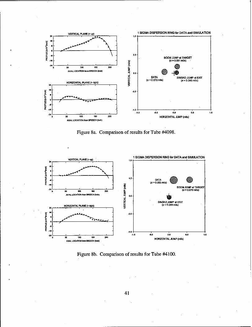
The results for each tube are presented as target impact plots of the firing data, projectile jump at exit from SIMBAD analysis, and impact location from BOOM projectile flight analysis in conjunction with SIMB AD exit conditions. The impact scale is angular with a range of 2.0 mils. The data are in the form of the three circles—one for the data, one for projectile jump at exit from SIMB AD, and one for target impact from BOOM flight simulation—the centers of which represent the location of the mean value for each result. The diameter of the circle represents the one-sigma circular dispersion band based upon a statistical analysis of the results. Presenting information in this manner lends itself to a concise and multifaceted comparison between the data and the results. In addition, the horizontal and vertical bore profile data and fit for each gun tube are shown and discussed in conjunction with the test and analysis results. Figures 8a through 8j contain this information.

Results for the five DIT indexed tubes are shown in Figures 8a through 8e. As noted previously, the vertical and horizontal shapes of the bore profile for these tubes are quite similar. In the vertical plane the muzzle points down with a fairly large bow, whereas the horizontal profile resembles a low amplitude sine wave, the muzzle of which sometimes points left and sometimes right. The calculated values for data and analysis shown on the right chart indicate the relative placement of the results with respect to the aim point (cross hairs). In four of the five cases for the DIT tubes, the results from the BOOM analysis show better correlation with data (at least in terms of mean values) than the SIMB AD exit conditions. The only exception is Tube #4098 for which the SIMBAD exit conditions are closer to actual impact data than those for BOOM. Circular dispersion calculations from SIMBAD range from 0.041 to 0.054 mil, whereas for BOOM they are 0.060 to 0.071 mil. The range for dispersion in the data is 0.070 to 0.199 mil. We must note that only three shots were fired in the test (in some cases only two were reported); therefore, the small sample size may not be representative of actual dispersion.

Results for the five STD indexed tubes are shown in Figures 8f through 8j. Since the top vertical centerline of these tubes is oriented such that the plane of maximum bending is vertical, the shapes for all five are very similar. The muzzle end points vertically upward with very little curvature in the horizontal plane. For all five cases, the mean values for the impact locations from the BOOM calculations are closer to the data than those for SIMBAD exit conditions. Circular dispersion calculations from SIMBAD range from 0.039 to 0.052 mil, whereas for BOOM they are 0.058 to 0.078 mil. The range for dispersion in the data is 0.028 to 0.256 mil.

An overall view of the analytical results for projectile jump is shown in Figure 9. The leftmost chart contains the mean jump values, as indicated from SIMBAD's calculation of the projectile's exit condition. The rightmost chart contains the mean values of the projectile's impact point from the BOOM analysis. The impact window is 2.0 mils by 2.0 mils. The SIMBAD results predict very little perturbation, since the mean jump values for all ten tubes are clustered around the cross hairs. However, the same cannot be said for the BOOM results. The

11

mean values for projectile impact from BOOM analysis are scattered about with none near the aim point. Recalling from Figure 1, the data values for impact locations are widely scattered as well.

A much better way of comparing the worth of these analytical results is to plot the differential jump mean values on an impact plot. Figure 10 contains this information. A differential jump in the mean is defined as the difference between the mean jump results from firing data and analysis. The leftmost chart contains these values using the SIMBAD analysis, whereas the rightmost chart contains the same using BOOM. If either model were a perfect predictor, then all differential values would be at the cross hairs. As expected, this is not the case. Since SIMBAD's raw jump values did not produce very much perturbation in the projectile's exit condition, the differential values from SIMBAD very nearly replicate the firing data. SIMBAD's differential values for nine of the ten tubes reside well above and to the right of the cross hairs, with the lone value just left of them. A one-sigma deviation ring plotted about the axis indicates the dispersion in these differential data. For the SIMBAD results, its value is 0.758 mil. On the rightmost chart, the differential jump mean values for the BOOM analysis are shown. The deviation ring using this analysis is 0.532 mil. There is a 30% improvement in simulation accuracy in predicting the mean jump values for a series of test shots over the SIMBAD results.

RECOMMENDATIONS AND CONCLUSIONS

The topics of gun dynamics modeling, bore profile estimates, projectile flight trajectory modeling, probabilistic analysis, and an integrated approach to estimating shot accuracy and dispersion have been cited in this report. This section contains discussions and analyses including the above topics, as well as conclusions based upon the findings from these analyses. The main points of the report will again be discussed in light of their relevance to the topics.

The first point concerns the relevance that bore profile and curvature have upon tube acceptability through the use of gun dynamics and projectile flight trajectory analysis. It is impossible to manufacture perfectly straight gun tubes due to their slenderness ratios and propensity to warp during manufacture. Current design specifications restrict the amount of profile deviation between measurement points and along the total length of the tube. The real culprit regarding dynamic excitation is not profile straightness, but rather local curvature. A gun tube may pass profile inspection, but it may possess high degrees of curvature along its entire length. A projectile forced to ride along this "bumpy path" will most certainly cause self-induced vibration and vibration to the tube as well.

Bore profile data for the ten tubes used in this test were presented, along with a method of determining a correct functional fit of the data points using the Chi-square statistic. Parameters of this method include both the number of inspection points and the accuracy of the inspection readings. By twice differentiating the profile fitting function, tube curvature is calculated. This tube parameter, which was different for each tube, proved to be critical in the overall analysis. The mean jump values for each gun tube were different, much like that of the data. The intent of

12

the DU test was to verify a tube indexing method that enhances accuracy. Results from studying a portion of the data indicate a definite migration of shot impact locations dependent upon the indexing method.

It may be concluded that a better method if specifying bore straightness, based upon local and overall curvature, needs to be developed. Possibly, the same type of algorithm to calculate profile and curvature used in this analysis may be incorporated in the inspection loop during tube manufacture. Curvature calculations may be reported, as well as profile data, with an acceptance criterion based upon curvature.

The second point involves the complexity of the models. The SIMBAD gun dynamics model is a finite element type analysis in which the structure is defined using beam finite elements. (Either the Euler-Bernoulli or Timoshenko formulation may be specified.) The calculation burden using this type of element is small compared to full three-dimensional elements. The degrees-of-freedom are on the order of hundreds instead of thousands for the three-dimensional models. The BOOM external flight model assumes that the projectile is a rigid body possessing only six degrees-of-freedom. Again, this minimizes the computational burden in predicting flight trajectories to the target. Although neither model is extremely complex, they seem to contain enough of the physics of the problem to be quite beneficial in predicting shotfall patterns and dispersions. Additionally, due to their computational speed, the time per run is small. Anyone versed in the use of these models may conduct studies involving 250 to 300 runs per day. This is beneficial when simulation is needed in a design environment to assess critical design parameters and determine sensitivities.

The third point involves the physics that was absent from these analyses. Since the testing was conducted on a round comprised of a long-rod penetrator, a flexible projectile was used in the SIMBAD model. The current version of SIMBAD does not support gravity on this type of round, moreover, the direction cosines of the penetrator at projectile exit are not calculated. The BOOM analysis uses direction cosines as initial conditions, and the off-diagonal terms seem to be quite important in predicting flight trajectories. For the analysis conducted herein, the direction cosine matrix was assumed to be a diagonal matrix of ones. The environmental conditions at the test site were unknown, therefore, standard atmosphere with no wind was used in the BOOM analysis. Sensitivities to these parameters were neither determined nor used in the dispersion studies. The stiffness response of the sabot's bore riders to the gun tube was based upon a static test conducted at the Army Research Lab. Benet Labs has funded a more detailed finite element method for this round using both pressure and acceleration as driving forces. This should improve the sabot/tube interface force/penetration values, the results of which may be applied to subsequent SIMBAD analyses.

The overall purpose of this study was to validate a coupled simulation package for predicting the impact location of test data from the Ml Al weapon. To the authors' knowledge, this has been the first system analysis of coupled gun dynamics and projectile flight simulation codes. The integration of both was not trivial due to the idiosyncrasies of each, namely, their dissimilar coordinate systems. At first the lack of critical data was thought to be a shortcoming,

13

however, after much "legwork" and shrewd engineering analysis, this proved not to be the case. These data were determined and applied to the modeling effort, the results of which showed very good correlation with field-generated test results. This proves that simulation for accuracy from breech to target is achievable using moderately complex models in the hands of expert weapon analysts. It is our recommendation that further study, including more rounds and more gun tubes, is warranted with the intent of gaining improved accuracy (albeit slight) across the full family of rounds for Ml A2 tanks or any other large caliber weapon in the U.S. Army's inventory.

14

REFERENCES

1. Schmidt, E., "A Method for Indexing Tank Cannon," BRL IMP 912, Ballistic Research Laboratory, Aberdeen Proving Ground, MD, 1988.

2. Webb, D., Thomas L, and Carter, R., "Ml Al Tank DIT Experiment: Analysis and Results," BRL-MR3962, U.S. Army Lab Command, Aberdeen Proving Ground, MD, 1992.

3. Gast, R., "Curvature-Induced Motion of 60-mm Guns, Phase I: Test Results," ARDEC Technical Report ARCCB-TR-92048, Benet Laboratories, Watervliet, NY, November 1992.

4. Gast, R., "Curvature-Induced Motions of 60-mm Guns, Phase II: "Modelling," ARDEC Technical Report ARCCB-TR-94002, Benet Laboratories, Watervliet, NY, January 1994.

5. Simkins, T., "Transverse Response of Gun Tubes to Curvature-Induced Load Functions," Proceedings of the Second U.S. Army Symposium on Gun Dynamics, ARLCB-SP-78013, Benet Laboratories, Watervliet, NY, 1978, pp. 1-66 to 1-77.

6. Börse, G., Fortran 77 and Numerical Methods for Engineers, PWS-Kent Publishing Company, Boston, MA, 1985, pp. 469-471.

7. Lyon D., "Radial Stiffness Measurements of 120mm Tank Projectiles," ARL-TR-392, Army Research Laboratory, Aberdeen Proving Ground, MD, 1994.

8. Wilkerson, S., Army Research Laboratory, Aberdeen Proving Ground, MD, and Gast, R., Benet Laboratories, Watervliet, NY, private conversation, 1995.

15

1.5 4

1.0

1 a. 3

I-

UJ >

0.5

0.0 -

-0.5 -1.0

CO! MEAN VALUES for DATA

STD TUBES ▲ A A

DIT TUBES

-0.5 0.0 0.5

HORIZONTAL JUMP (mils)

1.0

Figure 1. Average centers of impact for select tubes in DIT test.

16

MEASUREMENT ERROR FUNCTIONAL FIT IS OVER CONSTRAINED (PASSES THROUGH EACH DATA POINT)

MEASUREMENT ERROR

DATA POINTS

FUNCTIONAL FIT IS UNDER CONSTRAINED (MISSES MOST ERROR BARS)

MEASUREMENT ERROR

FUNCTIONAL FIT IS APPROPRIATELY CONSTRAINED (PASSES THROUGH ERROR BARS BUT NOT THROUGH EACH POINT)

DATA POINTS

Figure 2. Curve fitting process for data processing errors in measurement.

17

X2 » (N - g) - poor fit = ~ (N - g) - adequate fit

« (iV - g) - constrained fit

N = Number of data points g = Number of fit parameters

Figure 3. Chi-square method for fitting data with measurement error.

18

24

.-. 16 - ü c

CT 8 o ▼— .X, 0 UJ —1

-8 DU Q. -16

-24 50 100 150

AXIAL LOCATION from BREECH (inch)

200

50 100 150


200

Figure 4a. Vertical profile and curvature for Tube #4098.

19

24

~ 16 c

n 8 O IT" ,X, 0 tu _l u. -8 o a: a. -16

-24 50 100 150

AXIAL LOCATION from BREECH Onch)

200

50 100 150


200

Figure 4b. Vertical profile and curvature for Tube #4100.

20

24

35T 16 u c

m^~ 8 Ö

£ 0 UJ

(3rt ORDER FIT)

O en °- -16

-24

8 -

• _• •

50 100 150


200

50 100 150


200

Figure 4c. Vertical profile and curvature for Tube #4102.

21

50 100 150


200

-40 50 100 150


200

Figure 4d. Vertical profile and curvature for Tube #4104.

22

o c

o 3<,

UJ _j u_ O a: Q.

50 100 150


200

50 100 150


200

Figure 4e. Vertical profile and curvature for Tube #4106.

23

50 100 v 150


200

50 100 150


200

Figure 4f. Vertical profile and curvature for Tube #4988.

24

50 100 150


200

u c

CO

Ö

HI a:

I 50 100 150


Figure 4g. Vertical profile and curvature for Tube #4990.

25

24

.-. 16 - ü c

cT" 8 Ö T- g.

0 w —1 IX. -R O Q: a. -16

-24 50 100 150


200

50 100 150


200

Figure 4h. Vertical profile and curvature for Tube #4992.

26

u c

o .X,

uu _J u_ O en Q.

50 100 150

AXIAL LOCATION from BREECH önch)

200

-40 50 100 150


200

Figure 4i. Vertical profile and curvature for Tube #4994.

27

50 100 150


200

u c ^ 20

w a:

I Ü

-40 50 100 150


200

Figure 4j. Vertical profile and curvature for Tube #4996.

28

50 100 • 150


200

-40 50 100 150


200

Figure 5a. Horizontal profile and curvature for Tube #4098.

29

ü c

o 5, lil _J u. O 01 0_

50 100 150


200

40

u c ^ 20

UJ a:

I O

-20 -

-40

t I I I

50 100 150


200

Figure 5b. Horizontal profile and curvature for Tube #4100.

30

50 100 150

AXIAL LOCATION from BREECH Qnch)

200

o c J^ 20 -

a:

I ü

-40 50 100 150


200

Figure 5c. Horizontal profile and curvature for Tube #4102.

31

24

2? 16 o c

fc> .X,

Ui -J u_ o cr: a.

- (2nd ORDER FIT)

8 -

0

-8

-16

-24

-=*=w-»-*=*= -• •■

• • • "■*■*»« •

50 100 150


200

50 100 150


200

Figure 5d. Horizontal profile and curvature for Tube #4104,

32

50 100 150


50 100 150


200

Figure 5e. Horizontal profile and curvature for Tube #4106.

33

50 100 150


200

JC Ü c ^ 20

a:

I Ü

50 100 150


200

Figure 5f. Horizontal profile and curvature for Tube #4988.

34

24

S 16 u _c

m~* 8 Ö

I 0 1X1

-8 - O a: °- -16

-24

I I

(5th ORDER FIT)

I I

-

»• -

►—*-• • • »- • »-*-

I I i i

-

50 100 150


200

50 100 150


200

Figure 5g. Horizontal profile and curvature for Tube #4990.

35

o 5, w _J U_ O a: a.

50 100 ' 150


200

-40 50 100 150


200

Figure 5h. Horizontal profile and curvature for Tube #4992.

36

24

E- 16 o

#c n~* 8 Ö

I 0 UJ

u. O Q.

(3rt ORDER FIT)

-8

-16

• • »-JL.

• »^ -*•••-»

-24 50 100 150


200

50 100 150


200

Figure 5i. Horizontal profile and curvature for Tube #4994.

37

50 100 150


200

O c

(D

Ö

HI a:

I Ü

50 100 150


200

Figure 5j. Horizontal profile and curvature for Tube #4996.

38

120mm GENERIC KINETIC ENERGY ROUND

GUN TUBE

FINS SABOT (3 petals)

PENETRATOR

REAR BORE RIDER FRONT BORE RIDER

Figure 6. Schematic of kinetic energy round in gun bore.

39

120mm M256 CANNON and MOUNT

BREECH (attached to piston) THRUST NUT

(threaded to bearing)

BEARING

GUN TUBE

RECUPERATOR SPRING

KING NUT (threaded to tube)

ADAPTOR

For Clarity the radial scale is exaggerated and numerous features are not shown.

Figure 7. Schematic of Ml Al gun mount and cannon.

40

VERTICAL PLANE (+up) 1 SIGMA DISPERSION RING for DATA and SIMULATION

» 100 150 200

AXIAL LOCATION Horn BREECH (Inch)

HORIZONTAL PLANE (+ right)

50 100 150

AXIAL LOCATION tram BREECH (Inch)

s

BOOM JUMP at TARGET (o = 0.061 mils)

DATA (o = 0.070 mils)

SIMBAD JUMP at EXIT (0 = 0.046 mils)

•0.5 0.0 0.5


Figure 8a. Comparison of results for Tube #4098.

— IS

i • £ o

•5 #■ . o

£ o a £ •«

VERTICAL PLANE (+up)

so 100 ISO

AXIAL LOCATION «Torn BREECH (Inch)


y" »»-«<« . .-

SO 100 150 200

AXIAL LOCATION «ram BREECH (Inch)

1 SIGMA DISPERSION RING for DATA and SIMULATION

s


BOOM JUMP at TARGET (0 = 0.070 mils)


4.5 0.0 0.5


Figure 8b. Comparison of results for Tube #4100.

41

f- «

24

I'6 ?■ » o

I o

tc «• -16 -

-24


-r"

50 100 150 . 200

AXIAL LOCATION from BREECH (Inch)

HORIZONTAL PLANE (+ light)

50 100 150 200



BOOM JUMP at TARGET (0 = 0.069 nils)

DATA (a = 0.081 mils)

SIMBAD JUMP at EXIT (o = 0.054 mils)

-0.5 o.o 0.5


Figure 8c. Comparison of results for Tube #4102.

— 16 -

•r » -

6 ■• DC

■■ -16

VERTICAL PLANE (»up)

50 100 150 200



50 100 150 200



3! o

DATA (0 = 0.134 mils)

BOOM JUMP at TARGET

SIMBAD JUMP at EXIT ' (° = 0060 mte> (0 = 0.042 mils)

-0.5 o.o 0.5


Figure 8d. Comparison of results for tube #4104.

42

VERTICAL PLANE (tup) 1 SIGMA DISPERSION RING for DATA and SIMULATION

f "

3

AXIAL LOCATION ton BREECH (to*)

HORIZONTAL PLANE (♦ right)

S => -9

5! Ü p

DATA 1|| (0 = 0.199 mils) ^if

• BOOM JUMP at TARGET

(o * 0.067 mils)

^n~~

SIMBAD JUMP at EXrr (0 = 0.041 mils)

0 50 100 150 200

AXIAL LOCATION tan BREECH (hdi)

0.0 0.5


Figure 8e. Comparison of results for Tube #4106.


f,6 ?■ « o

)

-

111

i * OS

°- -16

^v» /


*

i o ui

s •• a: ■>- -16

-2«

50 100 150 200



SO 100 150 200

AXIAL LOCATION fiom BREECH (Inch)

s




-0.5 0.0 0.5


Figure 8f. Comparison of results for Tube #4988.

43

£ 8


50 100 ISO 200



50 100 150 200



E 0.5

K 0.0


BOOM JUMP at TARGET (a = 0.078 mils)

» + SIMBAD JUMP at EXIT

(0 = 0.052 mils)

•0.5 0.0 0.5


Figure 8g. Comparison of results for Tube #4990.


£ o ui

§ -« °- -16

£ 0

SO 100 150 200


HORIZONTAL PLANE {+ right)

50 100 150 200



1 0.5

DATA (0=0.125 mils)


SIMBAD JUMP at EXIT (0=0.046 mils)


Figure 8h. Comparison of results for Tube #4992.

44

VERTICAL PLANE (+up) 1 SIGMA DISPERSION RING for DATA and SIMULATION

SO 100 150

AXIAL LOCATION train BREECH (Inch)

HORIZONTAL PLANE {+ right)

50 10O 150 200


or s

/B. DATA

(0=0.256 mils)

BOOM JUMP at TARGET (0=0.062 mils)

SIM BAD JUMP at EXIT (0 = 0.039 mils)

■0.5 0.0 0.5


Figure 8i. Comparison of results for Tube #4994.

6


50 100 150 200


24

I " o


«■•*•' *-»■--—. £ 0 UJ

1 - °- -18 -

■ i i i

50 100 ISO 200


1 SIGMA DISPERSION RING tor DATA and SIMULATION

0. £ =>



SIMBAD JUMP at EXrT (o=0.046 mils)

•0.5 , o.o 0.5


Figure 8j. Comparison of results for Tube 4996.

45

COI MEAN VALUES for SIMBAD SHOT DOT COI MEAN VALUES for BOOM TARGET IMPACT

-1.0 -0.5 0.0 0.5


-1.0 -0.5 0.0 0.5


Figure 9. Comparison of calculated impact mean value results of both models for all tubes.

DIFFERENTIAL COI MEAN VALUES from SIMBAD to DATA DIFFERENTIAL COI MEAN VALUES from BOOM to DATA

1J).

• •

as- • v 0.758 mils

0.0- { •

-0.5- /

■as o.o os


•OS 0.0 OS 1.0

HORIZONTAL JUMP (m»s)

Figure 10. Comparison of differential results for impact mean values for all tubes.

46

TECHNICAL REPORT INTERNAL DISTRIBUTION LIST

NO. OF COPIES

TECHNICAL LIBRARY ATTN: AMSTA-AR-CCB-0

TECHNICAL PUBLICATIONS & EDITING SECTION ATTN: AMSTA-AR-CCB-0

OPERATIONS DIRECTORATE ATTN: SIOWV-ODP-P

DIRECTOR, PROCUREMENT & CONTRACTING DIRECTORATE ATTN: SIOWV-PP

DIRECTOR, PRODUCT ASSURANCE & TEST DIRECTORATE ATTN: SIOWV-QA

NOTE: PLEASE NOTIFY DIRECTOR, BENET LABORATORIES, ATTN: AMSTA-AR-CCB-0 OF ADDRESS CHANGES.

TECHNICAL REPORT EXTERNAL DISTRIBUTION LIST

DEFENSE TECHNICAL INFO CENTER ATTN: DTIC-OCA (ACQUISITIONS) 8725 JOHN J. KINGMAN ROAD STE0944 FT. BELVOIR, VA 22060-6218

COMMANDER U.S. ARMY ARDEC ATTN: AMSTA-AR-WEE, BLDG. 3022

AMSTA-AR-AET-O, BLDG. 183 AMSTA-AR-FSA, BLDG. 61 AMSTA-AR-FSX AMSTA-AR-FSA-M, BLDG. 61 SO AMSTA-AR-WEL-TL, BLDG. 59

PICATINNY ARSENAL, NJ 07806-5000

DIRECTOR U.S. ARMY RESEARCH LABORATORY ATTN: AMSRL-DD-T, BLDG. 305 ABERDEEN PROVING GROUND, MD

21005-5066

DIRECTOR U.S. ARMY RESEARCH LABORATORY ATTN: AMSRL-WM-MB (DR. B. BURNS) ABERDEEN PROVING GROUND, MD

21005-5066

NO. OF NO. OF COPIES

COMMANDER

COPIES

2 ROCK ISLAND ARSENAL ATTN: SIORI-SEM-L 1 ROCK ISLAND, EL 61299-5001

COMMANDER U.S. ARMY TANK-AUTMV R&D COMMAND ATTN: AMSTA-DDL (TECH LIBRARY) 1 WARREN, MI 48397-5000

COMMANDER U.S. MILITARY ACADEMY ATTN: DEPT OF CIVIL & MECH ENGR 1 WEST POINT, NY 10966-1792

U.S. ARMY AVIATION AND MISSILE COM REDSTONE SCIENTIFIC INFO CENTER 2 ATTN: AMSAM-RD-OB-R (DOCUMENTS) REDSTONE ARSENAL, AL 35898-5000

COMMANDER U.S. ARMY FOREIGN SCI & TECH CENTER ATTN: DRXST-SD 1 220 7TH STREET, N.E. CHARLOTTESVILLE, VA 22901

COMMANDER U.S. ARMY RESEARCH OFFICE ATTN: TECHNICAL LIBRARIAN P.O. BOX 12211 4300 S. MIAMI BOULEVARD RESEARCH TRIANGLE PARK, NC 27709-2211

NOTE: PLEASE NOTIFY COMMANDER, ARMAMENT RESEARCH, DEVELOPMENT, AND ENGINEERING CENTER, BENET LABORATORIES, CCAC, U.S. ARMY TANK-AUTOMOTIVE AND ARMAMENTS COMMAND,

AMSTA-AR-CCB-O, WATERVLET, NY 12189-4050 OF ADDRESS CHANGES.

Documents

SIMULATION OF SHOT IMPACTS FOR THE M1A1 TANK … · SIMULATION OF SHOT IMPACTS FOR THE ... all are used for design evaluation. ... DYNAMIC INDEXING OF GUN TUBES AND TEST RESULTS The