SIMULATION OF ORTHOGONAL METAL CUTTING BY FINITE ELEMENT ANALYSIS

A THESIS SUBMITTED TO THE GRADUATE SCHOOL OF NATURAL AND APPLIED SCIENCES

OF THE MIDDLE EAST TECHNICAL UNIVERSITY

BY

HALİL BİL

IN PARTIAL FULFILLMENT OF THE REQUIREMENTS FOR THE DEGREE OF

MASTER OF SCIENCE

IN

THE DEPARTMENT OF MECHANICAL ENGINEERING

AUGUST 2003

Approval of the Graduate School of Natural and Applied Sciences.

Prof. Dr. Canan ÖZGEN Director

I certify that this thesis satisfies all requirements as a thesis for the degree of Master of Science.

Prof. Dr. Kemal İDER Head of Department

This is certify that we have read this thesis and that in our opinion it is fully adequate, in scope and quality, as a thesis for the degree of Master of Science.

Prof. Dr. A. Erman Tekkaya Prof. Dr. S. Engin Kılıç Co-Supervisor Supervisor

Examining Committee Members: Prof. Dr. Alp ESİN (Chairperson)

Prof. Dr. S. Engin KILIÇ (Supervisor)

Prof. Dr. A. Erman TEKKAYA (Co-Supervisor)

Asst. Dr. Serkan DAĞ

Prof. Dr. Turgut TOKDEMİR

ABSTRACT

SIMULATION OF ORTHOGONAL METAL CUTTING BY FINITE

ELEMENT ANALYSIS

Halil BİL

M.Sc., Department of Mechanical Engineering

Supervisor: Prof. Dr. S. Engin KILIÇ

Co-Supervisor: Prof. Dr. A. Erman TEKKAYA

August 2003, 115 pages

The aim of this thesis is to compare various simulation models of orthogonal

cutting process with each other as well as with various experiments. The effects

of several process parameters, such as friction and separation criterion, on the

results are analyzed. As simulation tool, commercial implicit finite element codes

MSC.Marc, Deform2D and the explicit code Thirdwave AdvantEdge are used.

Separation of chip from the workpiece is achieved either only with continuous

remeshing or by erasing elements according to the damage accumulated. From

the results cutting and thrust forces, shear angle, chip thickness and contact length

between the chip and the rake face of the tool can be estimated. For verification

of results several cutting experiments are performed at different cutting

conditions, such as rake angle and feed rate. Results show that commercial codes

are able to simulate orthogonal cutting operations within reasonable limits.

Friction is found to be the most critical parameter in the simulation, since good

agreement can be achieved for individual process variables by tuning it.

Therefore, simulation results must be assessed with all process variables and

friction parameter should be tuned according to the shear angle results.

iii

Plain damage model seems not appropriate for separation purposes of machining

simulations. On the other hand, although remeshing gives good results, it leads to

the misconception of crack generation at the tip of the tool. Therefore, a new

separation criterion is necessary to achieve both good physical modeling and

prediction of process variables.

Keywords: Finite Element Method, Orthogonal Metal Cutting, Remeshing,

Damage, Friction.

iv

ÖZ

DİK KESME İŞLEMLERİNİN SONLU ELEMAN ANALİZİ İLE

SİMULASYONU

Halil BİL

Yüksek Lisans, Makine Mühendisliği Bölümü

Tez Yöneticisi: Prof. Dr. S. Engin KILIÇ

Yardımcı Tez Yöneticisi: Prof. Dr. A. Erman TEKKAYA

Ağustos 2003, 115 sayfa

Bu tezin amacı, dik kesme işlemleri için geliştirilmiş çeşitli sonlu eleman

modellerinin birbirleriyle ve deneyler ile karşılaştırılmasıdır. Sürtünme koşulları

ve ayrılma kriterleri gibi parametrelerin sonuçlar üzerindeki etkisi incelenmiştir.

Simülasyon aracı olarak, kapalı kodlar olan MSC.Marc ve Deform2D ile açık bir

kod olan Thirdwave AdvantEdge kullanılmıştır. Talaşın iş parçasından ayrılması,

sürekli yeni ağ tanımlanması veya elemanların toplam hasara göre silinmesi ile

elde edilmiştir. Sonuçlardan, kesme ve ilerleme kuvvetleri, kayma açısı, talaş

kalınlığı ve kalem ile talaş arasındaki temas uzunluğu tahmin edilebilmektedir.

Sonuçların doğrulanması için değişik kesme koşullarında (kesme açısı ve

ilerleme hızı) deneyler yapılmıştır. Sonuçlar, ticari yazılımlarının dik kesme

işlemlerini kabul edilebilir sınırlar içerisinde simüle edebileceğini göstermiştir.

Sürtünme koşullarının simülasyonu etkileyen en önemli parametre olduğu

bulunmuştur. Çünkü, bu parametrenin ayarlanması ile her işlem değişkeni için

ayrı ayrı iyi sonuçlar elde edilebilmektedir. Dolayısıyla, simülasyon sonuçları

v

bütün işlem değişkenleri ile değerlendirilmelidir. Ayrıca, sürtünme koşulları

kayma açısına göre ayarlanmalıdır.

Hasar modellerinin talaşın iş parçasından ayrılması amacı ile kullanılması uygun

değil gibi görünmektedir. Yeni ağ tanımlanması ise iyi sonuçlar vermesine

rağmen, iş parçası malzemesinde çatlak oluşması gibi bir kavram hatasına yol

açmaktadır. Dolayısıyla, hem iyi bir fiziksel modelleme yapılması hem de işlem

değişkenlerinin doğru tahmin edilebilmesi için yeni bir ayrılma kriterine ihtiyaç

vardır.

Keywords: Finite Element Method, Orthogonal Metal Cutting, Remeshing,

Damage, Friction.

vi

To my family and Dilek Başaran.

vii

ACKNOWLEDGEMENTS

I would like to express my appreciation to my supervisor Prof. Dr. S. Engin

KILIÇ and my co-supervisor Prof. Dr. A. Erman TEKKAYA for their help and

inspiration through out my thesis.

I am also grateful to the Femlab members: Kurşad Kayaturk, Ahmet Kurt, Özgür

Koçak, Bahadır Koçaker, Muhsin Öcal and Mete Egemen for making the

working days and nights in the laboratory a joy.

The support of Mechanical Engineering Department and Graduate School of

Natural and Applied Sciences is also very much appreciated. I am also thankful to

Ercenk Aktay from Figes Company, who made Thirdwave AdvantEdge available

to use.

Lastly, I would like to express my deepest gratitude and respect to my family

who made all the things possible. Their support and patience are just making me

feel better.

viii

TABLE OF CONTENTS

Abstract ………………………………………………………………………... iii

Öz ……………………………………………………………………………… v

Dedication ……………………………………………………………………… vii

Acknowledgements ……………………………………………………………. viii

Table of Contents ……………………………………………………………… ix

List of Tables ………………………………………………………………….. xii

List of Figures ………………………………………………………………….. xiii

List of Symbols and Abbreviations ……………………………………………. xviii

CHAPTERS

1 INTRODUCTION ……………………………………………………. 1

1.1 Introduction ……………………………………………………………. 1

1.2 Aim and Scope of the Study ………………………………………….. 4

1.3 Finite Element Models and Experiments ……………………………… 5

1.4 Content of this Study ………………………………………………….. 6

2 LITERATURE SURVEY ……………………………………………. 7

2.1 Introduction ……………………………………………………………. 7

2.2 Chip Formation and Nomenclature ……………………………………. 7

2.3 Shear Zone Models ……………………………………………………. 15

2.4 Shear Angle Relationships ……………………………………………. 16

2.4.1 Merchant's Relationship ……………………………………………… 17

ix

2.4.2 Lee and Shaffer's Relationship ………………………………………......18

2.4.3 Oxley's Relationship …………………………………………………….18

2.4.4 Other Relationships ………………………………………………………18

2.5 Friction on the Rake Face of a Cutting Tool …………………………….19

2.6 The Shear Stress in Shear Zone During Metal Cutting …………………..21

2.7 Numerical Approach …………………………………………………….24

2.7.1 Steady State Solutions …………………………………………………..24

2.7.2 Solutions for Continuous Chip Formation ………………………………29

2.7.3 Solutions for Transient Chip Formation ………………………………...29

2.7.4 Solutions for Transient and Continuous Chip Formation ………………31

2.8 Conclusion ………………………………………………………………38

3 EXPERIMENTAL WORK …………………………………………….39

3.1 Introduction ………………………………………………………………39

3.2 Orthogonal Cutting ………………………………………………………40

3.3 Workpiece Material ………………………………………………………41

3.4 Test Setup ………………………………………………………………...42

3.5 Cutting Experiments Performed in This Work …………………………..49

3.6 Compression Test ………………………………………………………...50

4 NUMERICAL MODEL OF ORTHOGONAL METAL CUTTING.. 53

4.1 Introduction ………………………………………………………………53

4.2 Finite Element Models …………………………………………………..54

4.2.1 Finite Element Model with MSC.Marc …………………………………..54

4.2.2 Finite Element Model with Deform2D …………………………………..63

4.2.3 Finite Element Model with Thirdwave AdvantEdge …………………….66

4.3 Comparison of Finite Element Models …………………………………..71

x

5 RESULTS AND COMPARISON …………………………………….72

5.1 Introduction ………………………………………………………………72

5.2 Comparison with Analytical Solutions …………………………………..75

5.3 Comparison of Chip Geometry …………………………………………..77

5.4 Comparison of Cutting Forces …………………………………………..92

5.5 Comparison of Thrust Forces …………………………………………….96

5.6 Comparison of Simulation with the Experimental Results from

Literature ………………………………………………………………...100

6 DISCUSSION AND CONCLUSION …………………………………..104

6.1 Introduction ………………………………………………………………104

6.2 Effect of Friction ………………………………………………………...105

6.3 Effect of Material Modeling …………………………………………….106

6.4 Effect of Chip Separation Criterion …………………………………….107

6.5 Computational Aspects …………………………………………………..108

6.6 Conclusion ………………………………………………………………109

6.7 Recommendation for Future Work …………………………………….. 110

References ………………………………………………………………………112

xi

LIST OF TABLES

3.1 Chemical composition of C15 steel in weight percent. ………………...41

3.2 Mechanical and thermal properties of the workpiece

material, C15 steel ……………………………………………………....42

3.3 Specifications of the Topcon Universal Measuring Microscope. ………47

3.4 Cutting conditions at which experiments were performed. …………….49

4.1 Comparison of three commercial codes. ………………………………71

5.1 Simulations were done under four different cutting conditions. ………72

5.2 Experimental results of chip geometry parameters …………………….78

5.3 Chip geometry results with MSC.Marc. ………………………………78

5.4 Chip geometry results from Deform2D. ………………………………81

5.5 Chip geometry results from Thirdwave AdvantEdge. ………………...84

5.6 Cutting conditions for the chip geometry verification. ………………...89

5.7 Experimentally measured cutting force results.………………………...92

5.8 Predicted cutting force results from MSC.Marc. ………………………92

5.9 Predicted cutting force results from DEFORM2D. …………………….93

5.10 Predicted cutting force results from Thirdwave AdvantEdge. ………...94

5.11 Experimentally measured thrust force results. ………………………...96

5.12 Predicted thrust force results estimated by MSC.Marc.………………...97

5.13 Predicted thrust force results from DEFORM2D.………………………98

5.14 Predicted thrust force results from Thirdwave AdvantEdge. …………..99

5.15 Experimental and Simulation results of Movahhedy and Altintas. …….101

5.16 Comparison with literature (m=0.1). …………………………………..101

5.17 Comparison with literature (m=0.7). …………………………………..101

xii

LIST OF FIGURES

2.1 Orthogonal and Oblique Cutting………………………………………... 8

2.2 Chip samples produced by quick stop techniques………………………. 9

2.3 Some of the variables in orthogonal cutting…………………………….. 10

2.4 Assumed shape of deformation zone in cutting………………………..... 11

2.5 A photomicrograph of orthogonal cutting operation

where thin shear plane is approached…………………………………… 12

2.6 An illustration of the mechanism of discontinuous chip formation…….. 12

2.7 Idealized picture of built-up edge (B.U.E) formation…………………… 13

2.8 Typical shape of the stress-strain relationship for

a metal under the action of a tensile stress……………………………… 14

2.9 Shear zone types………………………………………………………… 16

2.10 Variables used in shear angle relationships……………………………... 17

2.11 Dependence of friction force to the normal force……………………….. 20

2.12 Frictional shear stress distribution on rake face of the tool……………... 21

2.13 Pre-Flow region…………………………………………………………. 22

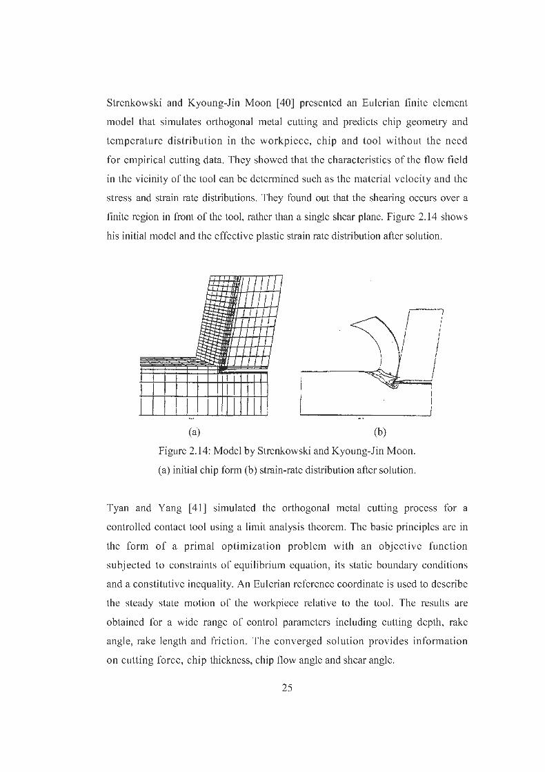
2.14 Model by Strenkowski and Kyoung-Jin Moon………………………….. 25

2.15 Model by Stevenson, Wright and Chow………………………………… 27

2.16 Initial and deformed of the model by Arola and Ramulu……………….. 30

2.17 Model developed Carroll and Strenkowski……………………………... 31

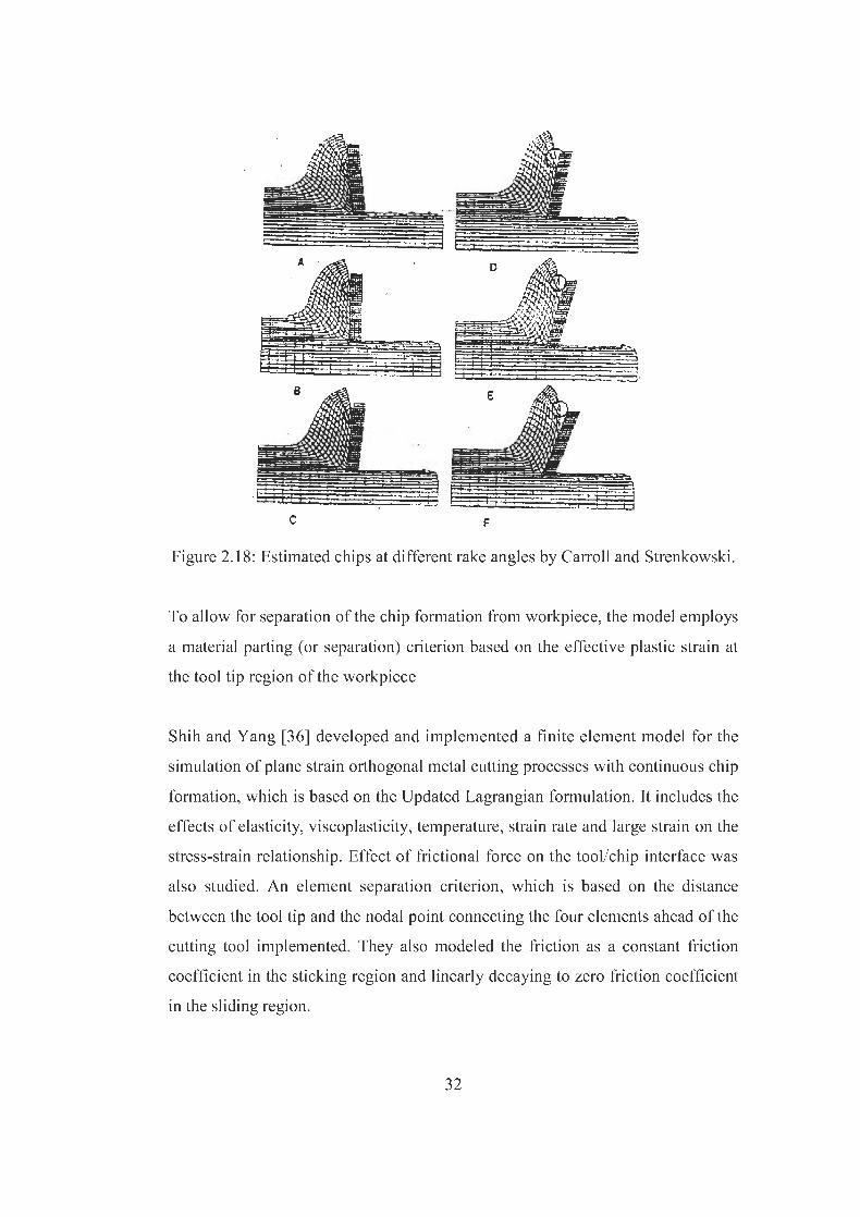
2.18 Estimated chips at different rake angles by Carroll and Strenkowski…... 32

2.19 The initial finite element mesh, configuration of the cutting

tool and dimensions of the elements developed by Shih………………... 34

xiii

2.20 Remeshing module used by Ceretti, Lucchi and Altan…………………. 35

2.21 Oxley’s theory and its simplified flow chart……………………………. 36

2.22 Results of the work done by Borouchaki, Cherouat,

Laug and Saanouni……………………………………………………… 37

3.1 Schematic representation of orthogonal cutting and

velocity diagram………………………………………………………… 40

3.2 Orthogonal turning operation on a lathe………………………………… 41

3.3 Test Setup……………………………………………………………….. 42

3.4 Lathe tool dynamometer setup………………………………………….. 43

3.5 Analog display of the dynamometer……………………………………. 44

3.6 Calibration of the dynamometer………………………………………… 45

3.7 Calibration curve for cutting force……………………………………… 45

3.8 Calibration curve for thrust force……………………………………….. 46

3.9 Contact length on the rake face of the tool……………………………… 47

3.10 Microscope by which the thicknesses of chips were measured…………. 48

3.11 A sample microscope view while measuring thickness………………… 48

3.12 Comparison of experimental and simulated

compressed specimens…………………………………………………... 51

3.13 Comparison of punch displacement – punch force diagram……………. 52

4.1 Finite element model of MSC.Marc…………………………………….. 54

4.2 Quadrilateral element…………………………………………………… 55

4.3 Distribution of generated heat due to friction…………………………… 57

4.4 Workpiece flow curve for strain-rate of 40 (s-1)………………………... 58

4.5 Workpiece flow curve for strain-rate of 8 (s-1)…………………………. 59

4.6 Workpiece flow curve for strain-rate of 1.6 (s-1)……………………….. 59

4.7 Effect of strain-rate on the flow curves…………………………………. 60

4.8 Step function frictional stress and approximation by Equation 4.5……... 61

xiv

4.9 Separation of chip from the workpiece by continuous remeshing……… 63

4.10 Finite element model of Deform2D…………………………………….. 64

4.11 Element erase due to damage via remeshing in Deform2D...................... 65

4.12 Finite element model of Third Wave Systems AdvantEdge……………. 67

4.13 Six-noded triangular element……………………………………………. 69

5.1 A typical diagram of cutting force versus increment number…………... 73

5.2 Effect of contact penetration value……………………………………… 74

5.3 Effect of penetration check method on the results………………………. 74

5.4 Rake, Shear and Friction angle for an orthogonal cut…………………... 76

5.5 Allowable slip-line model solutions for rake angle of 20°……………… 76

5.6 Allowable slip-line model solutions for rake angle of 25°……………… 77

5.7 Shear angle can be found from strain-rate distribution…………………. 79

5.8 Effect of friction factor on the chip thickness results obtained

by MSC.Marc…………………………………………………………… 80

5.9 Effect of friction factor on the shear angles obtained by

MSC.Marc calculated from chip thickness results.……………………... 80

5.10 Effect of friction factor on the contact length results

by MSC.Marc…………………………………………………………… 81

5.11 Effect of friction factor on the chip thickness results

by Deform2D……………………………………………………………. 82

5.12 Effect of friction factor on the shear angles obtained by

Deform2D calculated from chip thickness results.…………………….... 83

5.13 Effect of friction factor on the contact length results by Deform2D……. 83

5.14 Effect of friction factor on the chip thickness results by Thirdwave

AdvantEdge………………………………………………………………85

5.15 Effect of friction factor on the shear angles obtained by Thirdwave

AdvantEdge calculated from chip thickness results…………………….. 85

xv

5.16 Effect of friction factor on the contact length

by Thirdwave AdvantEdge……………………………………………… 86

5.17 Comparison of chip thickness results from three

codes with experiments………………………………………………….. 87

5.18 Shear angles obtained by three codes from chip thickness estimation...... 88

5.19 Comparison of contact length results from three

codes with experiments………………………………………………….. 90

5.20 Simulated chip geometries from three commercial

codes at 20° rake angle………………………………………………….. 91

5.21 Simulated chip geometries with three commercial

codes at 25° rake angle………………………………………………….. 93

5.22 Effect of Friction on the cutting force results of MSC.Marc……………. 94

5.23 Effect of friction on the cutting force results of Deform2D…………….. 95

5.24 Effect of friction on the cutting force results of

Thirdwave AdvantEdge…………………………………………………. 95

5.25 Comparison of cutting forces estimated by

three codes and experiments…………………………………………….. 96

5.26 Forces acting on the tool……………………………………………….... 97

5.27 Effect of friction factor on the thrust force prediction of MSC.Marc….... 98

5.28 Effect of friction factor on the thrust force prediction

of Deform2D…………………………………………………………….. 99

5.29 Effect of friction factor on the thrust force

by Thirdwave AdvantEdge……………………………………………… 100

5.30 Comparison of thrust forces estimated by three

codes and experiments…………………………………………………... 102

5.31 Comparison of cutting and thrust forces obtained

by MSC.Marc with experiment from literature…………………………. 102

xvi

5.32 Comparison of shear angle obtained by MSC.Marc

with experiment from literature…………………………………………. 103

5.33 Comparison of contact length obtained by MSC.Marc

with experiment from literature…………………………………………. 103

5.34 Comparison of contact length estimated by MSC.Marc

with experiment from literature………………………………………….

6.1 Crack generated by remeshing…………………………………………... 108

xvii

LIST OF SYMBOLS AND ABBREVIATIONS

θ Angle of Obliqueness

ac Uncut Chip Thickness

a0 Chip Thickness

γ Rake Angle

φ Shear Angle

α Clearance Angle

V Relative Velocity Between Tool and Workpiece

Vc Cutting Speed

B.U.E. Built-Up Edge

β Friction Angle

Ff Frictional Force

Fn Normal Force

F Equivalent Force

µ Friction Coefficient

h1 Length of Sticking Region

h2 Length of Sliding Region

δ ratio of the plastic zone thickness to the cut chip thickness

lc Contact Length

Vs Shearing Speed at Shear Zone

q Heat

h Convection Heat Transfer Coefficient

Tw Workpiece Surface Temperature

T0 Ambient Temperature

Ffr Frictioanl Force

vr Relative Sliding Velocity Between Tool and Chip

xviii

M Mechanical Equivalent of Heat

R Rate of Specific Volumetric Flux

f Fraction of Plastic Work Converted into Heat or Feed Rate

Wp Rate of Plastic Work

ρ Density

ε Strain-Rate

m Friction Factor

ky Shear Yield Stress

t Tangential Vector

σ Equivalent Stress

C Critical Damage Value

Qchip Heat Given to Chip

Qtool Heat Given to Tool

Qfriction Heat Genetared due to Friction

σf Flow Stress

εp Accumulated Plastic Strain

0pε Reference Plastic Strain-Rate

m1 Low Strain-Rate Sensitivity Exponent

m2 High Strain-Rate Sensitivity Exponent

tε Treshold Strain Rate

T Current Temperature

σ0 Initial Yield Stress

T0 Reference Temperature

0pε Reference Plastic Strain

T(T) Thermal Softening Factor

rc Chip Thickness Ratio

dc Depth of Cut

Fc Cutting Force

Ft Thrust Force

Tmax Maximum Temperature

xix

CHAPTER 1

INTRODUCTION

1.1 Introduction

Manufacturing technology has been the driving force behind modern economics

since the Industrial Revolution (1770). Metal shaping processes, in particular,

have created machinery and structures that permeate almost every aspect of

human life today. Although manufacturing techniques have become more

sophisticated, many processes and tool designs are still based on experience and

intuition.

There are mainly two distinct classes of solid-state manufacturing processes.

Deformation processes produce the required shape, with the necessary

mechanical properties, by plastic deformation in which the material is moved and

its volume is conserved. Machining processes produce the required shape by

removal of selected areas of the workpiece through a machining process. Most

machining is accomplished by straining a local region of the workpiece by the

relative motion of the tool and the workpiece. Although mechanical energy is the

usual input to most machining processes, some of the newer metal removal

processes employ chemical, electrical and thermal energy. Machining is usually

employed to produce shapes with high dimensional tolerance, good surface finish

and often with complex geometry. Machining is a secondary processing operation

since it is usually conducted on a workpiece that was produced by a primary

1

process such as hot rolling, forging or casting, etc. More than almost 80 percent

of all manufactured parts must be machined before they are completed. There is a

wide variety of machining processes and machine tools that can be utilized. Since

the development of machine tools is parallel to the industrialization of the

society, it is an old field with much specialized terminology and jargon.

Metal cutting processes are widely used to remove unwanted material and

achieve dimensional accuracy and desired surface finish of engineering

components. In metal cutting processes, the unwanted material is removed by the

cutting tool, which is significantly harder than the workpiece. The width of cut is

usually much larger than the depth of cut and thus, the chip is produced in a

nearly plane strain condition

Importance of metal cutting operations may be understood by considering the

total cost associated with this activity. For example, in the USA, the yearly cost

associated with metal removal has been estimated at about 10 percent of the gross

national product. The importance of the cutting process may be further

appreciated by the observation that nearly every device in use in our complex

society has one or more machined surface. Therefore, there are several reasons

for developing a rational approach to material cutting:

1. Improve cutting: Even minor improvements in productivity are of major

importance in high volume production.

2. Produce products of greater precision and of greater useful life.

3. Increase the rate of production and produce a greater number and variety

of products with the tools available.

Metal cutting is a typical irreversible process, comprising large plastic

deformation coupled with temperature rise at high strain rates. From a continuum

mechanics point of view, suitable constitutive or governing equations that can

describe this phenomenon are needed to predict chip flow, cutting forces, cutting

2

temperature, tool wear, etc. However, the solutions of displacement or velocity,

stress, strain and temperature fields in metal cutting processes have not easily

been obtained since large deformations and temperature rise lead to highly non-

linear and time dependent mechanics of the process.

Cutting processes are quite complex, largely due to the fact that two basic

operations occur simultaneously in a close proximity with strong interaction.

1. Large strain and partly extremely large strain-rate plastic deformation in a

zone of concentrated shear

2. Material transport along a heavily loaded region of relative motion

between chip and tool.

In general, several simplified models which emphasize different aspects of the

problem such as thermal, material and surface considerations are operative

simultaneously with varying degrees of importance depending on specific

machining conditions. Due to complexities of the problem, a general predictive

theory is not possible. Thus, an easier method was to illustrate how fundamental

concepts may be used to explain observed results from carefully planned

experiments and how solutions to new machining situations may be achieved by

application of scientific principles.

The plane-strain orthogonal metal cutting process, for which, the direction of

relative movement of wedge-shaped cutting tool is perpendicular to its straight

cutting edge, has been extensively studied since it provides a reasonably good

modeling of the chip formation on the major cutting edge of many metal removal

processes such as turning, milling, drilling, etc.

A computational approach using the finite element method soon became a

mainstream for the analysis of machining after it has been developed. Because, it

provides a nearly exact displacement and/or velocity field depending on the

3

assumptions made while building the model for orthogonal metal cutting

operation. Of course, it is continuing to find even more usage in response to quick

and revolutionary developments in computer hardware.

1.2 Aim and Scope of the Study

This work is motivated by the fact that machining is a very common process in

the industry and experimental observations with trial and error periods are still

needed for the process optimization. Hence, the availability of a successful finite

element model for the prediction of process variables is very promising in

decreasing experimentation, which is quite time consuming and expensive. In

addition, simultaneous engineering of product and its machining operations can

be achieved by optimizing cutting conditions through simulations.

Thus the aim of this work is to develop two dimensional finite element models of

orthogonal metal cutting operations with several commercial codes. Then,

observations of the effects of several parameters on the results will be done.

These parameters can be divided into two as the variables related with cutting

conditions and the variables related with finite element model. Cutting conditions

can be changed by altering the rake angle of the tool, feed rate, cutting speed, etc.

On the other hand, friction model, friction parameter, separation criterion and

material modeling are related with finite element model.

At the end of simulations, cutting and thrust forces, shear angle, chip thickness

and contact length as well as stress, strain, strain-rate and temperature

distributions can be estimated.

The results are going to be verified with experimental results. In addition to

experiments included in this work, more results will be collected from literature

and will be compared with simulations.

4

Therefore, the scope of the thesis can be concluded as the following.

1. Developing finite element models of two dimensional orthogonal metal

cutting operations.

2. Using different commercial codes for the purpose of comparison.

3. Observing the effects of friction model, friction parameter, separation

criterion and material modeling on the results.

4. Designing orthogonal cutting experiments to verify the results of simulations.

5. Performing the experiments for several cutting conditions like different rake

angles and feed rates.

6. Comparing the results of simulations with experiments.

1.3 Finite Element Models and Experiments

In this present work, the commercial codes MSC.Marc, DEFORM2D and

ThirdWave AdvantEdge have been used to create thermo-mechanically coupled

finite element models of plane-strain orthogonal metal cutting operations.

Material is modeled as elastic-plastic, with flow stress being dependent on strain,

strain-rate and temperature. The friction between the tool and chip is of shear

type for MSC.Marc and DEFORM2D; however Thirdwave AdvantEdge uses

Coulomb friction model. In simulations with MSC.Marc and AdvantEdge no

damage or failure criteria are defined assuming the formation of chip due to

totally plastic flow. However, the Cockroft-Latham damage criterion has been

used in simulations with DEFORM2D to see the effects.

Experiments have also been performed to verify the results. Purely orthogonal

cutting operations are conducted on a lathe by cutting the end of hollow cylinders

with large diameter and small wall thickness. Cutting and thrust forces are

measured by means of a dynamometer. In addition, shear plane angles are

calculated from the chip thicknesses which are measured by means of a tool

maker’s microscope.

5

1.4 Content of this Study

The importance of the metal cutting in our life is explained after an introduction.

The difficulties involved in analytical solution of the cutting processes are also

added in this chapter.

In Chapter 2, the general well known theories in metal cutting are discussed. The

purpose of that chapter is to well understand the mechanics of metal cutting and

to get some usable equations in solving the problem. This information will be

used in comparison with the results obtained by the finite element method.

Current literature available on finite element simulation of metal cutting

processes is also reviewed in Chapter 2.

The experimental test procedure and test equipments are mentioned in Chapter 3.

The modeling of the metal cutting and the solution procedure are explained in

Chapter 4. All results, both from experiments and simulations by three

commercial codes are given in Chapter 5. Simulation results are compared both

with the experimental results of this work and with the ones from literature in this

chapter. In addition, comparisons with analytical solutions are also available.

This work is discussed and concluded in Chapter 6. Some recommendations for

future work are given in that chapter as well.

6

CHAPTER 2

LITERATURE SURVEY

2.1 Introduction

In this chapter, an overview of the literature related with analytical and numerical

solutions of metal cutting and chip formation will be given.

This chapter starts with a section in which nomenclature and mechanics of chip

formation is explained. In the second section, analytical solutions of shear angle

relationships are given.

Third section explains the friction phenomena on the rake face of the tool which

is in contact with the chip. Then, in fourth section, shear stresses observed in the

shear zone are mentioned and discussed.

In the last section, numerical models of orthogonal metal cutting are given. The

development of models is explained in a historical order.

2.2 Chip Formation and Nomenclature

Since the cutting process involves separation of metal, historically it was first

believed to be a fracture process, involving crack formation and propagation.

7

Later there was doubt whether or not a crack existed ahead of the tool. Mallock

[1] and Reuleaux [2], who took some of the first photomicrographs of chip

formation, claimed that a crack could be observed. However, Kick [3] opposed

the interpretation of the original photographic evidence and claimed that no crack

existed. Improved photomicrograph techniques have indicated that metal cutting

is basically a plastic-flow process and there is no crack formation at the tool tip.

Most practical cutting operations, such as turning or milling, involve two or more

cutting edges inclined at various angles to the direction of cut. However, the basic

mechanism of cutting can be explained by analyzing cutting with a single cutting

edge. The simplest case of this is known as orthogonal cutting, in which the

cutting edge is perpendicular to the relative cutting velocity between tool and

workpiece, as shown in Figure 2.1-a. A single cutting edge inclined to the cutting

velocity as in Figure 2.1-b gives oblique cutting.

(a) (b)

Figure 2.1 (a) Orthogonal cutting (b) Oblique cutting

The nature of chip formation is approximately the same for orthogonal or oblique

cutting with one or more cutting edges. Three basic types of chip formation are

generally recognized:

8

1. Discontinuous-chip formation, which involves periodic rupture so that the

chip forms as small separate segments

2. Continuous-chip formation

3. Continuous chip with built-up edge, where, a strain-hardened nose of

material periodically builds up and breaks away from the cutting edge of

the tool.

Figure 2.2 shows the photo-micrographs of chip samples produced by quick-stop

techniques. The mentioned chip forms can be seen clearly.

(a) (b) (c)

Figure 2.2: Chip samples produced by quick stop techniques. (a) Discontinuous (b)

Continuous chip (c) Continuous chip with build-up edge [4]

In Figure 2.3, rake angle γ, undeformed chip thickness a0, and chip thickness ac

are indicated for an orthogonal cut.

9

Figure 2.3 Some of the variables in orthogonal cutting: a is the rake angle, t is the

undeformed chip thickness, tc is the chip thickness and c is the clearance angle

Chip formation, at least with a continuous chip, is a plastic-flow process due to

shear. There is, and has been for some time, considerable controversy about the

shape of the plastic-flow region. Piispannen [5], Ernst [6] and Merchant [7]

proposed a cutting model as in Figure 2.4-a. They claimed that the chip is formed

by simple shear on a plane running from the tool tip to a point on the free surface

workpiece. No plastic flow takes place on either side of this shear plane. Palmer

and Oxley [8], Okisima and Hitomi [9] and others, have suggested the

deformation zone somewhat like that shown in Figure 2.4-b.

10

(a) (b)

Figure 2.4. Assumed shape of deformation zone in cutting:

(a) thin shear-plane model, where φ is known as shear angle (b) thick shear zone.

Careful examination of motion picture films and photomicrographs indicates that

under different conditions the deformation approximates to one or the other of the

above shear models. At low cutting speeds, particularly when cutting metals

which are in the annealed condition, the thick-zone model is usually the most

realistic. At high speeds, the thin-shear-plane model is approached (Figure 2.5).

The dependence of the plastic zone on cutting conditions can be illustrated by

cutting wax. In tests with wax, it has been shown that at small, or negative, rake

angles the plastic zone is very thin with a sharp transition between the top of the

workpiece and the chip. On the other hand, at very large rake angles there is a

gradual curvature from the workpiece into the chip, and a thick plastic zone.

11

Figure 2.5: A photomicrograph of orthogonal cutting operation where thin shear

plane is approached. [4]

Discontinuous chip formation, on the other hand, does involve some fracture.

However, it is a non-steady-state process and between the fracture cycles there is

some plastic flow as in continuous chip formation. This probably takes on a form

as indicated in Figure 2.6. No doubt the plastic zone may at times approach to a

thin plane. As the plastic zone spreads forward, the shear strain increases and

fracture occurs. The properties of the material, as well as the cutting conditions,

play a part in causing discontinuous chip formation.

Figure 2.6: An illustration of the mechanism of discontinuous chip formation.

12

It must be realized that the change from one type of chip to the other is gradual

and sometimes the chip fragments may not be completely separated. This is

sometimes referred to as a semi-discontinuous chip, but it may be classified as

discontinuous.

The formation of a built-up edge on the tool is brought about by high normal

loads on the tool rake face, leading to adhesion between the chip and tool. This

adhesion may be so severe that instead of sliding of chip over the tool rake face,

rapture occurs within the chip after a considerable amount of plastic flow. Further

layers build up, until a large nose of material may project from the cutting edge as

shown in Figure 2.7.

Figure 2.7. Idealized picture of built-up edge (B.U.E) formation.

Periodically, this nose fractures and the fragments are welded onto the chip and

the workpiece. This mechanism is repeated with a frequency of the order of

several cycles per a second.

The conditions in metal cutting are more extreme than in most of other

deformation processes. The distinguishing features of the metal cutting process

are the following:

13

1. It is a plastic-flow process with exceptionally large strains. There is a high

compressive stress acting on the plastic zone and this prevents rupture

from occurring until the strain is well above the rupture value in, say, a

tensile test.

2. The deformation is localized to an extremely small plastic zone. Thus, the

strain rate is unusually high.

Figure 2.8. Typical shape of the stress-strain relationship for a metal under the

action of a tensile stress.

The high values of strain and strain-rate mentioned in 1 and 2 mean that the

material properties in cutting are considerably different from the properties of the

same material when deformed in other ways, such as by metal forming processes.

Consider Figure 2.8; the high strain-rate modifies the plastic flow process so that

the whole curve between A and B in Figure 2.8 is raised up along the true stress

axis. In addition, high temperatures, attained especially at the deformation zones,

soften the material. These changes in material behavior have led to some of the

major difficulties in relating metal cutting mechanics to conventional plastic

deformation theory.

14

Salomon [10] and later Vaughn [11] have discussed an interesting, in fact

somewhat unusual, machining situation, which is known as ultrahigh speed

machining. This is a metal cutting operation at cutting speeds in excess of 100

meters per min (Vaughn has tested up to speeds of 6096 meters per revolution).

After a certain critical speed, which depends on the material being cut, the nature

of the deformation is altered, giving a decrease in forces and temperatures, with

further increase in speed. Vaughn has attributed this to a modified shear process,

called adiabatic shear. At the very high speeds, it is suggested that limited time

for heat flow, restricts the thermal energy generated by plastic flow to a preferred

zone, causing weakening of this zone and additional shearing at low values of

shear stress.

2.3 Shear Zone Models

In the last thirty years many papers on the basic mechanics of metal cutting have

been written. Several models to describe the process have been developed; some

have been fairly successful in describing the process, but none can be fully

substantiated and definitely stated to be the correct solution. Thus, while none of

the analyses can precisely predict conditions in practical cutting situations,

the analyses are worth examining because they can qualitatively explain

phenomena observed and indicate the direction in which conditions should

be changed to improve cutting performance.

There is conflicting evidence about the nature of the deformation zone in metal

cutting. This has led to two basic approaches in the analysis. Many workers, such

as Piispannen [5], Merchant [7], Kobayashi and Thomsen [12], have favored the

thin-plane (or thin zone) model, as shown in Figure 2.9(a). Others such as Palmer

and Oxley [8], and Okushima and Hitomi [9], have based analyses on a thick-

deformation region as in Figure 2.9(b).

15

(a) (b)

Figure 2.9: Shear zone types.

(a) thin shear plane (b) thick shear zone

Available experimental evidence indicates that the thick-zone model may

describe the cutting process at very low speeds, but at higher speeds most

evidence indicates that a thin shear plane is approached. Thus it seems that

thin-zone model is likely the most realistic for practical cutting conditions.

In addition, it leads to far simpler mathematical treatment than does the

thick-zone model. For these two reasons the analysis of the thin zone has

received far more attention and is more complete than that of the thick zone.

2.4 The Shear-Angle Relationships

The shear angle is of particular importance in metal cutting. In fact, the shear

angle is a measure of the plastic deformation in cutting and is an essential

quantity for predicting the forces in cutting. Because of this, a considerable

amount of work has been done by many investigators to establish a shear-angle

relationship. An examination of research publications in the metal cutting field

reveals a big array of relationships. A review of these shows that many can be

reduced to the form

( )1 2C Cϕ β γ= − ⋅ − (2.1)

16

2.4.2 Lee and Shaffer's Relationship

Lee and Shaffer [13] applied the theory of plasticity for ideal rigid-plastic

material, and assumed that deformation occurred on a thin-shear plane. They

considered that there must be a stress field within the chip to transmit the cutting

forces from the shear plane to the tool face. They represented this by a slip-line

field in which no deformation occurs although it was stressed up to yield point.

Resulting equation is given as:

( )4πϕ β γ= − − (2.3)

2.4.3 Oxley's Relationship

Oxley [14] presented an analysis which led to an implicit shear-angle

relationship given by the following equations:

θ ϕ β γ= + − (2.4)

and

( ) ( )cos 2 sin 21arctan2 4 2 tan 2

ϕ γ ϕπθ ϕλ− −⎡ ⎤

= + − ⋅ −⎢ ⎥⋅⎣ ⎦

γ (2.5)

2.4.4 Other Relationships

It is interesting to note that all of the above well known shear angle relationships

are independent of the material.

Coding [15] and Sata and Yoshikawa [16], have attempted to take account of

material properties, but most have assumed that the material will have no

18

effect on the shear angle. Coding's relationship is interesting in that it

points out the importance of preferred orientation. Clearly, this is likely to be

an important factor since formed metal parts are all anisotropic.

Hill [17] suggested that the large number of unknown factors in metal cutting,

such as anisotropy, work-hardening, variation in the coefficient of friction and

thermal effects mean that a unique value of the shear angle may not exists. Thus,

Hill suggests that any analysis should not be directed at establishing a

single relationship, but instead should locate the possible bounds, using

relations suggested by Kudo [18], Dewhurst [19] and Lee and Shaffer [13],

within which the shear angle must lie. This is a reasonable approach, but suffers

from the disadvantage that the boundary limits established by Hill are too far

apart for the shear angle values to be of much practical use.

2.5 Friction on the Rake Face of a Cutting Tool

The laws of friction have been shown to be invalid for conditions where plastic

deformation is occurring close to the sliding interface, i.e. under the conditions of

very high normal load. In this situation the real area of contact approaches to the

apparent area (in the extreme case the real area of contact become equal to the

apparent area). Hence the proportionality between the real area of contact and the

applied normal load is constant and equal to the apparent area. Under these

conditions the friction force is independent of normal load [20] as shown on

Figure 2.11.

19

Figure 2.11: Dependence of friction force to the normal force.

In metal cutting we have a sliding situation under the conditions of exceptionally

high normal force, which can explain some of the departures from the usual laws of

friction depended on normal force.

An important factor to consider in discussing the friction in metal cutting is that

the measured forces include a ploughing component; some account should be

taken of this before calculating the value of friction on the rake face. One way of

deducting this rubbing component is to plot the measured cutting forces against

depth of cut and extrapolating back to zero depth [21]. The force intercept is

then taken as the rubbing or edge force. When this intercept is removed, the

friction parameter is still high and may vary with the cutting conditions. The

dependence of friction parameter on the cutting conditions can be explained by

considering the distribution of stress on the rake face of the tool.

20

for the high yield-stress value is that two extraneous effects have been included in

the calculation. These are, first the effect of rubbing on the clearance face of the

tool. This introduces a force which is measured, but does not contribute to the

shearing process in the shear zone. Secondly there exists a pre-flow region

(Figure 2.13) for many cutting conditions which has the effect of extending the

length of the shear plane or shear zone beyond that assumed in the analysis

Figure 2.13: Pre-Flow region.

.

The effect of rubbing and the pre-flow region can be taken into account

approximately. When this is done the value of the shear stress is still found to

be higher compared with the yield stress for the material being cut. A number of

explanations have been presented to explain the high stress values, even though

some do not now seem likely to be fully justified.

1. It was proposed by Merchant [7], following early work by Bridgman [25],

[26], that the yield shear stress on the shear plane was increased due to high

values of the normal stress on this plane. However, Bridgman was

concerned principally with rupture stress. Later work by Crossland [27] and

22

the others has shown that hydrostatic stress has very little effect on shear yield

stress, although it does affect rupture stress.

2. It has been suggested by Backer, Marshall and Shaw [28] that the size of the

deformation region may influence the shear-stress value. This follows from

the theory of size effect for single crystals which is based on the concept

that at small sizes the probability of finding dislocation sources is reduced

and hence the yield stress of a material rises. The existence of the latter effect

has been demonstrated by the growth of very fine single crystal whiskers

[29], [30].

3. It has been claimed by Shaw and Finnie [31] and Oxley [14] that work

hardening plays a part in determining the shear stress in metal cutting.

However, evidence by Cotrell [32] and Kobayashi and Thomsen [12],

indicates that this is probably not the case, except possibly at very low cutting

speeds.

4. Strain rate and temperature are normally considered to have opposing

effects on the value of yield stress for a material. Because the temperature in

the shear zone and the strain rate are both high in metal cutting, it has been

argued that the two effects cancel each other [32].

On the other hand, Cotrell [32] has described a mechanism of yield at high

rates of strain, which suggests that above a certain critical strain rate the yield

stress is independent both of the strain rate and of temperature. He

considers that the obstacles preventing slip of dislocations (other

dislocations, alloy precipitates, and grain boundaries) may be represented by

an undulating internal stress field. When the applied stress is less than the

internal stress, the dislocations cannot pass the obstacles unless thermal

vibrations of the lattice provide sufficient additional energy. Since the

probability of obtaining sufficient thermal energy is dependent on both time and

temperature, the yield stress will depend both on strain rate and temperature.

If, however, the applied stress is greater than the internal stress, rapid slip

23

will occur and the yield stress will be independent of strain rate. By this

theory, the yield stress at high rates of strain will be higher than the static

yield, but above a certain rate it will be independent of the rate of strain. The

straining will be sudden and catastrophic at any applied stress level, hence

work-hardening effects will not be observed.

2.7 Numerical Approach

In the two past decades, the finite element method based on Eulerian and updated

Lagrangian formulation has been developed to analyze the metal cutting processes.

Several special finite element techniques, such as element separation, [33], [34],

[35], [36], [37], [38], modeling worn cutting tool geometry [33], [34], [35], [37],

[38], mesh rezoning [36], friction modeling [33], [34], [35], [36], [37], [38] etc.

have been implemented to improve the accuracy and efficiency of the finite

element modeling. Detailed workpiece material modeling with the coupling of

temperature, strain rate and strain hardening effects, has been applied to model the

material deformation.

The literature for the numerical approach is classified so that the steady state

solutions, in which separation is not included, will first be mentioned. Later, the

models, which are including separation, will be explained. The latter one is also

divided into two sections according to whether they simulate the chip formation

from incipient to continuous stage or they simulate the chip formation at the

continuous stage only.

2.7.1 Steady -State Solutions

In steady-state solutions the metal cutting problem is modeled at the steady-state

conditions. These are generally one increment solutions. The chip form and the

needed data are obtained from experimental and theoretical results for the

definition of the model and for the boundary conditions.

24

The temperature distributions in the workpiece and chip during orthogonal

machining are obtained numerically using the Galerkin approach of finite

element method for various cutting conditions by Muraka, Barrow and Hindua

[42]. The effect of a number of process variables such as speed, feed, coolant,

rake angle, tool flank wear and tool material on the temperatures has been

investigated. The finite element solution of the problem takes into account the

actual geometries of the chip and the tool, experimentally obtained velocity

and heat source distribution within the primary and secondary deformation zones

and the variation of density, thermal conductivity specific heat with temperature.

It also takes into consideration the variation of the flow stress with strain,

strain rate and temperature and heat generation due to boundary friction on

the rake face and along the flank face of the tool.

Stevenson, Wrigt and Chow [43] developed the finite element program for

calculating the temperature distribution in the chip and tool in metal cutting.

They compared the temperatures estimated with the temperatures obtained with

previously described metallographic method. Stevenson has assumed the form of

the chip and cutting tool initially and then obtained the required parameters from

the simulation without simulating the separation of the chip for this current

cutting condition, Figure 2.15(a). The needed data for simulation were obtained

from experimental and theoretical results such as chip form. The obtained

temperature distribution is shown in Figure 2.15(b).

26

checked whether or not the consequent plastic flow is consistent with the

assumed chip shape. If not, the assumed shape is systematically and

automatically altered and calculation is repeated.

Iwata, Osakada and Terasaka [46] developed a rigid-plastic finite element

model for orthogonal cutting in a steady state condition. The methods for

determining the material and frictional properties to be used in the

model are discussed. The shape of chip and distributions of stress and

strain are calculated. Fracture of chip is predicted by combining the present

model with the criteria of ductile fracture. In this work, an initial model is

generated by giving the cutting condition and the shape of the cutting tool,

and then the model is modified by using the result of the plane strain finite

element analysis. The modification is repeated until the obtained shape of

the chip and distribution of strain (flow stress) coincide with the assumed

one. The boundary conditions are given according to the assumption of

moving workpiece with a constant velocity to unmoving tool. The shear

force Fs acting on the chip surface due to frictional stress is a function of

normal force Fn.

Liu and Lin [47] used the finite element method to investigate the effect of

shear boundary conditions on the stress field in workpiece during machining.

The length of the shear plane is found to be a major parameter governing the

stress field in the workpiece in machining, confirming a previous experimental

study. In this work, separation of chip from the workpiece is not simulated.

Force boundary conditions were used and the model is solved for one increment at

the assumed cutting conditions.

Howerton, Strenkowski and Bailey [39] developed a model that predicts the

onset of built-up edge. It is based on Eulerian finite element model of

orthogonal cutting that treats the workpiece as a rigid-viscoplastic material. The

effects of temperature and strain-rate on the flow stress are combined with the

28

Zener-Hollman parameter. It is found that built-up edge will occur when this

parameter exhibits a negative gradient in a direction away from the cutting

edge. Experimental cutting tests are conducted for aluminum 6061-T6 under

orthogonal conditions.

2.7.2 Solutions for Continuous Chip Formation

In this type of simulations, incipient stage of chip formation is not included and

the model is generated for continuous chip formation stage. Generally, a

separation criterion is needed for the formation of chip.

Komvopoulos and Erpenbeck [35] modeled orthogonal chip formation process by

using finite element method. They analyzed the effect of important factors, such

as plastic flow of the workpiece material, friction at the tool-workpiece interface

and wear of the tool on the cutting process. To simulate separation of chip from

the workpiece, distance tolerance criterion was used by super positioning two

nodes at each nodal location of a parting line of the initial mesh. Elastic -

perfectly plastic and elastic plastic with isotropic strain hardening and strain rate

sensitivity constitutive laws was used in the analysis. For simplicity, the tool

material and the built-up edge were modeled as perfectly rigid. The

dimension of the crater, assumed in the finite element simulations involving

a created tool, was also determined from the experiments. Steady state

magnitudes of the cutting force, shear plane angle, chip thickness and chip-tool

contact length are estimated. The initial mesh configuration was based on the

preliminary estimates of the shear angle and chip thickness.

2.7.3 Solutions for Transient Chip Formation

Lin and Lin [48] constructed an orthogonal cutting coupled model of thermo-

elastic-plastic material under large deformation. A chip separation criterion based

on the critical value of the strain energy density is introduced into the

29

2.7.4 Solutions for Transient and Continuous Chip Formation

Caroll and Strenkowski [50] reviewed two finite element models of orthogonal

metal cutting. From the models, the detailed stress and strain fields in the

chip and workpiece, chip geometry and cutting forces can be estimated. The

first model is based on a specially modified version of large deformation

updated Lagrangian code developed at Lawrence Livermode National Laboratory

called NIKE2D, which employs an elastic-plastic material model. The

second model treats the region in vicinity of the cutting tool as an Eulerian flow

field. Material passing through this field is modeled as viscoplastic. Figure 2.17

shows the model.

Figure 2.17: Model developed Carroll and Strenkowski.

31

Zang and Bagchi [51] presented a finite element model of orthogonal machining

by using a two node link element to simulate chip separation. The chip and

workpiece are connected by these link elements along an assumed separation

line. The chip separation will be initiated when the distance between the leading

node and the tool tip is equal to or smaller than the given value. The chip-tool

interaction is modeled as sliding/sticking. In the sliding region a constant

coefficient of friction is employed and in the sticking region the shear strength of

the workpiece is used.

Shih and Yang [36] and Shih [37, 52] developed a mesh rezoning technique for

the separation of chip from the workpiece, while the tool penetrates into the

material. The finite element model is based on the plain-strain assumption.

Detailed work material modeling, which includes the coupling of large-strain,

high strain-rate and temperature effects, was implemented.

The chip formation was achieved by a sequence of separations between the

elements in front of the tool tip. The element separation criterion was based on

the distance in the cutting direction between the tool tip and the node

immediately in the front. During the cutting process, finite element mesh was

adaptively modified for every 70 µm movement of the cutting tool.

Figure 2.19 shows the initial finite element mesh, configuration of the cutting

tool and dimensions of the elements developed by Shih [52].

33

Figure 2.19: The initial finite element mesh, configuration of the cutting tool and

dimensions of the elements developed by Shih [52].

Ceretti et al. [53] developed a cutting model by deleting elements having reached

a critical value of accumulated damage. In this work, Deform2D was applied to

simulate a plane strain cutting process. Damage criteria was used for predicting

when the material starts to separate at the initiation of cutting for simulating

segmented chip formation. For this purpose, special subroutines was

implemented and tested.

Ceretti, Lucchi and Altan [54] used ductile fracture criteria to simulate

orthogonal cutting with serrated chip formation. For this purpose, user

subroutines, which has the potential of simulation material breakage by deleting

the mesh elements of the workpiece material when their damage is greater than a

defined critical value, were written and used together with the commercial code

Deform2D. The Cockroft-Latham damage criterion was used to calculate the

cumulative damage in elements.

34

In this work, the workpiece was also remeshed when the elements are too

distorted or at a regular limiting range of steps defined by the user. Figure 2.20

shows the algorithm of the remeshing module of this work.

Figure 2.20: Remeshing module used by Ceretti, Lucchi and Altan [54]

Shatla, Kerk and Altan [55] was suggested a method for flow curve determination

from machining experiments, which is introduced first by Oxley [56].

Figure 2.21 show the flow Chart by Oxley. On this graph, C is constant that

relates the shear strain-rate at the shear zone to the Vs/L, where Vs is the velocity

of the workpiece material at the shear zone and L is the length of the shear zone.

The other constant, δ, is the ratio of the plastic zone thickness to the cut chip

thickness at the tool-chip interface.

35

Input Material Properties and Cutting Conditions

Assume Initial Value of Plastic Zone Thickness Ratio at Interface

Assume Initial Value of C

Assume Initial Value of Shear Zone Angle

Calculate Strains, Strain-Rates, Temperatures and Flow Stresses in Primary and Secondary Zones

Is Shear Flow Stress in Secondary Zone Equal to Frictional Stress?

Figure 2.21: Oxley’s theory and its simplified flow chart.

In the work by Shatla, Kerk and Altan [55], two dimensional orthogonal slot

milling experiments in conjunction with an analytical-based computer code were

used to determine flow stress data as a function of high strains, strain-rates and

temperatures encountered in metal cutting.

Is Normal Stress Calculated at Tool Tip Equal to That Calculated from Slip Line Field Equations?

Is the Cutting Force Obtained Minimum Calculated for All δ’s

Estimated Forces, Stresses, Strains and Temperatures

No Yes Increment δ

No Yes Increment C

No Yes Increment δ

36

Maekawa and Maeda [57] took into account of elasticity, plasticity, temperature,

strain rate friction and tool flank wear to predict the effect of tool front edge and

side edge on the workpiece during a 3D cutting process simulation.

Borouchaki, Cherouat, Laug and Saanouni [58] introduced the concept of using

adaptive remeshing for ductile fracture prediction. In this work, remeshing is

applied after each deformation increment by defining the new geometry after

deformation, geometric error estimation, physical error estimation and adaptation

of mesh element size with respect to damage. Figure 2.22 shows simulation

results of this work.

Figure 2.22: Results of the work done by Borouchaki, Cherouat, Laug and

Saanouni

In the recent years, several models [59], [60], [61], [62] have been developed by

several researchers to analyze the effect of different process parameters by using

37

the above mentioned numerical techniques regarding the material modeling,

separation criterion and etc.

2.8 Conclusion

Simulation of orthogonal metal cutting operations is very popular nowadays and

there are a lot of researchers studying on this subject. As described in this

Chapter, since the second half this century, a lot work has been carried out for

developing successful models of orthogonal metal cutting operations.

During this period, a lot of different aspects of the models have been studied. For

example, there are a lot of separation criteria to separate chip from the workpiece.

The same is also true for friction condition and material modeling used in these

works. In addition, most of the researchers have verified their results with only

one or two process variable, such as cutting or thrust forces.

However, there is almost no work on comparing these different aspects in the

literature. In addition, the verification of all process variables is very difficult to

find in the literature of the subject of metal cutting simulation.

Therefore, this work is intended to compare various models of orthogonal metal

cutting operations with each other as well as with experiments. The results will

be assessed with all process variables, which is a more realistic way since good

agreement can be obtained in individual results by tuning the process parameters.

At the end, the effects of various process parameters, such as friction or

separation criteria, will be clear.

38

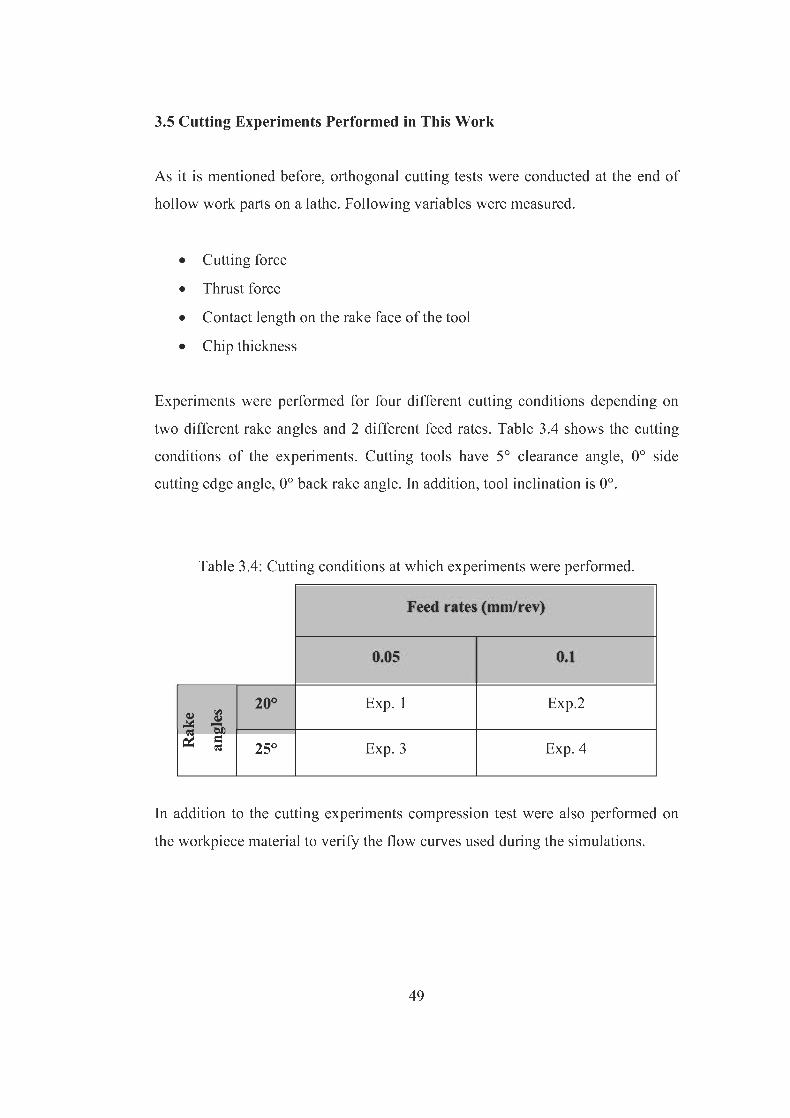
CHAPTER 3

EXPERIMENTAL WORK

3.1 Introduction

The purpose of the experiments performed in this work is to verify the results of

numerical solution obtained by the finite element method. During experiments,

following items were measured:

• Cutting force,

• Thrust force,

• Contact length between the chip and rake face of the tool,

• Chip thickness.

In addition, for every experiment, sample chips were collected and their

thicknesses were measured on a microscope. Therefore, chip thicknesses as well

as the calculated shear angles from the measurements were compared with the

numerical solutions by finite element method.

Simulation results are also compared with experimental results found in

literature, as well as with those obtained in this experimental work.

39

Figure 3.2: Orthogonal turning operation on a lathe.

In this work, the latter one is used. The important thing here is that, wall

thickness, which is depth of cut in this case, must be significantly larger than the

feed rate (undeformed chip thickness when side cutting edge angle is 0°) to

satisfy the plane-strain assumption of finite element model.

3.3 Workpiece Material

Workpiece is a hollow cylinder made of C15 steel. This is a low carbon steel

whose corresponding AISI standard designation is 1015. The outer and inner

diameters of the workpiece are 56 and 53.1 millimeters respectively. Therefore,

the depth of cut is 1.45 millimeters.

Table 3.1 and Table 3.2 show chemical composition and mechanical properties of

the workpiece material.

Table 3.1: Chemical composition of C15 steel in weight percent.

C Si Mn

0.15 0.20 0.45

41

Table 3.2: Mechanical and thermal properties of the workpiece material, C15

steel.

Poisson’s Ratio

Density (g/cm3)

Modulus of

Elasticity (GPa)

Thermal Conductivity

(W/m.K)

Specific Heat

(J/g.K)

Coefficient of Thermal

Expansion (m/m.K)

0.3 7.85 210 58.6 0.46 14.9x10-6

3.4 Test Setup

All cutting experiments were done on a universal lathe (Figure 3.3) with the

cutting speed and feed rate being selected from the available options, which can

be supplied automatically by the machine.

Figure 3.3: Test Setup

Force measurements are taken by means of a dynamometer which can be seen on

Figure 3.4. It is composed of a cutting tool mounted on a horizontal column

whose deflections in both of the horizontal and vertical directions are measured

42

by means of two mercer probes. The dynamometer itself is made of cast iron and

able measure tangential forces up to 2500 N.

Figure 3.4: Lathe tool dynamometer setup.

Mercer probes have a maximum total tip travel of 4.5 mm. Their linearity over

the measuring range is 0.1%. In addition, the repeatability value of these probes is

given as 0.1 µm.

Measured deflections are sent to the analog display, where they can be seen in

micrometers. This display can be scaled to different ranges, making it easier to

read the data. Available ranges are 1500, 500, 150, 50, 15 and 5 µm. The

photograph of the analog display can be seen on Figure 3.5.

43

Figure 3.5: Analog display of the dynamometer.

Since the forces are not measured directly and they are found via the deflection of

the horizontal column, a careful calibration of the dynamometer is needed.

The calibration is done by applying known weights and collecting the measured

deflection data, which can be seen on Figure 3.6. The load was varied from 0 to

135 N and the calibration curves were drawn for both loading and unloading

conditions. Therefore if there is any hysterisis in the measurement, it can be seen.

This procedure is applied for both cutting and thrust force measurements.

44

(a) (b)

Figure 3.6: Calibration of the device. (a) thrust force (b) cutting force

At the end, the gathered calibration curves are as shown on Figure 3.7.

0

20

40

60

80

100

120

140

-5 5 15 25 35Deflection (Micrometer)

Load

(N)

Loading

Unloading

Figure 3.7: Calibration curve for cutting force.

45

0

20

40

60

80

100

120

140

160

0 2 4 6Deflection (micrometers)

Load

(N)

8

Loading

Unloading

Figure 3.8: Calibration curve for thrust force.

It can be seen that, although the thrust force calibration curve is good, there is a

very small hysterisis for the tangential force calibration curve. However,

hysterisis is active, where the cutting forces are quite small. In the experiments,

usually the forces are larger, thus they are not affected from this hysterisis. It is

also important that, the lines are very close to a straight line. Therefore, linear

extrapolation may be used for the loads, which are above the range of calibration

curves.

Contact length and chip thickness measurement were done by means of a Topcon

tool maker’s microscope, which is able measure as small as 1 micron.

Specifications of this device can be found in Table 3.3.

46

Table 3.3: Specifications of the Topcon Universal Measuring Microscope.

Measuring

Ranges

Minimum

Divisions

Overall

Accuracies

Longitudinally 200 mm 0.001 mm (2+0.01 L) µ

Transversely 75 mm 0.001 mm (2+0.01 L) µ

Height 60 mm 0.01 mm 10'

Goniometric

Head 360° 1' 30'

Rotary Table 360° 10'' 15'

Dividing Head 360° 5'

Before cutting experiments, rake face of the tool was painted and after the

experiment completed, length of the erased part was measured by mentioned

microscope. Figure 3.9, Figure 3.10 and Figure 3.11 shows contact length on the

tools rake face, the device and a sample chip thickness.

Figure 3.9: Contact length on the rake face of the tool.

47

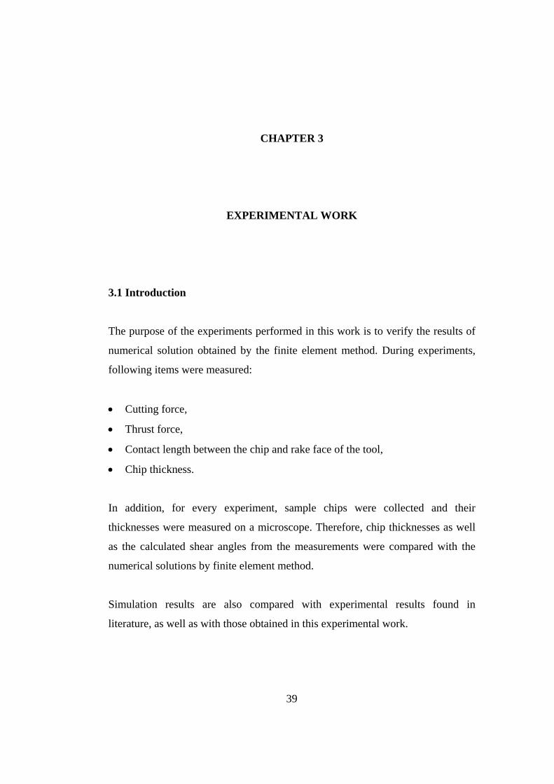
Figure 3.10: Topcon microscope by which the thicknesses of chips were

measured.

Figure 3.11: A sample microscope view while measuring thickness.

48

3.6 Compression Test

As it is mentioned before, cutting experiments were performed with the

workpiece material being C15 (AISI 1015) steel. In the simulations, flow curves

are used from the database of the commercial codes. For the MSC.Marc and

Deform2D they are given in tabular format, whereas Thirdwave AdvantEdge uses

analytical formulation for material flow curve. Therefore, these flow curves need

to be verified for the good representation of material behavior, which is used in

the cutting experiments.

For this purpose, ring compression test were performed on the workpiece

material. The resulted punch displacement – punch force curve were compared

with the simulation of the same process.

At this point it should be noted that, many of the parameters used in analytical

formulation implemented in Thirdwave AdvantEdge are hidden to the user.

Therefore, the comparison of flow curve is not available for Thirdwave

AdvantEdge. Figure-3.12 show the experimentally compressed specimen and the

results of simulations obtained by MSC.Marc and Deform2D.

50

(c)

(b)

(a)

Figu

re 3

.12:

Com

paris

on o

f exp

erim

enta

l and

sim

ulat

ed c

ompr

esse

d sp

ecim

ens.

(a) S

imul

atio

n by

Def

orm

2D (b

) Com

pres

sed

spec

imen

(c) S

imul

atio

n by

MSC

.Mar

c

51

On Figure 3.12, it can be seen that the geometry of the compressed specimen is

estimated very well.

Comparison of punch displacement – punch force diagram can be seen on Figure-

3.13.

0

50000

100000

150000

200000

250000

300000

0.0 1.0 2.0 3.0 4.0 5.0 6.0 7.0 8.0Punch Displacement (mm)

Punc

h Fo

rce

(N)

MSC.Marc

Deform2DExperiment

Figure 3.13: Comparison of punch displacement – punch force diagram.

It is seen that the yield point is estimated very well, although there are small

differences in the plastic region. However this difference might be explained by

the different strain-rates faced during the experiments and available in the flow

curves of commercial codes. Experiments were performed at very small strain-

rates, which are about 4x10-4 s-1. Flow curves, on the other hand does not include

data for such small strain-rates, which leads to about 10 % error in the punch

displacement-punch force curve.

52

CHAPTER 4

NUMERICAL MODEL OF ORTHOGONAL METAL CUTTING

4.1 Introduction

In recent years, finite element method became the main tool for the analysis of

metal cutting. Because it has important advantages, which can be counted as

follows.

• Material properties can be handled as a function of strain, strain-rate, and

temperature

• Nonlinear geometric boundaries, such as free surfaces, can be modeled.

• Other than global variables like cutting force, thrust force; local variables

like strains, strain-rates, stresses, etc. can be obtained

• Interaction of chip and tool can be modeled in different forms.

In this work three different commercial finite element codes were used to model

two dimensional plain-strain orthogonal metal cutting operations. These are

MSC.Marc, Deform2D and Thirdwave AdvantEdge. MSC.Marc and Deform2D

are static implicit codes, whereas Thirdwave AdvantEdge is a dynamic explicit

code.

53

4.2 Finite Element Models

On the following pages, finite element models of all codes will be explained in

different sections. Since three commercial codes have been used, the sections are

as the following:

1. Finite element model of MSC.Marc.

2. Finite element model of Deform2D.

3. Finite element model of Thirdwave AdvantEdge.

At the very end of this chapter, a comparison of all codes will be made in the

sense of finite element formulation, boundary conditions, separation criterion and

etc.

4.2.1 Finite Element Model with MSC.Marc

The model is plane-strain thermo-mechanically coupled and material behavior is

elastic-plastic. The assumption of plane-strain condition is valid if the width of

the cut is significantly larger than the uncut chip thickness. In the model, width of

cut is ten times larger than the uncut chip thickness; therefore the assumption of

plane-strain condition is satisfied.

Figure 4.1: Finite element model of MSC.Marc

54

Figure 4.1 shows the finite element model for MSC.Marc. The workpiece

dimensions are 2 mm in width and 0.5 mm in height. The left and bottom

boundary nodes of the workpiece is restricted so that they can not move in both

of the x and y directions. This is achieved by gluing a stationary rigid curve to

those nodes. This could also be done by defining boundary conditions; however

MSC.Marc can not handle this, when global remeshing is enabled. Hence, rigid

curves have been used to satisfy the necessary boundary conditions. The top and

right boundaries were left as free surfaces.

Figure 4.2: Quadrilateral element

Workpiece was discritized by bilinear quadrilateral elements, which can be seen

on Figure 4.2. Element type is 11, which is written for plane-strain applications,

from MSC.Marc Element Library.

In this work, it is assumed that the tool is not plastifying. Hence it is considered

as rigid and modeled as a curve. Its parameters are rake angle, clearance angle

and cutting edge roundness. Although the rake angle is changing in different

simulations according to the cutting conditions for which it is done, the clearance

angle and nose radius is constant in all of the simulations carried out in this work.

The value of clearance angle is 5° and the value of edge roundness is 0.002 mm.

55

Since this is a thermo-mechanically coupled model, there are also thermal

boundary conditions defined. First of all, the workpiece is loosing heat to the

environment, which is assumed to be at 20 °C, at a rate of 0.4 N/mm.°C.

Workpiece loses heat to the environment due to convection according to the

following formula.

0( )wq h T T= ⋅ − (4.1)

where, h is the convection heat transfer coefficient of the workpiece (0.4

N/(mm.˚C)), Tw is the workpiece surface temperature, and To is the ambient

temperature (20 C˚).

On the other hand, the heat is generated due to two reasons.

• Due to the heavy plastic work done at the shear zone. It is assumed that,

90% of all plastic work is converted into heat.

• Due to friction at the interface of tool and chip.

The half of the generated heat due to friction at the tool chip interface is given to

each of the two contacting bodies, which are chip and tool in this case (Figure

4.3).

56

Figure 4.3: Distribution of generated heat due to friction.

Heat generated due to friction is given by the following formula:

fr rq F v M= ⋅ ⋅ (4.2)

where, Ffr is the friction force, vr is the relative sliding velocity between tool and

chip, and M is the mechanical equivalent of heat (M=1.0).

The rate of specific volumetric flux due to plastic work is given by the following

formula:

pM f WRρ

⋅ ⋅= (4.3)

57

where, Wp is the rate of plastic work, f is the fraction of plastic work converted

into heat which is assumed to be 0.9, M is the mechanical equivalent of heat

(taken as 1.0 by default) and ρ is the density of workpiece material (7.85 g/cm3).

The workpiece material used for this plane-strain orthogonal metal cutting

simulation is C15 steel. Its flow curve is represented by several tabulated data

(MSC.Marc database) which depends on strain, strain-rate and temperature.

The material data is represented by several flow curves at 3 different strain-rates

(1.6, 8 and 40 s-1) and at 13 different temperatures (20, 100, 200, 300, 400, 500,

600, 700, 800, 900, 1000, 1100, 1200 ˚C), while strain is changing between 0 and

1. Figure 4.4, 4.5 and 4.6 shows the flow curves of the material for different

strain rates.

0

100

200

300

400

500

600

700

800

900

1000

0 0.1 0.2 0.3 0.4 0.5 0.6 0.7 0.8 0.9 1

Equivalent Plastic Strain

Flow

Str

ess

(MPa

)

T=20 °C T=200 °CT=400 °C

T=500 °C

T=300 °C

T=100 °C

T=600 °C

T=700 °C

T=800 °C

T=900 °C T=1000 °CT=1100 °C T=1200 °C

Figure 4.4: Workpiece flow curve for strain-rate of 40 (s-1).

58

59

0

100

200

300

400

500

600

700

800

900

1000

0 0.1 0.2 0.3 0.4 0.5 0.6 0.7 0.8 0.9 1Equivalent Plastic Strain

Flow

Str

ess

(MPa

)

T=20 °C

T=300 T=200 °CT=100 °CT=400 °C

T=500 °C

T=600 °CT=700 °CT=800 °C

T=1000 °CT=1100

T=1200 °C

T=900 °C

Figure 4.5: Workpiece flow curve for strain-rate of 8 (s-1).

0

100

200

300

400

500

600

700

800

900

1000

0 0.1 0.2 0.3 0.4 0.5 0.6 0.7 0.8 0.9 1

Equivalent Plastic Strain

Flow

Str

ess

(MPa

)

T=200 °CT=300 °C

T=20 °CT=100 °C

T=400 °C

T=500 °CT=600 °C

T=700 °CT=800 °CT=900 °C

T=1000 °CT=1100 °CT=1200 °C

Figure 4.6: Workpiece flow curve for strain-rate of 1.6 (s-1).

In the cutting process, the deformation of material at the cutting zone takes place

at elevated temperatures and strain rates. However, if the given flow curves are

exceeded, then required data is calculated at the border. Therefore, after

exceeding the highest value of strain-rate available, calculations are always done

using the same flow curve set, which, in this case, the one available for 40 s-1.

This is the weakest point of this finite element model. Although the strain-rates at

the shear zone can be extremely high, the flow stress of the material can only be

calculated at a maximum strain-rate of 40 s-1.

0

100

200

300

400

500

600

700

0 0.1 0.2 0.3 0.4 0.5 0.6 0.7 0.8 0.9 1

Equivalent Plastic Strain

Flow

Str

ess (

MPa

)

Figure 4.7: Effect of strain-rate on the flow curves.

Figure-4.7 is flow curves of the workpiece material at 500 °C and at different

strain-rates. This figure can give an idea of error introduced by improper flow

stress evaluation at elevated strain-rates.

In the simulations, the tool is pushed to penetrate through the workpiece at the

cutting speed. The friction between the tool and the chip is modeled as constant

60

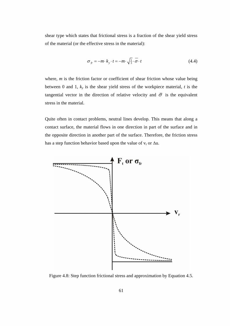
shear type which states that frictional stress is a fraction of the shear yield stress

of the material (or the effective stress in the material):

13fr ym k t m tσ σ= − ⋅ ⋅ = − ⋅ ⋅ ⋅ (4.4)

where, m is the friction factor or coefficient of shear friction whose value being

between 0 and 1, ky is the shear yield stress of the workpiece material, t is the

tangential vector in the direction of relative velocity and σ is the equivalent

stress in the material.

Quite often in contact problems, neutral lines develop. This means that along a

contact surface, the material flows in one direction in part of the surface and in

the opposite direction in another part of the surface. Therefore, the friction stress

has a step function behavior based upon the value of vr or ∆u.

Figure 4.8: Step function frictional stress and approximation by Equation 4.5.

61

This discontinuity in the value of σfr can result in numerical difficulties, so a

modified Constant Shear friction model is implemented in MSC.Marc whose

formula is given as:

12 tan3

rfr

vm tC

σσπ

− ⎛ ⎞= − ⋅ ⋅ ⋅ ⋅⎜ ⎟⎝ ⎠

(4.5)

where, vr is the magnitude of relative velocity between the die and the workpiece

and C is a constant, named relative sliding velocity.

Figure 4.8 show the step function behavior of friction (solid line) and its

approximation by Equation 4.5 (dash lines). Depending on the value of C, degree

of approximation can be changed.

Physically, C has the value of the relative velocity when sliding occurs. The value

of C is important in determining how closely the mathematical model represents

the step function. A very large value of C results in a reduced value of the

effective friction. On the other hand, a very small value results in poor

convergence. It is recommended that the value of C be 1% or 10% of a typical

relative sliding velocity, vr. Because of this smoothing procedure, a node in

contact always has some slipping.

In this work, the value of the coefficient of shear friction has been changed in the

range of 0.2 to 0.7 to see the effects on the process results like shear angle,

cutting force, thrust force, and etc. The value of C was taken as 1 % of the

magnitude of the relative sliding velocity between the chip and tool.

As already discussed in the Chapter 2, (Literature survey), there are a number of

methods to separate material from the workpiece to form the chip while the tool

penetrates into it. In this model, the method of remeshing was applied. Therefore,

the workpiece is remeshed whenever the tool penetrates into the workpiece by a

62

predefined threshold value. Figure 4.9 shows how a new surface is generated on

the workpiece by remeshing when a penetration occurs.

Figure 4.9: Separation of chip from the workpiece by continuous remeshing.

By default MSC.Marc takes penetration value as 0.05 of the minimum element

edge length, however it is possible to change it. In addition, the time of

penetration check can also be altered, being either at the end of increments, or at

every iteration. Although the penetration value does not introduce a significant

difference, the type penetration check leads to major changes in the results. The

effects of these two variables can be seen in Chapter 5 (Results and Comparison).

4.2.2 Finite Element Model with Deform2D

The model of Deform2D is not so different than the model of MSC.Marc. This is

again a thermo-mechanically coupled simulation with elastic-plastic material

modeling. There are two differences between the models of MSC.Marc and

Deform2D:

63

1. The method used to satisfy the necessary boundary conditions on the bottom

and left boundary nodes of the workpiece.

2. The method used to separate the chip from the workpiece.

Figure 4.10 shows the finite element model of orthogonal cutting, which is used

with Deform2D.

Figure 4.10: Finite element model of Deform2D.

Deform2D is able to handle global remeshing when there is displacement

boundary conditions defined for the workpiece. Therefore, in the model with

Deform2D, the left boundary nodes are fixed in x-direction, and the bottom

boundary nodes are fixed in y-direction.

As it is the case with MSC.Marc, in the simulation with Deform2D, the tool was

pushed to penetrate through the workpiece to form the chip. However, the

formation of chip is different for Deform2D. The idea is that, while the tool

penetrates, the elements at the tip of the tool are erased via remeshing whenever

they reach a critical damage value. Figure 4.11 shows an element erase stage

during the two consequent increments of simulation. It can be seen that, element

is erased and the workpiece is remeshed.

64

Figure 4.11: Element erase due to damage via remeshing in Deform2D

In Deform2D, different damage models can be defined and among those

Normalized Cockroft-Latham damage criterion was used to initiate deletion of

elements for separating the chip from the workpiece. Critical damage value, C, is

used as 0.2, which is found from literature.

Workpiece dimensions are again 2 mm in width and 0.5 mm in height. It was

discritized by bilinear quadrilateral elements (Figure 4.2).

65

Thermal boundary conditions were defined to enable the coupling of thermal and

mechanical solutions:

1. Heat is generated due to plastic work done on the workpiece while the tool

penetrates through the material (Equation 4.3). It is assumed that 90% of all

plastic work is converted into heat.

2. Heat is generated due to friction between the tool and the chip (Equation 4.2).

3. The workpiece is loosing heat to the environment (Equation 4.1). The value

of convection coefficient, h, is taken as 0.4 (N.mm/°C) and the ambient

temperature is assumed to be at 20 °C.

Workpiece material was chosen as 0.15 % Carbon steel from the database of

Deform2D. This database includes only the flow stress of the chosen material.

Therefore, the other input data should be entered separately, such as elastic

modulus, poison’s ratio, thermal expansion coefficient, thermal conduction

coefficient and heat capacity of the material. If the simulation conditions of the

material exceed the bounds of the strain, strain rate or temperature defined in the

tabular data, Deform2D extrapolates the tabulated data based on the last two data

points to find the desired flow stress.

Friction between the tool’s rake face and chip is modeled by the constant shear

law, which is the same as the model of MSC.Marc. The friction factor has been

changed between 0.2 and 0.7 to see the effects of friction on the process

variables.

4.2.3 Finite Element Model with Thirdwave Systems Advantedge

Thirdwave Systems Advantedge is a special program written only for machining

simulations. It is a dynamic explicit Lagrangian formulation. The model is built

66

by selecting the type of machining operation (e.g. turning, broaching, sawing or

milling) and defining the necessary process parameters. Since the main subject of

this work is turning operations, the process parameters that should be inputted to

Advantedge are feed rate, depth of cut, length of cut, cutting speed and initial

temperature of the workpiece. Other parameters are fixed automatically by the

code and hidden to the user..

Figure 4.12: Finite element model of Third Wave Systems AdvantEdge.

Figure 4.12 shows both the turning operation itself and the two dimensional

modeling in Thirdwave AdvantEdge. On this figure, lc is the length of cut, f is the

feed rate and V is the cutting speed. Depth of cut is defined as the dimension to

the inside of the paper.

67

This model is also thermo-mechanically coupled. In Advantedge a staggered

procedure is adopted for the purpose of coupling the thermal and mechanical

equations. Geometrically identical meshes for the thermal and mechanical models

are used. Mechanical and thermal computations are staggered assuming constant

temperature during the mechanical step and constant heat generation during the

thermal step. A mechanical step is taken first based on the current distribution of

temperatures, and the heat generated is computed from plastic working and

frictional heat generation. The heat thus computed is transferred to the thermal

mesh and the temperatures are recomputed by recourse to the forward-Euler

algorithm. The resulting temperatures are transferred to the mechanical mesh and

are incorporated into the thermal-softening model, which completes one time-

stepping cycle.

Thermal boundary conditions for Thirdwave AdvantEdge are given as:

1. The heat is generated due to heavy plastic work done on the workpiece,

whose formula is given in Equation 4.3.

2. The heat is generated due to friction between the chip and the rake face of the

tool according to Equation 4.2.

3. The generated frictional heat is distributed to chip and tool according to the

Equation 4.6, where Qchip is the heat given to the chip, Qtool is the heat given

to the tool, Qfriction is the total heat generated due to friction, k is the

conductivity, ρ is the density and c is the heat capacity.

chip chip chipchip

tool tool tool tool

chip tool friction

k cQQ k c

and

Q Q Q

ρ

ρ

⋅ ⋅=

⋅ ⋅

+ =

(4.6)

68

The finite deformation formulation in Third Wave AdvantEdge incorporates six-

noded quadratic triangular elements for the spatial discretization. The element has

three corner and three mid-side nodes providing quadratic interpolation of the

displacements within the element.

Figure 4.13: Six-noded triangular element.

The separation of nodes, thus forming the chip from the workpiece during a

cutting simulation is achieved by continuous remeshing, which is also applied for

the simulations with MSC.Marc. Therefore, during metal cutting the workpiece

material is allowed to flow around the cutting tool edge and when the elements in

this vicinity become distorted and lose accuracy, Thirdwave AdvantEdge

alleviates element distortion by updating the finite element mesh periodically by

refining large elements, remeshing distorted elements, and coarsening small

elements.

As it is mentioned before, in a typical machining event, very high strain rates, in

excess of 104 s-1 may be attained within the primary and secondary shear zones,

while the remainder of the workpiece deforms at moderate or low strain rates. In

order to account for a variation in the strain rate sensitivity at low and high strain

rates, AdvantEdge incorporates a stepwise variation of the rate sensitivity

69

exponent m while maintaining continuity of stress. This leads to the following

relations for low and high strain-rates.

( )1

1

p

0

1 , mp

p pf tp ifεσ σ ε ε ε

ε⎛ ⎞

= ⋅ + ≤⎜ ⎟⎝ ⎠

(4.7)

( )2 1

1 1

0 0

1 1 , m mp

p pt pf tp p ifεεσ σ ε ε ε

ε ε⎛ ⎞ ⎛ ⎞

= ⋅ + ⋅ + >⎜ ⎟ ⎜ ⎟⎝ ⎠ ⎝ ⎠

(4.8)

where, σ is the effective Von-Mises stress, fσ is the flow stress, pε is the

accumulated plastic strain, 0pε is a reference plastic strain rate, m1 and m2 are low

and high strain-rate sensitivity exponents respectively and tε is the threshold

strain-rate which separates the two regimes. In calculations, a local Newton-

Raphson iteration is used to compute 0pε according to the low-rate equation, and

switches to the high rate equation if the result lies above tε .

AdvantEdge uses an adopted power hardening law with thermal softening with

the governing equation being as the following.

( )1

00

1np

f pT T εσ σε

⎛ ⎞= ⋅ ⋅ +⎜ ⎟

⎝ ⎠ (4.9)

where, n is the hardening exponent, T is the current temperature, 0σ is the initial

yield stress at the reference temperature T0, 0pε is the reference plastic strain, T(T)

is a thermal softening factor ranging from 0 to 1 and has a general representation

depending on the workpiece material of interest.

70

CHAPTER 5

RESULTS AND COMPARISON

5.1 Introduction

Finite element simulations were carried out for 4 cases of experiments composing

of 2 different rake angles and 2 different feed rates with MSC.Marc,

DEFORM2D and Thirdwave AdvantEdge separately. Table 5.1 shows the

different cutting conditions under which simulations were carried out. It should

be noted that, due to a repeated software crash, simulation 3 of Deform2D could

not be completed. Hence, the results of this simulation will not be available on

the charts related with Deform2D.

Table 5.1: Simulations were done under four different cutting conditions.

Feed Rates (rev/min) 0.05 0.1

20° Sim-1 Sim-2

Rak

e A

ngle

s

25° Sim-3 Sim-4

In all simulations, it is made sure that steady state has reached and some more

data is collected after that time. Figure 5.1 shows a typical cutting force versus

increment number graph, where it can be seen that after some point steady-state is

72

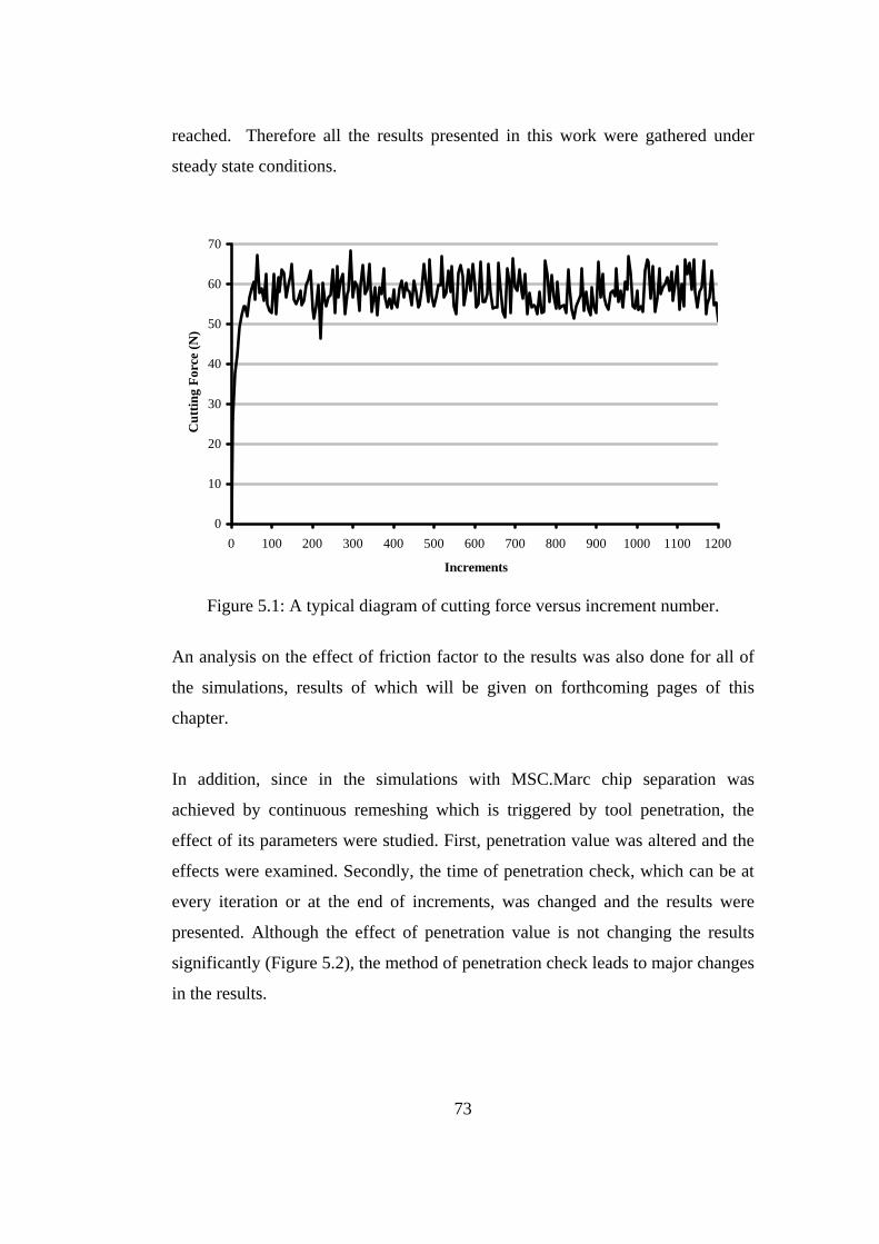
reached. Therefore all the results presented in this work were gathered under

steady state conditions.

0

10

20

30

40

50

60

70

0 100 200 300 400 500 600 700 800 900 1000 1100 1200

Increments

Cut

ting

Forc

e (N

)

Figure 5.1: A typical diagram of cutting force versus increment number.

An analysis on the effect of friction factor to the results was also done for all of

the simulations, results of which will be given on forthcoming pages of this

chapter.

In addition, since in the simulations with MSC.Marc chip separation was

achieved by continuous remeshing which is triggered by tool penetration, the

effect of its parameters were studied. First, penetration value was altered and the

effects were examined. Secondly, the time of penetration check, which can be at

every iteration or at the end of increments, was changed and the results were

presented. Although the effect of penetration value is not changing the results

significantly (Figure 5.2), the method of penetration check leads to major changes

in the results.

73

0

10

20

30

40

50

60

70

80

0 25 50 75 100 125 150 175 200 225 250 275 300Increments

Cut

ting

Forc

e (N

)

Default Penetration ValuePenetration Value=0.001

Figure 5.2: Effect of contact penetration value.

0

10

20

30

40

50

60

70

80

0 25 50 75 100 125 150 175 200 225 250 275 300

Increments

Cut

ting

Forc

e (N

)

Default Penetration Value, End of Increment CheckDefault Penetration Value, Per Iteration Check

True Value

Figure 5.3: Effect of penetration check method on the results.

74

Figure 5.3 shows the cutting force results with two different penetration check

methods for the same simulation. The simulation, in which the penetration is

checked at every iteration gives results, which are almost half of the results

obtained by the other method..

From the simulations, variables like stresses, strains, strain rates and temperature

distribution can be obtained. However, these are all very difficult to measure

experimentally. On the other hand, cutting force and thrust force can be measured

relatively easily. In addition to this, contact length of chip on the rake face and

the thickness of the chips, from which the shear angle can be found, can be

measured.

Therefore, in this chapter, cutting force, thrust force, chip thickness, contact

length and shear angle found from own experiments are compared with the

simulations of three commercial codes. Also experimental results from literature

are compared with the simulations. In addition, the results of simulations are

verified with analytical solutions available.

5.2 Comparison with Analytical Solutions

Slip-line models by Lee & Shaffer [13], Kudo [18] and Dewhurst [19] gives an

allowable range for the possible solutions of the relation between φ, γ, β. where φ,

γ, β denotes shear plane angle, rake angle of the tool and chip-tool friction angle

respectively. The diagrammatic view of these angles can be seen on Figure 5.4. In

this study, diagrams have been drawn (φ – γ) against β according to Hill’s [17]

overstressing criterion as suggested by Childs [63]. Figure 5.5 and Figure 5.6

show allowable ranges for the rake angles of 20° and 25° respectively.

75

0

10

20

30

40

50

0 10 20 30 40 50Friction Angle

Shea

r A

ngle

- R

ake

Ang

leKudo

Dewhurst

Lee & Shaffer

Simulation Results

Figure 5.6: Allowable slip-line model solutions for rake angle of 25°.

The graphs also contain the simulation results of MSC.Marc. All the results are

between the upper and lower bounds suggested by Kudo and Dewhurst

respectively. The graph also shows that, Lee and Shaffer model, which is

relatively simple than the others, gives good predictions. Especially for the rake

angle of 20°, simulated results are almost coincident with the suggested solution

of Lee and Shaffer.

5.3 Comparison of Chip Geometry

As it is mentioned before, thickness of the cut chips and contact lengths between

the chip and rake face of the tool were measured by means of a microscope.

Table 5.2 shows the experimental results, where γ is the rake angle, f is the feed

rate (uncut chip thickness for 0° side cutting edge angle), a0 is the chip thickness,

φ is the shear angle and lc is the contact length between the chip and the rake face

of the tool.

77

Figure 5.7: Shear angle can be found from strain-rate distribution.

Second method is that, it can be calculated from the computed chip thicknesses.

Equation 1 gives shear angle as depended on rake angle and chip thickness ratio.

( ) ( )( )

costan

1 sinc

c

rr

γϕ

γ⋅

=− ⋅

(1)

where, φ is the shear angle, γ is the rake angle, and rc is the chip thickness ratio,

which is defined as the ratio of uncut chip thickness to cut chip thickness.

Results show that, although both are in good agreement, strain-rate distribution

gives a better estimation of the shear angle. Contact lengths, on the other hand,

are very poorly estimated.

Figure 5.8, Figure 5.9 and Figure 5.10 show the chip thickness, shear angle

calculated from chip thickness results and contact length estimations of

MSC.Marc in comparison with experiments, respectively. It can be seen that

79

there is a gradual convergence to the experimental results with increasing friction

factor.

Exp

erim

ent

Exp

erim

ent

Exp

erim

ent

m=0

.2

m=0

.2

m=0

.2

m=0

.2

m=0

.4

m=0

.4

m=0

.4

m=0

.4

m=0

.7

m=0

.7

m=0

.7

m=0

.7

Exp

erim

ent

0.00

0.05

0.10

0.15

0.20

0.25

0.30

Chi

p T

hick

ness

(mm

)

γ=20°f=0.05 mm/rev

γ=20°f=0.1 mm/rev

γ=25°f=0.05 mm/rev

γ=25°f=0.1 mm/rev

Figure 5.8: Effect of friction factor on the chip thickness results obtained by

MSC.Marc.

Exp

erim

ent

Exp

erim

ent

Exp

erim

ent

m=0

.2

m=0

.2

m=0

.2

m=0

.2

m=0

.4

m=0

.4

m=0

.4

m=0

.4

m=0

.7

m=0

.7

m=0

.7

m=0

.7

Exp

erim

ent

0

5

10

15

20

25

30

35

40

45

Shea

r A

ngle

(deg

rees

)

γ=20°f=0.05 mm/rev

γ=20°f=0.1 mm/rev

γ=25°f=0.05 mm/rev

γ=25°f=0.1 mm/rev

Figure 5.9: Effect of friction factor on the shear angles obtained by MSC.Marc

calculated from chip thickness results.

80

them, are not also in agreement with the experiments. On the other hand, strain-

rate distribution gives better results. Contact lengths are again very poorly

estimated.

Figure 5.11, Figure 5.12 and Figure 5.13 show the chip thickness, shear angle

calculated from chip thickness estimation and contact length computations in

comparison with experimental results, respectively.

Exp

erim

ent

Exp

erim

ent

Exp

erim

ent

m=0

.2 m=0

.2

m=0

.2

m=0

.4 m=0

.4

m=0

.4 m=0

.4

m=0

.7 m=0

.7

m=0

.7 m=0

.7

Exp

erim

ent

0.00

0.05

0.10

0.15

0.20

0.25

0.30

Chi

p T

hick

ness

(mm

)

γ=20°f=0.05 mm/rev

γ=20°f=0.1 mm/rev

γ=25°f=0.05 mm/rev

γ=25°f=0.1 mm/rev

Figure 5.11: Effect of friction factor on the chip thickness results with Deform2D.

82

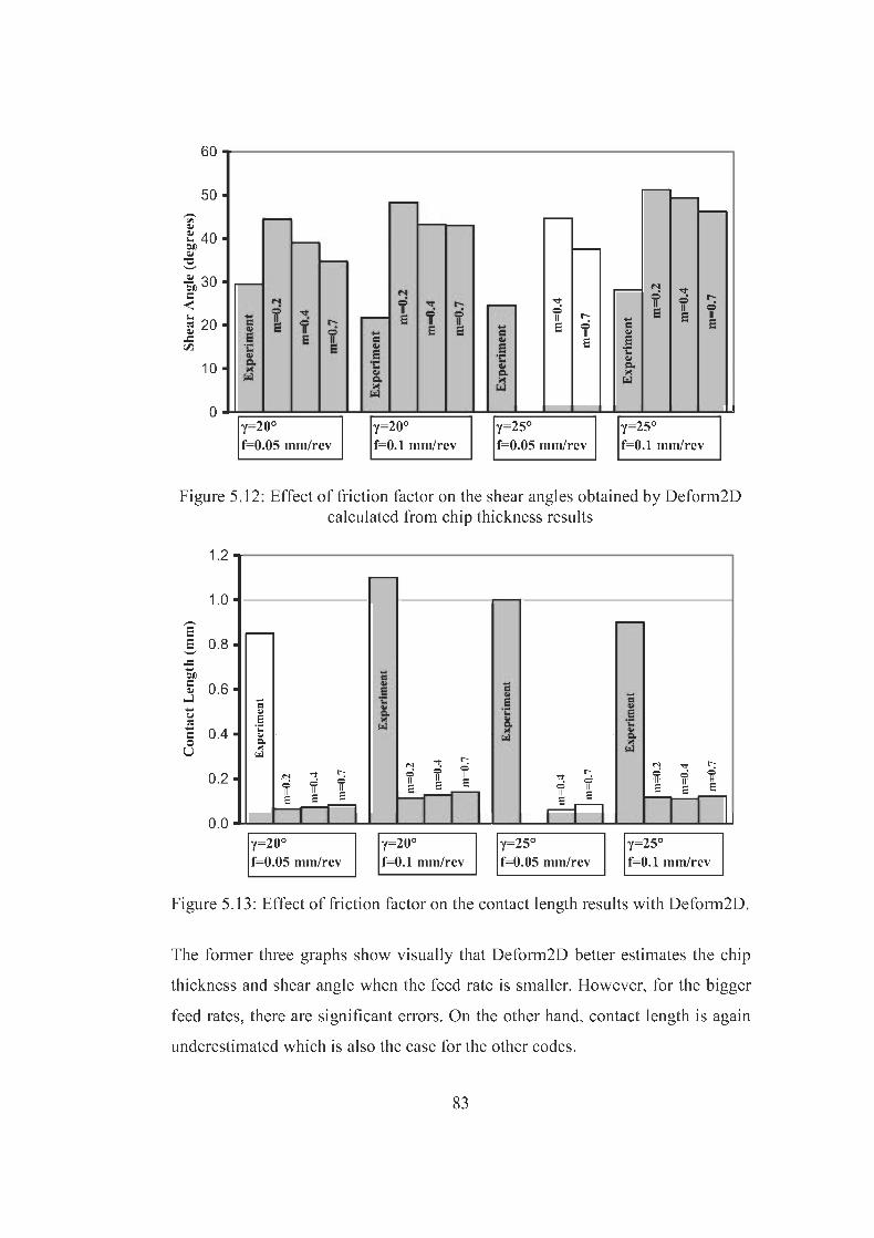
Exp

erim

ent

Exp

erim

ent

Exp

erim

ent

Exp

erim

ent µ=0

.2

µ=0

.2

µ=0

.2

µ=0

.2

µ=0

.4

µ=0

.4

µ=0

.4

µ=0

.4

µ=0

.5

µ=0

.5

µ=0

.5

µ=0

.5

0.00

0.05

0.10

0.15

0.20

0.25

0.30

Chi

p T

hick

ness

(mm

)

γ=20°f=0.05 mm/rev

γ=20°f=0.1 mm/rev

γ=25°f=0.05 mm/rev

γ=25°f=0.1 mm/rev

Figure 5.14: Effect of friction factor on the chip thickness results with

Thirdwave AdvantEdge.

Exp

erim

ent

Exp

erim

ent

Exp

erim

ent

Exp

erim

ent

µ=0

.2

µ=0

.2

µ=0

.2

µ=0

.2

µ=0

.4

µ=0

.4

µ=0

.4

µ=0

.4

µ=0

.5

µ=0

.5

µ=0

.5

µ=0

.5

0

5

10

15

20

25

30

35

40

Shea

r A

ngle

(deg

rees

)

γ=20°f=0.05 mm/rev

γ=20°f=0.1 mm/rev

γ=25°f=0.05 mm/rev

γ=25°f=0.1 mm/rev

Figure 5.15: Effect of friction factor on the shear angles obtained by Thirdwave AdvantEdge calculated from chip thickness results

85

Exp

erim

ent

Exp

erim

ent

Exp

erim

ent

Exp

erim

ent

µ=0

.2

µ=0

.2µ=0

.2

µ=0

.2 µ=0

.4

µ=0

.4µ=0

.4

µ=0

.4 µ=0

.5

µ=0

.5µ=0

.5

µ=0

.5

0.0

0.2

0.4

0.6

0.8

1.0

1.2

Con

tact

Len

gth

(mm

)

γ=20°f=0.05 mm/rev

γ=20°f=0.1 mm/rev

γ=25°f=0.05 mm/rev

γ=25°f=0.1 mm/rev

Figure 5.16: Effect of friction factor on the contact length by Thirdwave

AdvantEdge

The results of both chip thickness and shear angle are in very good agreement

with the experiments. As it is mentioned before, this program uses Coulomb

friction model and the chip geometry results are best estimated when the friction

coefficient is taken as 0.5. On the other hand, contact lengths are significantly

different from the results of experiments, which was also the case with

MSC.Marc and Deform2D. In addition, some inconsistencies also exist in the

results of Thirdwave AdvantEdge. For example, although the chip thickness is

generally underestimated by the code, for the cutting condition, where rake angle

is 20° and feed rate is 0.05 mm/rev, it is overestimated after a friction coefficient

of 0.4.

Figure 5.17, Figure 5.18 and Figure 5.19 show the results of chip thickness, shear

angle calculated from chip thickness estimation and contact length respectively

from all of the three codes with their best estimations in comparison with

experimental results.

86

Exp

erim

ent

Exp

erim

ent

Exp

erim

ent

MSC

.Mar

c MSC

.Mar

c

MSC

.Mar

c MSC

.Mar

c

Def

orm

2D

Def

orm

2D

Def

orm

2D

Def

orm

2D

Adv

antE

dge Adv

antE

dge

Adv

antE

dge

Adv

antE

dge

Exp

erim

ent

0.00

0.05

0.10

0.15

0.20

0.25

0.30

Chi

p T

hick

ness

(mm

)

γ=20°f=0.05 mm/rev

γ=20°f=0.1 mm/rev

γ=25°f=0.05 mm/rev

γ=25°f=0.1 mm/rev

Figure 5.17: Comparison of chip thickness results from three codes with experiments. m=0.7 for MSC.Marc and Deform2D and µ=0.5 Thirdwave

AdvantEdge

Exp

erim

ent

Exp

erim

ent

Exp

erim

ent

MSC

.Mar

c

MSC

.Mar

c

MSC

.Mar

c

MSC

.Mar

c

Def

orm

2D

Def

orm

2D

Def

orm

2D

Def

orm

2D

Adv

antE

dge

Adv

antE

dge

Adv

antE

dge

Adv

antE

dge

Exp

erim

ent

0

5

10

15

20

25

30

35

40

45

50

Shea

r A

ngle

(deg

rees

)

γ=20°f=0.05 mm/rev

γ=20°f=0.1 mm/rev

γ=25°f=0.05 mm/rev

γ=25°f=0.1 mm/rev

Figure 5.18: Shear angles obtained by three codes by calculating from chip

thickness estimation. m=0.7 for MSC.Marc and Deform2D and µ=0.5 Thirdwave AdvantEdge

87

Exp

erim

ent

Exp

erim

ent

Exp

erim

ent

MSC

.Mar

c

MSC

.Mar

c

MSC

.Mar

c

MSC

.Mar

c

Def

orm

2D

Def

orm

2D

Def

orm

2D

Def

orm

2D

Adv

antE

dge

Adv

antE

dge

Adv

antE

dge

Adv

antE

dge

Exp

erim

ent

0.0

0.2

0.4

0.6

0.8

1.0

1.2

Con

tact

Len

gth

(mm

)

γ=20°f=0.05 mm/rev

γ=20°f=0.1 mm/rev

γ=25°f=0.05 mm/rev

γ=25°f=0.1 mm/rev

Figure 5.19: Comparison of contact length results of codes with experiments.

m=0.7 for MSC.Marc and Deform2D and µ=0.5 Thirdwave AdvantEdge

In the view of above results, it can be concluded that, the three commercial codes

estimate the chip thickness, and shear angle quite well. However, the estimation

of contact length between the chip and rake face of the tool is not in agreement

with the experiments for all of the codes.

In addition, although the results of MSC.Marc and Thirdwave AdvantEdge are

similar to each other, Deform2D generally predicts different values than the other

two commercial codes. The reason behind this fact might be the use of a different

chip separation criterion. Because, as it is already explained in Numerical

Modeling of Orthogonal Metal Cutting Chapter, MSC.Marc and Thirdwave

AdvantEdge separates the chip from the workpiece by continuous remeshing,

whereas, Deform2D uses Cockroft-Latham damage criterion to erase the

elements at the tool tip which exceed a predefined damage value.

88

Table 5.6: Cutting conditions for the chip geometry verification.

γ° α°

f

(mm/rev)

dc

(mm)

Vc

(rev/min) m µ

1 20°

2 25° 5° 0.1 1.45 125 0.7 0.5

Figure 5.20 (a), (b) and (c) show simulated chip geometries as computed by

MSC.Marc (m=0.7), Deform2D (m=0.7) and Thirdwave AdvantEdge

(µ=0.5)respectively. All the pictures were drawn for the same tool stroke, so that,

they are comparable with each other. Cutting conditions are as given in the first

row of Table 5.6, where γ is the rake angle, β is the clearance angle, f is the feed

rate, dc is the depth of cut and Vc is the cutting speed. Figure 5.21, on the other

hand, shows simulated chip geometries from three codes when the rake angle has

been changed to 25°, while the other cutting conditions were kept constant.

89

(a)

(b)

(c)

Figure 5.20: Simulated chip geometries from three commercial codes at 20° rake angle.

(a) MSC.Marc (m=0.7), (b) Deform2D (m=0.7), (c) Thirdwave AdvantEdge

(µ=0.5).

90

(a)

(b)

(c)

Figure 5.21: Simulated chip geometries with three commercial codes at 25° rake angle

(a) MSC.Marc (m=0.7), (b) Deform2D (m=0.7), (c) Thirdwave AdvantEdge

(µ=0.5).

91

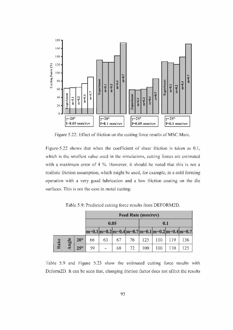
Exp

erim

ent

Exp

erim

ent

Exp

erim

ent

Exp

erim

ent

µ=0.

2

µ=0.

2

µ=0.

2

µ=0.

2

µ=0.

4

µ=0.

4

µ=0.

4

µ=0.

4

µ=0.

5

µ=0.

5

µ=0.

5

µ=0.

5

0

50

100

150

200C

uttin

g Fo

rce

(N)

γ=20°f=0.05 mm/rev

γ=20°f=0.1 mm/rev

γ=25°f=0.05

/

γ=25°f=0.1 mm/rev

Figure 5.24: Effect of friction on the cutting force results of Thirdwave

AdvantEdge. Figure 5.25 shows the comparison of best cutting force estimations obtained by

all of the three commercial codes. Therefore, m=0.7 for MSC.Marc and

Deform2D and µ=0.5 for Thirdwave AdvantEdge.

Exp

erim

ent

Exp

erim

ent

Exp

erim

ent

Exp

erim

ent

MSC

.Mar

c MSC

.Mar

c

MSC

.Mar

c MSC

.Mar

c

Def

orm

2D Def

orm

2D

Def

orm

2D

Def

orm

2D

Adv

antE

dge

Adv

antE

dge Adv

antE

dge

Adv

antE

dge

0

25

50

75

100

125

150

175

200

225

Cut

ting

Forc

e (N

)

γ=20°f=0.05 mm/rev

γ=20°f=0.1 mm/rev

γ=25°f=0.05 mm/rev

γ=25°f=0.1 mm/rev

Figure 5.25: Comparison of cutting forces estimated by three codes and

experiments m=0.7 for MSC.Marc and Deform2D and µ=0.5 for Thirdwave AdvantEdge

95

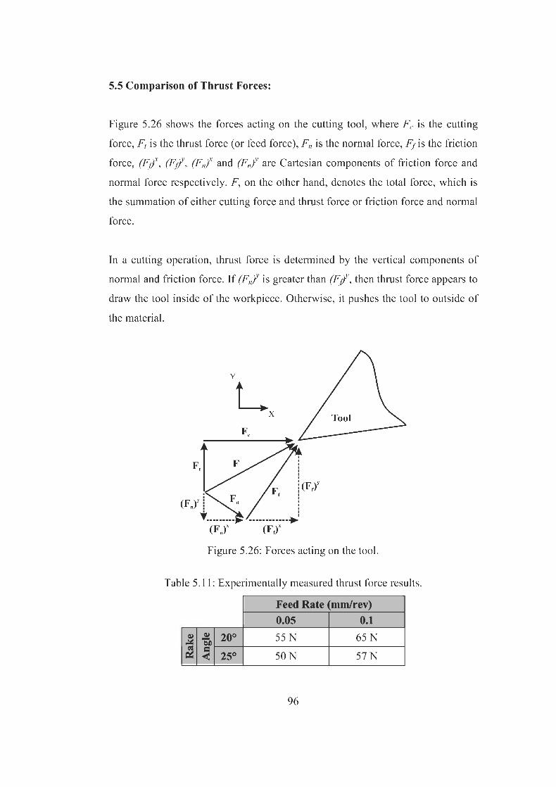
Exp

erim

ent

Exp

erim

ent

Exp

erim

ent

Exp

erim

ent

MSC

.Mar

c

MSC

.Mar

c

MSC

.Mar

c

MSC

.Mar

c

Deform2DDeform2D Deform2D

Deform2D

Adv

antE

dge

Adv

antE

dge

Adv

antE

dge

Adv

antE

dge

-25

0

25

50

75

Cut

ting

Forc

e (N

)

γ=20°f=0.05 mm/rev

γ=20°f=0.1 mm/rev

γ=25°f=0.05 mm/rev

γ=25°f=0.1 mm/rev

Figure 5.30: Comparison of thrust forces estimated by three codes and experiments

m=0.7 for MSC.Marc and Deform2D and µ=0.5 for Thirdwave AdvantEdge

5.6 Comparison of Simulation with the Experimental Results from

Literature

Cutting and thrust forces, shear angle, contact length and temperature distribution

obtained by the model of MSC.Marc in this work are compared with the results

found from literature.

Movahhedy and Altintas [20] did some orthogonal metal cutting experiments

with low carbon steel for the verification of their finite element model in which

they have measured cutting force, thrust force, shear plane angle, contact length

and maximum temperature reached.

Cutting conditions and experimental results as well as the simulation results of

Movahhedy and Altintas can be found in Table 5.15.

100

Table 5.15: Experimental and Simulation results of Movahhedy and Altintas.

γ° Vc(m/min)

f (mm/rev)

dc (mm)

Fc(N)

Ft(N) φ° lc

(mm) Tmax (°C)

Experiment 0° 150 0.1 1 174 83 18.8° 0.6 590 Simulation 0° 150 0.1 1 207 96 22° 0.55 571

Table 5.16 shows the results of this work predicted by MSC.Marc, where friction

factor was taken as 0.1. It can be seen that the predicted thrust force, the shear

angle and the contact length is not in agreement with the experiments. However

cutting force is predicted well. Temperature prediction has an error about 9

percent which can be treated as a good estimation.

Table 5.16: Comparison with literature (m=0.1).

γ° Vc(m/min)

f (mm/rev)

dc (mm)

Fc(N)

Ft(N) φ° lc

(mm) Tmax (°C)

Experiment 0° 150 0.1 1 174 83 18.8° 0.6 590 Simulation 0° 150 0.1 1 174 20 22.1° 0.168 535

Table 5.17, on the other hand, shows the results predicted by MSC.Marc with a

friction factor of 0.7, which is proved to supply better results according to the

comparisons with experiments performed in this work. With this simulation

thrust force prediction becomes quite precise while the cutting force is

overestimated. Shear angle was simulated with an error of about 5 percent.

Temperature prediction becomes even better due to higher heat generation at the

chip tool interface because of higher friction factor. The error is about 7 percent.

Table 5.17: Comparison with literature (m=0.7).

α° Vc(m/min)

f (mm/rev)

dc (mm)

Fc(N)

Ft(N) φ° lc

(mm) Tmax (°C)

Experiment 0° 150 0.1 1 174 83 18.8° 0.6 590 Simulation 0° 150 0.1 1 225 85 17.7° 0.45 547

101

Exp

erim

ent

Exp

erim

ent

m=0.1 m=0.7 m=0.7m=0.10

25

50

75

100

125

150

175

200

225

Forc

e (N

)

Cutting Thrust Forces

Figure 5.31: Comparison of cutting and thrust forces obtained by MSC.Marc with

experiment from literature

Experiment

m=0.1

m=0.7

0

5

10

15

20

25

Shea

r A

ngle

Figure 5.32: Comparison of shear angle obtained by MSC.Marc with experiment

from literature

102

Experiment

m=0.1 m=0.7

0

100

200

300

400

500

600

Max

imum

Tem

pera

ture

(°C

)

Figure 5.33: Comparison of maximum temperature estimated by MSC.Marc with

experiment from literature.

Experiment

m=0.1

m=0.7

0

0.1

0.2

0.3

0.4

0.5

0.6

0.7

Con

tact

Len

gth

(mm

)

Figure 5.34: Comparison of contact length estimated by MSC.Marc with experiment from literature.

103

CHAPTER 6

DISCUSSION AND CONCLUSION

6.1 Introduction

In this work, finite element models of plane-strain orthogonal metal cutting

operations were presented. Three commercial finite element codes, which are

MSC.Marc, Deform2D and Thirdwave AdvantEdge, were used as simulation

tools.

Cutting and thrust forces, shear angles, chip thicknesses and contact lengths as

well as temperature, stress, strain and strain-rate distributions were predicted by

the simulations. Predicted results of cutting and thrust forces were verified with

experiments which is the end cutting of a tube on a lathe. In addition, in four of

the experiments, chip thicknesses and rake face – chip contact lengths were

measured by means of a microscope. Shear angles were calculated from the

measured chip thicknesses. These variables were also compared with the

simulations of three commercial codes.

In addition, effects of chip separation criterion and friction on the results were

examined by running the same simulation several times with either different

friction factor or with different chip separation criterion.

104

Results show that, recent commercial finite element codes are able simulate

plane-strain orthogonal metal cutting operations. However there are some

important points to mention.

6.2 Effect of Friction

In this work, two types of friction model and several friction factors or

coefficients were used and the results were presented in Chapter 5.

It is seen that the friction condition at the interface of chip and tool’s rake face

has a major effect on the results.

For small friction factors, MSC.Marc and Deform2D predicts the cutting force

quite precisely. However, very high normal forces and generally high

temperatures are attained in a typical cutting operation. Under these conditions,

application of a small friction factor is a not a realistic assumption. This is even

more understandable when the thrust forces are examined. At the end of

simulations, it is found that assumption of small friction leads to negative values

of thrust forces, which means the tool is drawn to the inside of workpiece.

However, experiments show that this is not the case, since thrust forces are found

to be positive. The reason for this fact is that, for small friction factors, vertical

component of normal force exceeds the vertical component of friction force at the

rake face and the tool appears to be drawn inside of the workpiece.

Using high friction factors, on the other hand, makes the cutting force results to

be overestimated, whereas, the results of chip thickness, shear angle and thrust

force converges to the experimental results with increasing friction factor.

In the view of above results, it can be said that excellent results of individual

variables can be obtained by tuning the friction parameter. However, since the

105

mechanics of the process is represented by the shear angle, friction should be

tuned according to that variable.

In addition, two different friction models were used in this work. While

MSC.Marc and Deform2D uses constant shear friction model, Thirdwave

AdvantEdge uses Coulomb friction model by default. From the results, it is

perfectly seen that Coulomb friction model leads to higher forces since it uses the

contact normal stress, which is generally higher than the shear yield strength of

the material, to find the frictional force at the tool-chip interface.

In a typical cutting operation, the most extreme situation of the frictional

condition is the sticking of the chip to rake face, in which case the frictional stress

is equal to the shear yield stress of the material. However, when using Coulomb

friction model, the frictional stress is calculated from the normal contact force.

Therefore, at the tool chip interface, where the normal stresses are extremely

high, frictional stress may exceed the shear yield stress of the material, which is

not possible. Hence, the Coulomb friction model is not very appropriate for

machining purposes.

It is also important to note that no matter the type or value of friction condition at

the interface of chip and tool’s rake face, contact length is significantly

underestimated by all of the three commercial codes.

6.3 Effect of Material Modeling

In a typical metal cutting operation, very high strain-rates (in excess of 104 s-1)

and generally high temperatures are attained at the primary and secondary shear

zones while the rest of material is deforming at average strain-rates. This makes

the material modeling as one of the most important parts of finite element

models.

106

However, as presented in Chapter 4 – Numerical Modeling, material data of

MSC.Marc, for example, is defined up to strain-rate of 40 s-1. This is a potential

error source, since in general simulated strain-rates are at the order of 104.

Although, the material data is not enough if the strain-rate is considered, it is seen

that the results are still in good agreement with experimental measurements. This

might be explained by the effects of temperature and strain-rate on the material

flow curve. It is already mentioned that both high temperature and high strain-

rate is acting at the same time during a cutting operation. Therefore, the material

is softening due to high temperatures and hardening due to high strain-rates.

Hence, it can be stated that these two effects are compensating each other, or at

least they are decreasing the error associated with insufficient material data.

6.4 Effect of Chip Separation Criterion

In this present work two types of chip separation criteria were used. First is the

continuous remeshing of the workpiece, which is used by MSC.Marc and

Thirdwave AdvantEdge. Second is the erasing of elements at the tool tip due to

cumulative damage on the element. Cockroft-Latham damage criterion, which is

available as a built-in function in Deform2D, is used.

Results are showing that chip separation criterion is another important factor that

should be studied very carefully when developing finite element models of metal

cutting operations.

In Chapter 5, it has been shown that the simulated chip geometries by MSC.Marc

and Thirdwave AdvantEdge are very similar, while the results of Deform2D are

different. The reason for this difference can be related to the different chip

separation criteria used in the commercial codes.

107

In addition, recent experiments have shown that no crack occurs in the workpiece

at the tip of the tool. However, erasing of elements inherently generates a crack.

On the other hand, MSC.Marc and Thirdwave AdvantEdge is using the

remeshing option for the formation of chip claiming that it generates the chip

totally by plastic flow. However, Figure-6.1 shows that actually a crack is

generated during a remeshing step, although it is not seen before or after the

remeshing step. Therefore, it can be stated that a new separation criterion is

necessary for the proper modeling of chip formation.

Figure 6.1: Crack generated by remeshing.

6.5 Computational Aspects

The models of MSC.Marc and Deform2D have 4975 bilinear 4-noded elements

and it takes about 6-7 hours to simulate a cutting operation for one millimeter of

tool stroke. Evolution of more efficient codes and quick developments in

computer hardware, on the other hand, will make this kind of simulations to

complete much faster and even compute the results in a real time environment.

108

This can be seen obviously when the computational times of simulations are

observed during the thesis. At the beginning (January, 2001), simulations were

taking about 2.5 days to complete on a computer with 366 MHz processor. In

recent days, on the other hand, 6-7 hours of computation time is enough to

complete the same simulation on a computer with 1.5 GHz processor.

Computational time of Thirdwave AdvantEdge, however, is about 2-3 hours.

Model has about 2500 quadratic 6-noded triangular elements.

Although the input files are small, the output files are about 100 megabytes

depending on the desired cutting length and number of outputs. Therefore, taking

the other dummy files required for the simulation into account at least 200

megabytes of disk space is necessary for a similar simulation.

6.6 Conclusion

Finite Element simulations of orthogonal metal cutting operations have been

performed and verified with experiments during this work. The following can be

concluded according to the observations made during the thesis, which may be

seen as a summary.

It is seen that individual variables can be predicted very well by tuning the

friction parameter. Therefore, it is very important to assess simulation results by

all process parameters, which are shear angle, chip thickness, contact length,

temperature and cutting and thrust force. However it should be stated that friction

parameter must be tuned according to shear angle since it is directly related with

the mechanics of the process.

Another important point is the separation criterion used for the formation of chip.

From the results it is seen that damage model of Deform2D is not able predict

good results, in addition to the wrongly generated crack due to element erase. On

109

the other hand, remeshing estimates the process variables well, although it also

implies the misconception of crack generation during a remeshing step.

Therefore, it is believed that a new separation criterion is necessary for the

application of machining simulation.

Another important outcome is that flow curve does not have a major effect on the

results. It was shown that flow curves of Thirdwave AdvantEdge and MSC.Marc

are different in the sense that one of them is tabulated data which is used without

extrapolation, while the other is an analytical formula. However the results of

simulations from these two commercial codes are very near.

6.7 Recommendation for Future Work

After the discussions and conclusion, it might be said that the most important

parameters affecting the results of process variables are the separation criterion

and friction. It has been seen that both are changing the results drastically.

Different separation criterion of Deform2D, for example, gave quite different

results from the other two commercial codes. Therefore a powerful separation

criterion, which satisfies mechanics of the process and gives good agreement with

experiment in terms of measurable variables, is needed to use in machining

simulations.

Friction, on the other hand, should be modeled as shear type, since Coulomb

friction model is not appropriate for machining purposes.

In addition, although the results imply that workpiece flow curve does not affect

the results significantly, a better material modeling may be helpful for future

works.

110

After completing the above mentioned tasks, two dimensional orthogonal cutting

simulations can be used for the prediction and optimization of all process

variables. Three dimensional simulations might also be done after satisfying

above tasks.

111

REFERENCES

[1] Mallock, A., The Action of Cutting Tool, Proceedings of Royal Society, 1881.

[2] Reuleaux, F., Über den Taylor Whitschen Werkzeugstahl, Vereın zur Beförderung des Gewerbefleissen in Preussen, 1900.

[3] Kick, F., zur Folge der Wirkungsweise des Taylor-White und des Bogler Rapid-Stahlen, Baumaterialkunde, 1901.

[4] Degarmo, E. P., Black, J. T. and Kohser, R. A., Materials and Processes in Manufacturing, Prentice-Hall International Inc., 1997.

[5] Piispanen, V., Lastunmoudostumisen Theoria, Teknillien Aika Kauskelti, 1937.

[6] Ernst, H., Machining of Metals, American Society for Metals, 1938.

[7] Merchant, M. E., Mechanics of Metal Cutting and Type 2 Chip, Journal of Applied Physics, 1945.

[8] Palmer, W. B. and Oxley, P. L. B., Mechanics of Orthogonal Machining, Proceedings of Institute of Mechanical Engineers, 1959.

[9] Okushima, K. and Hitomi, K., An Analysis of the Mechanism of Orthogonal Cutting and Its Application to Discontinuous Chip Formation, Journal of Engineering for Industry, 1961.

[10] Salomon, C., German Patent No: 523594 (February, 1931).

[11] Vaughn, R. L., Recent Developments in Ultra High Speed Machining, American Society of Tool and Manufacturing Engineers, 1960.

112

[12] Kobayashi, S., Thomsen, E. G., Some Observation of the Shearing Process in Metal Cutting, Journal of Engineering for Industry, 1959.

[13] Lee, E. H. and Shaffer, B. W., Theory of Plasticity Applied to the Problem of Machining, Journal of Applied Mechanics, 1951.

[14] Oxley, P. L. B., A Strain Hardening Solution for the Shear Angle in Orthogonal Metal Cutting, International Journal of Mechanical Sciences, 1951.

[15] Coding, B. N., A Yield Criterion Applied to the Shear Angle Relationship, Microtecnic, 1960.

[16] Sata, T. and Yoshikawa, H., A New Expression for the Shear Angle in Metal Cutting, American Society of Mechanical Engineers, 1963.

[17] R. Hill, The Mechanics of Machining: A New Approach, Journal of Mechanics and Physics of Solids, 1954.

[18] H. Kudo, Some New Slip-Line Solutions for Two Dimensional Steady State Machining, International Journal of Mechanical Sciences, 1965.

[19] P. Dewhurst, On the Non-Uniqueness of the Machining Process, Proceeding of Royal Society, 1978.

[20] Shaw, M. C. and Mamin, P. A., Friction Characteristics of Sliding Surfaces Undergoing Sub-Surface Plastic Flow, Journal of Basic Engineering, 1960,

[21] Thomsen, E. G., Lapsey, J. T. and Grassi, R. C., Deformation Work Absorbed by the Workpiece During Metal Cutting, Transactions of American Society of Mechanical Engineers, 1953.

[22] Takeyama, H. and Usui, E., A Photoelastic Analysis of Machining Stresses, Journal Engineering for Industry, 1960.

[23] Zorev, N. N., Interrelationship Between Shear Process Occuring Along Tool Face and Shear Plane in Metal Cutting, American Society of Mechanical Engineers, 1963.

[24] Wallace, P.W. and Boothroyd, G., Tool Forces and Tool-Chip Friction in Orthogonal Machining, Journal of Mechanical Engineering Science, 1964.

[25] Bridgman, P. W., Flow Phenomena in Heavily Stressed Metals, Journal of Applied Physics, 1937.

[26] Bridgman, P. W., On Torsion Combined with Compression, Journal of Applied Physics, 1943.

113

[27] Crossland, B., The effect of Fluid Pressure on the Shear Properties of Metals, Proceeding of the Institute of Mechanical Engineers, 1954.

[28] Backer, W. R., Marshall, E. R. and Shaw, M. C., The Size Effect in Metal Cutting, Transactions of American Society of Mechanical Engineers, 1952.

[29] Herring, C. and Galt, J. K., Elastic and Plastic Properties of Very Small Metal Specimens, Phys. Rev., 1955.

[30] Piper, W. W. and Roth, W. L., Perfect Crystals of Zink Sulphide, Phys. Rev., 1953.

[31] Shaw, M. C. and Finnie, I., The Shear Stresses in Metal Cutting, Transactions of American Society of Mechanical Engineers, 1955.

[32] Cotrell, A. H., Conference on the Properties of Metal at High Rates of Strain, Institution of Mechanical Engineers, 1957.

[33] Strenkowski, J.S. and Caroll, J. T., A Finite Element Model of Orthogonal Cutting, Journal Engineering for Industry, 1985.

[34] Strenkowski, J. S. and Mitchum, G. L., An Improved Finite Element Model of Orthogonal Cutting, Proceedings of North American Manufacturing Res. Conf., 1987.

[35] Komvopoulos, K. and Erpenbeck, S. A., Finite Element Model of Orthogonal Metal Cutting, Journal of Engineering for Industry, 1991.

[36] Shih, A. and Yang, H. T. Y., Experimental and Finite Element Predictions of Residual Stresses due to Orthogonal Metal Cutting, International Journal for Numerical Methods in Engineering, 1993.

[37] Shih, A., Finite Element Simulation of Orthogonal Metal Cutting, Journal of Engineering for Industry, 1995.

[38] Ueda, K. and Manabe, K., Chip Formation in Microcutting of an Amorphous Metal, Annals of CIRP, 1992.

[39] Howerton, D. H., Strenkowski, J. S. and Bailey, J. A., Prediction of Built-Up Edge Formation in Orthogonal Cutting of Aluminum, Department of Mechanical and Aerospace Engineering, North Carolina State University, Rayleigh, NC 27695-7910.

[40] Strenkowski, J. S. and Kyoung-Jin Moon, Finite Element Prediction of Chip Geometry and Tool/Workpiece Temperature, Journal of Engineering for Industry, 1990.

114

[41] Tyan, T. and Yang, W. H., Analysis of Orthogonal Metal Cutting Process, International Journal of Numerical Methods in Engineering, 1992.

[42] Muraka, P. D., Barrow, G. and Hindua, S., Influence of the Process Variable on the Temperature Distribution in Orthogonal Machining Using Finite Element Method, International Journal of Mechanical Science, 1979.

[43] Stevenson, M. G., Wrigt, P. K. and Chow, J. G., Further Development in Applying the Finite Element Method to the Calculation of Temperature Distribution in Machining and Comparison with Experiment, Journal of Engineering for Industry, 1983.

[44] Toshimichi, M., Nabuhiro, S. and Sheng, L., Combined Stress, Material Flow and Heat Analysis of Orthogonal Micromachining of Copper, Annals of CIRP, 1993.

[45] Maekawa, K. and Shirakashi, T., Recent Progress of Computer Aided Simulation Flow and Tool Damage in Metal Cutting, Journal of Engineering Manufacture, 1996.

[46] Iwata, K., Osakada, K. and Terasaka, Y., Process Modelingof Orthogonal Cutting by the Rigid Plastic Finite Element Method, Journal of Engineering Materials and Technology, 1984.

[47] Liu, C. R. and Lin, Z. C., Effect of Shear Plane Boundary Condition on Stress Loading in Orthogonal Machining, International Journal of Mechanical Science, 1985.

[48] Lin, Z. C. and Lin, S. Y., A Coupled Finite Element Model of Thermo Elastic Plastic Large Deformation for Orthogonal Cutting, International Journal of Engineering Materials and Technology, 1992.

[49] Arola, D. and Rumulu, M., Orthogonal Cutting of Fiber Reinforced Composites: A Finite Element Analysis, International Journal of Mechanical Science, 1997.

[50] Caroll, J. T. and Strenkowski, J. S., Finite Element Model of Orthogonal Cutting with Application to Single Point Diamond Turning, International Journal of Mechanical Science, 1988.

[51] Zang, B. and Bagchi, A., Finite Element Simulation of Chip Formation and Comparison with Machining Experiment, Journal of Engineering for Industry, 1994.

[52] A. J. Shih, Finite Element Analysis of Orthogonal Metal Cutting Mechanics, International Journal of Machine Tools and Manufacture, 1996.

115

[53] E. Ceretti, P. Fallbohmer, W. T. Wu, T. Altan, Application of 2D FEM to Chip Formation in Orthogonal Cutting, Journal of Materials Processing Technology, 1996.

[54] Ceretti, E., Lucchi, M. and Altan, T., FEM Simulation of Orthogonal Cutting: Serrated Chip Formation, Journal of Materials Processing Technology, 1999.

[55] Shatla, M., Kerk, C. and Altan, T., Process Modeling in Machining. Part I: Determination of Flow Stress Data, International Journal of Machine Tools and Manufacture, 2001.

[56] Oxley, P. L. B., Mechanics of Machining, An Analytical Approach to Assessing Machinability, Halsted Press, NewYork, 1989.

[57] Mekawa, K. and Maeda, M., Simulation Analysis of Three Dimensional Chip Formation Process – Fem Formulation and a few Results, Japanese Society of Precision engineering, 1993.

[58] Borouchaki, H., Cherouat, A., Laug, P. and Saanouni, K., Adaptive Remeshing for Ductile Fracture Prediction in Metal Forming, C. R. Mecanique, 2002.

[59] Shi, G., Deng, X. and Shet, C., A Finite Element Study of the Effect of Friction in Orthogonal Metal Cutting, Finite Elements in Analysis and Design, 2002.

[60] Lazoglu, İ., Altıntaş, Y., Prediction of Tool and Chip Temperature in Continuous and Interrupted Machining, International Journal of Machine Tools and Manufacture, 2002.

[61] Shet, C. and Deng, X., Residual Stresses and Strains in Orthogonal Metal Cutting, International Journal of Machine Tools and Manufacture, 2003.

[62] Klocke, F., Messner, G. and Hoppe, S., Simulation of Tool Wear and Workpiece Integrity in Machining, CIRP Workshop on Modeling in Machining Process, Ontario, Canada, 2003.

[63] T. H. C. Childs, Numerical Experiments on Material Properties and Machining Parameters Influencing Normal Contact Stress Between Chip and Tool, University of Leeds School of Mechanical Engineering.

116