Simulated Antarctic precipitation and surface mass balance

Abstract The aim of this work is to assess potential

future Antarctic surface mass balance changes, the

underlying mechanisms, and the impact of these

changes on global sea level. To this end, this paper

presents simulations of the Antarctic climate for the

end of the twentieth and twenty-first centuries. The

simulations were carried out with a stretched-grid

atmospheric general circulation model, allowing for

high horizontal resolution (60 km) over Antarctica. It

is found that the simulated present-day surface mass

balance is skilful on continental scales. Errors on re-

gional scales are moderate when observed sea surface

conditions are used; more significant regional biases

appear when sea surface conditions from a coupled

model run are prescribed. The simulated Antarctic

surface mass balance increases by 32 mm water

equivalent per year in the next century, corresponding

to a sea level decrease of 1.2 mm year–1 by the end of

the twenty-first century. This surface mass balance in-

crease is largely due to precipitation changes, while

changes in snow melt and turbulent latent surface

fluxes are weak. The temperature increase leads to an

increased moisture transport towards the interior of

the continent because of the higher moisture holding

capacity of warmer air, but changes in atmospheric

dynamics, in particular off the Antarctic coast,

regionally modulate this signal.

1 Introduction

The regional expression of global climate change tends

to be stronger in polar regions than over the rest of the

globe. This polar amplification has been evidenced on

multiple time scales, e.g., glacial–interglacial (e.g.,

Cuffey et al. 1997; EPICA Project Members 2004) and

centennial (e.g., Moritz et al. 2002), and many general

circulation models predict it for the near future

(Masson-Delmotte et al. 2006). It has been shown to be

due to a general increase of poleward heat transport

with increasing global mean temperature (Alexeev

et al. 2005), with further amplification through local

feedbacks (Holland and Bitz 2003). Furthermore, sur-

face temperature changes in polar regions, in particular

Antarctica, are amplified compared to changes aloft by

the fact that the ubiquitous surface inversion strength

is negatively correlated to air temperature (Phillpot

and Zillman 1970). Concerning the recent decades,

however, Antarctic temperature changes are not

unambiguous. On one hand, a rapid and strong

warming is observed over the Antarctic Peninsula

(Vaughan et al. 2003) and in the mid-troposphere in

winter (Turner et al. 2006); on the other hand, Doran

et al. (2002) have reported a cooling trend on the

East Antarctic coast in recent decades. Gillet and

Thompson (2003) and Thompson and Solomon (2002)

G. Krinner (&) Æ O. Magand Æ C. GenthonLGGE, CNRS/UJF Grenoble, BP 96,38402 St Martin d’Heres Cedex, Francee-mail: [email protected]

I. SimmondsSchool of Earth Sciences, University of Melbourne,Parkville, Victoria 3052, Australia

J. -L. DufresneLMD/IPSL, CNRS/Universite Paris 6, Boıte 99,75252 Paris Cedex 05, France

Clim Dyn

DOI 10.1007/s00382-006-0177-x

123

Simulated Antarctic precipitation and surface mass balanceat the end of the twentieth and twenty-first centuries

G. Krinner Æ O. Magand Æ I. Simmonds ÆC. Genthon Æ J. -L. Dufresne

Received: 28 September 2005 / Accepted: 3 July 2006� Springer-Verlag 2006

showed that these contrasting trends can be explained

by changes in the lower stratospheric and upper tro-

pospheric dynamics caused by the destruction of the

ozone layer over Antarctica. However, it has been

shown that the changes in the Southern Annular Mode

(SAM) leading to these contrasting temperature trends

(Kwok and Comiso 2002) can also be explained by

increased greenhouse gas concentrations (Fyfe et al.

1999; Kushner et al. 2001; Stone et al. 2001; Cai et al.

2003; Marshall et al. 2004). Concerning the Antarctic

surface mass balance (SMB), these contrasting tem-

perature trends are consistent with widespread glacier

retreat on the Antarctic Peninsula over the past

50 years (Cook et al. 2005) and a decrease in the fre-

quency of melt events over the last 20 years near the

East Antarctic coast deduced from the satellite data

(Torinesi et al. 2003). In the interior of the continent, a

significant recent increase in the surface mass balance

has been reported (Mosley-Thompson et al. 1998;

Davis et al. 2005) and suggested to be a potential early

indicator of anthropogenic climate change. However,

model-based assessments of the Antarctic surface mass

balance in recent decades (van de Berg et al. 2006;

Monaghan et al. 2006) suggest statistically insignificant

or slightly negative precipitation changes over the

continent as a whole. Although mass loss of the totality

of Earth’s glaciers and ice sheets did play a major role

in the sea-level rise of the recent decades (Miller and

Douglas 2004), the contribution from recent Antarctic

changes is thus difficult to assess. Moreover, although

there is definitely a significant positive contribution to

sea level rise of the mass balance of West Antarctica

(Thomas et al. 2004), this might in part be due to

changes in the ice dynamics, such as those observed

after the collapse on the Larsen B ice shelf (de Angelis

and Skvarca 2003). The ice shelf had previously been

stable over several millennia (Domack et al. 2005),

suggesting that this event might have been linked in

turn to the recent strong warming over the Antarctic

Peninsula, which leads to particularly high melt rates in

summers with strong ‘‘warm’’ circulation anomalies in

the area (Turner et al. 2002; van den Broeke 2005).

Similarly, a surface melt increase can accelerate basal

sliding via a better lubrication by water at the ice/rock

interface, and can thus induce a more negative overall

mass balance of an ice sheet, as shown by Zwally et al.

(2002) for the case of Greenland.

If climate change accelerates in the coming cen-

tury, the subsequent Antarctic surface mass balance

(SMB) change might become more obvious, and its

impact on global sea level might thus become sub-

stantial. This motivated climate model studies of the

future surface mass balance of Antarctica (e.g.,

Thompson and Pollard 1997; Wild et al. 2003;

Huybrechts et al. 2004). A major problem of these

studies is the fact that, even at T106 resolution (about

110 km), the steep and narrow ablation zone at the

margin of the ice sheets cannot be properly resolved.

However, as stated by Wild et al. (2003), this problem

is less acute for Antarctic than for Greenland SMB

studies, because surface melt at the margin of the

Antarctic continent is not very significant, even in a

2 · CO2 climate. Nevertheless, even in the absence of

significant melting, high resolution is still a pre-

requisite for credible simulations of the Antarctic

surface mass balance, because the climate is strongly

determined by the ice sheet topography, in particular

near the steep margins (Krinner and Genthon 1997;

Krinner et al. 1997a, b). The observed SMB exhibits a

strong gradient near the coast because precipitation

sharply decreases towards the interior (Vaughan et al.

1999). This gradient is obviously linked to: (1) oro-

graphic precipitation on the slopes of the ice sheet

margin; (2) increasing distance to the oceanic mois-

ture sources; and (3) a strong temperature gradient

towards the interior of the continent, leading to low

temperature on the plateau regions and thus to a

low saturation vapour pressure. The interior of the

Antarctic continent is therefore extremely dry, with

annual precipitation below 50 mm water equivalent.

In this extreme environment, ‘‘intense’’ precipitation

events tend to occur when strong cyclone/anticyclone

couples off the coast push moist air masses towards

the interior (Bromwich 1988; Krinner and Genthon

1997). However, it is unclear whether these particular

events bring the bulk of the precipitation in the

interior of the continent, as some climate models

(e.g., Noone and Simmonds 1998; Noone et al. 1999)

and measurements in Dronning Maud Land (Reijmer

et al. 2002) tend to suggest, or whether quasi-contin-

uous extremely light fallout of ice crystals yields most

of the precipitation total, as suggested by Ekaykin

et al. (2004) for Vostok and observations reported by

Bromwich (1988) for Plateau station. In fact, even the

seasonality of precipitation is unknown in large parts

of Antarctica because the small precipitation amounts

are not measurable.

Here we present simulations of the Antarctic cli-

mate for the periods 1981–2000 and 2081–2100. The

simulations were carried out with a global climate

model with regionally high resolution over Antarctica

(60 km). We first assess the quality of the simulated

present-day SMB by comparing with available data.

Simulated future changes in Antarctic SMB are then

presented and analysed with respect to the precipita-

tion-generating meteorological situations.

G. Krinner et al.: Simulated Antarctic precipitation and surface mass balance

123

2 Methods

We used the LMDZ4 atmospheric general circulation

model (Hourdin et al. 2006) which includes several

improvements for the simulation of polar climates as

suggested by Krinner et al. (1997b). The model was

run with 19 vertical levels and 144 · 109 (longitude

times latitude) horizontal grid points. These are reg-

ularly spaced in longitude and irregularly spaced in

latitude. The spacing is such that the meridional grid-

point distance is about 60 km in the region of interest

southwards of the polar circle. Due to the conver-

gence of the meridians, the zonal grid-point distance

becomes small near the pole (80 km at the polar circle

and below 60 km south of 77�S) in spite of the rela-

tively low number of zonal grid points. The grid-

stretching capability of LMDZ4 allows high-resolution

simulations of polar climate at a reasonable numeric

cost (e.g., Krinner and Genthon 1998; Krinner et al.

2004). Figure 1a shows the surface topography of the

Antarctic continent as represented in the model at this

resolution. Among the processes directly determining

the ice sheet surface mass balance, the model simu-

lates precipitation, turbulent latent energy surface

fluxes (i.e., sublimation, evaporation, condensation

and deposition), and snow or ice melt. However, it

does not include a parameterization of blowing snow,

although this process can be important, particularly in

coastal regions (Gallee et al. 2001; Frezzotti et al.

2004).

Two 21 years long simulations were carried out,

one for the end of the twentieth century (henceforth

S20) and one for the end of the twenty-first century

(henceforth S21). Only the last 20 years of the sim-

ulations are analysed here, the first year being dis-

carded as spin-up. According to Simmonds (1985),

this is an appropriate spin-up time for an atmo-

sphere-only model. The prescribed sea surface

boundary conditions (sea ice concentration and sea

surface temperature) were taken from IPCC 4th

assessment report simulations (Dufresne et al. 2005)

carried out with the IPSL-CM4 coupled atmosphere-

ocean GCM (Marti et al. 2005). LMDZ4 is the

atmospheric component of IPSL-CM4. The climate

sensitivity of IPSL-CM4 for a doubling of the atmo-

spheric CO2 concentration from pre-industrial values

(3.7�C) is situated in the upper part of the range of

coupled models of the 4th IPCC assessment report

(Forster and Taylor 2006). The Antarctic polar

amplification in IPSL-CM4 is 16%, that is, tempera-

ture change over Antarctica is 16% greater than that

of the global mean. This situates the model close to

the average of the 4th IPCC assessment report

models (Masson-Delmotte et al. 2006). For S20, we

used the IPSL-CM4 output of the historic 20CM3

run (mean annual cycle of the years 1981–2000). For

S21, we used the SRESA1B scenario run (mean

annual cycle of the years 2081–2100). The prescribed

change in annual mean sea ice concentration around

Antarctica is displayed in Fig. 1b. The greenhouse

gas concentrations (CO2, CH4, N2O, CFC11, CFC12)

in our simulations were fixed to the mean values for

the corresponding periods used in the IPSL-CM4

runs (CO2 concentration is 348 ppmv in S20 and

675 ppmv in S21). Ozone was kept constant in these

simulations, although stratospheric ozone variations

were reported to have influenced recent Antarctic

temperature trends via a modulation of the Southern

Annular Mode (SAM: Thompson and Solomon 2002;

Gillet and Thompson 2003), and might continue to

do so in the future. In this context, it is worth

mentioning a modelling study by Shindell and

Schmidt (2004) which suggests that the future ozone

recovery could reduce the moderating effect of the

SAM changes induced by ozone depletion, and thus

lead to an increased future warming. However, the

assertion that ozone variations are the primary cause

of recent SAM (and thus surface temperature)

changes is challenged by Marshall et al. (2004), who

report on GCM simulations showing SAM changes

that are consistent with observations and occur

before the onset of stratospheric ozone depletion.

In addition, a 21-year simulation with observed

mean sea ice fraction and sea surface temperature for

the period 1979–1988 was carried out. This simulation

(henceforth O20) allows to identify eventual biases in

S20 induced by the use of sea surface conditions from

the coupled climate model. Figure 1c shows that the

prescribed monthly sea ice area in S20 has a fairly

constant low bias of about 2 million km2 compared to

the observed extent used in O20. We deem this bias

acceptable as a result of a coupled climate model run,

in the sense that the realism of the simulated sea-ice

extent corresponds to the present state of the art of

coupled climate modelling. We have to rely on the

assumption that the sea-ice changes simulated by

the coupled model are well captured in spite of the

underestimate of the present-day mean sea ice extent.

Ablation is calculated directly from the GCM out-

put in the following way. Instead of contributing to

runoff, a fraction f of the annual liquid precipitation

and meltwater can refreeze near the surface when

percolating into the cold snowpack. Based on Pfeffer

et al. (1991), Thompson and Pollard (1997) proposed a

parameterization that links f to the ratio of annual

snow or ice melt (M) to snowfall (S):


123

f ¼ 1� ðM=S� 0:7Þ=ð0:3Þ:

Throughout this paper, SMB is therefore defined as

SMB ¼Sþ fR� E� ð1� f ÞM;

where R is the rainfall, and E represents sublima-

tion. The term ‘‘sublimation’’ is used in the original

sense of the word, that is, positive for the phase

transformation from solid to gas. Deposition appears

as negative sublimation in the model. The accumula-

tion A is defined as

A¼SþfR� E:

All these variables are calculated only for grid

points with a minimum land ice fraction of 80%, as we

are interested in the ice sheet mass balance only. This

prevents a skewing of the results by taking into account

ice sheet marginal grid points with a significant fraction

of open ocean, sea ice or ice-free continental soil,

which exist as a consequence of the mosaic surface

scheme of LMDZ4.

Cyclonic activity off the Antarctic is analysed from

GCM-simulated daily sea level pressure (p) with the

objective cyclone tracking scheme of Murray and

Simmonds (1991), with improvements described by

Simmonds and Murray (1999) and Simmonds and Keay

(2000). The scheme has been developed in particular to

study southern hemisphere extratropical cyclones. The

specific cyclone-related variables used here are the

cyclone system density and average cyclone depth.

System density is defined as the average number of

centers of cyclonic depressions per unit area at a given

time (for convenience, the unit area used to present the

calculated system density here is one square degree of

latitude, corresponding to approximately 12,000 km2).

In analogy to an axially symmetric paraboloidal

depression of a given radius R on a flat field, the

average depth of a cyclonic perturbation (in hPa) is

calculated from the mean laplacian of the sea level

pressure field over the radius of influence of the

depression:

D¼ 1

4r2p�R2:

The radius of influence is determined by following

lines of maximum negative gradient of �2p outwards

from the cyclonic center until �2p becomes positive.

For more details about the cyclone tracking scheme,

the reader is referred to the papers cited above.

Fig. 1 Model configuration and boundary conditions. a Modeltopography of the Antarctic continent (m). b Annual mean seaice concentration change (S21-S20, in percent). c PrescribedAntarctic Sea ice extent for the twentieth century simulations(thin full line: O20; thick dashed line: S20)


123

3 Simulated Antarctic SMB at the end of the twentieth

century

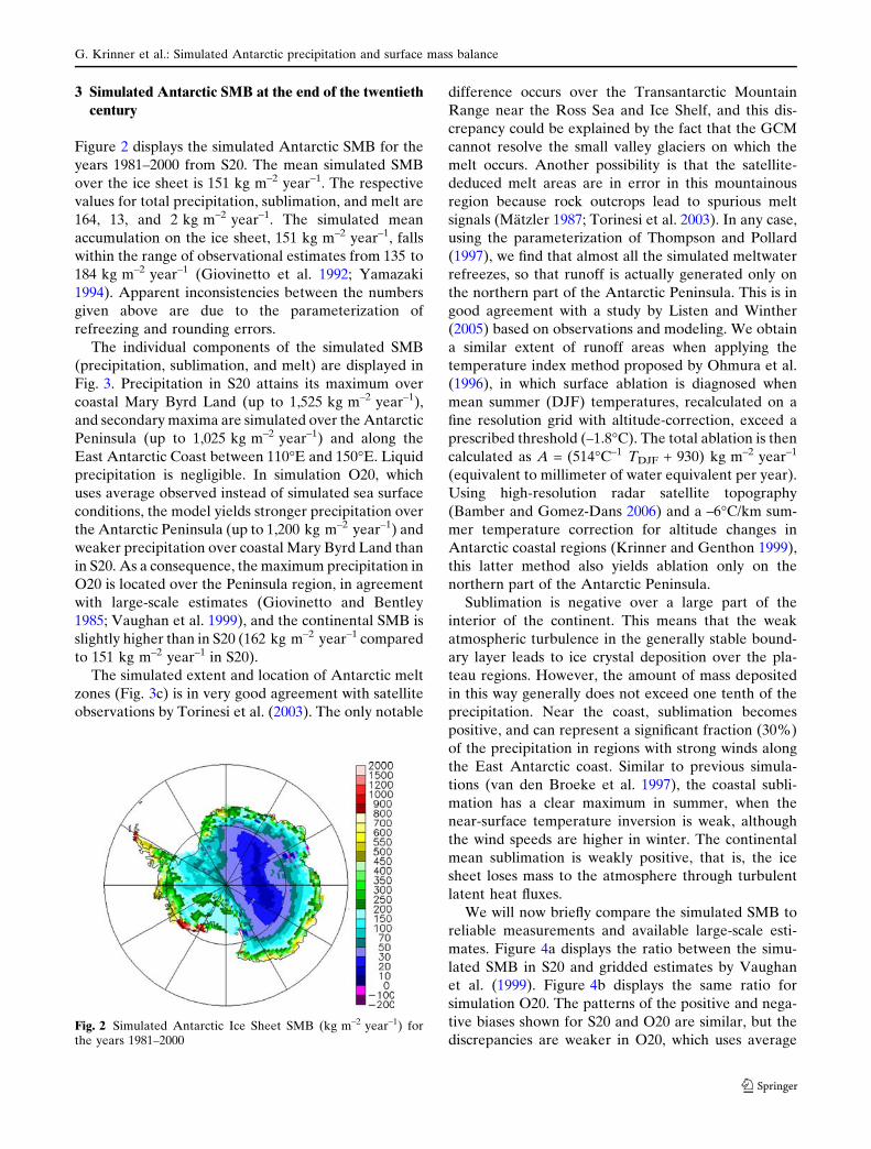
Figure 2 displays the simulated Antarctic SMB for the

years 1981–2000 from S20. The mean simulated SMB

over the ice sheet is 151 kg m–2 year–1. The respective

values for total precipitation, sublimation, and melt are

164, 13, and 2 kg m–2 year–1. The simulated mean

accumulation on the ice sheet, 151 kg m–2 year–1, falls

within the range of observational estimates from 135 to

184 kg m–2 year–1 (Giovinetto et al. 1992; Yamazaki

1994). Apparent inconsistencies between the numbers

given above are due to the parameterization of

refreezing and rounding errors.

The individual components of the simulated SMB

(precipitation, sublimation, and melt) are displayed in

Fig. 3. Precipitation in S20 attains its maximum over

coastal Mary Byrd Land (up to 1,525 kg m–2 year–1),

and secondary maxima are simulated over the Antarctic

Peninsula (up to 1,025 kg m–2 year–1) and along the

East Antarctic Coast between 110�E and 150�E. Liquid

precipitation is negligible. In simulation O20, which

uses average observed instead of simulated sea surface

conditions, the model yields stronger precipitation over

the Antarctic Peninsula (up to 1,200 kg m–2 year–1) and

weaker precipitation over coastal Mary Byrd Land than

in S20. As a consequence, the maximum precipitation in

O20 is located over the Peninsula region, in agreement

with large-scale estimates (Giovinetto and Bentley

1985; Vaughan et al. 1999), and the continental SMB is

slightly higher than in S20 (162 kg m–2 year–1 compared

to 151 kg m–2 year–1 in S20).

The simulated extent and location of Antarctic melt

zones (Fig. 3c) is in very good agreement with satellite

observations by Torinesi et al. (2003). The only notable

difference occurs over the Transantarctic Mountain

Range near the Ross Sea and Ice Shelf, and this dis-

crepancy could be explained by the fact that the GCM

cannot resolve the small valley glaciers on which the

melt occurs. Another possibility is that the satellite-

deduced melt areas are in error in this mountainous

region because rock outcrops lead to spurious melt

signals (Matzler 1987; Torinesi et al. 2003). In any case,

using the parameterization of Thompson and Pollard

(1997), we find that almost all the simulated meltwater

refreezes, so that runoff is actually generated only on

the northern part of the Antarctic Peninsula. This is in

good agreement with a study by Listen and Winther

(2005) based on observations and modeling. We obtain

a similar extent of runoff areas when applying the

temperature index method proposed by Ohmura et al.

(1996), in which surface ablation is diagnosed when

mean summer (DJF) temperatures, recalculated on a

fine resolution grid with altitude-correction, exceed a

prescribed threshold (–1.8�C). The total ablation is then

calculated as A = (514�C–1 TDJF + 930) kg m–2 year–1

(equivalent to millimeter of water equivalent per year).

Using high-resolution radar satellite topography

(Bamber and Gomez-Dans 2006) and a –6�C/km sum-

mer temperature correction for altitude changes in

Antarctic coastal regions (Krinner and Genthon 1999),

this latter method also yields ablation only on the

northern part of the Antarctic Peninsula.

Sublimation is negative over a large part of the

interior of the continent. This means that the weak

atmospheric turbulence in the generally stable bound-

ary layer leads to ice crystal deposition over the pla-

teau regions. However, the amount of mass deposited

in this way generally does not exceed one tenth of the

precipitation. Near the coast, sublimation becomes

positive, and can represent a significant fraction (30%)

of the precipitation in regions with strong winds along

the East Antarctic coast. Similar to previous simula-

tions (van den Broeke et al. 1997), the coastal subli-

mation has a clear maximum in summer, when the

near-surface temperature inversion is weak, although

the wind speeds are higher in winter. The continental

mean sublimation is weakly positive, that is, the ice

sheet loses mass to the atmosphere through turbulent

latent heat fluxes.

We will now briefly compare the simulated SMB to

reliable measurements and available large-scale esti-

mates. Figure 4a displays the ratio between the simu-

lated SMB in S20 and gridded estimates by Vaughan

et al. (1999). Figure 4b displays the same ratio for

simulation O20. The patterns of the positive and nega-

tive biases shown for S20 and O20 are similar, but the

discrepancies are weaker in O20, which uses averageFig. 2 Simulated Antarctic Ice Sheet SMB (kg m–2 year–1) forthe years 1981–2000


123

observed sea surface conditions, than in S20, in which

average simulated sea surface conditions are prescribed.

In both simulations, strong positive biases appear in

coastal Mary Byrd Land. Concerning this particular

region, Genthon and Krinner (2001) showed that this is

a common bias shared by many high-resolution

GCMs and reanalyses. They state that it is possible

that, rather than the models, the gridded SMB esti-

mates of Vaughan et al. (1999) are in error in this

Fig. 3 Individual components of the simulated Antarctic IceSheet SMB (kg m–2 year–1) for the years 1981–2000. a Precip-itation; b sublimation; c melt

Fig. 4 a Ratio between simulated SMB in S20 and estimates byVaughan et al. (1999); b ratio between simulated SMB in O20and estimates by Vaughan et al. (1999); c ratio betweensimulated (S20) and observed SMB in selected Antarcticlocations where reliable observations exist


123

area, because they are based on extrapolations from

SMB measurements in the interior. Regional climate

model simulations by van den Broeke et al. (2006) also

suggest this. A large difference between the errors for

S20 (Fig. 4a) and O20 (Fig. 4b) is the large bias dipole in

West Antarctica in S20. The reason for this problem is

the underestimated intensity of the Amundsen Sea low

pressure zone in S20. As discussed by Genthon et al.

(2005), a weaker Amundsen Sea low leads to increased

precipitation over Mary Byrd Land and reduced pre-

cipitation to the East. These precipitation errors are

absent in simulation O20, which uses observed sea

surface conditions. The model misfit in S20 is thus due to

errors in the sea surface conditions obtained from the

coupled model run. An apparent negative bias both of

S20 and O20 is located in central East Antarctica,

essentially along the ridge of the ice sheet. Here, both

simulations yield lower SMB than the gridded estimates

of Vaughan et al. (1999) suggest. However, as will be

shown in the following, this negative bias in central East

Antarctica does not appear when the model simulations

are compared to selected reliable measurements.

Figure 4c shows the ratio between simulated and

observed SMB for selected locations in Antarctica in

S20. Because of high interannual SMB variability on

small spatial scales (Frezzotti et al. 2004, 2005;

Magand et al. 2004), we selected locations where

data represent at least a decade of SMB (Minikin

et al. 1994; Smith et al. 2002; Pourchet et al. 2003;

Magand et al. 2004; Kaspari et al. 2004; Frezzotti

et al. 2004, 2005) to reduce as much as possible the

effect of small-scale spatial and temporal variability

and thus increase temporal and spatial representa-

tiveness of observed SMB values. This approach

follows the recommendations by the ISMASS Com-

mittee (2004). Additionally, we used observed SMB

data from the Dome F (Watanabe et al. 2003) and

Siple Dome (Taylor et al. 2004) deep drilling sites.

Furthermore, we excluded locations at which the

model topography is in error by more than 300 m.

Surprisingly few data points had to be dropped as a

consequence of this criterion. Few clear and strong

regional biases appear in the figure. In particular, the

model does not show a particular bias in central East

Antarctica, as the comparison to the gridded esti-

mates tended to suggest; on the contrary, the simu-

lated SMB agrees rather well with observed values

from firn cores at the deep drilling sites Dome C,

Dome F, and Vostok. One regional bias seems to

consist in an underestimate of SMB in coastal Wilkes

Land between 110 and 140�E, where the model

simulates less than 66% of the observed values.

Further west, the model seems to overestimate the

SMB, but the bias is not very strong. Around 77�S

and 145�E, a group of three points indicating a

strong overestimate of the SMB is linked to the

presence of wind-glazed surfaces with extremely low

accumulation rates due to sublimation of blowing

snow (Frezzotti et al. 2002, 2004). This is a process

that the model does not represent. Along an axis

from Dome F (39.8�E, 77.3�S) via the South Pole to

Siple Dome (148.8�W, 81.7�S), the model has a ten-

dency to slightly underestimate the SMB. On smaller

spatial scales, however, significant discrepancies exist.

Interestingly, points with large under- and overesti-

mates are often very close to each other. In such

cases, the misfits are largely due to high spatial var-

iability in the data on very short distances (Magand

et al. 2004; Frezzotti et al. 2004, 2005), which cannot

be sufficiently well represented in the model, leading

to spuriously high apparent and localized biases in

Fig. 4c. This is supported by the fact that the

agreement between model and data is generally im-

proved by using only the mean observed SMB of

several data points at places where several data

points correspond to one single model grid point.

For instance, two firn core measurements at

approximately 151.1�E and 74.8�S, at a few hundred

meters from each other, indicate SMBs of 82 and

44 kg m–2 year–1, respectively, with the simulated

SMB (50 kg m–2 year–1) lying between these values.

Taking into consideration these problems linked to

spatial heterogeneity of SMB, we conclude that on

regional scales, SMB is typically represented to

within about 20% of the true value by the GCM,

except in regions where sublimation of blowing

snow has a significant impact on SMB, and except in

regions where the use of simulated sea surface con-

ditions from a coupled model run leads to errors in

the simulated patterns of atmospheric dynamics.

4 Simulated Antarctic SMB at the endof the twenty-first century

Figure 5 displays the simulated Antarctic SMB for the

years 2081–2100. Mean simulated SMB over the ice

sheet is 183 kg m–2 year–1. The respective values for

total precipitation, sublimation, and melt are 199, 15,

and 7 kg m–2 year–1.

Recent observed increases of SMB over central

East Antarctica have been suggested to be a potential

early indicator of anthropogenic climate change

(Mosley-Thompson et al. 1998). Similar to other

simulations of future Antarctic SMB (e.g., Wild et al.

2003), the simulations presented here confirm that


123

future accumulation is indeed greater over most of

the interior of the continent. The physical mechanism

underlying this effect on the continental scale appears

to be the increased moisture holding capacity of the

air at higher temperatures. However, the model also

simulates drying in some regions, such as the interior

of Mary Byrd Land or Wilkes Land (see Fig. 6, which

shows the ratio between the annual mean precipita-

tions of S21 and S20). In spite of regional drying,

though, the continental mean precipitation increases

by 21%. Because the low-lying coastal regions have

much higher mean precipitation rates than the inte-

rior, the continental-mean precipitation increase is

dominated by the coastal areas. The spatially inte-

grated precipitation increase over the grid points

below 1,500 m is twice that of the grid points above

1,500 m, although the total Antarctic surface area

above 1,500 m is almost twice the area below 1,500 m.

Because the precipitation patterns are strongly

determined by topographical features, the continen-

tal-scale pattern of precipitation in S21 is very similar

to that of S20, even in sub-regional details. Rainfall

becomes a significant part (locally up to 30%) of total

annual precipitation at the tip (northernmost 250 km)

of the Antarctic Peninsula. Elsewhere, it generally

remains negligible.

Simulated total snow and ice melt over Antarctica

increases by more than a factor of three (from 2 in

S20 to 7 kg m–2 year–1 in S21), but it still remains

small compared to the total precipitation. Regionally,

though, the increased melt is important, particularly

over the Antarctic Peninsula, where several grid

points with negative SMB exist in S21, due to high

melt rates of up to 800 kg m–2 year–1. As in S20, this

northern part of the Peninsula is the only region where

the melted snow does not refreeze, but is lost as runoff.

Of the continental mean meltwater (7 kg m–2 year–1),

almost 80% is diagnosed to refreeze even at the end

of the twenty-first century. Patterns of latent turbu-

lent surface fluxes in S21 are very similar to that of

S20, with deposition in the interior (but slightly

less than in S20), and sublimation in the coastal

regions.

The Antarctic SMB increase of + 32 kg m–2 year–1

from S20 to S21 corresponds to a net sea level decrease

of 1.2 mm year–1 by the end of the twenty-first century,

compared to the end of the twentieth century.

5 Characteristics of present and future precipitation

5.1 Seasonality

Figure 7 displays the simulated monthly mean total

precipitation and snowfall time series for the Antarctic

Plateau, the east Antarctic coastal area, the Antarctic

Peninsula, and the interior of Mary Byrd Land. The

early winter maximum of simulated east Antarctic

coastal precipitation in S20 is replaced by a broader

winter maximum in S21, but most importantly, the

summer minimum is much less pronounced in S21 than

in S20. Over the plateau regions above 3,000 m alti-

tude, the precipitation increase is more equally dis-

tributed over the year. The present-day autumn

precipitation maximum in the interior of Mary Byrd

Land is replaced by a winter maximum in S21. This

particular feature will be discussed in subsection ‘‘Sea

ice cover, cyclonicity and precipitation’’.

Fig. 5 Simulated Antarctic Ice Sheet SMB (kg m–2 year–1) forthe years 2081–2100, SRESA1B scenario

Fig. 6 Relative annual mean precipitation change on theAntarctic Ice Sheet (S21/S20)


123

5.2 Link between mean circulation, temperature,

and precipitation changes

Obvious features of the prescribed change in annual

mean sea ice concentration from S20 to S21 (Fig. 1b)

are a sea ice concentration increase of Wilkes Land,

and a strong concentration decrease further East, in

the Ross and Amundsen Seas. It is interesting to note

that this pattern is similar to the recent observed

spatial pattern of sea ice edge trends, linked to an

increase of the positive polarity of the Southern

Annular Mode (SAM) as shown by Kwok and Com-

iso (2002). Indeed, the Antarctic Oscillation Index,

defined as the normalized zonal sea level pressure

difference between 40�S and 65�S (Gong and Wang

1999), is higher in S21 than in S20. As stated in the

introduction, this is consistent with many studies of

the impact of enhanced greenhouse gas concentra-

tions on the southern hemisphere circulation patterns

(Fyfe et al. 1999; Kushner et al. 2001; Stone et al.

2001; Cai et al. 2003; Marshall et al. 2004). In a

manner that is coherent with the impact on sea ice,

positive phases of the SAM lead to a warming

over the Antarctic Peninsula and a cooling (or a

weaker warming in a global change context) over East

Antarctica (Kwok and Comiso 2002). Precipitation in

high latitudes is often limited by the low water

holding capacity of cold air. The precipitation reduc-

tion in Wilkes Land simulated by LMDZ4 is there-

fore not too surprising. Of course, modifications in the

mean state of the Southern Annular Mode could also

influence factors other than air temperatures, such as

moisture source regions, but here we focus on the

link between temperature and precipitation. In this

respect, it is worth noting that the relative precipitation

change shown in Fig. 6 shows some striking similari-

ties to the relative precipitation change simulated by

the ECHAM4 model (Huybrechts et al. 2004).

We will now analyse the link between precipitation

and temperature changes in some more detail. Fol-

lowing the water holding capacity argument, one can

expect a roughly exponential link between tempera-

ture and precipitation changes over Antarctica (e.g.,

Robin 1977). Strictly speaking, the pertinent tempera-

ture in this case is not the annual mean temperature,

but the temperature during the months when precipi-

tation preferentially falls. Following Krinner et al.

(1997a) and Krinner and Werner (2003), we therefore

introduce the precipitation-weighted temperature Tpr,

defined as

Fig. 7 Simulated monthly mean precipitation (kg m–2 month-1)for the periods 1981–2000 (black) and 2081–2100 (red), fordifferent Antarctic regions. Full lines: Total precipitation; dashedlines: snowfall. Total precipitation and snowfall are almostindistinguishable except on the Peninsula. The Antarctic Plateauincludes all grid points above 3,000 m altitude. Coastal East

Antarctica includes all grid points below 2,000 m altitude, atlongitudes between 30�W and 180�E, and north of 78�S in orderto exclude shelf areas. The Peninsula region is defined as the areanorth of 75�S, at longitudes between 80�W and 50�W. Theinterior of Mary Byrd Land is the region between 80 and 85�south and between 150 and 120� west


123

Tpr¼XðTiPiÞ=

XPi

where Ti and Pi indicate monthly mean surface air

temperature and precipitation, and the sums are cal-

culated over the 12 months of the simulated mean

annual cycle. Figure 8 displays the simulated temper-

ature changes (S21–S20) and precipitation-weighted

temperature changes (S21–S20). On subcontinental

scales, no link is apparent between the annual mean

temperature change (Fig. 8a) and the relative precipi-

tation change (Fig. 6). Conversely, there is a fairly

clear, though less than perfect, match between the

relative precipitation change and the change in pre-

cipitation-weighted temperature (Fig. 8b). In regions

where Tpr increases only slightly, precipitation does not

increase or even decreases, while strong precipitation

increases tend to be linked to strong Tpr increases. This

is interesting, as it indicates that the link between

precipitation and temperature changes is not as simple

as often assumed in ice core studies, in particular in ice

core dating exercises, where a fixed relationship be-

tween mean annual temperature and accumulation,

and changes thereof, is commonly assumed (e.g., Par-

renin et al. 2004). However, this issue is beyond the

scope of the present study. In any case, the fact that the

patterns in Figs. 6 and 8b do not match perfectly

indicates that other processes also influence the pre-

cipitation changes in Antarctica. These will be analy-

sed in the following.

5.3 Sea ice cover, cyclonicity and precipitation

Watkins and Simmonds (1995) have shown that an

intimate synoptic connection exists between sea ice

and cyclone behaviour, which gives rise to the general

relationship between Antarctic Sea ice concentration

and cyclonicity reported by Simmonds and Wu (1993).

Following these findings, the simulated changes in cy-

clonic system density (Fig. 9) are consistent with the

sea ice concentration changes displayed in Fig. 1b. Off

Wilkes Land, the increased sea ice concentration re-

duces the local moisture source and weakens the cy-

clonic systems, both effects leading to reduced

precipitation shown in Fig. 6, and thus adding to the

effects of the mean circulation and temperature chan-

ges discussed in the previous section.

Again in agreement with the findings of Simmonds

and Wu (1993), decreased sea ice concentration along

the Antarctic Peninsula in the Weddell Sea in S21

leads to increased lee cyclogenesis, and thus to in-

creased system density, in this area. This strengthened

cyclonic circulation over the Weddell Sea induces a

strong precipitation increase on Coates Land in S21,

contrary to the region south of the Filchner/Ronne Ice

Shelf, which is more exposed to outflow of cold air

from the East Antarctic Plateau.

The situation is different in the interior of Mary

Byrd Land, where precipitation decreases in S21

compared to S20 (Fig. 6). The precipitation reduction

is essentially due to a substantial precipitation reduc-

tion during the autumn months, particularly in March,

as can be seen in Fig. 7d. For the present, the model

simulates a clear precipitation maximum during these

months in the interior of Mary Byrd Land, while this

maximum disappears in S21. This is due to sea level

pressure differences between S21 and S20 in the

Amundsen Sea off Mary Byrd Land, as can be seen in

Fig. 8 Link between temperature and precipitation changes onthe Antarctic Ice Sheet. a Simulated annual mean surface airtemperature change (S21-S20, �C); b simulated change of annualmean precipitation-weighted surface air temperature (S21-S20,�C)


123

Fig. 10. The decrease in autumn sea level pressure over

the Amundsen Sea in S21, linked to the sea-ice con-

centration decrease shown in Fig. 1b, strengthens the

flow of cold and dry air masses from the top of the

West Antarctic Ice Sheet across the interior of Mary

Byrd Land. Closer to the coast, the increased annual

mean cyclonic activity (Fig. 9) does induce a strong

annual mean precipitation increase. In this context, it is

noteworthy that a maximum of climate variability

exists in the Amundsen and Bellingshausen Seas, due

to the asymmetric nature of the orography in Antarc-

tica (Lachlan-Cope et al. 2001a). In some cases, this

variability seems to be excited by ENSO (e.g.,

Genthon and Cosme 2003; Fogt and Bromwich 2006),

but the observed variability, which climate models tend

to reproduce fairly correctly, ‘‘has a white spectrum

consistent with random forcing by weather events and

a decoupling from oceanic integration’’ (Connolley

1997). Given, in addition, that the prescribed sea sur-

face conditions in our simulations have no interannual

variability, and that no clear El-Nino type signal exists

in either the prescribed tropical mean SST changes in

our model runs or in the simulated sea level pressure

pattern changes over the South Pacific, a modified

ENSO forcing can be ruled out as cause for the pre-

cipitation changes in West Antarctica simulated in this

model.

5.4 Intensity of individual precipitation events

Additional insight into the characteristics of precipi-

tation events can be gained by analyzing the intensity

of individual precipitation events. Figure 11 displays

the number of days per year with daily precipitation

exceeding five times the mean daily precipitation for

the corresponding simulation (‘‘NP5’’ in the following).

The threshold value for a precipitation event to be

classified as ‘‘intense’’ therefore depends on the mean

precipitation at each point, and varies between S20 and

S21. NP5 is tightly linked to the model topography. For

the present (Fig. 11a), NP5 attains minimum values of

only 4 days per year on the ridge of the East Antarctic

Plateau, and regional minima systematically over other

ice sheet domes and ridges, and on mountain chains

(e.g., on the Peninsula). Maximum values of NP5 are

attained in coastal East Antarctica, coastal Mary Byrd

Land, and on the flat major shelves (Ross and Filchner/

Ronne). In these areas, daily precipitation exceeds five

Fig. 9 Simulated mean density of cyclonic systems (10–3/(�lat)2).a 1981–2000 (S20); b 2081–2100 (S21)

Fig. 10 Simulated sea-level pressure difference (hPa) betweenS21 and S20 in march


123

times the mean daily precipitation on 20 days or more,

indicating that frequent and strong cyclones off the

coast bring the bulk of the annual total precipitation, as

indicated by observations (Bromwich et al. 1988). In

agreement with measurements in the interior of

Dronning Maud Land (around 75�S, 0�E) by Reijmer

et al. (2002), simulated NP5 is fairly high in this region.

Conversely, on the plateau regions, and particularly on

the ridges and domes, precipitation is more evenly

distributed in time. This does not mean that there

cannot be a distinct seasonality (see Fig. 7), but it

indicates that precipitation tends to fall in relatively

smaller amounts and on more frequent occasions.

Because the precipitation amounts on the central

Antarctic Plateau are so tiny, reliable measurements of

the intensity of particular events do not exist. Fairly

frequent and light clear sky precipitation (‘‘diamond

dust’’) is thought to deliver the major part of total

precipitation in the remote interior (e.g., Bromwich

1988; Lachlan-Cope et al. 2001b), but blocking-high

activity in the Southern Ocean can occasionally cause

oceanic air masses to intrude far into the interior and

lead to significant precipitation, as for example during

the 2001/2002 summer season at Dome C (Massom

et al. 2004). The low values of NP5 over the Antarctic

Peninsula, however, are linked to the high frequency of

cyclonic perturbations around this area (Fig. 9a),

leading to high annual mean precipitation (Fig. 3a)

delivered by many more or less equally strong precip-

itation events, and is consistent with observations

(Turner et al. 1995; Russell et al. 2004). The pattern of

NP5 for simulation S21 (not shown) is very similar to

that for S20. The relative change of NP5 from S20 to

S21 (Fig. 11b) indicates that the number of relatively

strong precipitation events near the ice sheet domes

and ridges, in particular in central East Antarctica,

increases. Because the mean precipitation increases

from S20 to S21, this also means that the frequency of

strong precipitation events in the interior would be

found to increase if, in the definition of what such an

intense event is, the same numeric value of the

threshold was used in S20 and S21. This indicates an

increased frequency of intrusions of moist marine air,

in spite of a lower future cyclonic system density.

These apparently conflicting findings can be reconciled

by recognizing that the intensity of the simulated

cyclonic systems off the East Antarctic Coast, mea-

sured as the depth of the cyclonic depression in hPa of

sea level pressure, increases from about 10 hPa in S20

to about 12 hPa in S21 (not shown). In other words,

although the model suggests that there will be less

cyclones off the East Antarctic coast in the future, the

remaining cyclones will carry oceanic moisture further

inland.

6 Concluding summary and discussion

The present-day Antarctic surface mass balance, as

simulated by the LMDZ4 AGCM at a resolution of

about 60 km over large parts of the continent, is in

good agreement with continental-scale estimates. On

regional scales, biases of about 20% appear when

observed sea surface conditions are prescribed as

boundary condition. The use of sea surface conditions

from a coupled model run regionally induces larger

biases. Such problems could be avoided by construct-

ing sea surface boundary conditions for the twenty-first

Fig. 11 Number of days with precipitation exceeding five timesthe annual daily mean (NP5). a Present day (S20); b relativechange from the end of the twentieth to the end of the twenty-first century (S21-S20, in percent)


123

century with an anomaly method using present-day

observed sea surface conditions and coupled model

anomalies. However, such anomaly methods can be

problematic because the different aspects of the sim-

ulated climate change (such as the amplitude of the

latitudinal shift of the sea ice edge, total sea ice area

variations, sea surface temperature change, and re-

gional differences in these changes) usually cannot all

be reproduced in a faithful and meaningful way in the

constructed forcing field. In this study, we therefore

chose to use the sea surface conditions from the cou-

pled IPCC model run directly. On local scales, the

SMB biases can be rather large, but we suspect that

high fine scale spatial variability, which cannot be

captured by the model, leads to low representativeness

of many point measurements. In some regions, model-

data misfits seem to be due to the missing representa-

tion of the sublimation of blowing snow. This process

should be taken into account in future versions of the

model. The results we obtain indicate that realistic

estimates of Antarctic surface melt and the induced

mass loss can be obtained by using the surface melt

that is directly simulated by the model and applying a

parameterization of refreezing of surface water. This

approach leads to a very low estimated mass loss

through surface melt, both in present-day and future

(end of the twenty-first century) conditions. The spatial

resolution used in these simulations seems sufficient for

a reasonable assessment of the continental and re-

gional scale surface mass balance in Antarctica. It re-

mains to be seen whether this direct approach at

similar resolution can be applied to Greenland, where

melt on the margins of the ice sheet is much more

intense.

The model suggests an Antarctic surface mass

balance (SMB) increase of + 32 kg m–2 year–1 from

within the 100 years from 1981–2000 to 2081–2100,

corresponding to a net sea level decrease of

1.2 mm year–1 by the end of the twenty-first century.

This is the same as the value obtained by Wild et al.

(2003) with the ECHAM4 GCM at about 100 km

horizontal resolution. However, the numbers cannot

be compared strictly because Wild et al. (2003) sim-

ulate the climate change between the present and the

approximate time of CO2 concentration doubling with

respect to pre-industrial values (which occurs around

2060 in the SRES A1B scenario used as a basis for

our simulations). In a study using a regional climate

model at 55 km resolution, van Lipzig et al. (2002)

prescribed a 2�C temperature increase at the sea

surface and the lateral boundaries around Antarctica,

while keeping constant the relative humidity at the

lateral boundaries. This increased humidity transport

towards the Antarctic leads to a 30% increase of the

continental-scale SMB. The experiment by van Lipzig

et al. (2002) is of course not easily compared with

ours, but given the approximate temperature increase

of about 3�C in our simulations, and a concomitant

SMB (and precipitation) increase of about 21%, it

appears that the SMB sensitivity obtained by van

Lipzig et al. (2002) is clearly stronger than what is

suggested by our model. It is also stronger than the

SMB sensitivities reported by Huybrechts et al. (2004)

for the ECHAM4 and HadAM3H models, because

these are close to the value obtained with LMDZ4. In

this respect, it is noteworthy that the 2�C warming

prescribed by van Lipzig et al. (2002) at the lateral

boundaries of their model, typically around 55�S,

roughly corresponds to the tropospheric temperature

increase simulated by LMDZ4 in this region, the

prescribed sea surface temperature increase in the

region being somewhat weaker.

If we suppose that the change in SMB simulated by

LMDZ4 is linear in the next 100 years, this SMB

increase would lead to a cumulated sea level decrease

of about 6 cm. However, it is clear that changes in

glacier dynamics, particularly in West Antarctic ice

streams, might have important impacts on future sea

level changes. These changes in glacier dynamics

might be caused by an increased surface melt in low-

lying areas of Antarctica, although the model indi-

cates that the overwhelming part of the meltwater

will refreeze also at the end of the twenty-first

century. Future surface mass balance changes in

Antarctica can thus essentially be traced back to

precipitation changes. Although there is a continen-

tal-scale increase of precipitation going along with a

continental-scale warming, the link between precipi-

tation and temperature change is more complicated

than often assumed. Changes in atmospheric dynam-

ics, largely influenced by sea-ice changes, modulate

this relationship on regional scales. Moreover, the

seasonality of precipitation and temperature, and

changes thereof, are important parameters that have

to be taken into account in the analyses of this rela-

tionship. In the interior of Antarctica, precipitation

increases roughly equally at all seasons, while in

coastal regions, the signal is more complicated and

spatially variable. The simulated increase (decrease)

of cyclonic system density in West (East) Antarctica

seems to be an important factor in these changes.

In the interior of the continent, intrusion of marine

air masses pushed by powerful coastal weather sys-

tems becomes more frequent, because the mean

intensity of coastal cyclones off the East Antarctic

coast increases.


123

Acknowledgments This work was financed by the French pro-grams ACI C3 et MC2 and the European integrated projectENSEMBLES. The simulations were carried out on the Miragecomputer platform in Grenoble. Additional computer resourcesat IDRIS are acknowledged. In Wilkes and Victoria Land sec-tors, most of observed SMB data were obtained from recentresearch carried out in the framework of the Project on Glaci-ology of the PNRA-MIUR and financially supported by PNRAconsortium through collaboration with ENEA Roma, and sup-ported by the French Polar Institute (IPEV). This last work is aFrench–Italian contribution to the ITASE Project. The authorsthank two anonymous referees for useful comments.

References

Alexeev VA, Langen PL, Bates JR (2005) Polar amplification ofsurface warming on an aquaplanet in ‘‘ghost forcing’’experiments without sea ice feedbacks. Clim Dyn 24:655–666

de Angelis H, Skvarca P (2003) Glacier surge after ice shelfcollapse. Science 299:1560–1562

Bamber JL, Gomez-Dans JL (2006) The accuracy of digitalelevation models of the Antarctic continent. Earth Plane-tary Sci Lett 237:516–523

Bromwich D (1988) Snowfall in high southern latitudes. RevGeophys 26:149–168

Cai W, Whetton PH, Karoly DJ (2003) The response of theAntarctic oscillation to increasing and stabilized atmo-spheric CO2. J Clim 16:1525–1538

Connolley WM (1997) Variability in annual mean circulation insouthern high latitudes. Clim Dyn 13:745–756

Cook AJ, Fox AJ, Vaughan DG, Ferrigno JG (2005) Retreatingglacier fronts on the Antarctic Peninsula over the past half-century. Science 308:541–544

Cuffey K, Clow GD, Alley RB, Stuiver M, Waddington E,Saltus R (1997) Large Arctic temperature change at theWisconsin-Holocene deglacial transition. Science 270:455–458

Davis CH, Li Y, McConnell JR, Frey MM, Hanna E (2005)Snowfall-driven growth in East Antarctic Ice Sheet miti-gates recent sea-level rise. Science 308:1877–1878

Domack E, Duran D, Leenter A, Ishman S, Doane S, McCallumS, Amblas D, Ring J, Gilbert R, Prentice M (2005) Stabilityof the Larsen B ice shelf on the Antarctic Peninsula duringthe Holocene epoch. Nature 436:681–685

Doran PT, Priscu JC, Lyons WB, Walsh JE, Fountain AG,McKnight DM, Moorhead DL, Virginia RA, Wall DH,Clow GD, Fritsen CH, McKay CP, Parsons AN (2002)Antarctic climate cooling and terrestrial ecosystem re-sponse. Nature 415:517–520

Dufresne JL, Quaas J, Boucher O, Denvil S, Fairhead L (2005)Contrasts in the effects on climate of anthropogenic sulfateaerosols between the 20th and the 21st century. GeophysRes Lett 32:L21703. DOI 10.1029/2005GL023619

Ekaykin AA, Lipenkov VY, Kuzmina IN, Petit JR, Masson-Delmotte V Johnsen SJ (2004) The changes in isotopecomposition and accumulation of snow at Vostok stationover the past 200 years. Ann Glaciol 39:569–575

EPICA Project Members (2004) Eight glacial cycles from anAntarctic ice core. Nature 429:623–628

Fogt RL, Bromwich DH (2006) Decadal variability of the ENSOteleconnection to the high latitude South Pacific governedby coupling with the Southern Annular Mode. J Clim19:979–997

Forster PM, Taylor KE (2006) Climate forcings and climatesensitivities diagnosed from coupled climate model inte-grations. J Clim (in press)

Frezzotti M, Gandolfi S, La Marca F, Urbini S (2002) Snowdunes and glazed surfaces in Antarctica: new field and re-mote-sensing data. Ann Glaciol 34:81–88

Frezzotti M, Pourchet M, Flora O,Gandolfi S, Gay M, Urbini S,Vincent C, Becagli S, Gragnani R, Proposito M, Severi M,Traversi R, Udisti R, Fily M (2004) New estimations ofprecipitation and surface sublimation in East Antarcticafrom snow accumulation measurements. Clim Dyn 23:803–813

Frezzotti M, Pourchet M, Flora O,Gandolfi S, Gay M, Urbini S,Vincent C, Becagli S, Gragnani R, Proposito M, Severi M,Traversi R, Udisti R, Fily M (2005) Spatial and temporalvariability of snow accumulation in East Antarctica fromtraverse data. J Glaciol 172:113–124

Fyfe JC, Boer GJ, Flato GM (1999) The Arctic and Antarcticoscillations and their projected changes under globalwarming. Geophys Res Lett 26:1601–1604

Gallee H, Guyomarc’h G, Brun E (2001) Impact of snow drift onthe Antarctic Ice Sheet Surface Mass Balance: possiblesensitivity to snow-surface properties. Boundary LayerMeteorol 99:1–19

Genthon C, Kaspari S, Mayewski PA (2005) Interannual vari-ability of the surface mass balance of West Antarctica fromITASE cores and ERA40 reanalyses, 1958–2000. Clim Dyn24:759–770

Genthon C, Krinner G (2001) Antarctic surface mass balanceand systematic biases in general circulation models. J Geo-phys Res 106:20653–20664

Genthon C, Cosme E (2003) Intermittent signature of ENSO inWest-Antarctic precipitation. Geophys Res Lett 30: 2081.DOI 10.1029/2003GL018280

Giovinetto MB, Bentley CR (1985) Surface balance in icedrainage systems of Antarctica. Antarct J US 20:6–13

Giovinetto MB, Bromwich DH, Wendler G (1992) Atmosphericnet transport of water vapor and latent heat across 70�S. JGeophys Res 97:917–930

Gillet NP, Thompson DWJ (2003) Simulation of recent southernhemisphere climate change. Science 302:273–275

Gong D, Wang S (1999) Definition of Antarctic oscillation index.Geophys Res Lett 26:459–462

Holland MM, Bitz CM (2003) Polar amplification of climatechange in coupled models. Clim Dyn 21:221–232

Hourdin F, Musat I, Bony S, Braconnot P, Codron F, DufresneJL, Fairhead L, Filiberti MA, Friedlingstein P, GrandpeixJY, Krinner G, Le Van P, Li ZX, Lott F (2006) The LMDZ4general circulation model: climate performance and sensi-tivity to parametrized physics with emphasis on tropicalconvection. Clim Dyn (in press)

Huybrechts P, Gregory J, Janssens I, Wild M (2004) ModellingAntarctic and Greenland volume changes during the 20thand 21st centuries forced by GCM time slice integrations.Glob Planet Change 42:83–105

ISMASS Committee (2004) Recommendations for the collectionand synthesis of Antarctic Ice Sheet mass balance data.Glob Planet Change 42:1–15

Kaspari S, Mayewski PA, Dixon DA, Spikes VB, Sneed SB,Handley MJ, Hamilton GS (2004) Climate variability inWest Antarctica derived from annual accumulation-raterecords from ITASE firn/ice cores. Ann Glaciol 39:585–594

Krinner G, Genthon C (1997) The Antarctic surface mass bal-ance in a stretched grid general circulation model. AnnGlaciol 25:73–78


123

Krinner G, Genthon C (1998) GCM simulations of the last gla-cial maximum surface climate of Greenland and Antarctica.Clim Dyn 14:741–758

Krinner G, Genthon C (1999) Altitude dependence of the icesheet surface climate. Geophys Res Lett 26:2227–2230

Krinner G, Werner M (2003) Impact of precipitation seasonalitychanges on isotopic signals in polar ice cores: a multi-modelanalysis. Earth Planet Sci Lett 216:525–538

Krinner G, Genthon C, Jouzel J (1997a) GCM analysis of localinfluences on ice core d signals. Geophys Res Lett 24:2825–2828

Krinner G, Genthon C, Li ZX, Le Van P (1997b) Studies of theAntarctic climate with a stretched grid GCM. J GeophysRes 102:13731–13745

Krinner G, Mangerud J, Jakobsson M, Crucifix M, Ritz C,Svendsen JI (2004) Enhanced ice sheet growth in Eurasiaowing to adjacent ice-dammed lakes. Nature 427:429–432

Kushner PJ, Held IM, Delworth TL (2001) Southern hemisphereatmospheric circulation response to global warming. J Clim14:2238–2249

Kwok R, Comiso JC (2002) Spatial patterns of variability inAntarctic surface temperature—connections to the southernhemisphere Annular Mode and the Southern Oscillation.Geophys Res Lett 29: 50. DOI 10.1029/2002GL015415

Lachlan-Cope T, Connolley W, Turner J (2001a) The role ofnon-axisymmetric Antarctic orography in forcing the ob-served pattern of variability of the Antarctic climate. Geo-phy Res Lett 28:4111–4114

Lachlan-Cope T, Ladkin R, Turner J, Davison P (2001b)Observations of cloud and precipitation particles on theAvery Plateau, Antarctic Peninsula. Antarct Sci 13:339–348

van Lipzig NPM, van Meijgaard E, Oerlemans J (2002) Tem-perature sensitivity of the Antarctic Surface Mass Balancein a regional atmospheric climate model. J Clim 15:2758–2774

Listen GE, Winther J-G (2005) Antarctic surface and subsurfacesnow and ice melt fluxes. J Clim 18:1469–1481

Magand M, Frezzotti M, Pourchet M, Stenni B, Genoni L, Fily M(2004). Climate variability along latitudinal and longitudinaltransects in East Antarctica. Ann Glaciol 39:351–358

Marshall GJ, Scott PA, Turner J, Connolley WM, King JC,Lachlan-Cope TA (2004) Causes of exceptional atmosphericcirculation changes in the southern hemisphere. GeophysRes Lett 31: L14205. DOI 10.1029/2004GL019952

Marti O, Braconnot P, Bellier J, Benshila R, Bony S, BrockmannP, Cadule P, Caubel A, Denvil S, Dufresne JL, Fairhead L,Filiberti MA, Foujols MA, Fichefet T, Friedlingstein P,Grandpeix JY, Hourdin F, Krinner G, Levy C, Madec G,Musat I, de Noblet-Ducoudre N, Polcher J, Talandier C(2005). The new IPSL climate system model: IPSL-CM4.Note du Pole de Modelisation n. 26, IPSL, ISSN 1288–1619.http://www.dods.ipsl.jussieu.fr/omamce/IPSLCM4/Doc-IPSLCM4/

Massom RA, Pook MJ, Comiso JC, Adams N, Turner J, Lach-lan-Cope T, Gibson TT (2004) Precipitation over the inte-rior East Antarctic Ice Sheet related to midlatitudeblocking-high activity. J Clim 17:1914–1928

Masson-Delmotte V, Kageyama M, Braconnot P, Charbit S,Krinner G, Ritz C, Guilyardi E, Jouzel J, Abe-Ouchi A,Crucifix M, Gladstone RM, Hewitt CD, Kitoh A, LegrandeA, Marti O, Merkel U, Motoi T, Ohgaito R, Otto-BliesnerB, Peltier WR, Ross I, Valdez PJ, Vettoretti G, Weber SL,Wolk F (2006) Past and future polar amplification of climatechange: climate model intercomparisons and ice-core con-straints. Clim Dyn 26:513–529

Matzler C (1987) Applications of the interaction of microwaveswith the natural snow cover. Remote Sens Rev 2:259–387

Miller L, Douglas BC (2004) Mass and volume contributionsto twentieth-century global sea level rise. Nature 428:406–409

Minikin A, Wagenbach D, Graf W, Kipfstuhl S (1994) Spatialand temporal variations of the snow chemistry at the centralFilchner Ronne Ice Shelf, Antarctica. Ann Glaciol 20:440–447

Monaghan AJ, Bromwich DH, Wang S-H (2006) Recent trendsin Antarctic snow accumulation from Polar MM5. PhilosTrans R Soc Lond A 364:1683–1708

Mosley-Thompson E, Paskievitch JF, Gow AJ, Thompson LG(1998) Late 20th century increase in South Pole snowaccumulation. J Geophys Res 104:3877–3886

Moritz RE, Bitz CM, Steig EJ (2002) Dynamics of recent climatechange in the Arctic. Science 297:1497–1502

Murray R, Simmonds I (1991) A numerical scheme for trackingcyclone centres from digital data. Part I development andoperation of the scheme. Aust Meteorol Mag 39:167–180

Noone D, Simmonds I (1998) Implications for the interpretationof ice-core isotope data from analysis of modelled Antarcticprecipitation. Ann Glaciol 27:398–402

Noone D, Turner J, Mulvaney R (1999) Atmospheric signals andcharacteristics of accumulation in Dronning Maud Land,Antarctica. J Geophys Res 104:19191–19211

Ohmura A, Wild M, Bengtsson L (1996) A possible change inmass balance of Greenland and Antarctic ice sheets in thecoming century. J Clim 9:2124–2135

Parrenin F, Remy F, Ritz C, Siegert MJ, Jouzel J (2004) Newmodeling of the Vostok ice flow line and implication for theglaciological chronology of the Vostok ice core. J GeophysRes 109:D20102. DOI 10.1029/2004JD004561

Pfeffer WT, Meier MF, Illangasekare HT (1991) Retention ofGreenland runoff by refreezing: implications for projectedfuture sea level change. J Geophys Res 96:22117–22124

Phillpot HR, Zillman JW (1970) The surface temperatureinversion over the Antarctic continent. J Geophys Res75:4161–4169

Pourchet M, Magand O, Frezzotti M, Ekaykin A, Winther JG(2003). Radionuclides deposition over Antarctica. J EnvironRadioactivity 68:137–158

Reijmer CH, van den Broeke MR, Schelle MP (2002) Air parceltrajectories and snowfall related to five deep drilling loca-tions in Antarctica based on the ERA-15 dataset. J Clim15:1957–1968

Robin G (1977) Ice cores and climatic changes. Philos Trans RSoc Lond B 280:143–168

Russell A, McGregor GR, Marshall GJ (2004) An examinationof the precipitation delivery mechanisms for Dolleman Is-land, eastern Antarctic Peninsula. Tellus 56A:501–513

Shindell DT, Schmidt GA (2004) Southern hemisphere climateresponse to ozone changes and greenhouse gas increases.Geophys Res Lett 31:L18209

Simmonds I (1985) Analysis of the ‘‘Spinup’’ of a general cir-culation model. J Geophys Res 90:5637–5660

Simmonds I (2003) Modes of atmospheric variability over theSouthern Ocean. J Geophys Res 108: 8078. DOI 10.1029/2000JC000542

Simmonds I, Keay K (2000) Mean southern hemisphere extra-tropical cyclone behaviour in the 40-year NCEP-NCARanalysis. J Clim 13:873–885

Simmonds I, Murray RJ (1999) Southern extratropical cyclonebehaviour in ECMWF analyses during the FROST SpecialObserving Periods. Weather Forecast 14:878–891


123

Simmonds I, Wu X (1993) Cyclone behaviour response tochanges in winter southern hemisphere sea-ice concentra-tion. Q J R Meteorol Soc 119:1121–1148

Smith BT, Van Ommen TD, Morgan VI (2002) Distribution ofoxygen isotope ratios and snow accumulation rates in Wil-helm II Land, East Antarctica. Ann Glaciol 35:107–110

Stone DA, Weaver AJ, Stouffer RJ (2001) Projection of climatechange onto modes of atmospheric variability. J Clim14:3551–3565

Taylor KC, White JWC, Severinghaus JP, Brook EJ, MayewskiPA, Alley RB, Steig EJ, Spencer MK, Meyerson E, MeeseDA, Lamorey GW, Grachev A, Gow AJ, Barnett BA(2004) Abrupt climate change around 22 ka on the SipleCoast of Antarctica. Q Sci Rev 23:7–15

Thomas R, Rignot E, Casassa G, Kanagaratnam P, Acuna C,Akins T, Brecher H, Frederick E, Gogineni P, Krabill W,Manizade S, Ramamoorthy H, Rivera A, Russell R, Sonn-tag J, Swift R, Yungel J, Zwally J (2004) Accelerated sea-level rise from West Antarctica. Science 306:255–258

Thompson DWJ, Solomon S (2002) Interpretation of recentsouthern hemisphere climate change. Science 296:895–899

Thompson SL, Pollard D (1997) Greenland and Antarctic massbalances for present and doubled atmospheric CO2 from theGENESIS Version-2 Global Climate Model. J Clim 10:871–900

Torinesi O, Fily M, Genthon C (2003) Variability and trends ofthe summer melt period of Antarctic ice margins since 1980from microwave sensors. J Clim 16:1047–1060

Turner J, Lachlan-Cope TA, Thomas JP, Colwell S (1995) Thesynoptic origins of precipitation over the Antarctic Penin-sula. Antarct Sci 7:327–337

Turner J, Harangozo SA, Marshall GJ, King JC, Colwell SR(2002) Anomalous atmospheric circulation over the Wed-dell Sea, Antarctica during the austral summer of 2001/2resulting in extreme sea ice conditions. Geophys Res Lett29:2160. DOI 10.1029/2002GL015565

Turner J, Lachlan-Cope TA, Colwell S, Marshall GJ, ConnolleyWM (2006) Significant warming of the Antarctic wintertroposphere. Science 311:1914–1917

van de Berg WJ, van den Broeke MR, Reijmer CH (2006)Reassessment of the Antarctic surface mass balance usingcalibrated input of a regional atmospheric climate model. JGeophys Res 111:D11104. DOI: 10.1029/2005JD006495

van den Broeke MR (1997) Spatial and temporal variation ofsublimation on Antarctica: results of a high-resolution gen-eral circulation model. J Geophys Res 102:29765–29777

van den Broeke MR (2005) Strong surface melting precededcollapse of Antarctic peninsula ice shelf. Geophys Res Lett32:L12815

van den Broeke MR, van der Berg WJ, van Meijgaard E (2006)Snowfall in coastal West Antarctica much greater thanpreviously assumed. Geophys Res Lett 33:L02505

Vaughan DG, Bamber JL, Giovinetto M, Russell J, Cooper APR(1999) Reassessment of net surface mass balance in Ant-arctica. J Clim 12:933–946

Vaughan DG, Marshall GJ, Connolley WM, Parkinson C, Mul-vaney R, Hogson DA, King JC, Pudsey CJ, Turner J (2003)Recent rapid regional climate warming on the AntarcticPeninsula. Clim Change 60:243–274

Watanabe O, Jouzel J, Johnsen S, Parrenin P, Shoji H, YoshidaN (2003) Homogeneous climate variability across EastAntarctica over the past three cycles. Nature 422:509–512

Watkins AB, Simmonds I (1995) Sensitivity of numerical prog-noses to Antarctic sea ice distribution. J Geophys Res100:22681–22696

Wild M, Calanca P, Scherrer S, Ohmura A (2003) Effects ofpolar ice sheets on global sea level in high-resolutiongreenhouse scenarios. J Geophys Res 108:4165

Yamazaki K (1994) Moisture budget in the Antarctic atmo-sphere. In: Jones HG, Davies TD, Ohmura A, Morris EM(eds) Snow and ice covers: interactions with the atmosphereand ecosystems. IAHS Publication No. 233, IAHS Press, pp61–67

Zwally HJ, Abdalati W, Herring T, Larson K, Saba J, Steffen K(2002) Surface melt-induced acceleration of Greenland Ice-Sheet flow. Science 297:218–222


123

Documents

Simulated Antarctic precipitation and surface mass balance