Simple Power Analysis Applied to

Nonlinear Feedback Shift Registers

Abdulah Abdulah Zadeh and H. M. Heys

Electrical and Computer Engineering

Memorial University of Newfoundland

{a.zadeh,hheys}@mun.ca

Abstract

Linear feedback shift registers (LFSRs) and nonlinear feedback shift registers (NLF-

SRs) are major components of stream ciphers. It has been shown that, under cer-

tain idealized assumptions, LFSRs and LFSR-based stream ciphers are susceptible

to cryptanalysis using simple power analysis (SPA). In this paper, we show that

simple power analysis can be practically applied to a CMOS digital hardware cir-

cuit to determine the bit values of an NLFSR and SPA therefore has applicability

to NLFSR-based stream ciphers. A new approach is used with the cryptanalyst

collecting power consumption information from the system on both edges (trigger-

ing and non-triggering) of the clock in the digital hardware circuit. The method is

applied using simulated power measurements from an 80-bit NLFSR targeted to a

180 nm CMOS implementation. To overcome inaccuracies associated with mapping

power measurements to the cipher data, we offer novel analytical techniques which

help the analysis to find the bit values of the NLFSR. Using the obtained results,

we analyze the complexity of the analysis on the NLFSR and show that SPA is able

to successfully determine the NLFSR bits with modest computational complexity

and a small number of power measurement samples.

Keywords: stream cipher, side channel analysis, simple power analysis, nonlinearfeedback shift register.

Preprint submitted to .... March 22, 2013

1. Introduction

Stream ciphers are an important class of encryption algorithms which encrypt

one character (usually a bit) of plaintext at a time. They are generally faster

and less complex in hardware circuitry than block ciphers and can be effectively

used in applications when characters should be processed individually as they are

received. As well, low power consumption and a small circuit hardware realization

make stream ciphers good candidates for lightweight applications such as RFID tags,

wireless sensor nodes, and smartcards [1, 2].

Basic components of a stream cipher typically include a linear feedback shift

register (LFSR) and/or a nonlinear feedback shift register (NLFSR). If an analysis

can correctly determine the bit values of the LFSR or NLFSR, it can determine the

generated keystream and break the stream cipher. A side channel analysis is a class

of cryptanalysis which is used to guess the key or generated keystream by examining

information gained from the physical implementation of a cipher, such as timing

information [3], power consumption [4] or electromagnetic leaks [5, 6]. Some side

channel attacks have been used to cryptanalyze stream ciphers. Examples include

the template attack [7], which can be applied by acquiring a device similar to one

under attack and building a template of information based on power consumption

for every possible key, and the fault attack [8], which considers the information

resulting from the injection of faults in the cipher hardware. As well, in [9, 10, 11],

differential power analysis is reviewed for its applicability to stream ciphers.

The applicability of the simple power analysis (SPA) of stream ciphers has been

identified in [12]. The proposed method is applicable to stream ciphers based on a

linear feedback shift register and was extended in [13] to apply to ciphers based on

multiple LFSRs. Since many modern stream ciphers use nonlinear feedback shift

registers to increase the security of the cipher, the direct methodology in [12] and [13]

has limited applicability. In this paper, we propose a method based on simple power

analysis to analyze the sequence of an NLFSR. Then we adapt the analysis so that,

in appropriate circumstances, instead of only obtaining information at the triggering

2

edge of the clock (i.e., the rising edge for positive edge triggered flip-flops), we may

also be able to get information from power consumption at the non-triggering (i.e.,

falling) edge of the clock. Where such cases are possible, we can use information

obtained at both the rising edge and falling edge to analyze an NLFSR to overcome

the inaccuracies associated with mapping power measurements to cipher data. We

use as the target environment of our studies, 180 nm CMOS standard cell technology

provided by TSMC and our experimental results are obtained through simulation

using Cadence design tools.

2. Simple Power Analysis Applied to LFSR-Based Stream Ciphers

Previously proposed SPA cryptanalyses of stream ciphers suggest measuring the

dynamic power consumption of the circuit at the triggering edge of the clock (which

we shall assume is the rising edge) and using the obtained data to analyze the stream

cipher. In the following, we review the proposed analysis in [12] which is applicable

to stream ciphers based on one LFSR and a nonlinear filtering function. Where

appropriate, we have made modifications to the notation and terminology in [12] so

that the analysis can be extended to apply to NLFSRs in the subsequent sections.

In such ciphers, the cipher key is typically used to initialize the bits of the LFSR.

It should be noted that the attack of [12] is an idealized attack, assuming perfect

mapping between power consumption information and cipher data.

During each clock cycle, assume each bit value in the LFSR is shifted to the right

Figure 1: Overall architecture of an LFSR/NLFSR.

3

and the leftmost bit of the LFSR is updated with a linear combination of current

register bit values (the feedback function in Fig. 1). Changing the value of each

bit in the register is due to change in gate outputs and transistor states and causes

dynamic power consumption. We refer to the L-bit value of the register as the state.

At clock cycle t, the current state is represented as St and the state for the next

clock cycle is given as St+1. The Hamming distance between St and St−1 is given as

HDt where HDt is calculated from

HDt =L−1∑i=0

(st(i)⊕ st−1(i)) (1)

where st(i) represents the value of bit i of St with st(0) being the rightmost bit of

the LFSR, st(L− 1) being the leftmost bit, and ⊕ representing XOR.

According to the Hamming distance power model used in the analysis [12], the

dynamic power consumption of the cipher at clock cycle t is proportional to HDt.

Between two successive clock cycles, the difference between the Hamming distances

must be one of three values: HDt+1 −HDt ∈ {−1, 0,+1}, as is proven in Theorem

1 of [12]. Defining the theoretical power difference to be PDt given by

PDt = HDt+1 −HDt, (2)

it can be seen that PDt is proportional to the difference of the measured dynamic

power consumption at two consecutive clock cycles at times t and t+ 1, which is an

analog variable in watts and referred to as MPDt. Simply, PDt ∝MPDt.

Substituting equation (1) into (2) results in

PDt = [st+1(L− 1)⊕ st(L− 1)]− [st(0)⊕ st−1(0)], (3)

where the new bit value for state t+1, st+1(L−1), will be the new value of bit L−1

based on the values of St. If we now let the absolute value of PDt be represented

as |PDt|, since |PDt| ∈ {0, 1}, we can develop equations over GF (2) and write

|PDt| = st(L)⊕ st−1(L)⊕ st(0)⊕ st−1(0) (4)

4

where we now denote st+1(L−1) as st(L) and st(L−1) as st−1(L).1 Note that (4) is

a representation of Corollary 1 in [12]. If the measured dynamic power consumption

of the LFSR at clock cycle t is equal to the measured dynamic power consumption

at clock cycle t + 1 (that is, MPDt ≈ 0), then we can conclude PDt = 0 and write

st(L)⊕st−1(L)⊕st(0)⊕st−1(0) = 0 and, if the measured dynamic power consumption

at time t and t + 1 are not equal (that is, MPDt 6= 0), we can conclude PDt 6= 0

and write st(L)⊕ st−1(L)⊕ st(0)⊕ st−1(0) = 1.

It is known that, for any t, the bit values of St can be written as a linear function

of the initial register state S0 bits, that is, bits {s0(i)}, where 0 ≤ i < L. Hence,

for a stream cipher constructed as a nonlinear filter generator using one LFSR

and a nonlinear filtering function [14], analyzing L power difference values, it is

straightforward to find the initial L bit values of the LFSR and thereby determine

the complete keystream sequence [12]. For this purpose, we can collect enough

power samples to derive L power difference values and write L equations similar

to equation (4), relating St through the linear expressions of the LFSR to the bits

of S0. Then we have a linear system of equations with L unknown variables and

L equations, which is easily solved to determine the initial state of the LFSR, S0,

effectively finding the cipher key which is used to initialize S0 in a typical stream

cipher. Equivalently, finding the L bit values of the LFSR at any time t is sufficient

to have broken the cipher, as all subsequent keystream bits are easily determined.

It is important to note that the described SPA method of [12] assumes that the

analysis is capable of exactly determining theoretical power difference values (such

that PD ∈ {+1, 0,−1}) from real power consumption measurements (which are

analog values in units of watts). The theoretical PD values are then used directly

to determine the register bit values. In practice, this is somewhat challenging and

methods to overcome this challenge are discussed later in the paper.

1In general, we can write st+j(i) = st(i+j) with st(i+j) representing the (i+j)-th bit followingbit st(0) in the LFSR/NLFSR sequence.

5

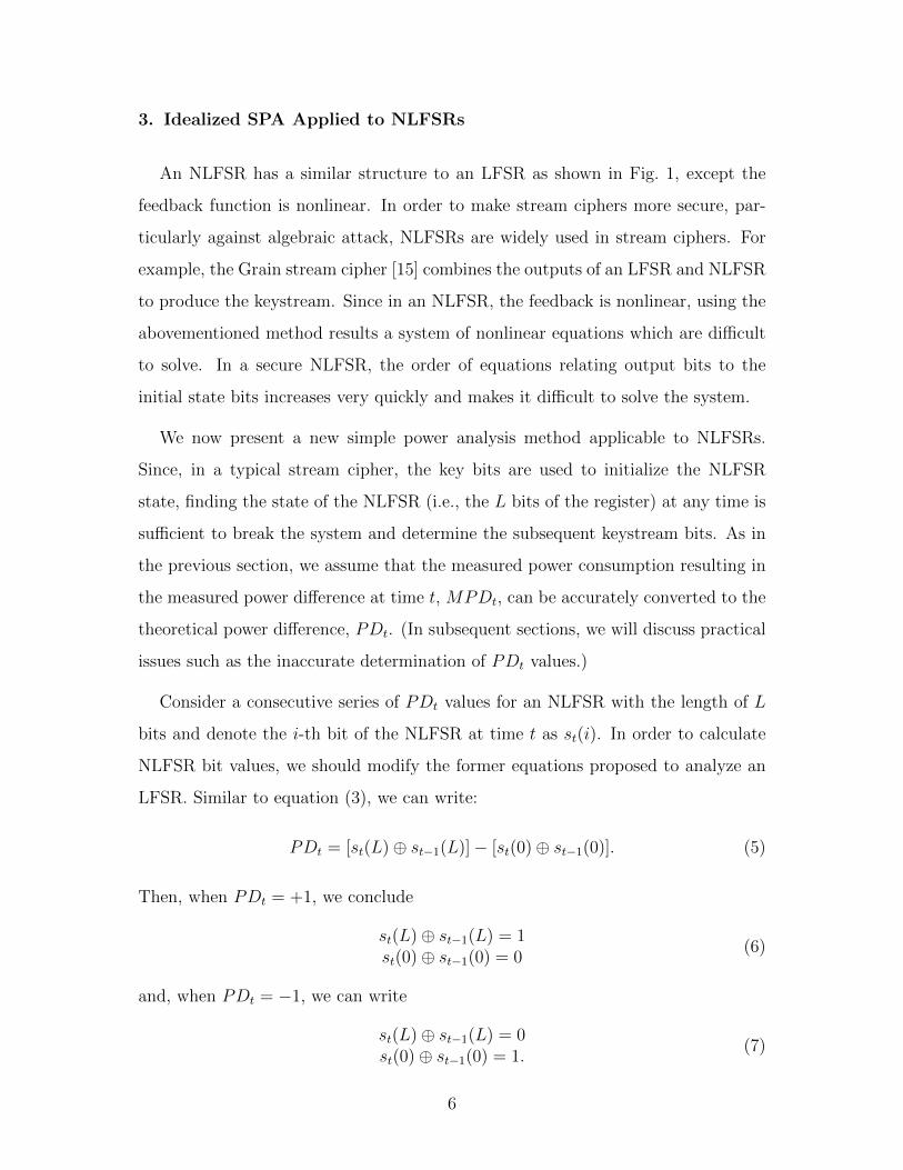
3. Idealized SPA Applied to NLFSRs

An NLFSR has a similar structure to an LFSR as shown in Fig. 1, except the

feedback function is nonlinear. In order to make stream ciphers more secure, par-

ticularly against algebraic attack, NLFSRs are widely used in stream ciphers. For

example, the Grain stream cipher [15] combines the outputs of an LFSR and NLFSR

to produce the keystream. Since in an NLFSR, the feedback is nonlinear, using the

abovementioned method results a system of nonlinear equations which are difficult

to solve. In a secure NLFSR, the order of equations relating output bits to the

initial state bits increases very quickly and makes it difficult to solve the system.

We now present a new simple power analysis method applicable to NLFSRs.

Since, in a typical stream cipher, the key bits are used to initialize the NLFSR

state, finding the state of the NLFSR (i.e., the L bits of the register) at any time is

sufficient to break the system and determine the subsequent keystream bits. As in

the previous section, we assume that the measured power consumption resulting in

the measured power difference at time t, MPDt, can be accurately converted to the

theoretical power difference, PDt. (In subsequent sections, we will discuss practical

issues such as the inaccurate determination of PDt values.)

Consider a consecutive series of PDt values for an NLFSR with the length of L

bits and denote the i-th bit of the NLFSR at time t as st(i). In order to calculate

NLFSR bit values, we should modify the former equations proposed to analyze an

LFSR. Similar to equation (3), we can write:

PDt = [st(L)⊕ st−1(L)]− [st(0)⊕ st−1(0)]. (5)

Then, when PDt = +1, we conclude

st(L)⊕ st−1(L) = 1st(0)⊕ st−1(0) = 0

(6)

and, when PDt = −1, we can write

st(L)⊕ st−1(L) = 0st(0)⊕ st−1(0) = 1.

(7)

6

When PDt = 0, the two bracketed XOR results of equation (5) are both equal to

either 0 or 1 and we can write

st(L)⊕ st−1(L) = st(0)⊕ st−1(0). (8)

As long as PDt 6= 0, we can find a relation between two consecutive values of the

NLFSR bits, using equation (6) or (7).

To analyze the NLFSR, we must obtain L consecutive bits of the NLFSR. Equa-

tions (6) and (7) could determine the relation between two bits of the NLFSR when

PDt = +1 or PDt = −1. However, when PDt = 0, we cannot use equations (6)

and (7) directly. Replacing t with t + L in (4), results in

|PDt+L| = st+L(L)⊕ st+L−1(L)⊕ st+L(0)⊕ st+L−1(0). (9)

Now, XORing both sides of (4) and (9) leads to

|PDt| ⊕ |PDt+L| = st(L)⊕ st−1(L)⊕ st(0)⊕ st−1(0)⊕ st+L(L)

⊕st+L−1(L)⊕ st+L(0)⊕ st+L−1(0) (10)

= st(0)⊕ st−1(0)⊕ st(2L)⊕ st−1(2L)

where we have made use of st+j(i) = st(i + j). Also, it can be shown that

PDt + PDt+L = [st(2L)⊕ st−1(2L)]− [st(0)⊕ st−1(0)]. (11)

The value of PDt+i must be +1, 0 or −1 implying |PDt+i| ∈ {0, 1}. Since

|PDt| ⊕ |PDt+L| will be either 1 or 0, if PDt = 0, then we can write equation (6)

or (7) for PDt+L if |PDt+L| is 1 and using equation (10) find the relation between

st(0) and st−1(0). For example, let us assume PDt = 0. If PDt+L = +1 or −1,

then st(2L) ⊕ st−1(2L) and st(L) ⊕ st−1(L) are known from either equation (6) or

(7) (with t replaced with t + L) and since the left side of equation (10) is known

from power measurements then st(0)⊕ st−1(0) can be inferred. If PDt+L = 0, then

power differences from cycle t + 2L must be considered.

Now using equations (6) or (7) and (10), if necessary, the relationships between

L pairs of consecutive bits are known. Although the actual values of the bits are

7

not known, there are only two possibilities and both can be tested to determine

which results in the correct state of the NLFSR. Since for this method, the feedback

relation is not used, we can use the approach for both an NLFSR and LFSR. This

method has the advantage that there is no need to solve a system of equations.

From equation (5), it is easy to see that the probability of PDt equal to zero

is 12. Hence, we need to obtain PDt+L for, on average, 1

2of L consecutive PDt

values. On average, 12

of the values of PDt+L are equal to zero and we need to

collect PDt+2L values. In other words, on average for 12

of L consecutive bits we

are targeting, we need to collect PDt+L values; for 14

of the L consecutive bits,

we need to collect PDt+2L values, etc. In practical applications to analyze the

sequence of an NLFSR, it is sufficient to find any consecutive L bits of the NLFSR.

Hence, the analysis initially collects a number of consecutive power samples and then

analyzes the values. In order to estimate the probability of a successful analysis,

we assume n × L consecutive power difference values have been collected. The

probability of all PDt+iL values being zero for 0 ≤ i < n and a fixed value of t (and

therefore not being usable to determine bits in the register) is 2−n. If we assume the

occurrence of PDt = 0 for different values of t are independent, then, given n × L

power difference values, the probability that this is enough samples to analyze the

NLFSR is [1− 2−n]L. For L� 2n, this probability is approximately 1− 2−nL. So,

for example, for L = 80, 800 consecutive power samples (i.e., n = 10) will allow

successful analysis with a probability of about 92%.

4. Power Consumption of D Flip-flops

The analysis outlined in the previous section and the previous work such as

[12] is idealized in that it assumes a perfect determination of PDt values from

measured power differences, MPDt. In this and the following sections, we consider

the practical issues associated with applying simple power analysis to a simulated

CMOS circuit realization of an NLFSR when the measured power difference may

not lead to the correct determination of PDt. For the principal focus of our analysis,

8

Figure 2: Classical architecture of D flip-flop.

we shall consider cryptographic circuits constructed using a classical positive edge

triggered D flip-flop, as shown in Fig. 2. In Section 8, we also briefly examine

simulated results for another typical D flip-flop construction for CMOS circuits.

The classical D flip-flop includes six NAND gates (T1, T2, ..., T6), two independent

inputs (clock and D) and two dependent outputs (Q and Q). The D flip-flop state, Q,

changes only at the rising edge of the clock. The dynamic power (which is typically

the dominant factor in power consumption of CMOS circuits) of the D flip-flop

depends on the number of changing gates (resulting in transistor state changes).

4.1. Power Consumption at the Rising Edge of the Clock

Previously proposed attacks assume the power consumption of the circuit at the

rising (i.e., triggering) edge of the clock. Since, at the rising edge of the clock, the

value of the register can change, we can conclude some gates and transistor states

are changed. As can be seen from Fig. 2, when D = 0 and Q = 0, at the rising edge

of the clock only T3 changes, and, when D = 1 and Q = 1, at the rising edge only

T2 changes. When D = 0 and Q = 1, at the rising edge of the clock, three gates

(T3, T5 and T6) change. Three gates (T2, T5 and T6) also change, when D = 1

and Q = 0. Hence, we expect more power to be consumed at the rising edge when

D = 1 and Q = 0 or when D = 0 and Q = 1, compared to when D = 0 and Q = 0

or when D = 1 and Q = 1. In other words, when there is a D flip-flop state change,

we expect more power consumption. This is consistent with the Hamming distance

9

Figure 3: Power consumption of single D flip-flop at the rising edge (in watts) versus time (inseconds), when (a) D = 0 and Q = 0, (b) D = 0 and Q = 1, (c) D = 1 and Q = 0, (d) D = 1 andQ = 1.

power model used in our proposed analysis and the approach of others.

In Fig. 3, the power consumption of a single D flip-flop for different inputs and

outputs is illustrated. In Fig. 3, the vertical axis represents the consumed power

and the horizontal axis represents time. The rising clock edge occurs at t = 0 with

the transition time of the rising clock edges set to 20 ns. In this paper, we have used

Cadence Virtuoso Spectre Circuit Simulator version 5.10.41 to obtain the power

consumption of the circuit. All the circuits here are prototyped in TSMC 180 nm

standard cell CMOS technology. The supply voltage of all circuits is 1.8 volts and

the experiments have been done assuming room temperature and default noise.

For an LFSR or NLFSR, the power consumption of the circuit at the rising edge

of the clock corresponds to the summation of power consumption of each single D

flip-flop (plus a small amount of power consumption due to the combinational logic

in the feedback and output functions). Hence, HDt, in general, is expected to be

proportional to the summation of the consumed power of each D flip-flop. We refer

to SPA applied based on power consumption from the rising edge of the clock as

rising edge simple power analysis or RESPA.

10

Figure 4: Power Consumption of one D flip-flop at the falling edge (in watts) versus time (inseconds), when (a) D = 0 and Q = 0; (b) D = 0 and Q = 1; (c) D = 1 and Q = 0; (d) D = 1 andQ = 1.

4.2. Power Consumption at the Falling Edge of the Clock

Studying the architecture of the positive edge triggered D flip-flop, we can see

at the falling (i.e., non-triggering) edge of the clock, we have changes in some gates

and transistor states. When D = 1 and Q = 1, at the falling edge of the clock, one

gate will change (T2), and, when D = 0 and Q = 0, T3 will change. Meanwhile, for

D = 0 and Q = 1, two gates (T1 and T2), and, for D = 1 and Q = 0, three gates

(T1, T3 and T4) will change at the falling edge. The power consumption of a D

flip-flop at a falling edge of the clock for different D and Q are shown in Fig. 4 where

the vertical axis represents the consumed power and the horizontal axis represents

time. The falling clock edge occurs at t = 0, with the falling edge transition time of

20 ns.

Considering the consumed power at the falling edge of the clock to analyze the

cryptographic circuits has not been discussed in the previous literature. We refer to

this approach as falling edge SPA or FESPA. In the subsequent sections, we use the

power consumption of the circuit at the falling edge of the clock, in addition to the

rising edge, to analyze cryptographic circuits. Obviously, this technique is not only

applicable to stream ciphers and it could be applied to block ciphers and public key

cryptographic circuits, as well.

11

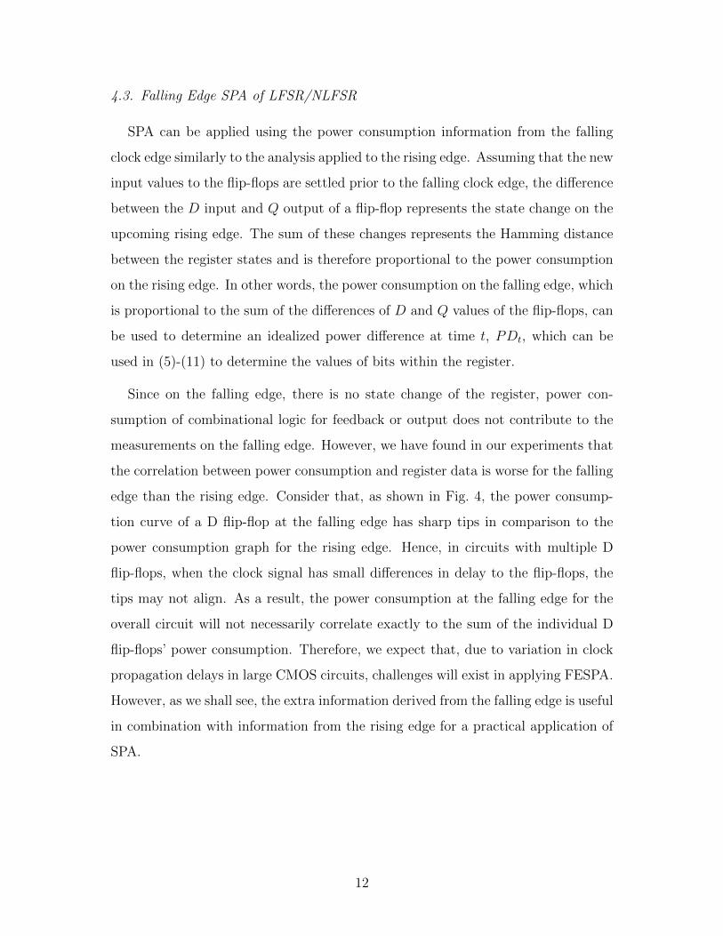
4.3. Falling Edge SPA of LFSR/NLFSR

SPA can be applied using the power consumption information from the falling

clock edge similarly to the analysis applied to the rising edge. Assuming that the new

input values to the flip-flops are settled prior to the falling clock edge, the difference

between the D input and Q output of a flip-flop represents the state change on the

upcoming rising edge. The sum of these changes represents the Hamming distance

between the register states and is therefore proportional to the power consumption

on the rising edge. In other words, the power consumption on the falling edge, which

is proportional to the sum of the differences of D and Q values of the flip-flops, can

be used to determine an idealized power difference at time t, PDt, which can be

used in (5)-(11) to determine the values of bits within the register.

Since on the falling edge, there is no state change of the register, power con-

sumption of combinational logic for feedback or output does not contribute to the

measurements on the falling edge. However, we have found in our experiments that

the correlation between power consumption and register data is worse for the falling

edge than the rising edge. Consider that, as shown in Fig. 4, the power consump-

tion curve of a D flip-flop at the falling edge has sharp tips in comparison to the

power consumption graph for the rising edge. Hence, in circuits with multiple D

flip-flops, when the clock signal has small differences in delay to the flip-flops, the

tips may not align. As a result, the power consumption at the falling edge for the

overall circuit will not necessarily correlate exactly to the sum of the individual D

flip-flops’ power consumption. Therefore, we expect that, due to variation in clock

propagation delays in large CMOS circuits, challenges will exist in applying FESPA.

However, as we shall see, the extra information derived from the falling edge is useful

in combination with information from the rising edge for a practical application of

SPA.

12

5. Categorization of Power Measurements

Previously proposed simple power analyses of stream ciphers have ignored the

effect of inaccurately mapping from analog MPD values to discrete theoretical PD

values caused by effects such as power consumption sources other than the flip-

flops (i.e., the combinational logic in the feedback or output functions) and clock

skew. In this section, we study the effect of inaccuracies in categorizing measured

power consumption for simple power analysis based on experimental results from

simulation.

When we measure the peak power consumption of the circuit at the clock edges

and subtract their values at consecutive rising/falling edges (to obtain MPD), we

have analog values, which we should map to discrete PD values, where PD ∈

{+1, 0,−1}. (For convenience, we often drop the subscript t when referring to

power difference values in this section.) In the following, we offer a method to

map or categorize MPD values to {+1, 0,−1}. Then we offer some techniques to

distinguish incorrectly categorized MPD, that is, incorrectly determined values for

PD. The categorized value for MPD (or the categorized PD) is denoted by PDc,

while the correct theoretical power difference based on actual data in the register is

simply notated PD. Hence, when we map the measured power difference at time t,

MPDt, to a categorized power difference PDct , a correct categorization would mean

that PDct = PDt.

It should be noted that if measured power differences are randomly mapped to

a category of {−1, 0,+1}, the probability that the categorization would be correct,

Pcorr, is given by

Pcorr =∑

i∈{−1,0,+1}

P{PDc = i|PD = i} · P{PD = i} (12)

where P{PD = i} represents the probability that a power difference equals i and

the conditional probability is calculated as P{PDc = i|PD = i} = P{PDc = i} =

P{PD = i} since the categorization is random relative to the actual PD value. Since

it is reasonable to assume in an LFSR or NLFSR that the probability of generating

13

0 and 1 are equal, the probability of PD = +1, PD = 0, and PD = −1 are .25,

.5 and .25, respectively. This results in the probability of correct categorization

being 37.5% and the probability of an incorrect categorization being 62.5%. These

numbers are useful as a frame of reference for the following discussion.

5.1. Categorizing MPD

In one simple approach to categorize the measured power difference (MPD) to

their corresponding PDc values, at first we sort MPD values in order of their value.

The smaller 25% of MPD values should be categorized to PDc = −1. The largest

25% of MPD values should be categorized to PDc = +1. The remaining MPD

values should be categorized to PDc = 0.

In our analysis, we use this method to categorize MPD. However, this method

is not perfect and some MPD values may be categorized incorrectly. We have

applied this method to an 80-bit NLFSR. The NLFSR used is equivalent to the

NLFSR used in the Grain stream cipher [15] and is defined in Appendix A. After

collecting 20000 power samples through simulation (using the structure of Fig. 2

with a 500 ps transition time) and applying our categorization method, we found

about 16 percent of rising edge MPD values were categorized incorrectly. Incorrect

categorization occurred for falling edge MPD values in about 32 percent of the cases.

More analysis on the experimental results shows the probabilities of incorrectly

categorizing an actual PD = +1 (or PD = −1) to PDc = −1 (or to PDc = +1)

is negligible. In other words, virtually all categorization errors occur by incorrectly

assigning +1 or −1 to 0, or 0 to +1 or −1.

Because of the abovementioned categorization errors we must modify the pro-

posed SPA in Section 3 for real applications. In doing so, we must ensure that we

can identify correctly categorized power differences with high probability and must

reject power differences for which we are not confident in their correct categorization.

14

5.2. Basic Methods to Determine Correctly Categorized PD

Here we offer some techniques which help us to find, with high probability, correct

PDc, i.e., correctly categorized MPD values such that the measurement determined

power difference, PDc, equals the power difference that should result from the actual

data, PD. For each of the proposed methods, we have determined experimentally

(through simulation of the 80-bit NLFSR) the probability of correct categorization,

as well as the probability that the condition has occurred to allow us to categorize

an MPD value with confidence.

5.2.1. Rising Edge/Falling Edge Equivalence

When we measure the power consumption of the circuit in simple power analysis,

we can assume we have access to power consumption at both rising and falling

edges. Based on experiments for our system, the probability of an incorrect PDc in

RESPA and FESPA are .160 and .320, respectively. Then, for any clock cycle, if the

categorized values are the same for both edges and we assume that the probability of

correctness for the rising edge and the falling edge are independent, the probability

that the categorized PD is incorrect is determined as the probability that both

values are wrong and is therefore given by .160 × .320 = .051. In other words, if

categorization using falling edge and rising edge show the same value, this value is

correct with a theoretical probability of .949, which is similar to the experimentally

measured probability of .950. This represents a much higher level of confidence then

taking, on their own, either the rising edge or falling edge categorization (which have

probabilities of .840 and .680, respectively). Our experiments show that we can use

this technique to ensure correct categorization for about 60% of the measurements

from different clock cycles, with this high probability.

5.2.2. Robust Threshold

Another technique to help categorize MPD values accurately is using a more

robust threshold value. In this technique, we change the threshold and, instead of

25%, we categorize the smallest and largest 12.5% as PDc = −1 and PDc = +1,

15

respectively, and the middle 25% as PDc = 0. In this approach, categorizations are

correct with higher probability. Obviously, this technique can be applied to 50% of

the MPD (for both rising edge and falling edge). Our experiments show that, using

this approach, categorization for the rising edge is correct with a probability of .955,

while for the falling edge categorization, the probability of correctness is .750.

5.2.3. Sequence Consistency

Another technique, which we call the sequence consistency method, can be used

to improve categorization success by distinguishing correct categorizations from in-

correct ones. To find the incorrect categorizations, we can use equation (11). In

(11), the right side of the equation cannot be larger than +1 or smaller than −1;

hence, at the left side PDt+L cannot be equal to PDt, unless both are equal to zero.

Extrapolating equation (11), if we add j consecutive PD terms separated by L clock

cycles, we getPDt + PDt+L + . . . + PDt+(j−1)L

= [st(jL)⊕ st−1(jL)]− [st(0)⊕ st−1(0)].(13)

The right side must be from the set {−1, 0,+1} and, hence, the summation of any

j consecutive PD values L bits apart can never be larger than one or smaller than

minus one. Hence, if PDt = +1, then PDt+L and PDt−L must be either 0 or −1.

Similarly, PDt = −1 implies PDt+L = 0 or +1 and PDt−L = 0 or +1. If in any

sequence of PDct+iL values, we see two consecutive +1 values, we know that at least

one of them is categorized incorrectly. In other words, a correct sequence of PDc

values separated by L clock cycles, starting with a value of PDc = +1, must be

followed by a string of some number of values of PDc = 0 and then PDc = −1. In

contrast, a +1 value, any number of 0 values and then +1 indicates an incorrect

categorization, i.e., at least one PDc value is wrong. Similar analysis is true for a

sequence starting with PDc = −1.

In applying the sequence consistency technique, consider a sequence of three

categorized values: {PDct−L, PDc

t , PDct+L}. We can increase our confidence in a

correct categorization of PDct by considering the full sequence. For example, in

RESPA, if we have categorized each value of sequence {PDct−L, PDc

t , PDct+L} as

16

{+1,−1,+1} independently, the probability that PDct is correct is .840 (as deter-

mined by experiment). However, using the sequence consistency method, the proba-

bility of correctness of PDct for this sequence is increased to .984. If the categorized

sequence is {+1,−1,+1}, it means the actual PD sequence could be {0,−1, 0},

{0,−1,+1}, {+1,−1, 0}, {+1,−1,+1}, {0, 0, 0}, {0, 0,+1} or {+1, 0, 0}. Sequences

like {−1, 0, 0} are not possible as the actual sequence because we assume the prob-

ability of categorizing an actual PD = −1 as PDc = +1 is negligible. If any of

the first four sequences is the actual sequence, our categorization of PDct = −1

is correct and if any of the last three cases is the actual sequence, our categoriza-

tion is incorrect. The probability of occurrence for each sequence is equal to 116

,

except {0, 0, 0} which is 18. If we let the probability of any individual PDt being

correctly categorized be represented by Pcr, then the probability of an individual

PDt = 0 incorrectly categorized as +1 is equal to 12(1 − Pcr). (A similar proba-

bility occurs for incorrectly categorizing 0 to −1). Hence, the probability of actual

sequence {0,−1,+1} categorized as {+1,−1,+1} is equal to 12(1− Pcr)PcrPcr. The

probability of observing a sequence as {+1,−1,+1} is equal to summation of the

probabilities of occurrence of each sequence (either 116

or 18) times the probability of

categorizing that sequence as {+1,−1,+1}. From all possible sequences, we have

selected 8 sequences with high probability for our purpose and list them in Table 1.

Using the occurrence of these sequences on either the rising or falling edge as indica-

tors of correct categorizations could increase the probability of categorizing MPD

values correctly to a probability of .913 (as determined by experiment) and could

be applied to 78% of all measured power differences.

6. Advanced Categorization Methods

In our analysis, we require PDc with high probability of correctness. In the

previous section, we have introduced some methods to distinguish PDc which are

likely to be correct. In this section, we derive PDc with even higher probability of

correctness by selecting PDc values for which at least two of the above techniques

are applicable. We list them as follows:

17

Sequence Probability of PDct = PDt Probability of PDc

t = PDt

{PDct−L, PDc

t , PDct+L} for rising edge for falling edge

{+1,−1,+1} .984 .918{−1,+1,−1} .984 .918{+1, 0,−1} .968 .852{−1, 0,+1} .968 .852{0,+1,−1} .906 .781{0,−1,+1} .906 .781{−1,+1, 0} .906 .781{+1,−1, 0} .906 .781

Table 1: Probability of PDct = PDt for sequences of three PDc values for rising edge (Pcr = .840)

and falling edge (Pcr = .680).

(I) RE/FE Equivalence and Robust Threshold on RE

In this case, two categorized PDc values of rising edge and falling edge that

are the same and consistent with the robust threshold of the rising edge are

assumed correct. The experimental results from the 80-bit NLFSR show that

the probability of correctness for this case is .992, while the probability that

such consistency occurs for a given clock cycle is .315.

(II) RE/FE Equivalence and Robust Threshold on FE

A similar approach could be taken based on consistency with the categorization

based on the falling edge robust threshold. The experimental results show

the probability of correctness for this case is .974, while the probability of

occurrence of this case is .326.

(III) RE/FE Equivalence and Sequence Consistency

In this case, the two categorized values of rising edge and falling edge are the

same and the sequence consistency method confirms their correctness. Our

experiments show the correctness of PDc values in this case are .987, while

the probability of such an occurrence is .326.

(IV) Robust Threshold on RE/FE and Sequence Consistency

In this case, the PDc value is determined by the robust threshold of RESPA

18

Scenario PDct−2L PDc

t−L PDct PDc

t+L PDct+2L Probability

A X X ±1 X X .233

B X ±1 C X X .124C X ±1 0 X X .054

D ±1 0 C X X .029E ±1 0 0 X X .013

F C C 0 ±1 X .016

G 0 C 0 ±1 X .007

H C 0 0 ±1 X .007I 0 0 0 ±1 X .003

J C C 0 0 ±1 .004

K C 0 0 0 ±1 .002

L 0 C 0 0 ±1 .002M 0 0 0 0 ±1 .001

N ±1 C 0 0 ±1 .002

Table 2: Cases used to determine st(0)⊕ st−1(0).

or FESPA and the sequence method confirms it. Experiments show the prob-

abilities of correctness and occurrence are .998 and .219, respectively.

During the determination for any PDc, if at least one of cases I, II, III or IV

occurs, we assume that the categorization is correct. Based on the experimental

results, the probability of at least one of the mentioned cases occurring for a PDc

is .467 and the probability of correctness is .975.

7. Analyzing the NLFSR

We now consider the application of simple power analysis to the 80-bit NLFSR,

using the probabilities derived from experimental results for the categorization

methodologies previously described. On average, upon categorization of power mea-

surement values, we expect that at least one of cases I, II, III, and IV occurs for

.467 × 80 ≈ 37 PDc values of the 80 bits and the resulting PDc values are correct

with high probability of about .975. However, half of these PDc values will be equal

to 0 and, as indicated in the Section 3, we cannot use them to obtain information

on the NLFSR state bits.

19

Based on equations (6), (7) and (8), if we know PDt−L = +1 or −1, we can

find st(0)⊕ st−1(0). Similarly, there are many scenarios for which knowing PDt−2L,

PDt+L, or PDt+2L are equal to +1 or −1 will allow us to determine st(0)⊕ st−1(0).

In Table 2, we have listed possible scenarios for PDct−2L, PDc

t−L, PDct , PDc

t+L and

PDct+2L that we could use to guess the relationships between st(0) and st−1(0). In

the table, if from cases I, II, III or IV, PDc = ±1, we present it as ±1 and, if from

cases I, II, III or IV, PDc = 0, we present it as 0. If cases I, II, III and IV are

not applicable to PDc, we cannot be confident in the categorization of PDc and we

present it as C. If the value of PDc is not critical to defining the scenario in the

table, we show it with “X” (i.e., the value is a “don’t care”).

The probability of occurrence for each scenario in the table is given in the right

column. To calculate the listed probabilities, we assume the probability of PDct =

+1 or −1 is equal to the probability of PDct = 0 and is therefore given by .467

2= .233.

The probability of PDct = C is 1 − .467 = .533. Hence, the probability of scenario

A is equal to the probability of PDct = +1 or −1 and is therefore .233. The

probability of scenario B is the probability of PDct−L = +1 or −1 and PDc

t = C,

which is .233 × .533 = .124, where we have made the reasonable assumption that

the power differences at times separated by L clock cycles are independent. For

scenario C, the probability is calculated as .233× .233 = .054, which is equal to the

probability of PDct−L = +1 or −1 and PDc

t = 0. The rest of the probabilities of

Table 2 are calculated similarly.

All cases in the table are mutually exclusive; hence, the sum of the right column,

which equals about .49, is the probability that one of the scenarios occurs. Therefore,

we have about 80 × .49 ≈ 39 relationships of pairs of consecutive bits with high

probability of correctness and we can guess the remaining 80−39 = 41 relationships.

Considering the scenarios of Table 2, on average we would need about 55 PDc values

with high probability in order to determine the 39 XOR relationships with high

probability. This is explained as follows. If either scenario A or B occurs, (which

will happen with a probability of .233+.124=.357), we need only one PDc with high

20

probability. If scenarios C, D or F occur (which will happen with the probability of

.099), we need two PDc values with high probability of correctness. For scenarios

E, G, H and J, we need to know three PDc values and for I, K, L and N, we have to

know four PDc values. For M, we need to know five PDc values. Hence, on average,

we need to know 80× (1× .357 + 2× .099 + 3× .031 + 4× .009 + 5× .001) ≈ 55 PDc

values with high probability of correctness to know 39 bits of the NLFSR. The 55

PDc values are drawn from power consumption data spanning from t−2L to t+2L

for values of t spanning L = 80 bits of the register. Hence, power trace information

is required over a span of 5L = 400 clock cycles.

As studied before, if any of cases I, II, III or IV could be applied to determine

a PDc value, it is correct with the probability of .975. Hence, assuming 55 PDc

values are used to generate the 39 XOR expressions and the correctness of each PDc

is independent, the set of 39 XOR expressions are correct with the probability of

.97555 = .248. In other words, if we apply our analysis using a typical set of power

consumption values, our analysis will be successful about 25% of the time.

If we have enough power samples and we could apply our analysis to 16 in-

dependent sets of measured power consumption values, with the probability of

1−(1− .248)16 = .990, we have at least one successful analysis. The resulting overall

complexity of the analysis can be derived by considering the exhaustive search for

the 41 XOR expressions not found from the PDc values for each of the 16 appli-

cations of the analysis giving a computational complexity of about 16 × 241 ≈ 245

operations, where an operation involves the analysis of the PDc values for the cases

of Table 2. In comparison, a cryptanalysis based on exhaustively searching for the

proper state of the NLFSR would be expected to take about 280 steps. Hence, signif-

icant reduction in the analysis complexity can be achieved by examining the power

consumption information and applying simple power analysis.

To decrease the complexity of the analysis, we can expand the cases of I, II, III

and IV to include the basic categorization techniques of Section 5.2. For example,

we may assume that, if PDc from the falling edge and rising edge are the same, this

21

PDc is correct with high probability (Section 5.2.1). Also, if the robust threshold

on the rising edge (not falling edge) is applicable, the PDc may be assumed to be

correct with high probability (Section 5.2.2). Now if one of cases I, II, III, or IV or

the categorizations based on Sections 5.2.1 or 5.2.2 can be used, the probability of

correctness of PDc values is decreased to .964. However, one of these cases occurs

with a probability of .784. Hence, the presented probabilities in Table 2 change. For

example, the probabilities for scenarios A, B, and C change to .392, .085, and .154,

respectively. The summation of the probabilities for all scenarios is now about 80%.

Using the new probabilities, we can obtain about .80× 80 ≈ 64 XOR relationships

based on about 107 PDc values (spanning 5L = 400 clock cycles) which are all

correct with an expected probability of about .964107 ≈ .02. This gives an expected

success rate for the analysis of only 2%. However, we can increase the probability of

success to more than 98%, if we repeat the analysis on 200 independent sets of power

trace data. The resulting complexity would be about 200× 216 ≈ 224 operations.

Although, the first approach has higher complexity (245 operations), it requires

fewer number of power samples (i.e., 16 × (5 × 80) = 6400 clock cycles of power

samples for the 80-bit NLFSR). However, the second approach, with lower compu-

tational complexity (224 operations) needs more power samples (i.e., 200×(5×80) =

80000 samples).

8. Further Practical Issues

In this section, we discuss further practical issues, including the brief considera-

tion of a typical D flip-flop construction for CMOS circuits.

8.1. Power Consumption of Another D Flip-flop Construction

In Fig. 5, another D flip-flop construction targeted to CMOS is illustrated [16].

This structure is often a preferred structure in CMOS circuits because of its low

power consumption and fewer number of transistors. Using our simulation tools, we

have obtained and plotted simulation results for power consumption for both rising

22

Figure 5: Another typical architecture of D flip-flop.

(triggering) and falling (non-triggering) edges of this alternate D flip-flop structure.

These are presented in Fig. 6 and Fig. 7, using a 20 ns transition time.

It can be seen that, as can be expected by examining the circuit operation, again

there is dynamic power consumption on both the rising and falling clock edges.

However, notably, the power consumption for cases where the flip-flop state does

not change is visibly insignificant. Hence, for a single flip-flop, the cases of a change

in state (with significant power consumption) and the cases of no change in state

(with negligible power consumption) are easily distinguishable by examining power

measurements. The resulting implication is that the Hamming distance between

clock cycles for the full LFSR or NLFSR is expected to be correlated to the measured

power at the clock edge. Consequently, we have applied our simulations to the full

NLFSR based on the flip-flop of Fig. 5 using a clock with a 50 ps transition time.

Utilizing the power difference categorization techniques of Section 5.1 resulted in

measured power differences being correctly categorized 62% of the time for the rising

edge and 50% of the time for the falling edge. Such probabilities are clearly better

than the 37.5% probability of correctly categorizing if the power differences were

randomly categorized and may therefore form the basis of a power analysis attack.

However, compared to probabilities of 84% and 68% (for rising and falling edges,

respectively) for the D flip-flop of Fig. 2, the correct categorization probability

is substantially worse and the attack will not have as much success as the results

discussed in Section 7. We conjecture that these poorer results occur because, as

can be seen in Fig. 6, the spikes of power consumption are narrow and occur at

different points in time for the 0 to 1 and 1 to 0 changes. As a result, for this flip-

flop, the overall power consumption on a rising clock edge does not correlate well

23

Figure 6: Power Consumption of one D flip-flop at the rising edge (in watts) versus time (inseconds), when (a) D = 0 and Q = 0; (b) D = 0 and Q = 1; (c) D = 1 and Q = 0; (d) D = 1 andQ = 1.

to the Hamming distance in the NLFSR data compared to the classical D flip-flop

of Fig. 2. In this paper, we have used the power consumption data generated from

simulation of an NLFSR based constructed using the D flip-flop structure of Fig. 2

to illustrate the potential applicability of the attack.

8.2. Limitations of Simulated Power Values

In this section, we identify some of the further challenges that will occur in a

practical realization of an attack on a CMOS circuit. For example, the instanta-

neous power consumption of a CMOS circuit will also be influenced by many factors

other than the dynamic power consumption of the basic NLFSR circuit. Capaci-

tances from circuit wiring, I/O pads, and decoupling capacitors will all contribute

to modifying the timing of current drawn from the power supply. Added capaci-

tive effects are likely to make distinguishing between rising and falling edge power

consumption more challenging, particularly in high speed circuits.

Further, the CMOS circuit is likely to have other functionality executing at the

same time as the NLFSR circuit. This will add further dynamic power consumption

to the overall circuit and will obscure the power directly consumed by the NLFSR.

The attacker must understand the context of the circuit under analysis and find

mechanisms to isolate the power consumed by only the NLFSR circuit. Finally,

24

Figure 7: Power Consumption of one D flip-flop at the falling edge (in watts) versus time (inseconds), when (a) D = 0 and Q = 0; (b) D = 0 and Q = 1; (c) D = 1 and Q = 0; (d) D = 1 andQ = 1.

implementing an attack that relies on the instantaneous power associated with rising

and falling clock edges requires precise timing of the power measurements. This may

certainly be a challenge in a high speed circuit with a low clock period. As well, clock

skew within the circuit may result in spreading out the contribution of power from

individual flip-flops and making categorizations from the measured power differences

to the theoretical power differences more inaccurate.

Although there are further practical issues to be considered when implementing

an attack on real (rather than simulated) hardware, the results of this work clearly

indicate that a simple power analysis attack has the potential to be applicable to

practical scenarios where the idealized assumption relating measured power differ-

ences to the cipher data with perfect accuracy does not apply.

9. Conclusion

In this paper, we have proposed a simple power analysis of NLFSR, a component

typically found in stream ciphers. Also, we consider power consumption of a typical

CMOS D flip-flop and propose use of power samples at the falling (or non-triggering)

edge of the clock for the analysis. Furthermore, we applied the analysis to an 80-bit

NLFSR using simulated power trace data for a 180 nm CMOS circuit. We have

25

shown that if we use falling edge and rising edge power consumption information

and the proposed techniques in this paper, we can successfully analyze with high

probability the NLFSR with computational complexity of about 245 operations us-

ing about 6400 power samples or 224 using about 80000 power samples. This is

significantly less than the complexity of 280 for exhaustive search for the NLFSR

state. These techniques apply equally to LFSRs.

These results indicate that practical implementation of stream ciphers based on

either LFSRs and/or NLFSRs may be vulnerable to side channel attacks and that it

is not a prerequisite of the attack that the assumption of idealized perfect mapping

from power difference measurements to cipher data holds true. Hence, care must be

taken to design implementations which do not leak power consumption information.

In future work, we intend to apply the analysis directly to the application of practical

CMOS implementations of stream ciphers with multiple LFSRs/NLFSRs, such as

the Grain stream cipher. One other possible avenue for future work would be to

analyze the applicability of the SPA approach to a circuit making use of transistor

models for the CMOS gates, instead of simulation results from CAD tools.

Appendix A. NLFSR Feedback Function

The feedback used for the 80-bit NLFSR in this paper is identical to the feedback

used in the NLFSR of the stream cipher Grain v0 [15] and is given by:

st(80) = st(63)⊕ st(60)⊕ st(52)⊕ s(45)⊕ st(37)⊕ st(33)⊕ st(28)

⊕st(21)⊕ st(15)⊕ st(9)⊕ st ⊕ st(63)st(60)⊕ st(37)st(33)

⊕st(15)st(9)⊕ st(60)st(52)st(45)⊕ st(33)st(28)st(21)

⊕st(63)st(45)st(28)st(9)⊕ st(60)st(52)st(37)st(33)

⊕st(63)st(60)st(21)st(15)⊕ st(63)st(60)st(52)st(45)st(37)

⊕st(33)st(28)st(21)st(15)st(9)⊕ st(52)st(45)st(37)st(33)st(28)st(21).

26

References

[1] A. Barbero, G. Horler, A. Kholosha, and O. Ytrehus, ‘Lightweight Cryptogra-

phy for RFID Devices’, IET Conference on Wireless, Mobile and Multimedia

Networks, pp. 294–297, 2008.

[2] N. Fournel, M. Minier, and S. Ubeda, ‘Survey and Benchmark of Stream Ci-

phers for Wireless Sensor Networks’, Workshop in Information Security Theory

and Practices (WISTP 2007), Lecture Notes in Computer Science, vol. 4462,

Springer, pp. 202–214, 2007.

[3] P.C. Kocher, ‘Timing Attacks on Implementations of Diffie-Hellman, RSA,

DSS, and Other Systems’, Proceeding of the 16th Annual International Cryp-

tology Conference (CRYPTO ’96), Lecture Notes in Computer Science, vol.

1109, Springer, pp. 104–113, 1996.

[4] P.C. Kocher, J. Jaffe, and B. Jun, ‘Differential Power Analysis’, Proceedings of

the 19th Annual International Cryptology Conference on Advances in Cryptol-

ogy (CRYPTO ’99), Lecture Notes in Computer Science, vol. 1666, Springer,

pp. 388–397, 1999.

[5] J.-J. Quisquater and D. Samyde, ‘ElectroMagnetic Analysis (EMA): Measures

and Counter-Measures for Smart Cards’, International Conference on Research

in Smart Cards (E-smart 2001), Lecture Notes in Computer Science, vol. 2140,

Springer, pp. 200–210, 2001.

[6] K. Gandolfi, C. Mourtel, and F. Olivier, ‘Electromagnetic Attacks: Con-

crete Results’, Workshop on Cryptographic Hardware and Embedded Systems

(CHES 2001), Lecture Notes in Computer Science, vol. 2162, Springer, pp.

251–261, 2001.

[7] S. Chari, J.R. Rao, and P. Rohatgi, ‘Template Attacks’, Workshop on Cryp-

tographic Hardware and Embedded Systems (CHES 2002), Lecture Notes in

Computer Science, vol. 2523, Springer, pp. 13–28, 2003.

27

[8] J.J. Hoch and A. Shamir, ‘Fault Analysis of Stream Ciphers’, Workshop on

Cryptographic Hardware and Embedded Systems (CHES 2004), Lecture Notes

in Computer Science, vol. 3156, Springer, pp. 240–253, 2004.

[9] W. Fischer, B.M. Gammel, O. Kniffler, and J. Velten, ‘Differential Power Anal-

ysis of Stream Ciphers’, Proceedings of the 7th Cryptographers’ track at the

RSA Conference (CT-RSA 2007), Lecture Notes in Computer Science, vol.

4377, Springer, pp. 257–270, 2007.

[10] J. Lano, N. Mentens, B Preneel, and I. Verbauwhede, ‘Power Analysis of Syn-

chronous Stream Ciphers with Resynchronization Mechanism’, presented at

Workshop on the State of the Art of Stream Ciphers (SASC 2004), Brugge,

Belgium, Oct. pp.327-333, 2004.

[11] R. Ebrahimi Atani, S. Mirzakuchaki, S. Ebrahimi Atani, and W. Meier, ‘On

DPA-Resistive Implementation of FSR-based Stream Ciphers using SABL Logic

Styles’, International Journal of Computers, Communications and Control, vol.

3, No. 4, pp. 324–335, 2008.

[12] S. Burman, D. Mukhopadhyay, and K. Veezhinathan, ‘LFSR Based Stream

Ciphers Are Vulnerable to Power Attacks’, INDOCRYPT 2007, Lecture Notes

in Computer Science, vol. 4859, Springer, pp. 384–392, 2007.

[13] A.A. Zadeh and H.M. Heys, ‘Applicability of Simple Power Analysis to Stream

Ciphers Using Multiple LFSRs’, Proceedings of Canadian Conference on Elec-

trical and Computer Engineering (CCECE 2012), Montreal, May 2012.

[14] A.J. Menezes, P.C. van Oorschot, and S.A. Vanstone, Handbook of Applied

Cryptography, CRC Press, 1997.

[15] M. Hell, T. Johansson, and W. Meier, ‘Grain - A Stream Cipher for Constrained

Environments’, ECRYPT Stream Cipher Project Report 2005/001, 2005, avail-

able from www.ecrypt.eu.org/stream.

28

[16] N.H.E. Weste and D.M. Harris, CMOS VLSI Design: A Circuits and Systems

Perspective, 4th edition, Addison-Wesley, 2011.

29