Embed Size (px)
Citation preview

Basis, The Journal of Basic Science 1 (2013) 1-12
1
SIMPLE EQUATION OF STATE
FOR WATER, CARBON DIOXIDE, METHANE, AND THEIR MIXTURES
Sergey Pivovarov
Institute of Experimental Mineralogy RAS, 142432 Chernogolovka, Moscow district, Russia
E-mail: [email protected]
Published online 05.03.2013
ABSTRACT
The PVT data of H2O (0-800oC, up to 60 kbar), CO2 (0÷800
oC, up to 30 kbar) and
CH4 (-110÷350oC, up to 10 kbar) were approximated by equation
P, bar = RTm{1 + Am – Bm/(1 + βm) – Cm2{1 – (1 –(Am)
2)exp( –(Am)
2)} + Dm
3}
Here R is gas constant (0.0831441 dm3barmol
-1K
-1), T is absolute temperature, m is
molarity of gas (moles per dm3), A, B, β, C, D are model parameters (below q = 298.15/T):
AH2O = 0.022699 + 0.0049722q/(1+0.539q12
)
BH2O = 1.0629qexp{2.768(q-1)}
βH2O = 0.060225q1.9
+ 0.20051q3.5
+ 0.0035436q14
CH2O = 0.017461q2.9
/(1+6.701q2.3
) + 0.0016763q2.4
/(1+1.993q8.3
)
DH2O = 0.000057006q + 0.000022393q/(1+1.54q9)
ACO2 = 0.053736/(1 + 0.2497q)
BCO2 = 0.16508qexp{0.673(q-1)}
βCO2 = 0.016222q
3.4
CCO2 = 0.030447q
3.1/(1+6.015q
2.7) + 0.0071431q
2.3
DCO2 = 0.00061996q
ACH4 = 0.049878/(1+0.03094q)
BCH4 = 0.088477qexp{0.2873(q-1)}
βCH4 = 0.0041616q
3
CCH4 = 0.008267q
2.9/(1+2.267q
2.2) + 0.0025764q
2
DCH4 = 0.00040808q
The properties of H2O-CO2-CH4 mixtures (0-700oC, up to 6 kbar) are consistent with
Ax = ∑AiXi
Bx = Bxo – 2kCO2H2O(BCO2
BH2O)0.5
XCO2XH2O – 2kCH4H2O(BCH4
BH2O)0.5
XCH4XH2O
Bxo = (∑Bi
1/2Xi)
2; kCO2H2O = 0.2286 - 0.6123q
5 + 0.6888q
7 – 0.256q
9
kCH4H2O = 0.3595 -1.653q5 + 2.037q
7 -0.731q
9; (kCH4CO2
= 0)
βx = ∑βiXi
Cx = {∑Ci1/3
Xi}3
Dx = {∑Di1/4
Xi}4
The fugacity of gas in the H2O-CO2-CH4 mixture may be found from f i= RTmiYi and
lnYi = (Ai + Ax)m –{2Bi0.5
(Box0.5
–∑jkijBj0.5
Xj) –Bx(βi/βx)}ln(1 +βxm)/βx – Bx(βi/βx)m/(1 +βxm)
– 1.5(CiCx2)1/3
m2[1 – exp{–(Axm)
2}] – Cxm
4AiAxexp{– (Axm)
2} + (4/3)(DiDx
3)1/4
m3

● Green zone, theoretical: reviews and new approaches; ready for use
2
INTRODUCTION
The equation of state is a very useful tool for understanding of various geological phenomena. Since the geology deals with complex mixtures of fluids at high parameters, high accuracy of calculations seems to be inaccessible. Because of this, multiparametric and, potentially exact approaches are weakly applicable, since they are not efficient and even senseless (e.g., negative volume) above the experimental range. Thus, less accurate, but simpler approaches, having ability for more or less successful extrapolation, and which may be easily extended to complex gas mixtures, are more relevant. The aim of present study is a creation of equation of state, which is 1) simple and convenient 2) more or less accurate 3) applicable to complex mixtures 4) applicable from low up to extreme T-P conditions. This study is focused on most important system H2O-CO2. However, both these fluid components are rather peculiar substances, and the model was also tested on PVT data for methane. METHODS
The PVT data for methane were taken from equation of state of Setzmann and Wagner (1991; 90-620 K, up to 10 kbar), and finally were used up to 2 kbar in the range 160-400 K and up to 0.5 kbar at 500-600 K. Above 2 kbar, the model was fitted to experimental data from Robertson and Babb (1969; 35÷200
oC, to 10 kbar) and Morris (1984; -20÷150
oC, to
6.9 kbar). Data from Kortbeek and Schouten (1990; 25oC, to 10 kbar) were not used because
of small inconsistence with data from Robertson and Babb (1969), which were preferred due to large temperature range covered by experiment. Data from Tsiklis (1971a; 50-400
oC, to 8.5
kbar) were not used because of systematic deviation from other studies by 0.6 percent. The PVT data for water at 0-800
oC up to 1 kbar were taken from Rivkin and
Aleksandrov (1984) steam tables. Above 1 kbar, model was fitted to the volumetric data from Bridgman (1912; 0÷80
oC, to 12 kbar), Grindley and Lind (1971; 25÷150
oC, to 8 kbar),
Hilbert et al. (1981; 20÷600oC, to 4 kbar), and values deduced from sound velocity
measurements: Wiryana et al. (1998; 80÷200oC, 2.5-35 kbar), Abramson and Brown (2004;
100÷400oC, 10÷60 kbar). The data from Burnham et al. (1969; 20÷900
oC, to 8.9 kbar) were
not used because of systematic deviation from other studies (at 8 kbar and 20÷400oC, the
density is underestimated by 0.6 %), except excellent agreement with data from Bridgman 1935 (0÷100
oC, to 12 kbar), which also were rejected. The data from Bridgman (1942; 25-
175oC, up to melting curve, 36.56 kbar in maximum) were not used because these data were
measured as increments in volume between 5 kbar and higher pressure (thus, “true” value for density at 5 kbar should be selected arbitrarily). The data from Von Köster and Frank (1969; 25÷600
oC, to 10 kbar) are in excellent agreement with results of other studies up to 150
oC,
but at higher temperatures and highest pressures they seems to be in error (at 8 kbar and 600
oC, disagreement with data from Burnham et al., 1969, is 1.9 %; at 10 kbar and 400
oC,
disagreement with data from Abramson and Brown, 2004, is 1.2 %). The same is probably true for the data from Von Maier and Frank (1966; 200÷850
oC, up to 6 kbar; at 6 kbar and
800oC, disagreement with data from Burnham et al., 1969, is 3 %). Data from fluid inclusion
studies: Brodholt and Wood (1994; 900÷1600oC, 9.5-25 kbar), Withers et al. (2000;
710÷1100oC, 14÷40 kbar), Frost and Wood (1997; 1000÷1400
oC, 14.5 kbar) also were not
considered because of small inconsistence with data from Abramson and Brown (2004) which were preferred. The values tabulated by Rice and Walsh (1957) were not used because it is prognostic equation of state.
In case of carbon dioxide, the model was fitted to volumetric data from Michels and Michels (1935; 0-150
oC, to 0.25 kbar) Michels et al., (1935; 0÷150
oC, up to 3.1 kbar),
Vukalovich et al. (1962, 1963; 40÷750oC, up to 0.6 kbar), Kennedy (1954; 0-1000
oC, up to
1.4 kbar), Jůza et al. (1965; 50-475oC, up to 4 kbar), Tsiklis et al. (1971b; 50-400
oC up to 7
kbar), Shmonov and Shmulovich (1974; 408.2-707.5oC, up to 8 kbar), and data deduced from
sound velocity measurements: Giordano et at. (2006; 27-427oC, up to 80 kbar). There is large
(up to 4.4 %) discrepancy among various data, and construction of self-consistent calibration dataset is a problem, which has no unique solution. The following data were rejected from

Basis, The Journal of Basic Science 1 (2013) 1-12
3
final calibration dataset: from Kennedy (1954) above 800oC, from Tsiklis et al. (1971b) above
5 kbar, from Shmonov and Shmulovich (1974) above 5 kbar and all data at 707.5oC, from
Giordano et al. (2006) above 200oC.
The selected data were used for construction of isotherms at round temperatures. Above 1 kbar, data were used with large increments (1 or 2 kbar to 10 kbar, 5 kbar to 20 kbar and then 10 kbar). If necessary, experimental data were interpolated (or, slightly extrapolated) to round temperatures and pressures with use of approximations: V = V(tr
oC) + a(t-tr) + b(t-tr)
2 (1)
ρ = ρ(Pr, bar) + c(P-Pr)/(1+d(P-Pr)) (2) Here tr and Pr are round temperature and pressure, a, b, c, and d are adjusting parameters.
The isotherms were converted into “second virial function”, (Z-1)/ρ, where ρ is density in g/cm
3, and Z = PV/RT is compressibility factor. Further the best fit values of
parameters were determined at each round temperature, and initial approximation was found for each parameter. Then the completely parameterized equation was optimized with use of all selected data. In case of carbon dioxide and methane, the data on saturation pressure were not used, and thus, the model was applied solely for the range above ~ 0.9Tcr. In case of water, temperature dependence of parameters was optimized for the range 200-800
oC,
whereas in the range 0-150oC the best fit parameters at each round temperature were found
with use of values of fugacity at saturation (this gives independent relation between parameters). Then the equation (for range 200-800
oC) and best fit values (in the range 0-
150oC) for the most stable parameter were approximated with general equation. This equation
was fixed, and procedure was repeated until the general approximation for the last parameter was found. RESULTS AND DISCUSSION
The following equation was found more or less applicable: P, bar = RTm{1 + Am – Bm/(1+ βm) – Cm
2{1 – (1 –(Am)
2)exp( –(Am)
2)} + Dm
3} (3)
Here R is gas constant (0.0831441 dm3barmol
-1K
-1), T is absolute temperature, m is
molarity of gas (moles per dm3; MH2O = 18.0152 g/mol, MCO2
= 44.0098 g/mol, MCH4 = 16.043
g/mol), A, B, β, C, D – are model parameters (below q = 298.15/T): AH2O = 0.022699 + 0.0049722q/(1+0.539q
12) (4)
BH2O = 1.0629qexp{2.768(q-1)} (5)
βH2O = 0.060225q1.9
+ 0.20051q3.5
+ 0.0035436q14
(6)
CH2O = 0.017461q2.9
/(1+6.701q2.3
) + 0.0016763q2.4
/(1+1.993q8.3
) (7)
DH2O = 0.000057006q + 0.000022393q/(1+1.54q9) (8)
ACO2
= 0.053736/(1 + 0.2497q) (9)
BCO2 = 0.16508qexp{0.673(q-1)} (10)
βCO2 = 0.016222q
3.4 (11)
CCO2 = 0.030447q
3.1/(1+6.015q
2.7) + 0.0071431q
2.3 (12)
DCO2 = 0.00061996q (13)
ACH4
= 0.049878/(1+0.03094q) (14)
BCH4 = 0.088477qexp{0.2873(q-1)} (15)
βCH4 = 0.0041616q
3 (16)
CCH4 = 0.008267q
2.9/(1+2.267q
2.2) + 0.0025764q
2 (17)
DCH4 = 0.00040808q (18)
● Green zone, theoretical: reviews and new approaches; ready for use
4
Parameter A was used twice: as an offset of second virial coefficient (second virial
coefficient at infinite temperature) and as an exponential factor, which is similar to that in
Benedict-Webb-Rubin equation (Benedict et al., 1940). This is artificial, and probably,
0.0 0.2 0.4 0.6 0.8
Density, g/cm
0
100
200
300
400
P,
bar
H O2
3
270 Co300 C
o330 Co360
Co380 Co400 Co
420 Co
450
Co
800 Co(a)
0.6 0.8 1.0 1.2
Density, g/cm
2
4
6
8
P, k
ba
r
400
Co
700
Co
200
Co
100 Co
25 Co
3
H O2
300
Co
500
Co
600
Co
800
Co
900
Co
(b)
0.0 0.2 0.4 0.6 0.8 1.0
Density, g/cm
0
50
100
150
P,
bar
CO2
3
280 K3
00 K
320 K
340
K
400 K
800 K(c)
0.7 0.9 1.1 1.3 1.5
Density, g/cm
2
4
6
8
P, k
ba
r
400
Co
700
Co
200
Co
100
Co
25 Co
3
CO2
50 Co
(d)
0.0 0.1 0.2 0.3 0.4
Density, g/cm
0
20
40
60
80
100
P,
bar
CH4
3
160 K1
80 K200 K22
0 K
250
K
500 K(e)
0.3 0.4 0.5 0.6
Density, g/cm
2
4
6
8
10
P, k
ba
r
400
Co30
0 Co
200
Co
100
Co
25 Co
- 20
Co
3
CH4
(f)
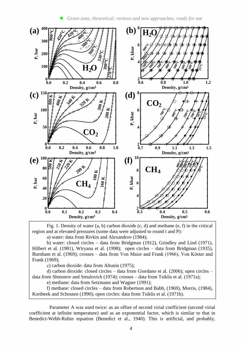
Fig. 1. Density of water (a, b) carbon dioxide (c, d) and methane (e, f) in the critical
region and at elevated pressures (some data were adjusted to round t and P):
a) water: data from Rivkin and Alexandrov (1984);
b) water: closed circles – data from Bridgman (1912), Grindley and Lind (1971),
Hilbert et al. (1981), Wiryana et al. (1998); open circles – data from Bridgman (1935),
Burnham et al. (1969); crosses – data from Von Maier and Frank (1966), Von Köster and
Frank (1969);
с) carbon dioxide: data from Altunin (1975);
d) carbon dioxide: closed circles – data from Giordano et al. (2006); open circles –
data from Shmonov and Smulovich (1974); crosses – data from Tsiklis et al. (1971a);
e) methane: data from Setzmann and Wagner (1991);
f) methane: closed circles – data from Robertson and Babb, (1969), Morris, (1984),
Kortbeek and Schouten (1990); open circles: data from Tsiklis et al. (1971b).

Basis, The Journal of Basic Science 1 (2013) 1-12
5
senseless correlation, but this simplification was found more or less applicable. The pre-
exponential factor (1-(Am)2) may be omitted, and recalibration of the model gives
approximately similar quality of description. However, this factor simplifies calculation of
fugacity.
Fig. 1 shows behavior of Eq. (3) in the critical region and at elevated pressures. The
modeled critical temperatures are 394.5, 31.6, and -81.4oC for water, carbon dioxide and
methane (experimental values are 374.1, 31.1, and -82.6oC), i.e. the model of water is most
inaccurate. The accuracy of the model with respect to selected data is generally better than 0.3
% in molar volume, except critical region (deviations in pressure up to 10 % for water, and up
to 3 % for carbon dioxide and methane).
0.8 1.0 1.2 1.4 1.6Density, g/cm
10
20
30
40
50
60
P, k
ba
r
3
H O2
100
Co20
0 Co
300
Co
400
Co
700
Co
1100
Co
1600
Co
(a)
1.3 1.5 1.7 1.9 2.1Density, g/cm
10
20
30
40
50
60
70
P, k
ba
r
3
400
Co
300
Co
200 Co
100 Co
50 Co
CO2
(b)
0 1 2 3Density, g/cm
0
300
600
900
P, k
ba
r
3
219 K
293 K110 K
3700 K
4330 K
3280 K3830 K
4090 K
4480 K
5270 K
CH
CO2
4
H O2
(c)
(5500 K)
(3800 K)
1 2 3 4Density, g/cm
0
5000
10000
15000
P, k
ba
r
H O2T ~ 10000 - 50000 K
3
(d)
Fig. 2. Density of water, carbon dioxide and methane at high pressures (some data
were adjusted to round t and P):
a) water: closed circles – data from Wiryana et al. (1998), Abramson and Brown
(2004); open circles – data from Brodholt and Wood (1993), Frost and Wood (1997),
Withers et al. (2000);
b) carbon dioxide: data from Giordano et al. (2006);
c) density of shock-compressed methane (circles: Radousky et al., 1990), water
(diamonds: Lysenga et al., 1982), and carbon dioxide (boxes: Nellis et al., 1991).
Experimental or, in brackets, theoretical temperatures are indicated near each point. Solid
curves were calculated with use of approximations: T = To + a(ρ-ρo)b, where a and b are
adjusting parameters.
d) density of shock-compressed water in the dense plasma region; data from
Celliers et al. (2004, open circles) and from Podurets et al. (1972, solid circle); solid curve
is the same as in Fig. 2c.

● Green zone, theoretical: reviews and new approaches; ready for use
6
In Fig. 2, the model calculations are compared with experimental data at high
pressures. Within the present approach, the values of density of water from fluid inclusion
studies (Fig. 2a, open circles) are slightly inconsistent with values obtained from sound
velocity measurements (Fig. 2a, closed circles). In the range 700-1100oC, the model deviates
from results of fluid inclusion studies by 1-2 %, which is experimental uncertainty of these
measurements.
As may be seen in Fig. 2b, the model deviates by 2.7 % in maximum from values
deduced from sound velocity by Giordano et al. (2006). The 400oC data seem to be
inconsistent with lower temperature data (the best fit parameters, optimized for each isotherm
and plotted against temperature, exhibit large step between 300 and 400oC). It should be
noted, that the values above 50 kbar were not really measured: for the measurements of sound
velocity in the diamond anvil, it is necessary to know the values of refractive index; these
values were measured up to 48 kbar and extrapolated to higher pressures. Thus, the values of
sound velocity as well as density above 48 kbar should be considered as extrapolated ones.
Up to 50 kbar, the present model is consistent with these data within the experimental error, 2
%, as estimated by Giordano et al. (2006).
Within 2-4 % the model agrees with Hugoniot data up to 800 kbar (Fig. 2c) and
gives, at least, not senseless results for the dense plasma region (>2000 kbar; Fig. 2d).
The common mixing rules may be guessed on basis of common sense. For instance,
the equation of state of water at very high pressure is simply
P ~ RT×DH2Om4 (19)
One may imagine that the compressed water consists of monomeric and dimeric molecules:
P ~ RT×DH2O(m1 + 2m2)4 = RT(D1
1/4m1 + D2
1/4m2)
4 (20)
Here m1 and m2 are molarities of monomeric and dimeric molecules, D1 = DH2O and D2 =
16DH2O are model parameters for monomeric and dimeric water. So on, the mixture of
components “1” and “2” may be modeled with use of the following mixing rule:
Dx = (D11/4
X1 + D21/4
X2)4 (21)
Similar considerations give general mixing rule, which is referred below as “n+1 rule”:
Nx = (ΣNi1/(n+1)
Xi)n+1
(22)
Here N is model parameter, and n is power factor of molarity in the equation of state, Z =
PV/RT = f(m). As it was found by Benedict et al. (1942), similar relation is consistent with
behavior of mixtures of hydrocarbons.
Another semi-empirical rule may be deduced from Van der Waals equation:
P = RT/(V-b) – a/V2 = RT(m + bm
2 + cm
3 + dm
4…..) – am
2 (23)
Here c = b2, d = b
3, etc. As it was suggested by Van der Waals (1881), parameter b of mixture
(“uncompressible volume”) is additive function of composition:
bx = ΣXibi (24)
Based on this relation, one may obtain the common mixing rule for parameters b, c = b2, d =
b3, etc (see Eq. 23):
Basis, The Journal of Basic Science 1 (2013) 1-12
7
Nx = (ΣNi1/n
Xi)n (25)
As above, N is model parameter, and n is power factor of molarity in the equation of state Z =
PV/RT = f(m). This relation is referred below as “n rule”.
As it was suggested by Van der Waals (1881), parameter “a” in the Eq (23) is
consistent with “n + 1 rule” (Eq . 22). For binary mixture of “inert components”, it is:
ax = (Σai0.5
Xi)2 = X1
2a1 + X2
2a2 + 2(a1a2)
0.5X1X2 (26)
If the specific interaction of component is significant, the additional parameter is necessary:
ax = X12a1 + X2
2a2 + 2(1-k12)(a1a2)
0.5X1X2 = (Σai
0.5Xi)
2 – 2k12(a1a2)
0.5X1X2 (27)
Here k12 is so called “coupling parameter”. The value k12 > 0 indicates repulsive interaction,
whereas k12 < 0 corresponds to attractive interaction. If to suggest, that the parameter “a” is
formation constant of dimeric molecules, the value 2(1-k12)(a1a2)0.5
is formation constant of
dimer, composed of two components.
0 200 400 600P, bar
0.3
0.5
0.7
0.9
1.1
1.3
Z =
PV
/RT
CH - COt = 50 C
CH0.8CH + 0.2CO0.5CH + 0.5CO0.2CH + 0.8COCO
4
4
4
4
2
2
2
2
o4 2
(a)
0 200 400 600P, bar
0.9
1.0
1.1
1.2
Z =
PV
/RT
CH - COt = 300 C
CH0.8CH + 0.2CO0.5CH + 0.5CO0.2CH + 0.8COCO
4
4
4
4
2
2
2
2
o4 2
(b)
0 200 400 600 800 1000P, bar
0.0
0.2
0.4
0.6
0.8
1.0
1.2
1.4
Z =
PV
/RT
CO
0.8CO + 0.2H O
2
22
0.6CO + 0.4H O2
2
0.4CO + 0.6H O2
2
0.2CO + 0.8H O2
2
H O2
H O - COt = 300 Co
2 2(c)
0 200 400 600 800 1000P, bar
0.2
0.4
0.6
0.8
1.0
1.2
1.4
Z =
PV
/RT
CO
0.8CO + 0.2H O
2
22
0.6CO + 0.4H O2
2
0.4CO + 0.6H O2
2
0.2CO + 0.8H O2
2
H O2
H O - COt = 400 Co
2 2(d)
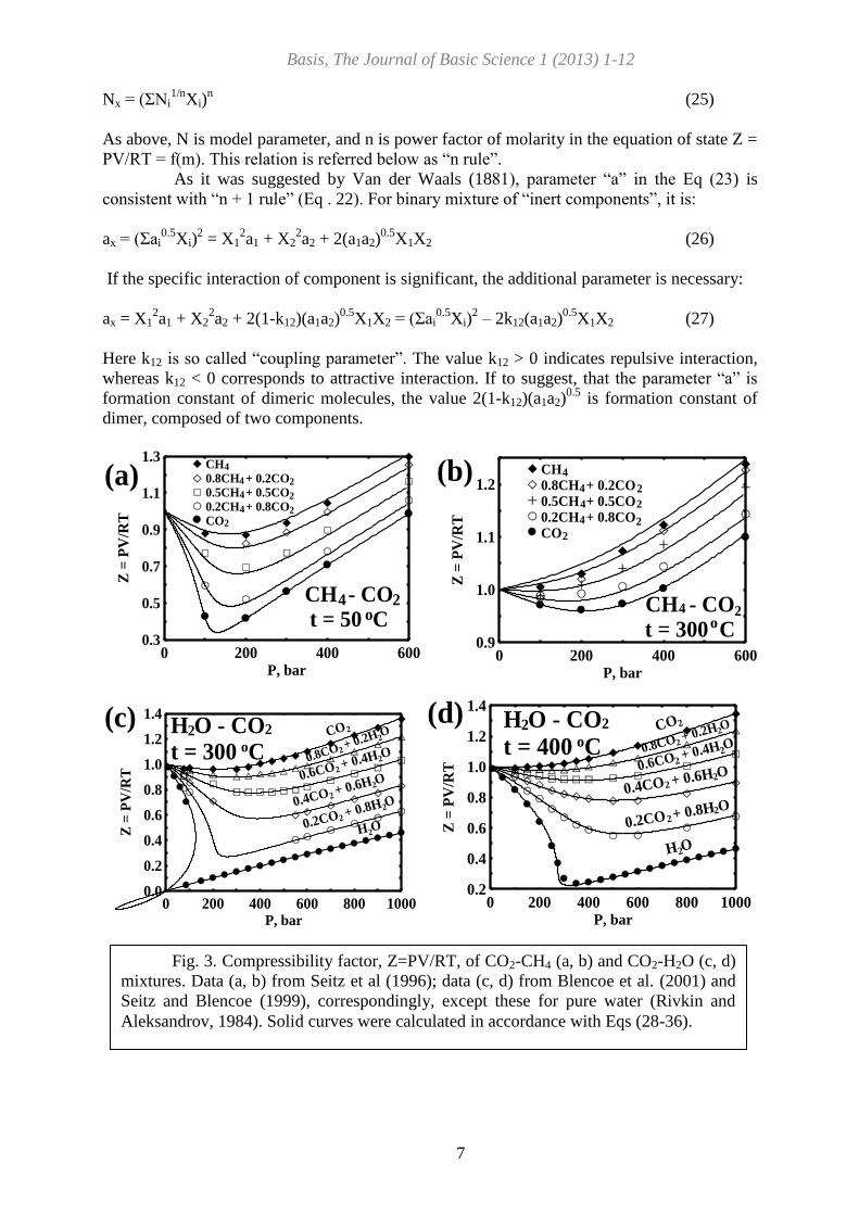
Fig. 3. Compressibility factor, Z=PV/RT, of CO2-CH4 (a, b) and CO2-H2O (c, d)
mixtures. Data (a, b) from Seitz et al (1996); data (c, d) from Blencoe et al. (2001) and
Seitz and Blencoe (1999), correspondingly, except these for pure water (Rivkin and
Aleksandrov, 1984). Solid curves were calculated in accordance with Eqs (28-36).

● Green zone, theoretical: reviews and new approaches; ready for use
8
By tries and errors, the following relations were found to be applicable for H2O-
CO2-CH4 mixtures (see Figs 3 and 4):
Ax = ∑AiXi (28)
Bx = Bo
x - 2kCO2H2O{BCO2BH2O}
1/2XCO2
XH2O - 2kCH4H2O{BCH4BH2O}
1/2XCH4
XH2O (29)
Box = {∑Bi
1/2Xi}
2 (30)
βx = ∑βiXi (31)
Cx = {∑Ci1/3
Xi}3 (32)
Dx = {∑Di1/4
Xi}4 (33)
kCO2H2O = 0.2286 - 0.6123q5 + 0.6888q
7 – 0.256q
9 (34)
kCH4H2O = 0.3595 -1.653q5 + 2.037q
7 -0.731q
9 (35)
(kCO2CH4 = 0) (36)
Here, as above, q is 298.15/T. The mixing rule for parameters Ax and βx was found close to “n
rule” (Eq. 25), whereas parameters Bx, Cx and Dx are consistent (or almost consistent) with
“n+1 rule” (Eq. 22). In case of aqueous mixtures, there is small repulsive (“hydrophobic”)
interaction, which is distinctive at low pressures, but fast decreases with density. Such
behavior may be simulated solely via adjustment of term Bm/(1+βm).
0.0 0.2 0.4 0.6 0.8 1.0X
20
28
36
44
52
V,
cm
/m
ol
3
CO2
H O - COt = 400 C
2 2o
2 kbar
3 kbar
4 kbar
5 kbar
(a)
0.0 0.2 0.4 0.6 0.8 1.0X
20
28
36
44
52
V,
cm
/m
ol
3
2 kbar
3 kbar
4 kbar
5 kbar
6 kbar
H O - COt = 600 C
2 2o
CO2
(b)
0.0 0.2 0.4 0.6 0.8 1.0X
20
40
60
80
100
120
140
V,
cm
/mol
3
0.5 kbar
CH4
0.8 kbar
1 kbar
2 kbar
H O - CHt = 400 Co
2 4(c)
0 100 200 300 400t C
2.5
3.0
3.5
4.0
4.5
5.0
log
KH
CH4
CO2
k = 0
CH4 H2O
k = 0CO2 H2O
o
(d)
Fig. 4 Molar volume of CO2-H2O (a,b) and CH4-H2O (c) mixtures and Henry
constant (d) of carbon dioxide and methane in water: data (a, b) from Sterner and
Bodnar (1991, open circles) and from Shmulovich et al. (1980, solid circles); data (c)
from Shmonov et al. (1993, open circles) and from Sretenskaya et al. (1986, solid
circles); data (d) from Fernández-Prini et al. (2003); solid curves were calculated in
accordance with Eqs (28-36); dashed curves (d) were calculated with kij = 0.

Basis, The Journal of Basic Science 1 (2013) 1-12
9
To obtain the approximations for the coupling parameters (Eqs 34 and 35), the
values of Henry constant (see Fig. 4d) were simply converted into coupling parameters, and
these values were approximated (all volumetric data for mixtures were ignored). The values
of Henry constant for carbon dioxide above 200oC and for methane above 300
oC were found
inconsistent with the model and were rejected (perhaps, this is due to uncertainty of the model
in the critical region). In general, specific interaction is small: the prediction based on
properties of pure components overestimates solubility of gases at 100-370oC by 2-3 times
(dashed curves in Fig 4d; below 100oC, the model of water is overparameterized and thus,
behavior of coupling parameter in this range has no deep sense). It should be noted that this
deviation is likely a specific property of water (tendency to form clusters) rather than real
specific interaction. The model was tested also on data for helium (not shown here), and
absolutely identical deviation from solubility curve was obtained. In case of CH4-CO2
mixtures, the coupling parameter is slightly positive (~ 0-0.1). However, this effect is
comparable with experimental error, and coupling parameter was set to zero (see Fig 3ab).
The fugacity may be calculated with use of the following relations between the
compressibility factor Z=P/mRT and thermodynamic potentials:
dAex
/RT = {(Z-1)/m}dm (37)
dGex
/RT = (1/m)d(Z-1)m (38)
Gex
/RT = Aex
/RT + md(Aex
/RT)/dm = Aex
/RT + Z – 1 (39)
Z = 1 + Axm – Bxm/(1+ βxm) – Cxm2[1-{1-(Axm)
2}exp(-(Axm)
2)] + Dxm
3 (40)
Aex
/RT = Axm – Bxln(1+ βxm)/βx – 0.5Cxm2[1-exp(-(Axm)
2)] + (1/3)Dxm
3 (41)
Here Gex
and Aex
are Gibbs and Helmholtz excess energies, m is total molarity of the mixture.
For pure component, the fugacity f may be calculated from
f = RTmY (42)
Y = exp(Gex
/RT) (43)
Here Y is “absolute activity coefficient”. For the mixture, the absolute activity coefficient of
component, Yi is related with its mole fraction Xi:
lnYi = Gex
/RT + (1-Xi){d(Aex
/RT)/dXi}m, Xj/Xk = const (44)
The Eq. (44) is convenient for numerical differentiation. However, the Eq (41) is
relatively simple, and the absolute activity coefficient may be calculated analytically. The
result is:
lnYi = (Ai + Ax)m –{2Bi0.5
(Box0.5
–∑jkijBj0.5
Xj) –Bx(βi/βx)}ln(1 +βxm)/βx – Bx(βi/βx)m/(1 +βxm)
–1.5(CiCx2)1/3
m2[1 –exp{–(Axm)
2}] –Cxm
4AiAxexp{– (Axm)
2} + (4/3)(DiDx
3)1/4
m3 (45)
Here ∑j is sum for components other than “i”. With use of this relation, the Henry constant
(Fig. 4d) may be calculated from:
KH = f2/X2 (at f2 → 0) = RTm2Y2/{m2/m} = RTmY2 (46)
Here f2, x2, m2, Y2 – are fugacity, mole fraction, molarity, and absolute activity coefficient of
dissolved gas, m is total molarity (here, molarity of pure water at saturation).

● Green zone, theoretical: reviews and new approaches; ready for use
10
CONCLUDING REMARKS
In spite of strong non-ideality of fluid mixtures, the specific interaction of fluid
components is weak and may be accounted for via adjustment of terms related to second virial
coefficient. The contribution of specific interactions at high pressures is negligible.
Compressibility of substance at very high pressures is consistent with P ~ ρ4, and thus, the
repulsive branch of Lennard-Jones potential is close to ~ ρ3, or 1/r
9.
REFERENCES
Abramson E.H. and Brown J.M. (2004) Equation of state of water based on speeds
of sound measured in the diamond-anvil cell. Geochim. Cosmochim. Acta 68, 1827-1835.
Altunin V.V. (1975) Teplofizicheskie svoystva dvuokisi ugleroda (Thermophysical
properties of carbon dioxide, in Russ). Izdatelstvo Standartov, Moscow.
Benedict M., Webb G.B. and Rubin L.C. (1940) An empirical equation for
thermodynamic properties of light hydrocarbons and their mixtures. I. Methane, ethane,
propane, and n-butane. J. Chem. Phys. 8, 334-345.
Benedict M., Webb G.B. and Rubin L.C. (1942) An empirical equation for
thermodynamic properties of light hydrocarbons and their mixtures. II. Mixtures of methane,
ethane, propane, and n-butane. J. Chem. Phys. 10, 747-758.
Blencoe J.G., Cole D.R., Horita J. and Moline G.R. (2001) Experimental
geochemical studies relevant to carbon sequestration. In Proceedings of the First National
Conference on Carbon Sequestration, U.S. National Energy Technology Laboratory,
Washington.
Bridgman P.W. (1912) Thermodynamic properties of liquid water to 80oC and
12000 Kgm. Proc. Amer. Acad. Arts Sci. 48, 309-362.
Bridgman P.W. (1935) The pressure-Volume-Temperature relations of the liquid,
and the phase diagram of heavy water. J. Chem. Phys. 3, 597-605.
Bridgman P.W. (1942) Freezing parameters and compressions of twenty-one
substances to 50,000 kg/cm2. Proc. Amer. Acad. Arts Sci. 74, 399-424.
Brodholt J.P. and Wood B.J. (1994) Measurements of the PVT properties of water
to 25 kbars and 1600oC from synthetic fluid inclusions in corundum. Geochim. Cosmochim.
Acta 58, 2143-2148.
Burnham C.W., Holloway J.R., and Davis N.F. (1969) The specific volume of
water in the range 1000 to 8900 bars, 20o to 900
oC. Am. J. Sci. 267-A, 70-95.
Celliers P.M., Collins G.W., Hicks D.G., Koenig M., Henry E., Benuzzi-Mounaix
A., Batani D., Bradley D.K., Da Silva L.B., Wallace R.J., Moon S.J., Eggert J.H., Lee
K.K.M., Benedetti L.R., Jeanloz R., Masclet I., Dague N., Marchet B., Rabec Le Gloahec M.,
Reverdin Ch., Pasley J., Willi O., Neelly D., and Danson C. (2004) Electronic conduction in
shock-compressed water. Phys. Plasmas 11, L41-L44.
Fernández-Prini R., Alvares J.L., and Harvey A.H. (2003) Henry’s constant and
vapor-liquid distribution constants for gaseous solutes in H2O and D2O at high temperatures.
J. Phys. Chem. Ref. Data 32, 903-916.
Frost D.J., and Wood B.J. (1997) Experimental measurements of the properties of
H2O-CO2 mixtures at high pressures and temperatures. Geochim. Cosmochim. Acta 61, 3301-
3309.
Giordano V.M., Datchi F., and Dewaele A. (2006) Melting curve and fluid equation
of state of carbon dioxide at high pressure and high temperature. J. Chem. Phys. 125, 054504.
Grindley T. and Lind J.E. Jr. (1971) PVT properties of water and mercury. J. Chem.
Phys. 54, 3983-3989.
Hilbert R., Tödheide K., and Franck E.U. (1981) PVT data for water in the ranges
20 to 600oC and 100 to 4000 bar. Ber. Bunsenges. Phys. Chem. 85, 636-643.

Basis, The Journal of Basic Science 1 (2013) 1-12
11
Jůza J., Kmoníček V., and Šifner, O. (1965) Measurements of the specific volume
of carbon dioxide in the range of 700 to 4000b and 50 to 475oC. Physica 31, 1735-1744.
Kennedy G.C. (1954) Pressure-volume-temperature relations in CO2 at elevated
temperatures and pressures. Am. J. Sci. 252, 225-241.
Kortbeek P.J. and Schouten J.A. (1990) Measurements of the compressibility and
sound velocity in methane up to 1 GPa, revisited. Int. J. Thermophys. 11, 455-466.
Lysenga G.A., Ahrens T.J., Nellis W.J., and Mitchell A.C. (1982) The temperature
of shock-compressed water. J. Chem. Phys. 76, 6282-6286.
Michels A. and Michels C. (1935) Isotherms of CO2 between 0 and 150oC and
pressures from 16 to 250 atmospheres. Proc. Roy. Soc. A153, 201-214.
Michels A., Michels C., and Wouters N. (1935) Isotherms of CO2 between 70 and
3000 atmospheres (amagat densities between 200 and 600). Proc. Roy. Soc. A153, 214-224.
Morris E.C. (1984) Accurate measurements of the PVT properties of methane from
-20 to 150oC and to 690 MPa. Int. J. Thermophys. 5, 281-290.
Nellis W.J., Mitchell A.C., Ree F.H., Ross M., Holmes N.C., Trainor R.J., and
Erskine D.J. (1991) Equation of state of shock-compressed liquids: carbon dioxide and air. J.
Chem. Phys. 95, 5268-5272.
Podurets M.A., Simakov G.V., Trunin R.F., Popov L.V., and Moiseev B.N. (1972)
Compression of water by strong shock waves. Sov. Phys. JETP 35, 375-376.
Radousky H.B., Mitchell A.C., and Nellis W.J. (1990) Shock temperature
measurements of planetary ices: NH3, CH4, and “synthetic Uranus”. J. Chem. Phys. 93, 8235-
8239.
Rice M.H. and Walsh J.M. (1957) Equation of state of water to 250 kilobars. J.
Chem. Phys. 26, 824-830.
Rivkin S.L. and Aleksandrov A.A. (1984) Termodinamicheskie svoystva vodi i
vodyanogo para. (Thermodynamic properties of water and steam, in Russ). Energoatomizdat,
Moscow.
Robertson S.L. and Babb S.E.Jr. (1969) PVT properties of methane and propene to
10 kbar and 200oC. J. Chem. Phys. 51, 1357-1361.
Seitz J.C., Blencoe J.G., and Bodnar R.J. (1996) Volumetric properties for {(1-
x)CO2 + xCH4}, {1-x)CO2 + xN2}, and {(1-x)CH4 + xN2} at the pressures (9.94, 19.94, 29.94,
39.94, 59.93, 79.93, and 99.93) MPa and temperatures (323.15, 373.15, 473.15, and 573.15)
K. J. Chem. Thermodyn. 28, 521-538.
Seitz J.C. and Blencoe J.G. (1999) The CO2-H2O system. I. Experimental
determination of volumetric properties at 400oC. Geochim. Cosmochim. Acta 63, 1559-1569.
Setzmann U. and Wagner W. (1991) A new equation of state and tables of
thermodynamic properties for methane covering the range from the melting line to 625 K at
pressures up to 1000 MPa. J. Phys. Chem. Ref. Data 20, 1061-1155.
Shmonov V.M. and Shmulovich K.I. (1974) Molar volumes and equations of state
for CO2 between 100-1000oC and 2000-10000 bars. Dokl. Akad. Nauk SSSR 217, 205-209.
Shmonov V.M., Sadus R.J., and Franck E.U. (1993) High-pressure phase-equilibria
and supercritical PVT data of the binary water plus methane mixture to 723 K and 200 MPa.
J. Phys. Chem. 97, 9054-9059.
Shmulovich K.I., Shmonov V.M., Mazur V.A., and Kalinichev A.G. (1980) P-V-T
and activity concentration relations in the H2O-CO2 systhem (homogeneous solutions).
Geochem. Int. 17, 123-139.
Sretenskaya N.G., Zakirov I.V., Shmonov V.M., and Shmulovich K.I. (1986)
Vodosoderzhaschie fluidnie sistemi. In Experiment v reshenii aktual’nih zadach geologii
(Water-bearing fluid systems. In Experiment in solution of actual problems of geology, in
Russ). Nauka, Moscow.

● Green zone, theoretical: reviews and new approaches; ready for use
12
Sterner S.M., and Bodnar R.J. (1991) Synthetic fluid inclusions. X. Experimental
determination of the P-V-T-X properties in the CO2-H2O system to 6 kb and 700oC. Amer. J.
Sci. 291, 1-54.
Tsiklis D.S., Linshits L.R., and Tsimmerman S.S. (1971a) Molar volumes and
thermodynamic properties of methane at high pressures and temperatures. Dokl. Akad. Nauk
SSSR 198, 384-386.
Tsiklis D.S., Linshits L.R., and Tsimmerman S.S. (1971b) Measurement and
calculation of molar volumes of carbon dioxide at high pressure and temperature.
Teplofizicheskie Svoistva Veschestv i Materialov 3, 130-136
Van der Waals J.D. (1881) Die Kontinuität des gasförmigen und flüssigen
zustandes. Johann Ambrosium Barth Verlag, Leipzig.
Von Köster H. and Franck E.U. (1969) Das spezifische volumen des wassers bei
hohen drucken bis 600oC und 10 kbar. Ber. Bunsenges. Phys. Chem. 73, 716-722.
Von Maier S. and Franck E.U. (1966) Die Dichte des Wassers von 200 bis 850oC
und von 1000 bis 6000 bar. Ber. Bunsenges. Phys. Chem. 70, 639-645.
Vukalovich M.P., Altunin V.V., and Timoshenko N.I. (1962) Experimental study of
the specific volume of carbon dioxide at temperatures 200-750oC and pressures up to 600
kg/cm2. Teploenergetika 5, 56-62.
Vukalovich M.P., Altunin V.V., and Timoshenko N.I. (1963) Experimental
determination of the specific volume of carbon dioxide at temperatures 40-150oC and
pressures up to 600 kg/cm2. Teploenergetika 10, 85-88.
Wiryana S., Slutsky L.J., and Brown J.M. (1998) The equation of state of water to
200oC and 3.5 GPa: model potentials and the experimental pressure scale. Earth Planetary
Sci. Lett. 163, 123-130.
Withers A.C., Kohn S.C., Brooker R.A., and Wood B.J. (2000) A new method for
determining the P-V-T properties of high-density H2O using NMR: results at 1.4-4.0 GPa and
700-1100oC. Geochim. Cosmochim. Acta 64, 1051-1057.