Embed Size (px)
Citation preview
Simple Conceptual Models for
Tropical Ocean-Atmosphere Interactions
on Interannual Timescales
Diplomarbeit
Malte Jansen
Leibniz-Institut fur Meereswissenschaftenan der Universitat Kiel
Mathematisch-Naturwissenschaftliche Fakultatder Christian-Albrechts-Universitat zu Kiel
June 15, 2007
brought to you by COREView metadata, citation and similar papers at core.ac.uk
provided by OceanRep

Abstract
The parameters of simple conceptual models for the coupled atmosphere-ocean dy-namics in the tropics are fitted to observational data and it is analyzed how well thefitted models reproduce observed statistical properties from stochastic excitation,representing short-timescale ”weather noise”.
The El Nino Southern Oscillation (ENSO) is well described by the linear rechargeoscillator model. In the recharge oscillator picture, the oscillation is explained bythe recharging (discharging) of equatorial heat content during a La Nina (El Nino)event. On the other hand, the delayed action oscillator, in which the oscillation is dueto equatorial wave travel times, turns out to be the less reasonable approximation.The observed skewness and kurtosis of eastern Pacific (Nino3) sea surface temperature(SST) timeseries can be explained by nonlinear coupling of SST on thermocline depthanomalies and effects of seasonality.
The observed dynamics of the equatorial Atlantic also turns out to be described wellby the recharge oscillator model. An oscillatory mixed ocean dynamics-SST modeexists in boreal spring and summer, while the system is overdamped in fall and winter.No oscillatory coupled mode is found in the Indian Ocean. Instead, Indian OceanSST seems to be well described by a red noise process forced by ENSO.
Fitting a simple model for the interactions of the tropical Indian and Atlantic Oceanswith ENSO to observational data, it is found that the Indian Ocean tends to damp theENSO oscillation and is responsible for a frequency shift to shorter periods. However,forecast prediction skills can hardly be improved by explicitly including the IndianOcean SST, since the latter is strongly related to ENSO. The interactions betweenthe Atlantic Ocean and ENSO are generally weaker than between Indian Ocean andENSO. But some feedback from the Atlantic on ENSO seem to exist, which couldimprove forecast prediction skills.
Zusammenfassung
Die Parameter von einfachen konzeptionellen Modellen fur die gekoppelte Dynamikvon Ozean und Atmosphare in den Tropen werden an Beobachtungsdaten angepasst.Es wird analysiert wie gut die Modelle, angetrieben von stochastischer Anregung,die das kurzzeitskalige ”Wetter-Rauschen” darstellen soll, beobachtete statistischeEigenschaften des Systems reproduzieren.
Die El Nino Southern Oscillation (ENSO) wird gut durch das lineare ”recharge oscil-lator” Modell beschrieben. Im ”recharge oscillator” Bild wird die Oszillation durchdas Aufladen bzw. Entladen des aquatorialen Warmeinhaltes wahrend eines La Ninabzw. El Nino Ereignisses bedingt. Das ”delayed action oscillator” Modell hingegen,bei dem die Oszillation durch die Propagationszeit aquatorialer Wellen bedingt ist,erweist sich als weniger sinnvolle Approximation. Die beobachtete Schiefe und Kur-tosis der Ost-Pazifischen (Nino3) Meeresoberflachentemperatur (SST) Zeitreihe kanndurch nichtlineare Kopplung der SST an Anomalien in der Tiefe der Thermoklineund durch die Saisonabhangigkeit der Variabilitat erklart werden.
Auch die beobachtete Dynamik im Gebiet des aquatorialen Atlantiks lasst sich gutdurch das ”recharge oscillator” Modell beschreiben. Ein gedampft schwingendergekoppelter Ozean Dynamik-SST Mode existiert im borealen Fruhling und Sommer,wahrend das System in Herbst und Winter uberdampft ist. Im Indischen Ozean kannkein gekoppelter periodischer Mode gefunden werden. Stattdessen ist die SST desIndischen Ozeans gut beschrieben durch einen von ENSO angetriebenen ”red-noise”Prozess.
Mit Hilfe eines einfachen Modelles fur die Wechselwirkung des tropischen Indischenbeziehungsweise Atlantischen Ozeans mit ENSO wird gezeigt dass der Indische Ozeandampfend auf ENSO wirkt und fur eine erhohte ENSO-Frequenz verantwortlich ist.Dennoch kann die Qualitat von ENSO-Vorhersagen durch die explizite Berucksichti-gung des Indischen Ozeans kaum verbessert werden, da dieser selbst stark vom ENSOSignal dominiert ist. Die Wechselwirkungen zwischen dem Atlantik und ENSO sindallgemein schwacher als zwischen dem Indischen Ozean und ENSO. Jedoch scheintein gewisser Einfluss des Atlantiks auf ENSO zu existieren, der die Vorhersagbarkeitvon ENSO verbessern konnte.
Contents
Introduction 5
1 Data and Methods 7
1.1 Data . . . . . . . . . . . . . . . . . . . . . . . . . . . . . . . . . . . . 7
1.2 Fitting Methods . . . . . . . . . . . . . . . . . . . . . . . . . . . . . . 7
1.2.1 The Linear Regression . . . . . . . . . . . . . . . . . . . . . . 8
1.2.2 The Numerical Least-Squares Fit . . . . . . . . . . . . . . . . 10
1.2.3 A Monte Carlo Experiment to Review Fitting Methods . . . . 11
1.2.4 Seasonal Dependent Parameter Fits . . . . . . . . . . . . . . . 13
2 Simple Models for ENSO 14
2.1 Introduction . . . . . . . . . . . . . . . . . . . . . . . . . . . . . . . . 14
2.2 The Delayed Action Oscillator . . . . . . . . . . . . . . . . . . . . . . 16
2.2.1 Model Description . . . . . . . . . . . . . . . . . . . . . . . . 16
2.2.2 Parameter Fit to Nino3 Observational Data . . . . . . . . . . 18
2.2.3 The Delayed Oscillator Excited by Stochastic Forcing . . . . . 21
2.3 The Recharge Oscillator . . . . . . . . . . . . . . . . . . . . . . . . . 23
2.3.1 Model Description . . . . . . . . . . . . . . . . . . . . . . . . 23
2.3.2 Parameter Fit to Observational Data . . . . . . . . . . . . . . 25
2.3.3 The Recharge Oscillator Excited by Stochastic Forcing . . . . 28
2.4 The Simplest Recharge Oscillator . . . . . . . . . . . . . . . . . . . . 30
2.5 The Delayed Recharge Oscillator . . . . . . . . . . . . . . . . . . . . 32
3
4 CONTENTS
2.5.1 Model Description . . . . . . . . . . . . . . . . . . . . . . . . 32
2.5.2 Parameter Fit to Observational Data . . . . . . . . . . . . . . 33
2.5.3 The Delayed Recharge Oscillator Excited by Stochastic Forcing 35
2.6 A Nonlinear Extension of the Delayed Recharge Oscillator . . . . . . 37
2.7 Seasonality . . . . . . . . . . . . . . . . . . . . . . . . . . . . . . . . 40
2.7.1 The Recharge Oscillator Model with Seasonal Dependent Pa-rameters . . . . . . . . . . . . . . . . . . . . . . . . . . . . . . 40
2.7.2 A Seasonal Dependent Parameter Fit for the Simplest RechargeOscillator Model . . . . . . . . . . . . . . . . . . . . . . . . . 48
2.8 Summary and Discussion . . . . . . . . . . . . . . . . . . . . . . . . . 50
3 Atlantic and Indian Ocean 54
3.1 Introduction . . . . . . . . . . . . . . . . . . . . . . . . . . . . . . . . 54
3.2 An Atlantic Recharge Oscillator? . . . . . . . . . . . . . . . . . . . . 55
3.3 An Indian Ocean Recharge Oscillator? . . . . . . . . . . . . . . . . . 58
3.4 Summary and Discussion . . . . . . . . . . . . . . . . . . . . . . . . . 63
4 Tropical Oceans’ Interaction 66
4.1 Introduction . . . . . . . . . . . . . . . . . . . . . . . . . . . . . . . . 66
4.2 A Simple Model for the Tropical Oceans’ Interactions with ENSO . . 67
4.3 Indian Ocean-ENSO Interaction . . . . . . . . . . . . . . . . . . . . . 67
4.4 Atlantic Ocean-ENSO Interaction . . . . . . . . . . . . . . . . . . . . 72
4.5 A Coupled Model for the Interaction of All Tropical Oceans . . . . . 75
4.6 Summary and Discussion . . . . . . . . . . . . . . . . . . . . . . . . . 78
A Eigenvalues of Differential Equations 82
B A Correction to Jin (1997) 84
C The Spectrum of a Continuous Random Process 85
Introduction
The tropical atmosphere plays a dominant role as a driving force for the planetaryatmospheric circulation. Therefore disturbances in the tropics can lead to significantclimate variability nearly all over the globe.
The most prominent interannual tropical climate fluctuation is the El Nino SouthernOscillation (ENSO). The El Nino phenomenon manifests as a warm sea surface tem-perature anomaly (SSTA) in the tropical eastern Pacific which alters the atmosphericWalker circulation. The changed winds in turn influence the ocean dynamics, causinga fast positive feedback and a delayed negative feedback, the latter beeing responsi-ble for the observed quasi-periodic behaviour (e.g. Neelin et al. (1998) and referencestherein). Via atmospheric teleconnections ENSO has impacts in many regions all overthe globe. Particularly the tropical Indian Ocean and parts of the tropical Atlanticregion are strongly influenced by ENSO (e.g. Latif and Barnett (1995), Enfield andMayer (1997), Latif and Grotzner (2000)).
The Indian and Atlantic Oceans might as well have intrinsic coupled Ocean-Atmospheredynamics analog to the Pacific ENSO phenomenon. But the feedbacks are weakerand, especially in the Indian Ocean, the SSTA is dominated by the ENSO signal. Therole of the intrinsic coupled dynamics in these regions is therefore harder to quantify.This explains why divergent opinions exist on the role of intrinsic coupled dynamicsin these basins (e.g. Keenlyside and Latif (2007), Dommenget and Latif (2002) andreferences therein).
The tropical Indian and Atlantic Ocean SSTA in turn are supposed to have large-scale atmospheric teleconnections themselves. Recently, different studies investigateda possible feedback of the Indian and Atlantic Oceans on the Pacific. However, theycame to different conclusions about the tropical Indian and Atlantic Oceans’ influenceon the ENSO cycle (e.g. Dommenget et al. (2006) and references therein).
To improve the understanding of the mechanisms responsible for the ENSO dynamics,models of different complexity have been used. They are sometimes classified into thefollowing classes: The most complex ones are coupled Atmosphere-Ocean general cir-culation models (GCMs). Hybrid coupled models consist of an ocean GCM (OGCM)coupled to a simpler atmospheric model. Intermediate coupled models (ICMs) areusually based on a reduced gravity ocean model, a steady-state shallow water model
5
for the atmosphere and some additional parameterizations. Finally, simple conceptualmodels have been proposed, consisting of no more than a few box-averaged variables.This last class of models defines the scope of this study. The most prominent are thedelayed action oscillator of Suarez and Schopf (1988) and Battisti and Hirst (1989)and the recharge oscillator of Jin (1997). The model parameters are usually roughlyestimated from physical considerations, or derived more strictly from more complexmodels.
In this study an inverse modelling approach is used: Simple models are used as ahypothesis for the coupled dynamics and the model parameters are fitted to obser-vational data. It is analyzed how well the fitted models describe the observations,which reveals whether the important interactions neceassary to describe the observeddynamics are included in the models. Examination of the fitted models finally offersa deeper understanding of the observed dynamics. Simple conceptual models are thusused as a statistical tool to systematically analyze observational data with regard tothe existence of particular mechanisms described by the models.
After a short discussion of the data and methods which is given in chapter 1, thisstudy is separated into three major parts. In chapter 2, different existing conceptualmodels for ENSO are analyzed and modifications are proposed. Chapter 3 analyzeswhether mechanisms analog to ENSO also play a role in the Atlantic and IndianOceans. Finally, the feedback from the Indian and Atlantic Oceans on the Pacificand their influence on the ENSO cycle is investigated in chapter 4. Each chaptercontains a separate introduction and discussion of the results.
Chapter 1
Data and Methods
1.1 Data
Observational SST data is taken from the HADISST data set (Rayner et al. (2003)).This is a gridded data set based on an EOF reconstruction of observational data backtill 1870. Since very little real observational thermocline depth data is available, weuse 20oC isotherm depth data from an NCEP-forced simulation of the MPI-OMOGCM (Marsland et al. (2003)) for the period 1950 to 2001, using standard bulkformulas for the calculation of heat fluxes and a weak relaxation of surface salinityto the Levitus et al. (1994) climatology. At some points real observational 20oCisotherm depth data from the BMRC data set, is shown for comparison. This is agridded data set based on an interpolation using data from the TAO array and shipmeasurements. Since all models used in this study describe interannual variabilityand are formulated as anomaly models, all observational/forced GCM data is linearlydetrended and the seasonal cycle is removed.
1.2 Fitting Methods
Parameters for the models were obtained by performing fits minimizing the root-mean-square (rms) error of one month forecast of monthly mean data. Two differentfitting methods were applied here. One is a linear regression method having theadvantage of being an analytical method that provides unambiguous solutions andconfidence intervals. However, it has the disadvantage that since it can only beapplied to equations that are linear in the parameters it can only be applied to fit amodel using one time-step per month. To overcome this problem a numerical least-squares fit is also applied. Here the time-stepping can be chosen arbitrarily. Bothmethods are described and discussed in detail in the following three subsections.
7
8 CHAPTER 1. DATA AND METHODS
Both methods were applied for non-seasonal fits using the whole data set, and forseasonal dependent fits. The seasonal fits provide one set of parameters for eachcalendar month. In order to increase the sampling size, a 3 months moving block ofdata was used for the fit of each month. The seasonal fit is described in more detailin section 1.2.4.
1.2.1 The Linear Regression
Suppose a response variable Y is given by a mean depending linearly on k factors Xl,l = 1, ..., k plus an error term E, so that a set of n observations Yt and Xlt, t = 1,...,nis given by
Yt =∑
l
alXlt + Et , (1.1)
where Et are independent random variables with mean zero and variance σE. Thenthe least-squares estimator for the parameter-vector a is given by
a = (XT X)−1XT Y . (1.2)
The p · 100% confidence interval for the parameter al is given by
(
al −t(1+p/2)σE
XTl X l
, al +t(1+p)/2σE
XTl X l
)
, (1.3)
where σE is the estimator for the standard deviation of E and t(1+p)/2 denotes theaccordant quantile of the students t-distribution with n − k degrees of freedom (seevon Storch and Zwiers (1999)).
Assume a model can be written in the form
dX
dt= aX + ξ , (1.4)
where X denotes the vector of variables with mean zero, contained in the model, ais a matrix containing the parameters and ξ are the residuals that are assumed to bewhite noise. This prognostic equation can be approximated by its discrete analoguewith an explicit time step of one month as
X t+1 − Xt = ∆t a X t + ξt, (1.5)
1.2. Fitting Methods 9
where X t denotes the vector of monthly mean values1 of month t and ∆t = 1 month.If all variables are normalized by their standard deviatons, the parameters of a aregiven in units of months−1. Assuming that the model contains m different variables,equation (1.5) can be written in form of m linear equations
Xj,t+1 − Xj,t =∑
l
aj,lXl,t + ξj,t j = 1, ..., m. (1.6)
Defining Yj,t = Xj,t+1 − Xj,t, the linear regression can be applied separately for eachequation with fixed j.
However, for some models discussed in the following, parameters occurring in differentequations are set to be identical. For example, in the simplest recharge oscillatormodel (which is explained in detail in section 2.4 ) ω0 occurs in both, the SST andthe thermocline depth equation. In this case the different variables are interpretedas elements of one dataset. For simplicity this is only explained for the example ofthe simplest recharge oscillator model. The model can be written as
ddt
TP = ω0hP − 2γPTP + ξT
ddt
hP = −ω0TP + ξh
(1.7)
The reader might verify that for a time-series of length τ this model with discreteexplicit time stepping can be written in the form:
∆T1...
∆Tτ−1
∆h1...
∆hτ−1
=
−2T1 h1...
...−2Tτ−1 hτ−1
0 −T1...
...0 −Tτ−1
(
γω0
)
+
ξT,1...
ξT,τ−1
ξh,1...
ξh,τ−1
(1.8)
where ∆Tt = Tt+1 − Tt and ∆ht = ht+1 − ht.
This can be written in the form
Yt = X a + E , Y, E ∈ R2(τ−1) , X ∈ R
2×2(τ−1) , a ∈ R2 (1.9)
or:
1The dimensionless monthly noise ξt is given as the monthly mean of ξ times one month
10 CHAPTER 1. DATA AND METHODS
Yt =∑
l=1,2
alXlt + Et, t = 1..2(τ − 1) (1.10)
which is similar to equation 1.1. The linear regression can now be applied to findleast-squares estimates for γ and ω0. However, even if h and T are normalized tohave the same variance, this does not necessarily apply fo ξh and ξT and thus for theEt. It should be mentioned that in this case the least-squares estimator is no longerthe best fit in the sense that the variance of the parameter estimates is minimal.
Finally, some models are used where one predictor variable is evaluated at some timelag. This time lag is not a linear parameter and thus cannot be fitted by linearregression. Instead it has to be estimated or fitted using the numerical fit describedin the following section and has to be taken as a constant for the linear regression.
1.2.2 The Numerical Least-Squares Fit
If a model using only one time step per month is fitted to observational data it willhave a systematic bias compared to a continuous model (or a model using muchshorter time steps). That is why it is desirable to fit parameters to a model, usingmore than one time step per month. But, any model given by a system of linear dif-ferential equations will become nonlinear in the parameters if more than one timestepshall be used. Still, all models used in this study can be written as
X t = f(a, X t−1) + ξ , (1.11)
where a denotes the parameter vector and X t denotes the vector containing themodel variables at month t. Thus, given an estimator for the parameter vector a, anestimator for the model variables for the next timestep is given by
Xt = f(a, X t−1) . (1.12)
A least square estimator for the elements of a can generally be found by numericallyminimizing2
∑
t
( Xt − Xt)2 =
∑
t
( Xt − f(a, X t−1))2 . (1.13)
Again it should be mentioned that this is not necessarily the best fit in the sense thatthe variance of the parameter estimates is minimal. Further it should be mentioned
2Here the matlab routine ”fminsearch” is used to estimate the minimum.
1.2. Fitting Methods 11
that solutions are generally not definite, so the results might depend on the startingvalues of the numerical minimization. However, it turns out that for most of themodels and the number of time steps used in this study the results are unambiguousand in general agreement with the results of the linear regression for all physicallyreasonable starting values. Ten time steps were used for one month forecasts in allnumerical fits presented in this study.
1.2.3 A Monte Carlo Experiment to Review Fitting Methods
A Monte Carlo experiment is performed to test the fitting methods. The major goalis to estimate the systematic bias of the linear regression due to the fact that only onetime step per month is used, and to check the reliability of the significance intervalsgiven by the linear regression.
A number of artificial data sets is constructed using the recharge oscillator withstochastic excitation. It can be written as
d
dt
(
TE
h
)
=
(
a11 a12
a21 a22
)(
TE
h
)
+
(
ξT
ξh
)
, (1.14)
where TE is the equatorial eastern Pacific SSTA and h is the zonally averaged equa-torial thermocline depth anomaly. The terms ξT and ξh denote stochastic excitationdue to short time scale ”weather” noise, which is approximated as white noise. Themodel will be discussed in detail in section 2.3.
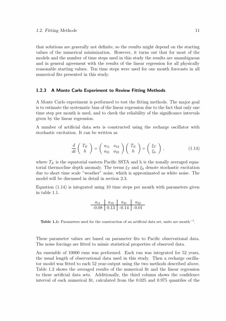
Equation (1.14) is integrated using 10 time steps per month with parameters givenin table 1.1.
a11 a12 a21 a22
-0.08 0.13 -0.14 -0.01
Table 1.1: Parameters used for the construction of an artificial data set, units are month−1.
These parameter values are based on parameter fits to Pacific observational data.The noise forcings are fitted to mimic statistical properties of observed data.
An ensemble of 10000 runs was performed. Each run was integrated for 52 years,the usual length of observational data used in this study. Then a recharge oscilla-tor model was fitted to each 52 year-output using the two methods described above.Table 1.2 shows the averaged results of the numerical fit and the linear regressionto these artificial data sets. Additionally, the third column shows the confidenceinterval of each numerical fit, calculated from the 0.025 and 0.975 quantiles of the
12 CHAPTER 1. DATA AND METHODS
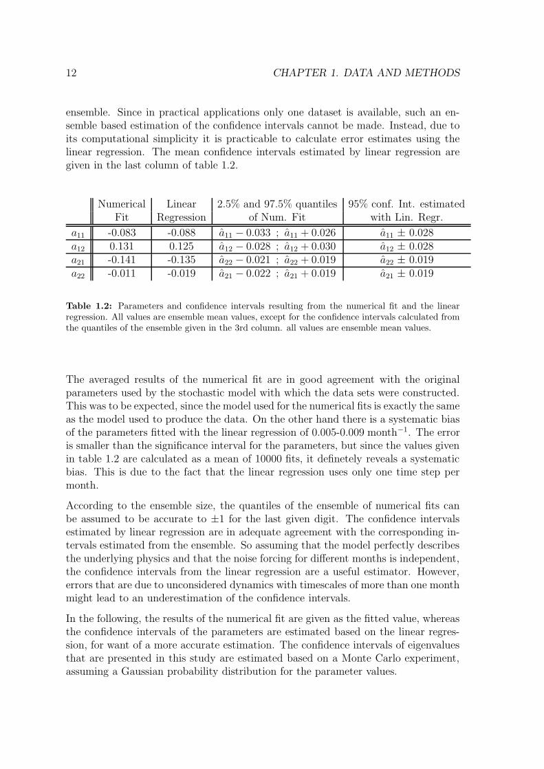
ensemble. Since in practical applications only one dataset is available, such an en-semble based estimation of the confidence intervals cannot be made. Instead, due toits computational simplicity it is practicable to calculate error estimates using thelinear regression. The mean confidence intervals estimated by linear regression aregiven in the last column of table 1.2.
Numerical Linear 2.5% and 97.5% quantiles 95% conf. Int. estimatedFit Regression of Num. Fit with Lin. Regr.
a11 -0.083 -0.088 a11 − 0.033 ; a11 + 0.026 a11 ± 0.028a12 0.131 0.125 a12 − 0.028 ; a12 + 0.030 a12 ± 0.028a21 -0.141 -0.135 a22 − 0.021 ; a22 + 0.019 a22 ± 0.019a22 -0.011 -0.019 a21 − 0.022 ; a21 + 0.019 a21 ± 0.019
Table 1.2: Parameters and confidence intervals resulting from the numerical fit and the linearregression. All values are ensemble mean values, except for the confidence intervals calculated fromthe quantiles of the ensemble given in the 3rd column. all values are ensemble mean values.
The averaged results of the numerical fit are in good agreement with the originalparameters used by the stochastic model with which the data sets were constructed.This was to be expected, since the model used for the numerical fits is exactly the sameas the model used to produce the data. On the other hand there is a systematic biasof the parameters fitted with the linear regression of 0.005-0.009 month−1. The erroris smaller than the significance interval for the parameters, but since the values givenin table 1.2 are calculated as a mean of 10000 fits, it definetely reveals a systematicbias. This is due to the fact that the linear regression uses only one time step permonth.
According to the ensemble size, the quantiles of the ensemble of numerical fits canbe assumed to be accurate to ±1 for the last given digit. The confidence intervalsestimated by linear regression are in adequate agreement with the corresponding in-tervals estimated from the ensemble. So assuming that the model perfectly describesthe underlying physics and that the noise forcing for different months is independent,the confidence intervals from the linear regression are a useful estimator. However,errors that are due to unconsidered dynamics with timescales of more than one monthmight lead to an underestimation of the confidence intervals.
In the following, the results of the numerical fit are given as the fitted value, whereasthe confidence intervals of the parameters are estimated based on the linear regres-sion, for want of a more accurate estimation. The confidence intervals of eigenvaluesthat are presented in this study are estimated based on a Monte Carlo experiment,assuming a Gaussian probability distribution for the parameter values.
1.2. Fitting Methods 13
1.2.4 Seasonal Dependent Parameter Fits
For some models presented in the following, seasonal dependent parameter sets shallbe fitted. However, if parameters are fitted separately for each calendar month theeffective sample size is only one twelfth of the sample size available for non-seasonal-dependent fits. To attain maximum sample size retaining maximum seasonal resolu-tion, a 3 month moving data block is used to fit monthly parameters. This meansthat parameters for a calendar month m are fitted using data of the calendar monthsm-1, m, and m+1 modulo 12. For example, for the January parameter-values all dataof December, January and February is used for the parameter fit. For the Februaryparameters, January, February and March data is used and so forth.3
3Strictly speaking the predictor data set is formed of data containing months (m-1, m,m+1)mod12. The response variable for month t is constructed as Yt = Xt+1 − Xt.
Chapter 2
Simple Models for ENSO
2.1 Introduction
Our understanding of the coupled atmosphere-ocean dynamics in the tropical Pa-cific, responsible for the well known El Nino events, began with the results of Bjerk-nes (1964). He discovered the positive feedback mechanism between eastern PacificSSTA, zonal wind stress anomalies and ocean dynamics. However, for the observedquasi-periodic development and decay of ENSO anomalies a delayed negative feed-back is also necessary. An early model study of the dynamics resposible for ENSOwas performed by Zebiak and Cane (1987). They were able to reproduce the irreg-ular recurrence of warm events with a preferred period of three to four years in acoupled model of intermediate complexity (ICM). To improve the understanding ofthe basic mechanisms responsible for ENSO, even more simple conceptual modelswere proposed that condense the dynamics to ordinary differential equations (ODE)or delay differential equations (DDE). This class of ENSO models defines the scopeof this study.
Suarez and Schopf (1988) first presented the delayed action oscillator, consisting ofone DDE for eastern equatorial Pacific SSTA. The oscillation in this model is ex-plained by equatorial wave transport processes. A positive (negative) SSTA in theequatorial eastern Pacific induces a positive (negative) zonal wind stress anomalyin the central Pacific. This causes downwelling (upwelling) Kelvin waves travellingto the East and upwelling (downwelling) Rossby waves travelling to the West. TheKelvin waves are therefore responsible for a downwelling (upwelling) in the easternbasin which in turn causes a warming (cooling) of SST. This is the positive Bjerknesfeedback. The oscillation is due to the reflection of the Rossby waves at the westernboundary into upwelling (downwelling) Kelvin waves, inducing the transition to a LaNina (El Nino) event. The SSTA is assumed to be in equilibrium with thermoclinedepth anomalies in this model. Battisti and Hirst (1989) (hereinafter BH89) findthe same equation by following a more strict derivation. They suggest quite differ-
14
2.1. Introduction 15
ent parameter sets, though, corresponding to different regimes, as will be shown inthe next section. More generally, lively discussion exists whether ENSO reveals aself-sustained and irregular behaviour due to nonlinear dynamics within the ”slow”components of the coupled system, whether the oscillation is sustained by uncou-pled short timescale ”weather noise”, or whether the oscillation is self-sustained butthe irregularity is due to the ”weather noise” (see Neelin et al. (1998) an referencestherein).
Jin (1997) proposes the recharge oscillator model, which can be written in terms oftwo linear first order ODEs for eastern Pacific SSTA and thermocline depth anomaly.The oscillation in this model is explained by discharging (recharging) of equatorialheat content during an El Nino (La Nina) event. Equatorial wave travel times arenot explicitly considered in this model. Burgers et al. (2005) perfom a parameter fitof the recharge oscillator model to observational SST and thermocline depth data.Based on the results of their fit they suggest a further simplification of the rechargeoscillator model to a simple damped harmonic oscillator with SSTA playing the roleof momentum and thermocline depth playing the role of position.
One of the shortcomings of all these models is that they do not reproduce the observedkurtosis and skewness of eastern Pacific SSTA, with extreme events being more likelythan for an ordinary Gaussian distribution and El Nino events being stronger thanLa Nina events.
It has been known for long that ENSO is strongly locked to the seasonal cycle, withEl Nino events usually peaking towards the end of the year - after all, El Nino owesits name to this fact. Jin et al. (1996) also discuss a possible influence of seasonalityon ENSO periodicity and its regularity via frequency locking to rational multiples ofone year. They find a quasi-biennial and a 4
3-year peak next to the dominating 4-year
period, in an ICM if the annual cycle is included. The predictability of ENSO doesalso largely depend on the time of the year, with the prominent prediction barrier inboreal spring (e.g. McPhaden (2003)). However, controversial discussion exists onwhether the explicit consideration of seasonality in simple statistical ENSO predictionmodels allows for better forecasts (see for example Xue et al. (2000) and referencestherein).
In this study, the parameters of different conceptual models for ENSO, accountingfor different physical key mechanisms, are fitted to observational data. The differentmodels are then compared in terms of their capability to reproduce observed statisti-cal properties of ENSO, if excited by stochastic forcing, representing short timescaleuncoupled ”weather-noise”. Further their predictive skills as forecast models areexamined.
Sections 2.2 to 2.4 discuss the delayed action oscillator and the recharge oscillatormodel. In section 2.5, a simple unification of the delayed action oscillator and therecharge oscillator is proposed.
16 CHAPTER 2. SIMPLE MODELS FOR ENSO
The observed skewness and kurtosis of Nino3 SSTA timeseries is explained by thenonlinear coupling of SSTA on thermocline depth anomalies and effects of seasonalityin section 2.6.
In section 2.7, seasonality is included in the recharge oscillator model by allowingfor seasonal dependent parameters. It is analyzed whether the observed seasonalitycan be reproduced by such a model and whether the annual mean statistics areinfluenced by the locking to the seasonal cycle. Finally the predictive skill of theseasonal dependent recharge oscillator is examined.
2.2 The Delayed Action Oscillator
2.2.1 Model Description
The ”oldest” conceptual model being discussed in this study is the delayed actionoscillator that was first presented by Suarez and Schopf (1988) and BH89. The linearversion of the delayed oscillator model can be written as
dT
dt(t) = −bT (t − τ) + cT (t) . (2.1)
The equation describes the SST anomaly (T ) averaged over a box in the easternequatorial Pacific which is influenced by a fast feedback represented by cT (t) anda delayed effect represented by the term bT (t − τ). The term cT (t) includes theeffects of thermal damping, upwelling/downwelling Kelvin waves, coastal upwellingand horizontal advection. The term bT (t−τ) accounts for the effects of Rossby wavesreflected as Kelvin waves at the western boundary. τ is thus given by the travel timesof equatorial waves and is estimated to be 180 days in BH89.
It should be stressed that for the parameters proposed by both groups the linearmodel reveals infinite growth. Thus a nonlinear extension is necessary to avoid infinitegrowth.
Using the approach T = T0 exp(λt) for (2.1) the eigenvalues λ are given by theimplicit equation
λ = −b exp(−λτ) + c . (2.2)
The solutions of 2.2 are discussed in detail in BH89. Here, a simple way to approxi-mate the delayed oscillator shall be presented.
The slowly oscillating weakly damped/growing solutions where |λ| << τ−1 (τ is
2.2. The Delayed Action Oscillator 17
estimated to be 180 days here whereas the El Nino period seems to be about 4 years)can be found by approximating T (t − τ) by its Taylor expansion:
T (t − τ) = T (t) − dT
dtτ +
1
2
d2T
dt2τ 2 + O(τ 3) . (2.3)
Therefore, neglecting third and higher order terms, equation (2.1) can be approxi-mated as
dT
dt= −b(T − τ
dT
dt+
τ 2
2
d2T
dt2) + cT . (2.4)
This can be rewritten in the classical form of a damped harmonic oscillator
d2T
dt2= −ω2
0T − 2γdT
dtwith ω2
0 =2(b − c)
bτ 2and γ =
1 − bτ
bτ 2. (2.5)
The eigenvalues of (2.5) are given by
λ1/2 = −γ ±√
γ2 − ω20 . (2.6)
These eigenvalues can be obtained by using the approach T = T0 exp(λt) and solving(2.5) for λ or by rewriting (2.5) into a system of two first order ODEs and calculatingthe eigenvalues of the matrix describing the time derivation, as explained in appendixA. It should be noted that the same solution as in (2.6) is obtained if the exponentialfunction in (2.2) is replaced by its Taylor expansion up to the order τ 2. Equation(2.2), however, has multiple solutions. The general solution of (2.1) is given by aninfinite sum of sinusoidal solutions and is thus generally not exactly sinusoidal itself.Equation (2.6) provides an approximation for the ”slowest” mode, which turns outto be dominant.
It shall especially be pointed out here that the original model described by equation(2.1) as well as the approximation given by (2.5) both reveal a similar division intofour different parameter regimes. The four regimes and the corresponding parameterranges in equation (2.5) are given as1:
Damped solutions for γ > 0 and γ2 > ω20
Damped oscillatory solutions for γ > 0 and γ2 < ω20
Growing oscillatory solutions for γ < 0 and γ2 < ω20
At least 1 purely growing solution for γ < 0 and γ2 > ω20
1Strictly speaking this is only valid if ω20 is positive. If ω2
0 is negative, there is always a purelygrowing mode.
18 CHAPTER 2. SIMPLE MODELS FOR ENSO
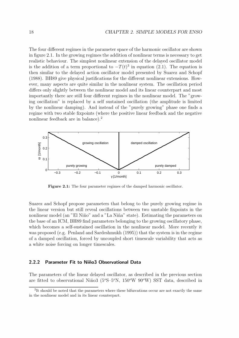
The four different regimes in the parameter space of the harmonic oscillator are shownin figure 2.1. In the growing regimes the addition of nonlinear terms is necessary to getrealistic behaviour. The simplest nonlinear extension of the delayed oscillator modelis the addition of a term proportional to −T (t)3 in equation (2.1). The equation isthen similar to the delayed action oscillator model presented by Suarez and Schopf(1988). BH89 give physical justifications for the different nonlinear extensions. How-ever, many aspects are quite similar in the nonlinear system. The oscillation perioddiffers only slightly between the nonlinear model and its linear counterpart and mostimportantly there are still four different regimes in the nonlinear model. The ”grow-ing oscillation” is replaced by a self sustained oscillation (the amplitude is limitedby the nonlinear damping). And instead of the ”purely growing” phase one finds aregime with two stable fixpoints (where the positive linear feedback and the negativenonlinear feedback are in balance).2
−0.3 −0.2 −0.1 0 0.1 0.2 0.30
0.1
0.2
0.3
γ [1/month]
ω [
1/m
onth
]
purely growing purely damped
growing oscillation damped oscillation
Figure 2.1: The four parameter regimes of the damped harmonic oscillator.
Suarez and Schopf propose parameters that belong to the purely growing regime inthe linear version but still reveal oscillations between two unstable fixpoints in thenonlinear model (an ”El Nino” and a ”La Nina” state). Estimating the parameters onthe base of an ICM, BH89 find parameters belonging to the growing oscillatory phase,which becomes a self-sustained oscillation in the nonlinear model. More recently itwas proposed (e.g. Penland and Sardeshmukh (1995)) that the system is in the regimeof a damped oscillation, forced by uncoupled short timescale variability that acts asa white noise forcing on longer timescales.
2.2.2 Parameter Fit to Nino3 Observational Data
The parameters of the linear delayed oscillator, as described in the previous sectionare fitted to observational Nino3 (5oS–5oN, 150oW 90oW) SST data, described in
2It should be noted that the parameters where these bifurcations occur are not exactly the samein the nonlinear model and in its linear counterpart.
2.2. The Delayed Action Oscillator 19
section 1.1, by minimizing the rms error of one month forecasts. The fit routines aredescribed in section 1.2.
Parameters and prediction skills are cross-validated by first using the time periodfrom 1950 to 1975 for the parameter fit and the period from 1976 to 2001 for theevaluation of the forecast skill and vice versa.
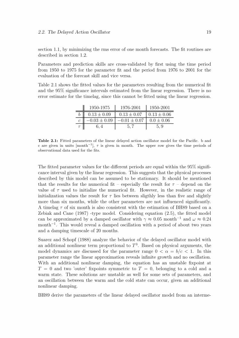
Table 2.1 shows the fitted values for the parameters resulting from the numerical fitand the 95% significance intervals estimated from the linear regression. There is noerror estimate for the timelag, since this cannot be fitted using the linear regression.
1950-1975 1976-2001 1950-2001
b 0.13 ± 0.09 0.13 ± 0.07 0.13 ± 0.06c −0.03 ± 0.09 −0.01 ± 0.07 0.0 ± 0.06τ 6, 4 5, 7 5, 9
Table 2.1: Fitted parameters of the linear delayed action oscillator model for the Pacific. b andc are given in units [month−1], τ is given in month. The upper row gives the time periods ofobservational data used for the fits.
The fitted parameter values for the different periods are equal within the 95% signifi-cance interval given by the linear regression. This suggests that the physical processesdescribed by this model can be assumed to be stationary. It should be mentionedthat the results for the numerical fit – especially the result for τ – depend on thevalue of τ used to initialize the numerical fit. However, in the realistic range ofinitialization values the result for τ lies between sligthly less than five and slightlymore than six months, while the other parameters are not influenced significantly.A timelag τ of six month is also consistent with the estimation of BH89 based on aZebiak and Cane (1987) -type model. Considering equation (2.5), the fitted modelcan be approximated by a damped oscillator with γ ≈ 0.05 month−1 and ω ≈ 0.24month−1. This would reveal a damped oscillation with a period of about two yearsand a damping timescale of 20 months.
Suarez and Schopf (1988) analyze the behavior of the delayed oscillator model withan additional nonlinear term proportional to T 3. Based on physical arguments, themodel dynamics are discussed for the parameter range 0 < α = b/c < 1. In thisparameter range the linear approximation reveals infinite growth and no oscillation.With an additional nonlinear damping, the equation has an unstable fixpoint atT = 0 and two ’outer’ fixpoints symmetric to T = 0, belonging to a cold and awarm state. These solutions are unstable as well for some sets of parameters, andan oscillation between the warm and the cold state can occur, given an additionalnonlinear damping.
BH89 derive the parameters of the linear delayed oscillator model from an interme-
20 CHAPTER 2. SIMPLE MODELS FOR ENSO
diate complex coupled model. They find parameters b = 3.9 yr−1 ' 0.33 month−1,c = 2.2 yr−1 ' 0.18 month−1 and τ = 180 days' 6 months. In this parameter rangethe model reveals a growing oscillation with a dominating period of 3 years. This isin good agreement with the intermediate complex model that is used to derive theseparameters, which also reveals a growing oscillation in its linearized approximation.
The fits performed in this study suggest a damped oscillatory parameter regime. Toexclude the possibility that the linear damping/amplification c is underestimated,due to the lack of an explicit consideration of a nonlinear damping, parameter fitswith an additional term proportional to T 3 were also performed. In contrast to theassumptions of Suarez and Schopf (1988) and BH89 that the linear approximationreveals a purely growing or growing oscillatory mode, which is damped by nonlineareffects, the nonlinear parameter fit results in a linear damping (i.e. c < 0) andno significant nonlinear damping or amplification3. For this reason this nonlinearextension is not discussed in more detail here.
2 4 6 8 10 120
0.2
0.4
0.6
0.8
1SST Correlation
lead month2 4 6 8 10 12
0
0.2
0.4
0.6
0.8
1
1.2
lead month
stan
dard
dev
iatio
n
SST RMS−error
1976−2001
1976−2001 Damped Persist.
1950−1975
1950−1975 Damped Persist.
1950−2001
1950−2001 Damped Perst.
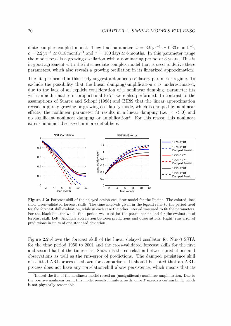
Figure 2.2: Forecast skill of the delayed action oscillator model for the Pacific. The colored linesshow cross-validated forecast skills. The time intervals given in the legend refer to the period usedfor the forecast skill evaluation, while in each case the other interval was used to fit the parameters.For the black line the whole time period was used for the parameter fit and for the evaluation offorecast skill. Left: Anomaly correlation between predictions and observations. Right: rms error ofpredictions in units of one standard deviation.
Figure 2.2 shows the forecast skill of the linear delayed oscillator for Nino3 SSTAfor the time period 1950 to 2001 and the cross-validated forecast skills for the firstand second half of the timeseries. Shown is the correlation between predictions andobservations as well as the rms-error of predictions. The damped persistence skillof a fitted AR1-process is shown for comparison. It should be noted that an AR1-process does not have any correlation-skill above persistence, which means that its
3Indeed the fits of the nonlinear model reveal an (unsignificant) nonlinear amplification. Due tothe positive nonlinear term, this model reveals infinite growth, once T exeeds a certain limit, whichis not physically reasonable.
2.2. The Delayed Action Oscillator 21
correlation skill is simply the auto-correlation of the timeseries. On the other hand,the rms-error of (undamped) persistence forecasts, which converges towards
√2 times
the standard deviation, is always higher than the rms-error of an AR1-process, whichconverges towards one standard deviation for long lead times. This should also bekept in mind if the forecast skill of a GCM is compared to any damped model or toensemble predictions. While the rms-error of single GCM runs also converges towards√
2 times the standard deviation for long ”unpredictable” lead times, the skill of anydamped model or of a large ensemble mean converges towards one standard deviation.They will therefore naturally have a smaller rms-error, especially for long lead times,than a single GCM run even if this is not the case for the correlation skill, which issometimes not clearly pointed out in literature.
Significant forecast skill above damped persistence is found for both cross-validatedtimeseries using the delayed action oscillator model. The small difference betweenthe cross-validated skills and the skill of the not cross-validated run using the wholetimeseries for the parameter fits and for the evaluation suggests that 26 years providesufficient data for the fits and that there is very little artificial skill.
2.2.3 The Delayed Oscillator Excited by Stochastic Forcing
With the parameters fitted in the previous section, the model reveals damped os-cillatory behaviour. To retain variance the model, which shows damped oscillatorybehaviour for the parameters fitted in the previous section, is excited by stochasticexitation as proposed for example by Jin (1997) for the recharge oscillator model.Physically, the noise forcing represents short timescale uncoupled variability, that isassumed to be representable by white noise forcing on the timescales of the coupledatmosphere-ocean dynamics described by the model (see also Hasselmann (1976)).The equation for the delayed oscillator excited by stochastic forcing can then bewritten as
dT
dt(t) = −bT (t − τ) + cT (t) + ξ(t) , (2.7)
where ξ(t) represents the white noise forcing.
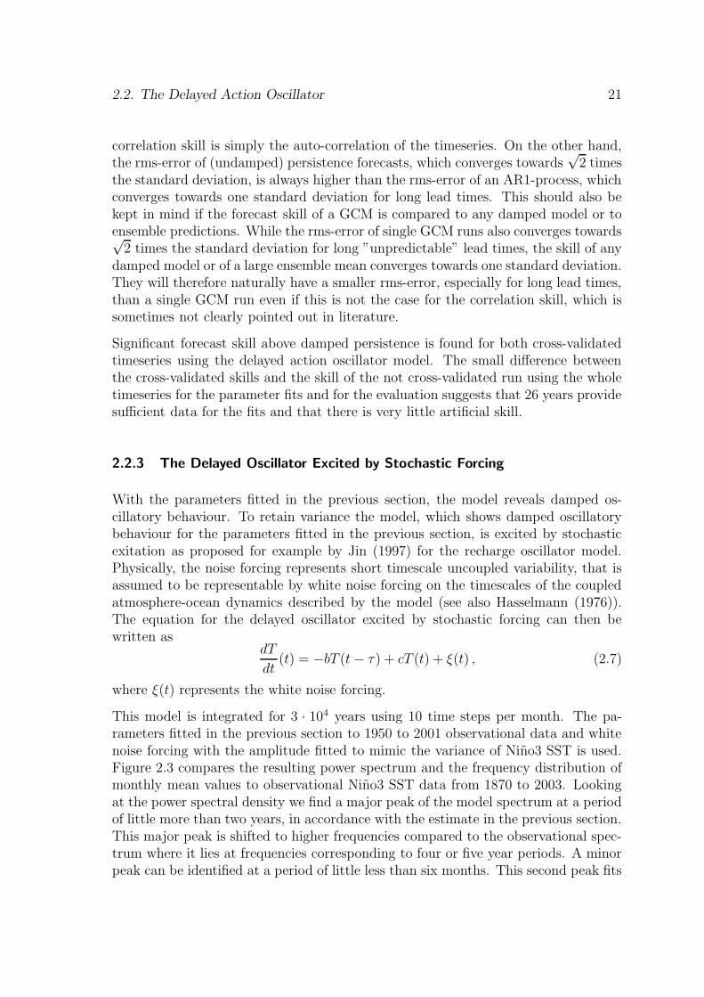
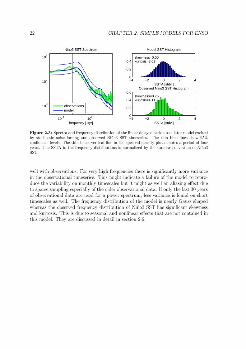
This model is integrated for 3 · 104 years using 10 time steps per month. The pa-rameters fitted in the previous section to 1950 to 2001 observational data and whitenoise forcing with the amplitude fitted to mimic the variance of Nino3 SST is used.Figure 2.3 compares the resulting power spectrum and the frequency distribution ofmonthly mean values to observational Nino3 SST data from 1870 to 2003. Lookingat the power spectral density we find a major peak of the model spectrum at a periodof little more than two years, in accordance with the estimate in the previous section.This major peak is shifted to higher frequencies compared to the observational spec-trum where it lies at frequencies corresponding to four or five year periods. A minorpeak can be identified at a period of little less than six months. This second peak fits
22 CHAPTER 2. SIMPLE MODELS FOR ENSO
10−1
100
10−2
100
102
frequency [1/yr]
Nino3 SST Spectrum
observationsmodel
−4 −2 0 2 40
0.2
0.4skewness=0.00kurtosis=3.02
Model SST Histogram
SSTA [stdv.]
−4 −2 0 2 40
0.2
0.4
0.6skewness=0.76kurtosis=4.11
Observed Nino3 SST Histogram
SSTA [stdv.]
Figure 2.3: Spectra and frequency distribution of the linear delayed action oscillator model excitedby stochastic noise forcing and observed Nino3 SST timeseries. The thin blue lines show 95%confidence levels. The thin black vertical line in the spectral density plot denotes a period of fouryears. The SSTA in the frequency distributions is normalized by the standard deviation of Nino3SST.
well with observations. For very high frequencies there is significantly more variancein the observational timeseries. This might indicate a failure of the model to repro-duce the variability on monthly timescales but it might as well an aliasing effect dueto sparse sampling especially of the older observational data. If only the last 30 yearsof observational data are used for a power spectrum, less variance is found on shorttimescales as well. The frequency distribution of the model is nearly Gauss shapedwhereas the observed frequency distribution of Nino3 SST has significant skewnessand kurtosis. This is due to seasonal and nonlinear effects that are not contained inthis model. They are discussed in detail in section 2.6.
2.3. The Recharge Oscillator 23
2.3 The Recharge Oscillator
2.3.1 Model Description
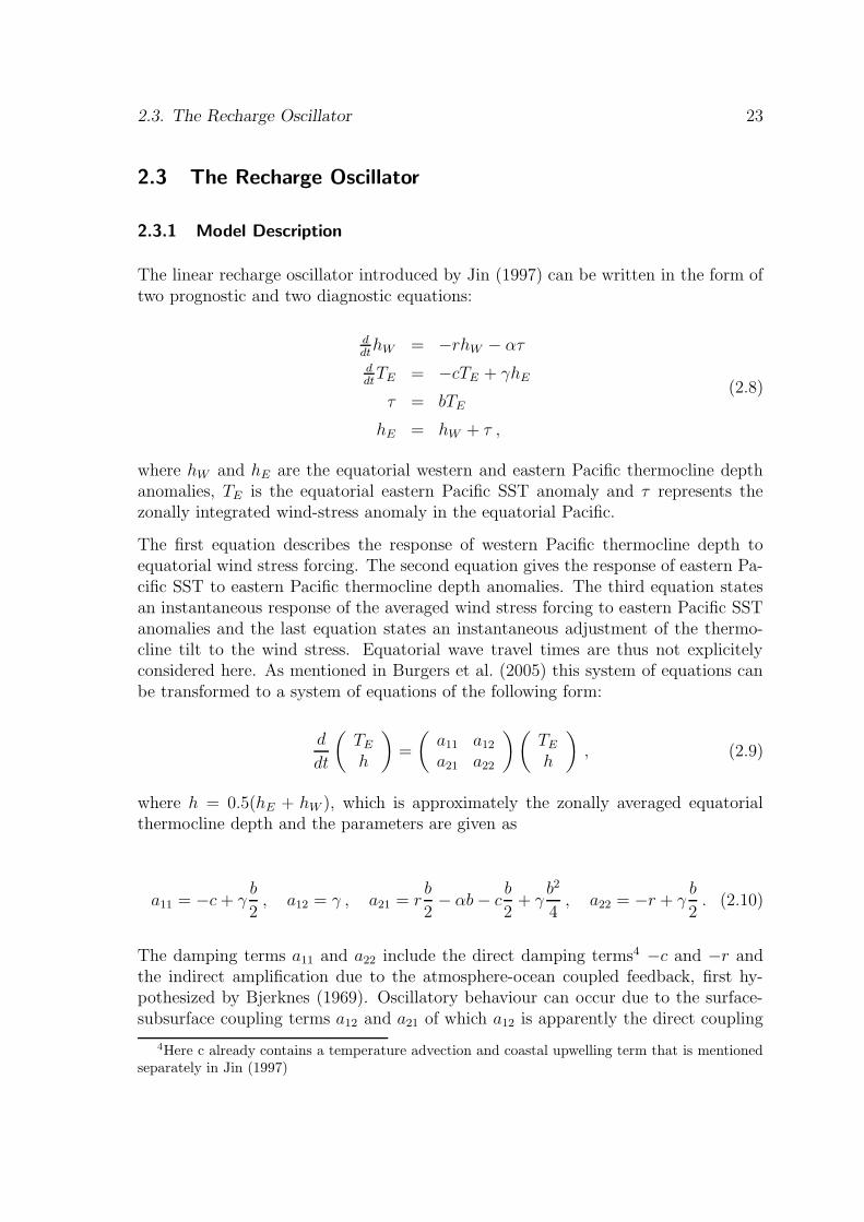
The linear recharge oscillator introduced by Jin (1997) can be written in the form oftwo prognostic and two diagnostic equations:
ddt
hW = −rhW − ατddt
TE = −cTE + γhE
τ = bTE
hE = hW + τ ,
(2.8)
where hW and hE are the equatorial western and eastern Pacific thermocline depthanomalies, TE is the equatorial eastern Pacific SST anomaly and τ represents thezonally integrated wind-stress anomaly in the equatorial Pacific.
The first equation describes the response of western Pacific thermocline depth toequatorial wind stress forcing. The second equation gives the response of eastern Pa-cific SST to eastern Pacific thermocline depth anomalies. The third equation statesan instantaneous response of the averaged wind stress forcing to eastern Pacific SSTanomalies and the last equation states an instantaneous adjustment of the thermo-cline tilt to the wind stress. Equatorial wave travel times are thus not explicitelyconsidered here. As mentioned in Burgers et al. (2005) this system of equations canbe transformed to a system of equations of the following form:
d
dt
(
TE
h
)
=
(
a11 a12
a21 a22
)(
TE
h
)
, (2.9)
where h = 0.5(hE + hW ), which is approximately the zonally averaged equatorialthermocline depth and the parameters are given as
a11 = −c + γb
2, a12 = γ , a21 = r
b
2− αb − c
b
2+ γ
b2
4, a22 = −r + γ
b
2. (2.10)
The damping terms a11 and a22 include the direct damping terms4 −c and −r andthe indirect amplification due to the atmosphere-ocean coupled feedback, first hy-pothesized by Bjerknes (1969). Oscillatory behaviour can occur due to the surface-subsurface coupling terms a12 and a21 of which a12 is apparently the direct coupling
4Here c already contains a temperature advection and coastal upwelling term that is mentionedseparately in Jin (1997)

24 CHAPTER 2. SIMPLE MODELS FOR ENSO
of surface temperature to the subsurface watermass that is considered to be relativelywarm when the thermocline is deep, and cold when the thermocline is shallow. Thecoupling of thermocline depth to SST on the other hand is only via the atmosphericbridge as expected, which can be seen by the occurence of b in all terms of a21 in (2.10)and is, as suggested by parameter fits, dominated by the negative terms. This allowsfor the ’recharge mechanism’, which means that the mean thermocline raises and theequatorial heat content discharges during an El Nino event, allowing for the transi-tion to a La Nina, whereas equatorial heat content recharges during a La Nina event,allowing for the transition towards an El Nino. This recharge-discharge mechanismwas shown to be necessary for the El Nino oscillation by Zebiak and Cane (1987) andit is confirmed by analysis of observational data by Meinen and McPhaden (2000).
It should be stressed that equation (2.8) could also be transformed into an equationsimilar to (2.9) with h being replaced by hE or hW and with different parameters aij.The averaged thermocline depth, however, turns out to be a very useful predictorvariable.
Equation (2.9) can be transformed into one second order ODE for TE. Definingγ = −1
2(a11 + a22) and ω2
0 = a11a22 − a12a21, it has the common form of the dampedoscillator equation
d2TE
dt2= −ω2
0TE + 2γdTE
dt. (2.11)
Thus, the discussion of the four parameter regimes in section 2.2 is equally valid forthe recharge oscillator model.
As explained in Appendix A the eigenvalues of the recharge oscillator are given bythe eigenvalues of the matrix in 2.9 as
λ1,2 =1
2(a11 + a22) ±
√
(a11 − a22)2
4+ a12a21 . (2.12)
So the criterion for oscillatory behaviour is
−a12a21 >(a11 − a22)
2
4y (2.13)
and in the oscillatory regime the criterion for growth (what corresponds to a self-sustained oscillation in the nonlinear extension) is given by
a11 + a22 > 0 . (2.14)
2.3. The Recharge Oscillator 25
2.3.2 Parameter Fit to Observational Data
The parameters of the recharge oscillator as written in equation (2.9) are fitted usingHADISST Nino3 SST data for TE and 20oC isotherm GCM data averaged over theequatorial Pacific (120oE 80oW) for h. The data is described in detail in section 1.1and the parameter fits are explained in section 1.2.
Parameters and prediction skills are cross-validated by first using the time periodfrom 1950 to 1975 for the parameter fit and the period from 1976 to 2001 for theevaluation of the forecast skill and vice versa. Additionally a ”best fit” was performedusing the whole data set from 1950 to 2001.
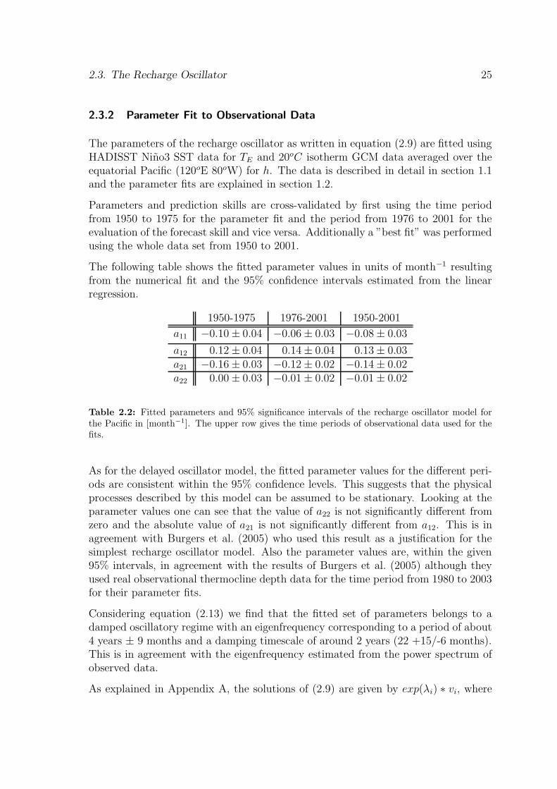
The following table shows the fitted parameter values in units of month−1 resultingfrom the numerical fit and the 95% confidence intervals estimated from the linearregression.
1950-1975 1976-2001 1950-2001
a11 −0.10 ± 0.04 −0.06 ± 0.03 −0.08 ± 0.03
a12 0.12 ± 0.04 0.14 ± 0.04 0.13 ± 0.03a21 −0.16 ± 0.03 −0.12 ± 0.02 −0.14 ± 0.02a22 0.00 ± 0.03 −0.01 ± 0.02 −0.01 ± 0.02
Table 2.2: Fitted parameters and 95% significance intervals of the recharge oscillator model forthe Pacific in [month−1]. The upper row gives the time periods of observational data used for thefits.
As for the delayed oscillator model, the fitted parameter values for the different peri-ods are consistent within the 95% confidence levels. This suggests that the physicalprocesses described by this model can be assumed to be stationary. Looking at theparameter values one can see that the value of a22 is not significantly different fromzero and the absolute value of a21 is not significantly different from a12. This is inagreement with Burgers et al. (2005) who used this result as a justification for thesimplest recharge oscillator model. Also the parameter values are, within the given95% intervals, in agreement with the results of Burgers et al. (2005) although theyused real observational thermocline depth data for the time period from 1980 to 2003for their parameter fits.
Considering equation (2.13) we find that the fitted set of parameters belongs to adamped oscillatory regime with an eigenfrequency corresponding to a period of about4 years ± 9 months and a damping timescale of around 2 years (22 +15/-6 months).This is in agreement with the eigenfrequency estimated from the power spectrum ofobserved data.
As explained in Appendix A, the solutions of (2.9) are given by exp(λi) ∗ vi, where
26 CHAPTER 2. SIMPLE MODELS FOR ENSO
λi are the eigenvalues and vi are the corresponding eigenvectors. If the criterion foroscillation (2.13) is fulfilled, one pair of complex conjugated eigenvalues and eigenvec-tors is found, from which the phase relation of TE and h can be determined. For thefitted parameters thermocline depth anomalies lead SSTA by about 75o, and SSTAlead thermocline depth anomalies of opposite sign by 105o. This phase differencedescribes the heating/cooling of SST due to thermocline depth anomalies and therecharging/discharging of heat content during a La Nina/El Nino event which is es-sential for the oscillation. For an undamped oscillation the phase difference is exactly90o.
0 0.5 1 1.5−0.4
−0.2
0
0.2
0.4
µ
[mon
th−
1 ]
Parameters of the Recharge Oscillator Model from Estimates of Jin (1997) Compared to Fitted Values
a11a12a21a22
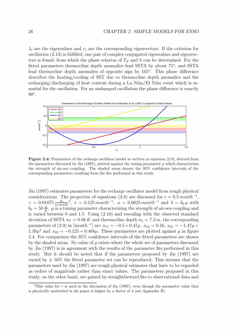
Figure 2.4: Parameters of the recharge oscillator model as written in equation (2.9), derived fromthe parameters discussed by Jin (1997), plotted against the tuning parameter µ which characterizesthe strength of air-sea coupling. The shaded areas denote the 95% confidence intervals of thecorresponding parameters resulting from the fits performed in this study.
Jin (1997) estimates parameters for the recharge oscillator model from rough physicalconsiderations. The properties of equations (2.8) are discussed for c = 0.5 month−1,γ = 0.01875 K
m month5, r = 0.125 month−1, α = 0.0625 month−1 and b = b0 µ with
b0 = 50 mK
. µ is a tuning parameter characterizing the strength of air-sea coupling andis varied between 0 and 1.5. Using (2.10) and rescaling with the observed standarddeviation of SSTA σT = 0.86 K and thermocline depth σh = 7.3 m, the correspondingparameters of (2.9) in [month−1] are a11 = −0.5+0.47µ, a12 = 0.16, a21 = −1.47µ+1.38µ2 and a22 = −0.125 + 0.468µ. These parameters are plotted against µ in figure2.4. For comparison the 95% confidence intervals of the fitted parameters are shownby the shaded areas. No value of µ exists where the whole set of parameters discussedby Jin (1997) is in agreement with the results of the parameter fits performed in thisstudy. But it should be noted that if the parameters proposed by Jin (1997) arevaried by ± 50% the fitted parameter set can be reproduced. This stresses that theparameters used by Jin (1997) are rough physical estimates that have to be regardedas orders of magnitude rather than exact values. The parameters proposed in thisstudy, on the other hand, are gained by straightforward fits to observational data and
5This value for γ is used in the discussion of Jin (1997), even though the parameter value thatis physically motivated in his paper is higher by a factor of 4 (see Appendix B)
2.3. The Recharge Oscillator 27
therefore allow for conclusions about the actual parameter regime describing ENSO.
2 4 6 8 10 120
0.2
0.4
0.6
0.8
1SST Correlation
lead month2 4 6 8 10 12
0
0.20.40.60.8
11.2
1.4SST RMS−error
lead month
stan
dard
dev
iatio
n
2 4 6 8 10 120
0.2
0.4
0.6
0.8
1h Correlation
lead month2 4 6 8 10 12
0
0.20.40.60.8
11.21.4
h RMS−error
lead month
stan
dard
dev
iatio
n
1976−2001
1976−2001 Damped Pers.
1950−1975
1950−1975 Damped Pers.
1950−2001
1950−2001 Damped Pers.
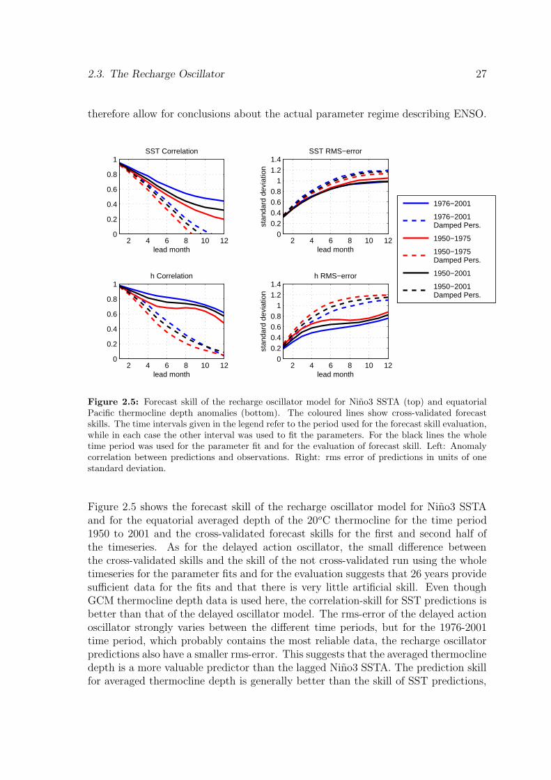
Figure 2.5: Forecast skill of the recharge oscillator model for Nino3 SSTA (top) and equatorialPacific thermocline depth anomalies (bottom). The coloured lines show cross-validated forecastskills. The time intervals given in the legend refer to the period used for the forecast skill evaluation,while in each case the other interval was used to fit the parameters. For the black lines the wholetime period was used for the parameter fit and for the evaluation of forecast skill. Left: Anomalycorrelation between predictions and observations. Right: rms error of predictions in units of onestandard deviation.
Figure 2.5 shows the forecast skill of the recharge oscillator model for Nino3 SSTAand for the equatorial averaged depth of the 20oC thermocline for the time period1950 to 2001 and the cross-validated forecast skills for the first and second half ofthe timeseries. As for the delayed action oscillator, the small difference betweenthe cross-validated skills and the skill of the not cross-validated run using the wholetimeseries for the parameter fits and for the evaluation suggests that 26 years providesufficient data for the fits and that there is very little artificial skill. Even thoughGCM thermocline depth data is used here, the correlation-skill for SST predictions isbetter than that of the delayed oscillator model. The rms-error of the delayed actionoscillator strongly varies between the different time periods, but for the 1976-2001time period, which probably contains the most reliable data, the recharge oscillatorpredictions also have a smaller rms-error. This suggests that the averaged thermoclinedepth is a more valuable predictor than the lagged Nino3 SSTA. The prediction skillfor averaged thermocline depth is generally better than the skill of SST predictions,
28 CHAPTER 2. SIMPLE MODELS FOR ENSO
indicating that the signal in the first is less noisy. It should be stressed, however,that this might be different if real observational data is used for thermocline depth,instead of GCM data.
2.3.3 The Recharge Oscillator Excited by Stochastic Forcing
Analogue to section 2.2.3 the model is excited by stochastic forcing. The major effectsof short timescale weather fluctuations on the eastern Pacific SSTA and averagedheat content are via air temperature variability and via variations of the wind stressforcing, with the first acting on SSTA and the latter acting on both6. The modelwith stochastic excitation can be written as:
d
dt
(
TE
h
)
=
(
a11 a12
a21 a22
)(
TE
h
)
+
(
ξT
ξh
)
(2.15)
where ξT and ξh are the net forcings acting on eastern Pacific SST and averagedthermocline depth. However, as indicated above, ξT and ξh can generally not beassumed to be independent even if wind stress and air temperature anomalies areassumed to be independent.
Assuming that ξT and ξh are correlated in phase, which means that the cross spectraldensity PξT ξh
is real, the power spectral density of SST and thermocline depth forthe model given by equations (2.15) can be calculated analytically as7
PTT (ω) =a2
12Pξhξh+ (ω2 + a2
22)PξT ξT− 2a12a22PξhξT
(ω2 + a12a21 − a11a22)2 + (a11 + a22)2ω2(2.16)
and
Phh(ω) =a2
21PξT ξT+ (ω2 + a2
11)Pξhξh− 2a21a11PξhξT
(ω2 + a12a21 − a11a22)2 + (a11 + a22)2ω2. (2.17)
Since a12a22 < 0 while a21a11 > 0 it can be seen that a positive correlation betweenξh and ξT increases the variance of T while it decreases the variance of h. Foruncorrelated forcing the total variance of h is too high compared to observations forany finite variance of ξh. Thus a correlation between the two noise forcings of 0.32(corresponding to 10% explained variance) is chosen for the following experiments,to mimic the total variance of observed Nino3 SST and averaged thermocline depthwith still a reasonable amount of noise on the thermocline depth. The variances ofthe noise forcings meet σξT
= 1.5 σξh. The choice of the correlation and the total
6Since the thermocline tilt is assumed to be in equilibrium with the wind stress in this model,there is also quite a large effect of wind stress forcing on eastern Pacific SSTA.
7Regard appendix C for a cautionary note on the definition of spectra for processes continuousin time.
2.3. The Recharge Oscillator 29
variance of the noise forcings is somewhat arbitrary, since three degrees of freedom(σξT
, σξhand the correlation) exist while only the two total variances of T and h are
fitted to observations. However, the qualitative results presented in the following arenot altered if the correlations and variances are chosen in a reasonable range.
10−1
100
10−2
10−1
100
101
102
frequency [1/yr]
Nino3 SST Spectrum
observations (1870−2003)
model
10−1
100
10−2
10−1
100
101
102
frequency [1/yr]
Thermocline Depth Spectrum
GCM−data (1950−2001)
BMRC−Obs. (1980−2005)
model
−4 −2 0 2 40
0.2
0.4
0.6skewness=0.02
kurtosis=3.04
Model SST Histogram
SSTA [stdv.]
−4 −2 0 2 40
0.2
0.4
0.6skewness=0.76
kurtosis=4.11
Observed Nino3 SST Histogram
SSTA [stdv.]
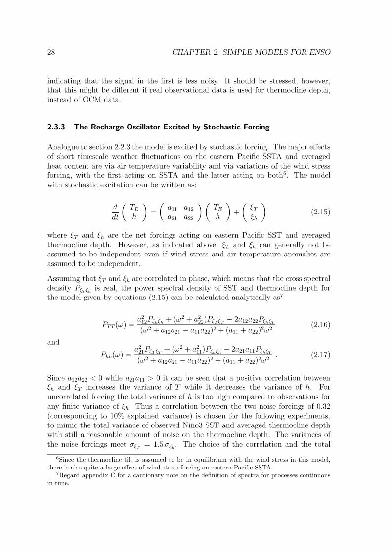
Figure 2.6: Left: Power spectral density of eastern Pacific SST time series from the rechargeoscillator model compared to observed Nino3 SST data. The thin blue lines denote 95% confidencelevels. The thin vertical line denotes a period of four years. Center: The same for the modelthermocline depth and 20oC isotherm depth from a GCM run forced with NCEP data and fromBMRC observational data. The thin blue lines show 95% confidence levels based on the time periodof the GCM data. Right: Nino3 SSTA frequency distribution of the recharge oscillator model (top)and from observations (bottom). The SSTA is normalized by the standard deviation of Nino3 SST.
Figure 2.6 shows the model power spectra, calculated from equations (2.16) and(2.17) as well as the SST frequency distribution resulting from a numerical 3 · 104
year model integration similar to section 2.2.3. The model SST spectrum fits well withobservations, especially on longer timescales. However, the minor peak at a period ofabout 6 months, that can be identified in the observational spectrum and that wasreproduced by the delayed oscillator model, is naturally not included in the rechargeoscillator model, since the latter describes a damped harmonic oscillation. The highvariance on the high frequency end of the spectrum of the observed timeseries hasalready been discussed in section 2.2.3. The spectrum of the model thermoclinedepth timeseries has a too pronounced peak at the El Nino period and too muchvariance on shorter timescales compared to the NCEP forced GCM data. The realobservational BMRC timeseries on the other hand shows a more pronounced peakand more variance on shorter timescales as well. Generally, differences are hardlysignificant and statements about the observational thermocline depth spectrum arevery speculative since too little data exists. As for the delayed oscillator, the frequencydistribution of the model SST is, unlike the observations, nearly Gauss shaped. Forfurther discussion about the reasons for skewness and kurtosis in the observed Nino3
30 CHAPTER 2. SIMPLE MODELS FOR ENSO
timeseries see section 2.6.
−20 −15 −10 −5 0 5 10 15 20−0.8−0.7−0.6−0.5−0.4−0.3−0.2−0.1
00.10.20.30.40.50.60.70.8
Cross Correlation T vs h
h leads T T leads h
observationsmodel
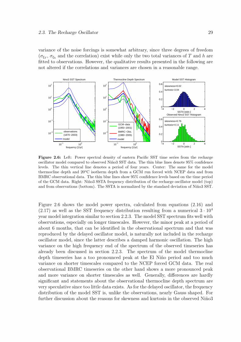
Figure 2.7: Cross correlation between Nino3 SSTA and thermocline depth anomalies averaged overthe equatorial Pacific from 1950 to 2001 observational/forced GCM data (green) compared to theresults of the recharge oscillator model (blue). Correlations above 0.27 a significant on are 95% levelassuming 52 degrees of freedom, for the observational data.
Figure 2.7 shows the cross-correlation between Nino3 SSTA (T ) and thermoclinedepth anomalies averaged over the equatorial Pacific (h) from the recharge oscillatormodel integration, compared to observational/forced GCM data. The observed cross-correlation has maxima with thermocline depth anomalies leading SSTA by about6 months and with SSTA leading thermocline depth anomalies of opposite sign byabout 9 months. The first describes the coupling of SSTA on thermocline depthanomalies while the second describes the recharging (discharging) of equatorial heatcontent during a La Nina (El Nino) event. These are the key mechanisms responsiblefor the oscillation in the recharge oscillator picture. Further, this correlations explainthe relevance of averaged thermocline depth as a predictor for Nino3 SSTA and viceversa. The cross-correlation is generally reproduced well by the recharge oscillatormodel, even though correlations for long lead times tend to be too high. Especially,the recharge oscillator model reaches a maximum correlation slightly above 0.6 forthermocline depth leading SSTA by about 9 months, while the maximum is reachedfor thermocline depth leading SSTA by only about 6 months and is beneath 0.5 inthe observational/forced GCM data.
2.4 The Simplest Recharge Oscillator
Burgers et al. (2005) suggest that the recharge oscillator model described above canagain be simplified. They fit the recharge oscillator model to observational datafinding that if Nino3 SST and equatorial averaged thermocline depth time series are
2.4. The Simplest Recharge Oscillator 31
normalized by their standard deviation the damping of thermocline depth a22 can beneglected and the surface-subsurface coupling parameters a12 and a21 can assumedto be equal. This is supported by the parameter fits presented in section 2.3. Therecharge oscillator model can thus be simplified to
d
dt
(
TE
h
)
=
(
−2γ ω0
−ω0 0
)(
TE
h
)
(2.18)
which has the same form as the equation of a damped harmonic oscillator with hplaying the role of position and TE playing the role of momentum.
It should be stressed that the justification for this simplification of the rechargeoscillator model is based on the results of parameter fits only and is not legitimatedphysically in any way.
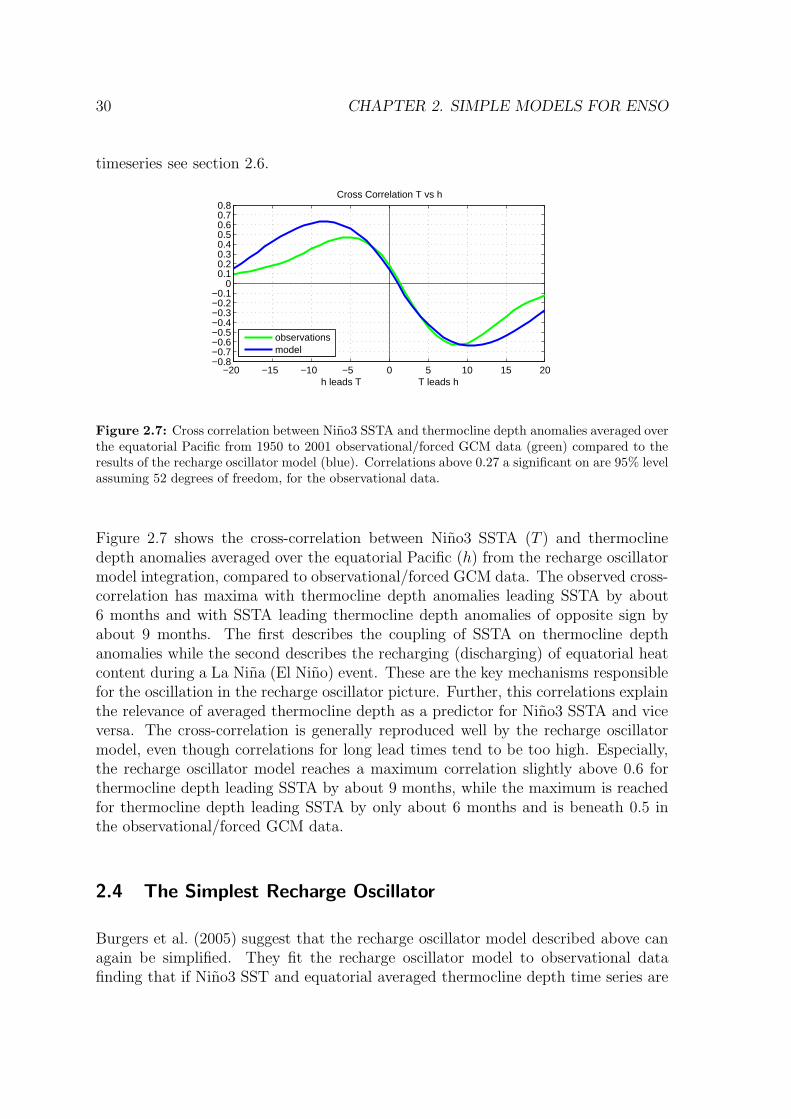
A parameter fit for the simplest recharge oscillator as suggested in equation (2.18) isperformed using the same data as for the recharge oscillator model in the previoussection. The fitting methods are described in section 1.2. Table 2.3 shows the fit-ted parameter values resulting from the numerical fit and the 95% confidence levelsestimated from the linear regression.
1950-1975 1976-2001 1950-2001
γ 0.055 ± 0.018 0.030 ± 0.013 0.040 ± 0.011ω0 0.140 ± 0.024 0.131 ± 0.020 0.133 ± 0.015
Table 2.3: Fitted parameters and 95% confidence levels of the simplest recharge oscillator modelfor the Pacific in [month−1]. The upper row gives the time periods of observational data used forthe fits.
If γ is compared to 12a11 and ω0 is compared to a12 and a21 in the recharge oscillator,
it is found that these results are in good agreement with the parameter fits of section2.3.2. However, the error estimates are smaller than those for the recharge oscillatormodel, which reflects the fact that this model includes only half as much parame-ters. The forecast skill of this model (not shown) is identical to that of the rechargeoscillator model. Expectedly the statistical properties of the simplest recharge oscil-lator model (not shown) forced by stochastic excitation do not show any significantdifferences to the recharge oscillator model presented in the previous section.
32 CHAPTER 2. SIMPLE MODELS FOR ENSO
2.5 The Delayed Recharge Oscillator
2.5.1 Model Description
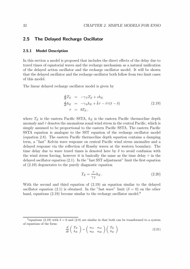
In this section a model is proposed that includes the direct effects of the delay due totravel times of equatorial waves and the recharge mechanism as a natural unificationof the delayed action oscillator and the recharge oscillator model. It will be shownthat the delayed oscillator and the recharge oscillator both follow from two limit casesof this model.
The linear delayed recharge oscillator model is given by
ddt
TE = −γTTE + chE
ddt
hE = −γhhE + kτ − rτ(t − δ)
τ = bTE ,
(2.19)
where TE is the eastern Pacific SSTA, hE is the eastern Pacific thermocline depthanomaly and τ denotes the anomalous zonal wind stress in the central Pacific, which issimply assumed to be proportional to the eastern Pacific SSTA. The eastern PacificSSTA equation is analogue to the SST equation of the recharge oscillator model(equation 2.8). The eastern Pacific thermocline depth equation contains a dampingterm, a ”fast” Kelvin wave response on central Pacific wind stress anomalies and adelayed response via the reflection of Rossby waves at the western boundary. Thetime delay due to wave travel times is denoted here by δ to avoid confusion withthe wind stress forcing, however it is basically the same as the time delay τ in thedelayed oscillator equation (2.1). In the ”fast SST adjustment” limit the first equationof (2.19) degenerates to the purely diagnostic equation
TE =c
γThE . (2.20)
With the second and third equation of (2.19) an equation similar to the delayedoscillator equation (2.1) is obtained. In the ”fast wave” limit (δ = 0) on the otherhand, equations (2.19) become similar to the recharge oscillator model.8
8equations (2.19) with δ = 0 and (2.8) are similar in that both can be transformed to a systemof equations of the form:
d
dt
(
TE
hE
)
=
(
a11 a12
a21 a22
)(
TE
hE
)
(2.21)
2.5. The Delayed Recharge Oscillator 33
2.5.2 Parameter Fit to Observational Data
Equations (2.19) can be rewritten as
ddt
TE = −γT TE + chE
ddt
hE = −γhhE + kTE − rTE(t − δ)(2.22)
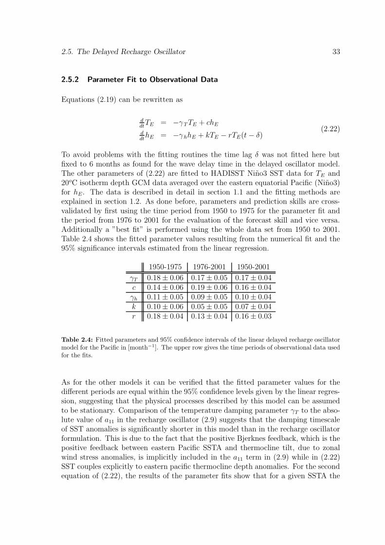
To avoid problems with the fitting routines the time lag δ was not fitted here butfixed to 6 months as found for the wave delay time in the delayed oscillator model.The other parameters of (2.22) are fitted to HADISST Nino3 SST data for TE and20oC isotherm depth GCM data averaged over the eastern equatorial Pacific (Nino3)for hE. The data is described in detail in section 1.1 and the fitting methods areexplained in section 1.2. As done before, parameters and prediction skills are cross-validated by first using the time period from 1950 to 1975 for the parameter fit andthe period from 1976 to 2001 for the evaluation of the forecast skill and vice versa.Additionally a ”best fit” is performed using the whole data set from 1950 to 2001.Table 2.4 shows the fitted parameter values resulting from the numerical fit and the95% significance intervals estimated from the linear regression.
1950-1975 1976-2001 1950-2001
γT 0.18 ± 0.06 0.17 ± 0.05 0.17 ± 0.04c 0.14 ± 0.06 0.19 ± 0.06 0.16 ± 0.04γh 0.11 ± 0.05 0.09 ± 0.05 0.10 ± 0.04k 0.10 ± 0.06 0.05 ± 0.05 0.07 ± 0.04r 0.18 ± 0.04 0.13 ± 0.04 0.16 ± 0.03
Table 2.4: Fitted parameters and 95% confidence intervals of the linear delayed recharge oscillatormodel for the Pacific in [month−1]. The upper row gives the time periods of observational data usedfor the fits.
As for the other models it can be verified that the fitted parameter values for thedifferent periods are equal within the 95% confidence levels given by the linear regres-sion, suggesting that the physical processes described by this model can be assumedto be stationary. Comparison of the temperature damping parameter γT to the abso-lute value of a11 in the recharge oscillator (2.9) suggests that the damping timescaleof SST anomalies is significantly shorter in this model than in the recharge oscillatorformulation. This is due to the fact that the positive Bjerknes feedback, which is thepositive feedback between eastern Pacific SSTA and thermocline tilt, due to zonalwind stress anomalies, is implicitly included in the a11 term in (2.9) while in (2.22)SST couples explicitly to eastern pacific thermocline depth anomalies. For the secondequation of (2.22), the results of the parameter fits show that for a given SSTA the
34 CHAPTER 2. SIMPLE MODELS FOR ENSO
delayed Rossby wave effect (given by −rTE(t−δ)) finally dominates the direct Kelvinwave effect (given by +kTE). This allows for the delayed recharging.
2 4 6 8 10 120
0.5
1SST Correlation
lead month2 4 6 8 10 12
0
0.5
1
SST RMS−error
lead monthst
anda
rd d
evia
tion
2 4 6 8 10 120
0.5
1h Correlation
lead month2 4 6 8 10 12
0
0.5
1
h RMS−error
lead month
stan
dard
dev
iatio
n
1976−2001
1976−2001 Recharge Os.
1950−1975
1950−1975 Recharge Os.
1950−2001
1950−2001 Recharge Os.
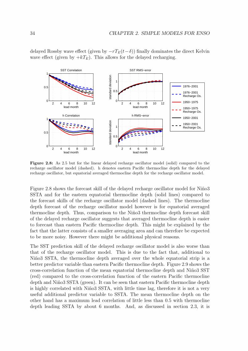
Figure 2.8: As 2.5 but for the linear delayed recharge oscillator model (solid) compared to therecharge oscillator model (dashed). h denotes eastern Pacific thermocline depth for the delayedrecharge oscillator, but equatorial averaged thermocline depth for the recharge oscillator model.
Figure 2.8 shows the forecast skill of the delayed recharge oscillator model for Nino3SSTA and for the eastern equatorial thermocline depth (solid lines) compared tothe forecast skills of the recharge oscillator model (dashed lines). The thermoclinedepth forecast of the recharge oscillator model however is for equatorial averagedthermocline depth. Thus, comparison to the Nino3 thermocline depth forecast skillof the delayed recharge oscillator suggests that averaged thermocline depth is easierto forecast than eastern Pacific thermocline depth. This might be explained by thefact that the latter consists of a smaller averaging area and can therefore be expectedto be more noisy. However there might be additional physical reasons.
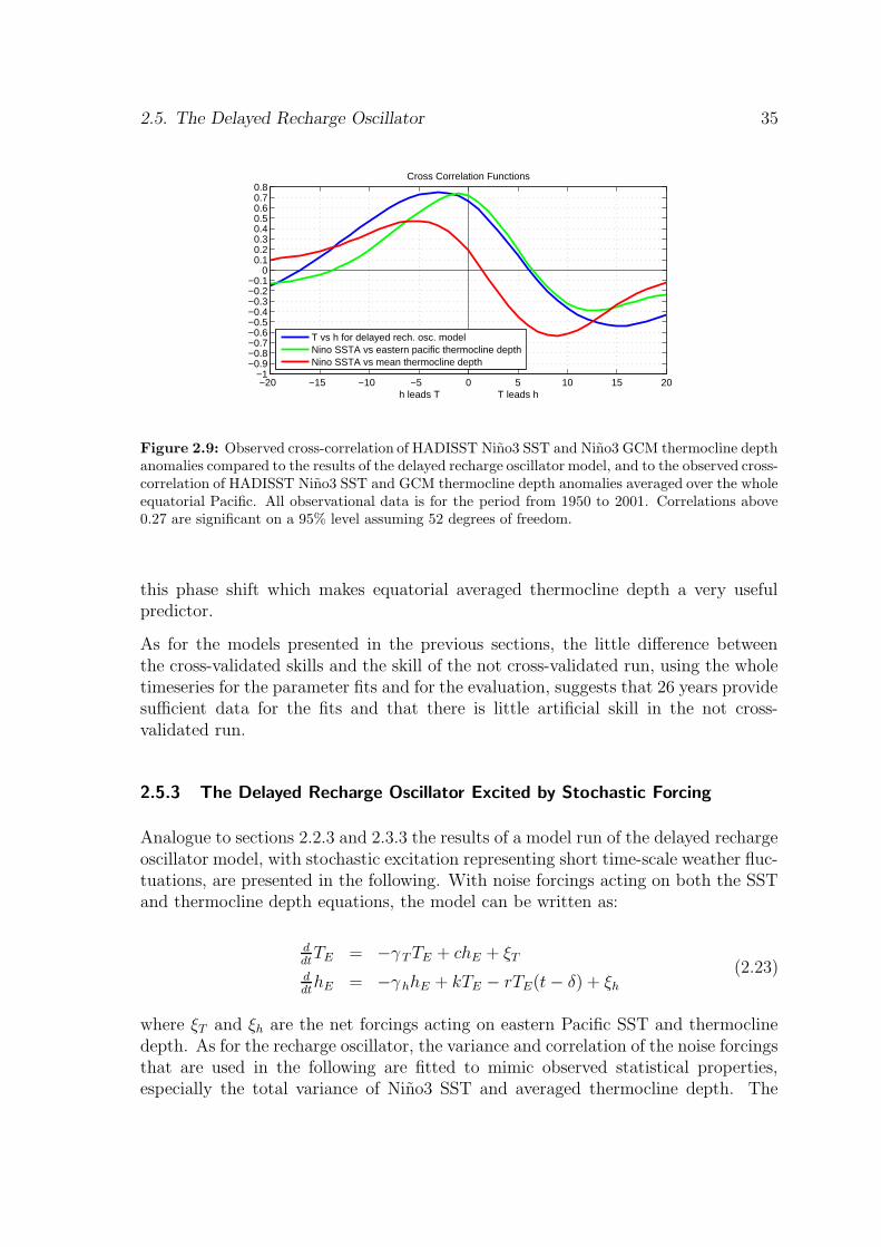
The SST prediction skill of the delayed recharge oscillator model is also worse thanthat of the recharge oscillator model. This is due to the fact that, additional toNino3 SSTA, the thermocline depth averaged over the whole equatorial strip is abetter predictor variable than eastern Pacific thermocline depth. Figure 2.9 shows thecross-correlation function of the mean equatorial thermocline depth and Nino3 SST(red) compared to the cross-correlation function of the eastern Pacific thermoclinedepth and Nino3 SSTA (green). It can be seen that eastern Pacific thermocline depthis highly correlated with Nino3 SSTA, with little time lag, therefore it is not a veryuseful additional predictor variable to SSTA. The mean thermocline depth on theother hand has a maximum lead correlation of little less than 0.5 with thermoclinedepth leading SSTA by about 6 months. And, as discussed in section 2.3, it is
2.5. The Delayed Recharge Oscillator 35
−20 −15 −10 −5 0 5 10 15 20−1
−0.9−0.8−0.7−0.6−0.5−0.4−0.3−0.2−0.1
00.10.20.30.40.50.60.70.8
Cross Correlation Functions
h leads T T leads h
T vs h for delayed rech. osc. modelNino SSTA vs eastern pacific thermocline depthNino SSTA vs mean thermocline depth
Figure 2.9: Observed cross-correlation of HADISST Nino3 SST and Nino3 GCM thermocline depthanomalies compared to the results of the delayed recharge oscillator model, and to the observed cross-correlation of HADISST Nino3 SST and GCM thermocline depth anomalies averaged over the wholeequatorial Pacific. All observational data is for the period from 1950 to 2001. Correlations above0.27 are significant on a 95% level assuming 52 degrees of freedom.
this phase shift which makes equatorial averaged thermocline depth a very usefulpredictor.
As for the models presented in the previous sections, the little difference betweenthe cross-validated skills and the skill of the not cross-validated run, using the wholetimeseries for the parameter fits and for the evaluation, suggests that 26 years providesufficient data for the fits and that there is little artificial skill in the not cross-validated run.
2.5.3 The Delayed Recharge Oscillator Excited by Stochastic Forcing
Analogue to sections 2.2.3 and 2.3.3 the results of a model run of the delayed rechargeoscillator model, with stochastic excitation representing short time-scale weather fluc-tuations, are presented in the following. With noise forcings acting on both the SSTand thermocline depth equations, the model can be written as:
ddt
TE = −γT TE + chE + ξT
ddt
hE = −γhhE + kTE − rTE(t − δ) + ξh
(2.23)
where ξT and ξh are the net forcings acting on eastern Pacific SST and thermoclinedepth. As for the recharge oscillator, the variance and correlation of the noise forcingsthat are used in the following are fitted to mimic observed statistical properties,especially the total variance of Nino3 SST and averaged thermocline depth. The
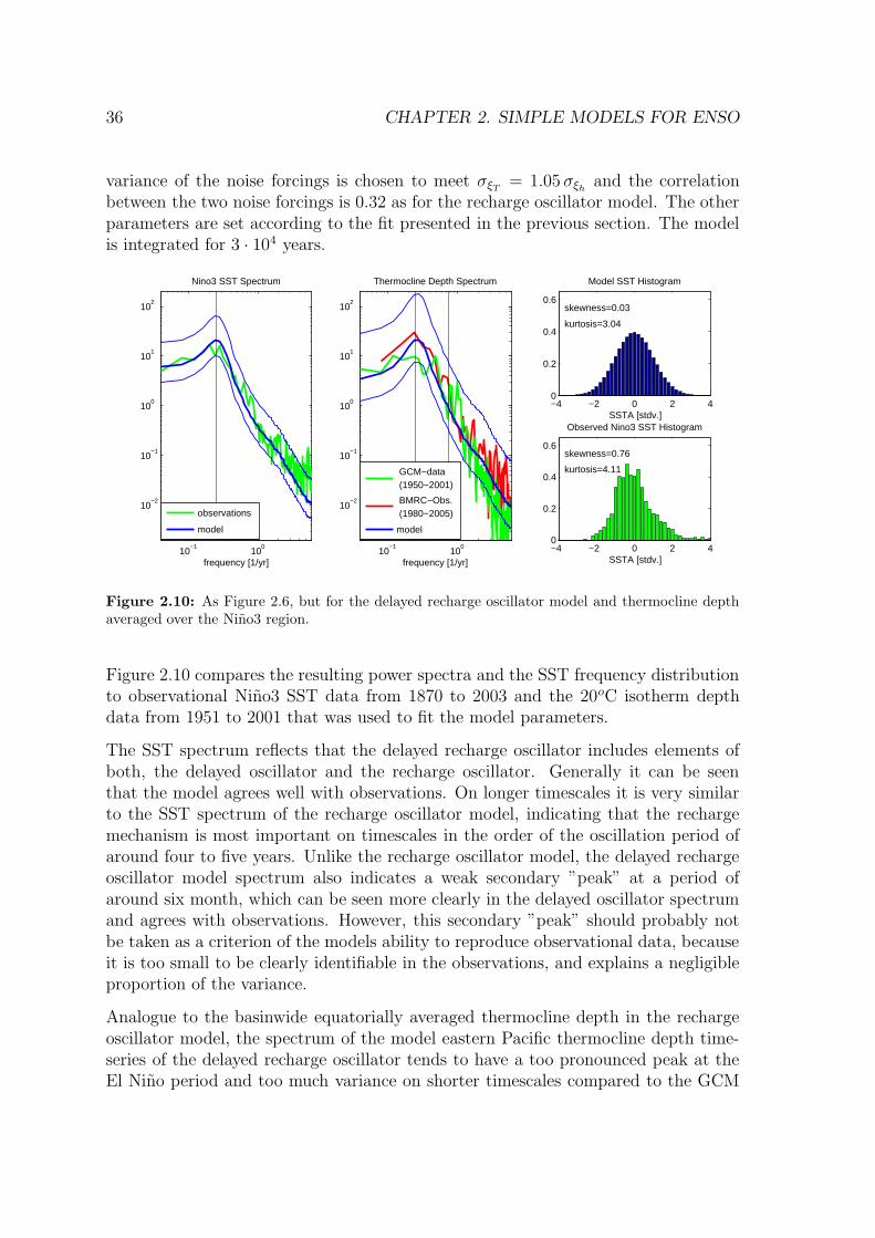
36 CHAPTER 2. SIMPLE MODELS FOR ENSO
variance of the noise forcings is chosen to meet σξT= 1.05 σξh
and the correlationbetween the two noise forcings is 0.32 as for the recharge oscillator model. The otherparameters are set according to the fit presented in the previous section. The modelis integrated for 3 · 104 years.
10−1
100
10−2
10−1
100
101
102
frequency [1/yr]
Nino3 SST Spectrum
observations
model
10−1
100
10−2
10−1
100
101
102
frequency [1/yr]
Thermocline Depth Spectrum
GCM−data (1950−2001)
BMRC−Obs. (1980−2005)
model
−4 −2 0 2 40
0.2
0.4
0.6skewness=0.03
kurtosis=3.04
Model SST Histogram
SSTA [stdv.]
−4 −2 0 2 40
0.2
0.4
0.6skewness=0.76
kurtosis=4.11
Observed Nino3 SST Histogram
SSTA [stdv.]
Figure 2.10: As Figure 2.6, but for the delayed recharge oscillator model and thermocline depthaveraged over the Nino3 region.
Figure 2.10 compares the resulting power spectra and the SST frequency distributionto observational Nino3 SST data from 1870 to 2003 and the 20oC isotherm depthdata from 1951 to 2001 that was used to fit the model parameters.
The SST spectrum reflects that the delayed recharge oscillator includes elements ofboth, the delayed oscillator and the recharge oscillator. Generally it can be seenthat the model agrees well with observations. On longer timescales it is very similarto the SST spectrum of the recharge oscillator model, indicating that the rechargemechanism is most important on timescales in the order of the oscillation period ofaround four to five years. Unlike the recharge oscillator model, the delayed rechargeoscillator model spectrum also indicates a weak secondary ”peak” at a period ofaround six month, which can be seen more clearly in the delayed oscillator spectrumand agrees with observations. However, this secondary ”peak” should probably notbe taken as a criterion of the models ability to reproduce observational data, becauseit is too small to be clearly identifiable in the observations, and explains a negligibleproportion of the variance.
Analogue to the basinwide equatorially averaged thermocline depth in the rechargeoscillator model, the spectrum of the model eastern Pacific thermocline depth time-series of the delayed recharge oscillator tends to have a too pronounced peak at theEl Nino period and too much variance on shorter timescales compared to the GCM
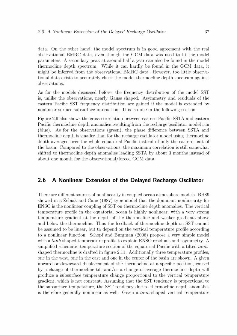
2.6. A Nonlinear Extension of the Delayed Recharge Oscillator 37
data. On the other hand, the model spectrum is in good agreement with the realobservational BMRC data, even though the GCM data was used to fit the modelparameters. A secondary peak at around half a year can also be found in the modelthermocline depth spectrum. While it can hardly be found in the GCM data, itmight be inferred from the observational BMRC data. However, too little observa-tional data exists to accurately check the model thermocline depth spectrum againstobservations.
As for the models discussed before, the frequency distribution of the model SSTis, unlike the observations, nearly Gauss shaped. Asymmetry and residuals of theeastern Pacific SST frequency distribution are gained if the model is extended bynonlinear surface-subsurface interaction. This is done in the following section.
Figure 2.9 also shows the cross-correlation between eastern Pacific SSTA and easternPacific thermocline depth anomalies resulting from the recharge oscillator model run(blue). As for the observations (green), the phase difference between SSTA andthermocline depth is smaller than for the recharge oscillator model using thermoclinedepth averaged over the whole equatorial Pacific instead of only the eastern part ofthe basin. Compared to the observations, the maximum correlation is still somewhatshifted to thermocline depth anomalies leading SSTA by about 3 months instead ofabout one month for the observational/forced GCM data.
2.6 A Nonlinear Extension of the Delayed Recharge Oscillator
There are different sources of nonlinearity in coupled ocean atmosphere models. BH89showed in a Zebiak and Cane (1987) type model that the dominant nonlinearity forENSO is the nonlinear coupling of SST on thermocline depth anomalies. The verticaltemperature profile in the equatorial ocean is highly nonlinear, with a very strongtemperature gradient at the depth of the thermocline and weaker gradients aboveand below the thermocline. Thus the feedback of thermocline depth on SST cannotbe assumed to be linear, but to depend on the vertical temperature profile accordingto a nonlinear function. Schopf and Burgman (2006) propose a very simple modelwith a tanh shaped temperature profile to explain ENSO residuals and asymmetry. Asimplified schematic temperature section of the equatorial Pacific with a tilted tanh-shaped thermocline is drafted in figure 2.11. Additionally three temperature profiles,one in the west, one in the east and one in the center of the basin are shown. A givenupward or downward displacement of the thermocline at a specific position, causedby a change of thermocline tilt and/or a change of average thermocline depth willproduce a subsurface temperature change proportional to the vertical temperaturegradient, which is not constant. Assuming that the SST tendency is proportional tothe subsurface temperature, the SST tendency due to thermocline depth anomaliesis therefore generally nonlinear as well. Given a tanh-shaped vertical temperature
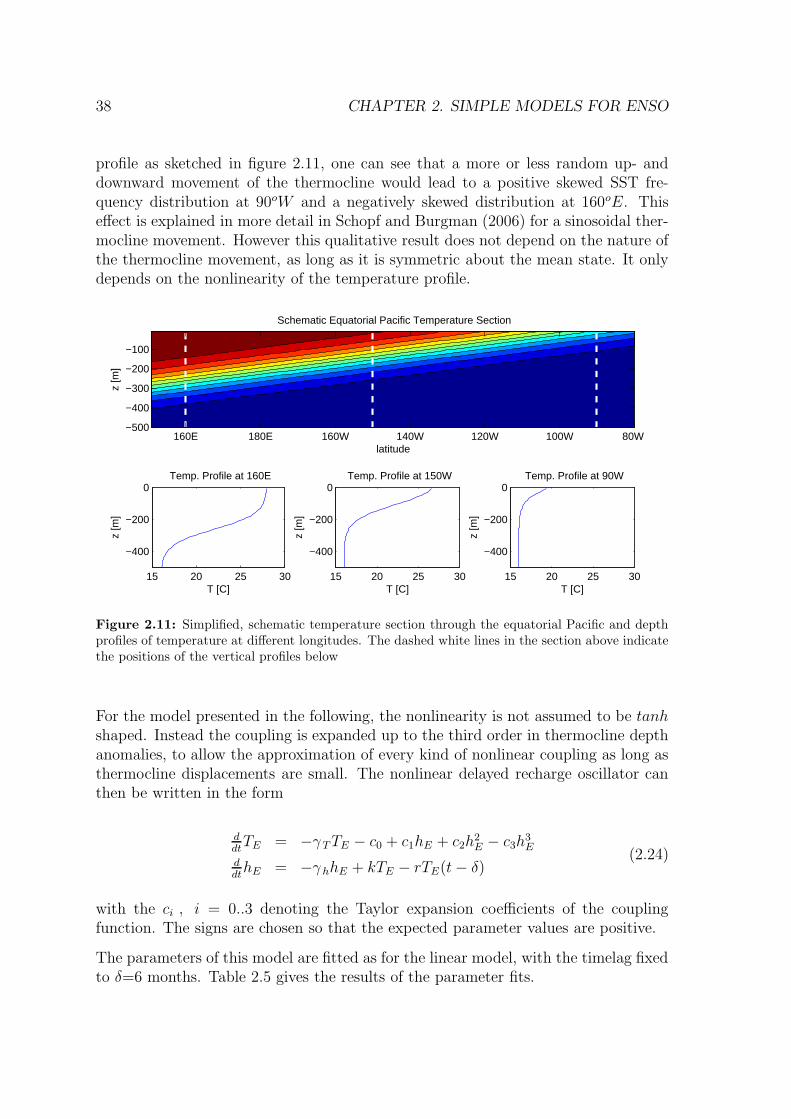
38 CHAPTER 2. SIMPLE MODELS FOR ENSO
profile as sketched in figure 2.11, one can see that a more or less random up- anddownward movement of the thermocline would lead to a positive skewed SST fre-quency distribution at 90oW and a negatively skewed distribution at 160oE. Thiseffect is explained in more detail in Schopf and Burgman (2006) for a sinosoidal ther-mocline movement. However this qualitative result does not depend on the nature ofthe thermocline movement, as long as it is symmetric about the mean state. It onlydepends on the nonlinearity of the temperature profile.
z [m
]
latitude
Schematic Equatorial Pacific Temperature Section
160E 180E 160W 140W 120W 100W 80W −500
−400
−300
−200
−100
15 20 25 30
−400
−200
0
z [m
]
T [C]
Temp. Profile at 160E
15 20 25 30
−400
−200
0
z [m
]
T [C]
Temp. Profile at 150W
15 20 25 30
−400
−200
0
z [m
]
T [C]
Temp. Profile at 90W
Figure 2.11: Simplified, schematic temperature section through the equatorial Pacific and depthprofiles of temperature at different longitudes. The dashed white lines in the section above indicatethe positions of the vertical profiles below
For the model presented in the following, the nonlinearity is not assumed to be tanhshaped. Instead the coupling is expanded up to the third order in thermocline depthanomalies, to allow the approximation of every kind of nonlinear coupling as long asthermocline displacements are small. The nonlinear delayed recharge oscillator canthen be written in the form
ddt
TE = −γT TE − c0 + c1hE + c2h2E − c3h
3E
ddt
hE = −γhhE + kTE − rTE(t − δ)(2.24)
with the ci , i = 0..3 denoting the Taylor expansion coefficients of the couplingfunction. The signs are chosen so that the expected parameter values are positive.
The parameters of this model are fitted as for the linear model, with the timelag fixedto δ=6 months. Table 2.5 gives the results of the parameter fits.
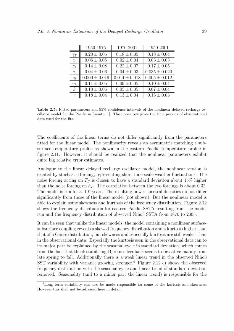
2.6. A Nonlinear Extension of the Delayed Recharge Oscillator 39
1950-1975 1976-2001 1950-2001
γT 0.20 ± 0.06 0.18 ± 0.05 0.18 ± 0.04c0 0.06 ± 0.05 0.02 ± 0.04 0.03 ± 0.03c1 0.14 ± 0.08 0.22 ± 0.07 0.17 ± 0.05c2 0.04 ± 0.06 0.04 ± 0.03 0.035 ± 0.020c3 0.000 ± 0.019 0.014 ± 0.018 0.005 ± 0.012γh 0.11 ± 0.05 0.09 ± 0.05 0.10 ± 0.04k 0.10 ± 0.06 0.05 ± 0.05 0.07 ± 0.04r 0.18 ± 0.04 0.13 ± 0.04 0.15 ± 0.03
Table 2.5: Fitted parameters and 95% confidence intervals of the nonlinear delayed recharge os-cillator model for the Pacific in [month−1]. The upper row gives the time periods of observationaldata used for the fits.
The coefficients of the linear terms do not differ significantly from the parametersfitted for the linear model. The nonlinearity reveals an asymmetrie matching a sub-surface temperature profile as shown in the eastern Pacific temperature profile infigure 2.11. However, it should be realized that the nonlinear parameters exhibitquite big relative error estimates.
Analogue to the linear delayed recharge oscillator model, the nonlinear version isexcited by stochastic forcing, representing short time-scale weather fluctuations. Thenoise forcing acting on TE is chosen to have a standard deviation about 15% higherthan the noise forcing on hE. The correlation between the two forcings is about 0.32.The model is run for 3 ·104 years. The resulting power spectral densities do not differsignificantly from those of the linear model (not shown). But the nonlinear model isable to explain some skewness and kurtosis of the frequency distribution. Figure 2.12shows the frequency distribution for eastern Pacific SSTA resulting from the modelrun and the frequency distribution of observed Nino3 SSTA from 1870 to 2003.
It can be seen that unlike the linear models, the model containing a nonlinear surface-subsurface coupling reveals a skewed frequency distribution and a kurtosis higher thanthat of a Gauss distribution, but skewness and especially kurtosis are still weaker thanin the observational data. Especially the kurtosis seen in the observational data can toits major part be explained by the seasonal cycle in standard deviation, which comesfrom the fact that the destabilising Bjerknes feedback seems to be active mainly fromlate spring to fall. Additionally there is a weak linear trend in the observed Nino3SST variability with variance growing stronger.9 Figure 2.12 c) shows the observedfrequency distribution with the seasonal cycle and linear trend of standard deviationremoved. Seasonality (and to a minor part the linear trend) is responsible for the
9Long term variability can also be made responsible for some of the kurtosis and skewness.However this shall not be adressed here in detail.
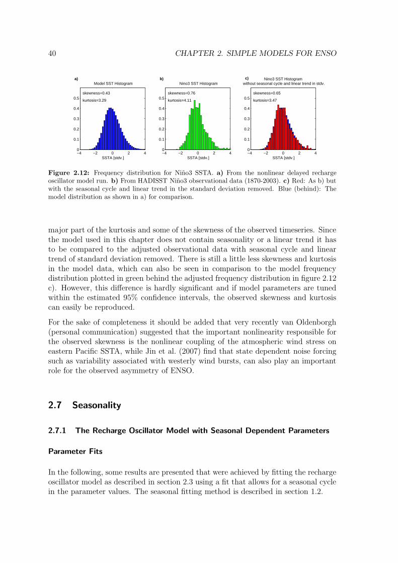
40 CHAPTER 2. SIMPLE MODELS FOR ENSO
−4 −2 0 2 40
0.1
0.2
0.3
0.4
0.5skewness=0.43
kurtosis=3.29
Model SST Histogram
SSTA [stdv.]
a)
−4 −2 0 2 40
0.1
0.2
0.3
0.4
0.5skewness=0.76
kurtosis=4.11
Nino3 SST Histogram
SSTA [stdv.]
b)
−4 −2 0 2 40
0.1
0.2
0.3
0.4
0.5skewness=0.65
kurtosis=3.47
Nino3 SST Histogram without seasonal cycle and linear trend in stdv.
SSTA [stdv.]
c)
Figure 2.12: Frequency distribution for Nino3 SSTA. a) From the nonlinear delayed rechargeoscillator model run. b) From HADISST Nino3 observational data (1870-2003). c) Red: As b) butwith the seasonal cycle and linear trend in the standard deviation removed. Blue (behind): Themodel distribution as shown in a) for comparison.
major part of the kurtosis and some of the skewness of the observed timeseries. Sincethe model used in this chapter does not contain seasonality or a linear trend it hasto be compared to the adjusted observational data with seasonal cycle and lineartrend of standard deviation removed. There is still a little less skewness and kurtosisin the model data, which can also be seen in comparison to the model frequencydistribution plotted in green behind the adjusted frequency distribution in figure 2.12c). However, this difference is hardly significant and if model parameters are tunedwithin the estimated 95% confidence intervals, the observed skewness and kurtosiscan easily be reproduced.
For the sake of completeness it should be added that very recently van Oldenborgh(personal communication) suggested that the important nonlinearity responsible forthe observed skewness is the nonlinear coupling of the atmospheric wind stress oneastern Pacific SSTA, while Jin et al. (2007) find that state dependent noise forcingsuch as variability associated with westerly wind bursts, can also play an importantrole for the observed asymmetry of ENSO.
2.7 Seasonality
2.7.1 The Recharge Oscillator Model with Seasonal Dependent Parameters
Parameter Fits
In the following, some results are presented that were achieved by fitting the rechargeoscillator model as described in section 2.3 using a fit that allows for a seasonal cyclein the parameter values. The seasonal fitting method is described in section 1.2.
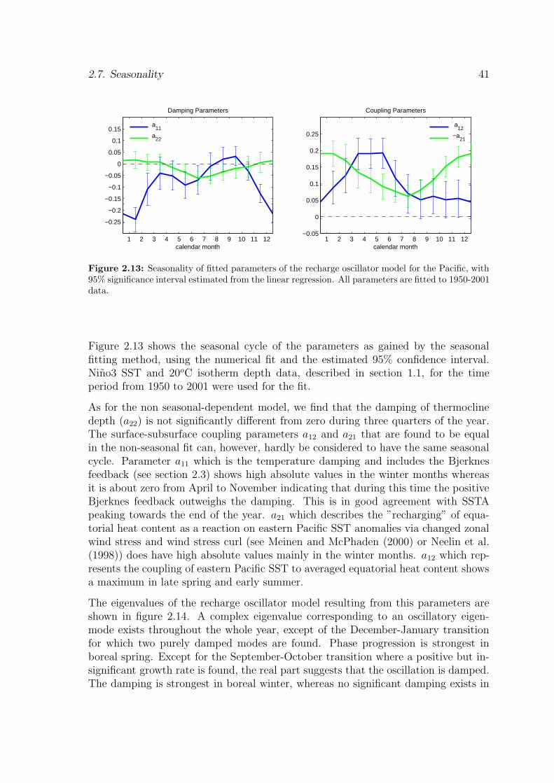
2.7. Seasonality 41
1 2 3 4 5 6 7 8 9 10 11 12
−0.25
−0.2
−0.15
−0.1
−0.05
0
0.05
0.1
0.15
Damping Parameters
calendar month
a
11
a22
1 2 3 4 5 6 7 8 9 10 11 12−0.05
0
0.05
0.1
0.15
0.2
0.25
Coupling Parameters
calendar month
a
12
−a21
Figure 2.13: Seasonality of fitted parameters of the recharge oscillator model for the Pacific, with95% significance interval estimated from the linear regression. All parameters are fitted to 1950-2001data.
Figure 2.13 shows the seasonal cycle of the parameters as gained by the seasonalfitting method, using the numerical fit and the estimated 95% confidence interval.Nino3 SST and 20oC isotherm depth data, described in section 1.1, for the timeperiod from 1950 to 2001 were used for the fit.
As for the non seasonal-dependent model, we find that the damping of thermoclinedepth (a22) is not significantly different from zero during three quarters of the year.The surface-subsurface coupling parameters a12 and a21 that are found to be equalin the non-seasonal fit can, however, hardly be considered to have the same seasonalcycle. Parameter a11 which is the temperature damping and includes the Bjerknesfeedback (see section 2.3) shows high absolute values in the winter months whereasit is about zero from April to November indicating that during this time the positiveBjerknes feedback outweighs the damping. This is in good agreement with SSTApeaking towards the end of the year. a21 which describes the ”recharging” of equa-torial heat content as a reaction on eastern Pacific SST anomalies via changed zonalwind stress and wind stress curl (see Meinen and McPhaden (2000) or Neelin et al.(1998)) does have high absolute values mainly in the winter months. a12 which rep-resents the coupling of eastern Pacific SST to averaged equatorial heat content showsa maximum in late spring and early summer.
The eigenvalues of the recharge oscillator model resulting from this parameters areshown in figure 2.14. A complex eigenvalue corresponding to an oscillatory eigen-mode exists throughout the whole year, except of the December-January transitionfor which two purely damped modes are found. Phase progression is strongest inboreal spring. Except for the September-October transition where a positive but in-significant growth rate is found, the real part suggests that the oscillation is damped.The damping is strongest in boreal winter, whereas no significant damping exists in
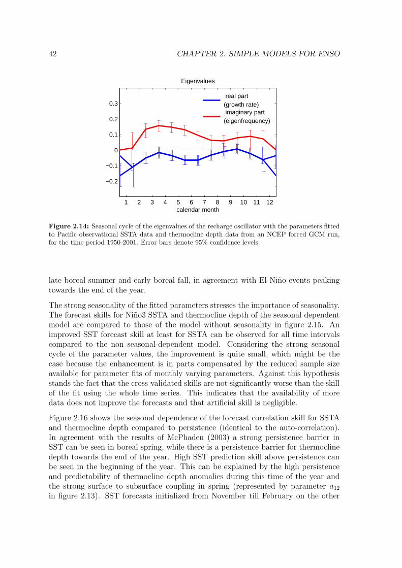
42 CHAPTER 2. SIMPLE MODELS FOR ENSO
1 2 3 4 5 6 7 8 9 10 11 12
−0.2
−0.1
0
0.1
0.2
0.3
Eigenvalues
calendar month
real part (growth rate) imaginary part (eigenfrequency)
Figure 2.14: Seasonal cycle of the eigenvalues of the recharge oscillator with the parameters fittedto Pacific observational SSTA data and thermocline depth data from an NCEP forced GCM run,for the time period 1950-2001. Error bars denote 95% confidence levels.
late boreal summer and early boreal fall, in agreement with El Nino events peakingtowards the end of the year.
The strong seasonality of the fitted parameters stresses the importance of seasonality.The forecast skills for Nino3 SSTA and thermocline depth of the seasonal dependentmodel are compared to those of the model without seasonality in figure 2.15. Animproved SST forecast skill at least for SSTA can be observed for all time intervalscompared to the non seasonal-dependent model. Considering the strong seasonalcycle of the parameter values, the improvement is quite small, which might be thecase because the enhancement is in parts compensated by the reduced sample sizeavailable for parameter fits of monthly varying parameters. Against this hypothesisstands the fact that the cross-validated skills are not significantly worse than the skillof the fit using the whole time series. This indicates that the availability of moredata does not improve the forecasts and that artificial skill is negligible.
Figure 2.16 shows the seasonal dependence of the forecast correlation skill for SSTAand thermocline depth compared to persistence (identical to the auto-correlation).In agreement with the results of McPhaden (2003) a strong persistence barrier inSST can be seen in boreal spring, while there is a persistence barrier for thermoclinedepth towards the end of the year. High SST prediction skill above persistence canbe seen in the beginning of the year. This can be explained by the high persistenceand predictability of thermocline depth anomalies during this time of the year andthe strong surface to subsurface coupling in spring (represented by parameter a12
in figure 2.13). SST forecasts initialized from November till February on the other
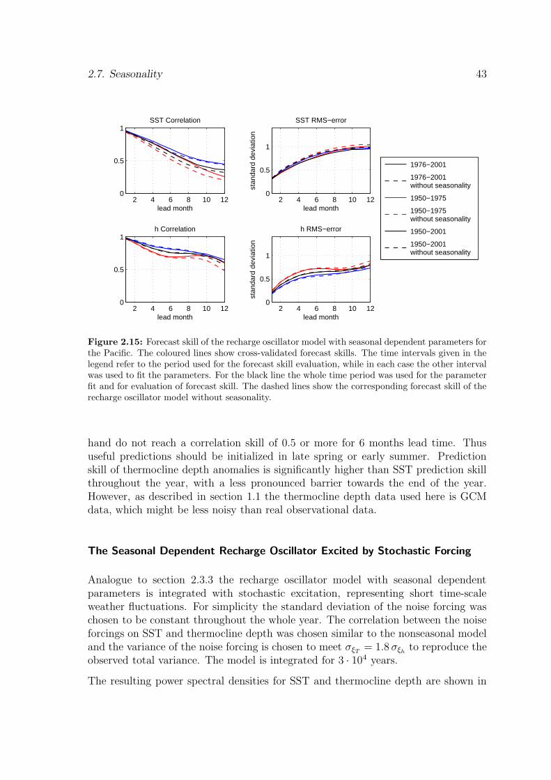
2.7. Seasonality 43
2 4 6 8 10 120
0.5
1SST Correlation
lead month2 4 6 8 10 12
0
0.5
1
SST RMS−error
lead month
stan
dard
dev
iatio
n
2 4 6 8 10 120
0.5
1h Correlation
lead month2 4 6 8 10 12
0
0.5
1
h RMS−error
lead month
stan
dard
dev
iatio
n
1976−2001
1976−2001 without seasonality
1950−1975
1950−1975 without seasonality
1950−2001
1950−2001 without seasonality
Figure 2.15: Forecast skill of the recharge oscillator model with seasonal dependent parameters forthe Pacific. The coloured lines show cross-validated forecast skills. The time intervals given in thelegend refer to the period used for the forecast skill evaluation, while in each case the other intervalwas used to fit the parameters. For the black line the whole time period was used for the parameterfit and for evaluation of forecast skill. The dashed lines show the corresponding forecast skill of therecharge oscillator model without seasonality.
hand do not reach a correlation skill of 0.5 or more for 6 months lead time. Thususeful predictions should be initialized in late spring or early summer. Predictionskill of thermocline depth anomalies is significantly higher than SST prediction skillthroughout the year, with a less pronounced barrier towards the end of the year.However, as described in section 1.1 the thermocline depth data used here is GCMdata, which might be less noisy than real observational data.
The Seasonal Dependent Recharge Oscillator Excited by Stochastic Forcing
Analogue to section 2.3.3 the recharge oscillator model with seasonal dependentparameters is integrated with stochastic excitation, representing short time-scaleweather fluctuations. For simplicity the standard deviation of the noise forcing waschosen to be constant throughout the whole year. The correlation between the noiseforcings on SST and thermocline depth was chosen similar to the nonseasonal modeland the variance of the noise forcing is chosen to meet σξT
= 1.8 σξhto reproduce the
observed total variance. The model is integrated for 3 · 104 years.
The resulting power spectral densities for SST and thermocline depth are shown in
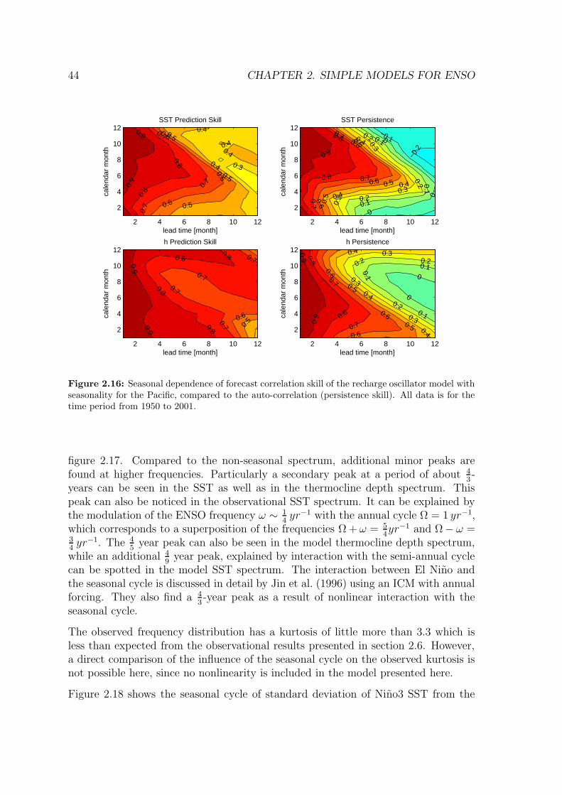
44 CHAPTER 2. SIMPLE MODELS FOR ENSO
0.3
0.4
0.4
0.5
0.5
0.5
0.6
0.6
0.6
0.7
0.7
0.7
0.8
0.8
0.90.
9
0.40.4
lead time [month]
cale
ndar
mon
th
SST Prediction Skill
2 4 6 8 10 12
2
4
6
8
10
12
−0.2
−0.10
0
0
0.10.1
0.1
0.20.2
0.20.3
0.3
0.3
0.4
0.4
0.4
0.5
0.5
0.5
0.6
0.6
0.6
0.7
0.7
0.7
0.8
0.8
0.9
lead time [month]
cale
ndar
mon
th
SST Persistence
2 4 6 8 10 12
2
4
6
8
10
12
0.50.6
0.7
0.70.7
0.7
0.80.8
0.8
0.8
0.9
0.9
lead time [month]
cale
ndar
mon
th
h Prediction Skill
2 4 6 8 10 12
2
4
6
8
10
12
0
0
0.10.1
0.1
0.20.2
0.2
0.3
0.3
0.3
0.4
0.4
0.4
0.5
0.5
0.6
0.6
0.6
0.7
0.7
0.8
0.8
0.9
0.9
lead time [month]
cale
ndar
mon
th
h Persistence
2 4 6 8 10 12
2
4
6
8
10
12
Figure 2.16: Seasonal dependence of forecast correlation skill of the recharge oscillator model withseasonality for the Pacific, compared to the auto-correlation (persistence skill). All data is for thetime period from 1950 to 2001.
figure 2.17. Compared to the non-seasonal spectrum, additional minor peaks arefound at higher frequencies. Particularly a secondary peak at a period of about 4
3-
years can be seen in the SST as well as in the thermocline depth spectrum. Thispeak can also be noticed in the observational SST spectrum. It can be explained bythe modulation of the ENSO frequency ω ∼ 1
4yr−1 with the annual cycle Ω = 1 yr−1,
which corresponds to a superposition of the frequencies Ω + ω = 54yr−1 and Ω− ω =
34yr−1. The 4
5year peak can also be seen in the model thermocline depth spectrum,
while an additional 49
year peak, explained by interaction with the semi-annual cyclecan be spotted in the model SST spectrum. The interaction between El Nino andthe seasonal cycle is discussed in detail by Jin et al. (1996) using an ICM with annualforcing. They also find a 4
3-year peak as a result of nonlinear interaction with the
seasonal cycle.
The observed frequency distribution has a kurtosis of little more than 3.3 which isless than expected from the observational results presented in section 2.6. However,a direct comparison of the influence of the seasonal cycle on the observed kurtosis isnot possible here, since no nonlinearity is included in the model presented here.
Figure 2.18 shows the seasonal cycle of standard deviation of Nino3 SST from the
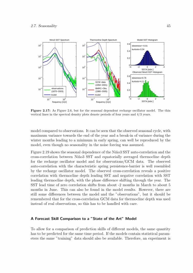
2.7. Seasonality 45
10−1
100
10−2
10−1
100
101
102
frequency [1/yr]
Nino3 SST Spectrum
observations (1870−2003)
model
10−1
100
10−2
10−1
100
101
102
frequency [1/yr]
Thermocline Depth Spectrum
GCM−data (1950−2001)
BMRC−Obs. (1980−2005)
model
−4 −2 0 2 40
0.2
0.4
0.6skewness=−0.01
kurtosis=3.34
Model SST Histogram
SSTA [stdv.]
−4 −2 0 2 40
0.2
0.4
0.6skewness=0.76
kurtosis=4.11
Observed Nino3 SST Histogram
SSTA [stdv.]
Figure 2.17: As Figure 2.6, but for the seasonal dependent recharge oscillator model. The thinvertical lines in the spectral density plots denote periods of four years and 4/3 years.
model compared to observations. It can be seen that the observed seasonal cycle, withmaximum variance towards the end of the year and a break-in of variance during thewinter months leading to a minimum in early spring, can well be reproduced by themodel, even though no seasonality in the noise forcing was assumed.
Figure 2.19 shows the seasonal dependence of the Nino3 SST auto-correlation and thecross-correlation between Nino3 SST and equatorially averaged thermocline depthfor the recharge oscillator model and for observations/GCM data. The observedauto-correlation with the characteristic spring persistence-barrier is well resembledby the recharge oscillator model. The observed cross-correlation reveals a positivecorrelation with thermocline depth leading SST and negative correlation with SSTleading thermocline depth, with the phase difference shifting through the year. TheSST lead time of zero correlation shifts from about -2 months in March to about 5months in June. This can also be found in the model results. However, there arestill some differences between the model and the ”observations”, but it should beremembered that for the cross-correlation GCM data for thermocline depth was usedinstead of real observations, so this has to be handled with care.
A Forecast Skill Comparison to a ”State of the Art” Model
To allow for a comparison of prediction skills of different models, the same quantityhas to be predicted for the same time period. If the models contain statistical param-eters the same ”training” data should also be available. Therefore, an experiment is
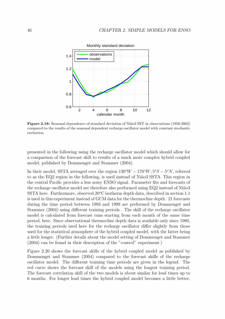
46 CHAPTER 2. SIMPLE MODELS FOR ENSO
2 4 6 8 10 120.6
0.8
1
1.2
1.4
Monthly standard deviation
calendar month
observationsmodel
Figure 2.18: Seasonal dependence of standard deviation of Nino3 SST in observations (1950-2002)compared to the results of the seasonal dependent recharge oscillator model with constant stochasticexcitation.
presented in the following using the recharge oscillator model which should allow fora comparison of the forecast skill to results of a much more complex hybrid coupledmodel, published by Dommenget and Stammer (2004).
In their model, SSTA averaged over the region 130oW − 170oW ; 5oS − 5oN , referredto as the EQ2 region in the following, is used instead of Nino3 SSTA. This region inthe central Pacific provides a less noisy ENSO signal. Parameter fits and forecasts ofthe recharge oscillator model are therefore also performed using EQ2 instead of Nino3SSTA here. Furthermore, observed 20oC isotherm depth data, described in section 1.1is used in this experiment instead of GCM data for the thermocline depth. 21 forecastsduring the time period between 1993 and 1999 are performed by Dommenget andStammer (2004) using different training periods . The skill of the recharge oscillatormodel is calculated from forecast runs starting from each month of the same timeperiod, here. Since observational thermocline depth data is available only since 1980,the training periods used here for the recharge oscillator differ slightly from thoseused for the statistical atmosphere of the hybrid coupled model, with the latter beinga little longer. (Further details about the model setting of Dommenget and Stammer(2004) can be found in their description of the ”control” experiment.)
Figure 2.20 shows the forecast skills of the hybrid coupled model as published byDommenget and Stammer (2004) compared to the forecast skills of the rechargeoscillator model. The different training time periods are given in the legend. Thered curve shows the forecast skill of the models using the longest training period.The forecast correlation skill of the two models is about similar for lead times up to6 months. For longer lead times the hybrid coupled model becomes a little better.
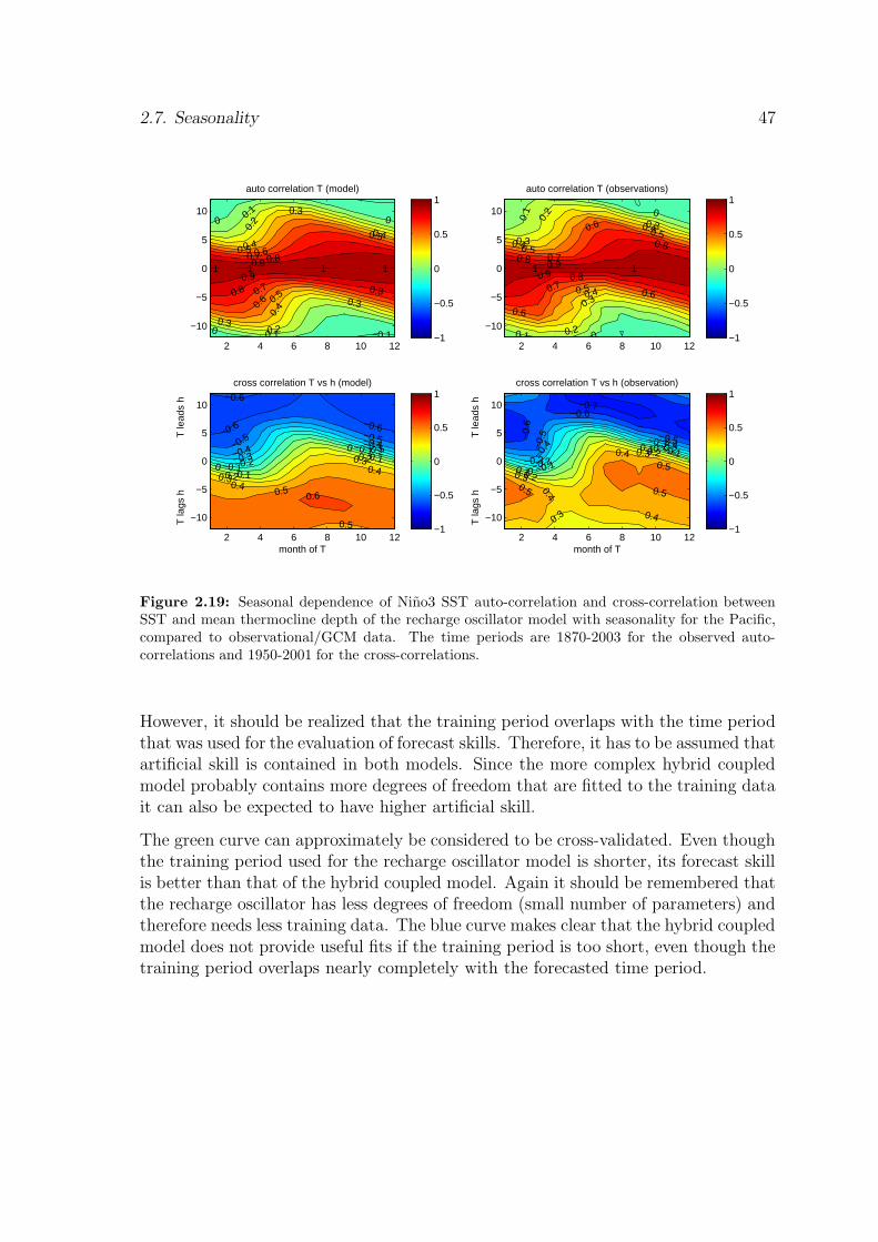
2.7. Seasonality 47
−0.1
0 0
0
0.1
0.1
0.2
0.2
0.3
0.3
0.3
0.40.4
0.4
0.5
0.5
0.5
0.6
0.6
0.7
0.7
0.8
0.80.8
0.9
0.91 11 1
auto correlation T (model)
2 4 6 8 10 12
−10
−5
0
5
10
−1
−0.5
0
0.5
10
0
0.1
0.1
0.2
0.2
0.3
0.3
0.3
0.4
0.4
0.4
0.5
0.5
0.5
0.6
0.6
0.6
0.7
0.7
0.8
0.8
0.80.9
0.91 1
auto correlation T (observations)
2 4 6 8 10 12
−10
−5
0
5
10
−1
−0.5
0
0.5
1
−0.6 −0.6
−0.5 −0.5
−0.4−0.4
−0.3−0.3
−0.2
−0.2
−0.1
−0.1
0
0
0.1
0.1
0.2
0.2
0.3
0.3
0.4
0.4
0.5
0.5
0.6
−0.6
cross correlation T vs h (model)
month of T
T la
gs h
T le
ads
h
2 4 6 8 10 12
−10
−5
0
5
10
−1
−0.5
0
0.5
1−0.7
−0.6
−0.
6−0
.5 −0.5
−0.4
−0.4
−0.3
−0.3
−0.2
−0.2
−0.1
−0.1
0
0
0.1
0.1
0.2
0.2
0.3
0.3
0.3 0.4
0.4
0.5
0.5
0.4
0.5
cross correlation T vs h (observation)
month of T
T la
gs h
T le
ads
h
2 4 6 8 10 12
−10
−5
0
5
10
−1
−0.5
0
0.5
1
Figure 2.19: Seasonal dependence of Nino3 SST auto-correlation and cross-correlation betweenSST and mean thermocline depth of the recharge oscillator model with seasonality for the Pacific,compared to observational/GCM data. The time periods are 1870-2003 for the observed auto-correlations and 1950-2001 for the cross-correlations.
However, it should be realized that the training period overlaps with the time periodthat was used for the evaluation of forecast skills. Therefore, it has to be assumed thatartificial skill is contained in both models. Since the more complex hybrid coupledmodel probably contains more degrees of freedom that are fitted to the training datait can also be expected to have higher artificial skill.
The green curve can approximately be considered to be cross-validated. Even thoughthe training period used for the recharge oscillator model is shorter, its forecast skillis better than that of the hybrid coupled model. Again it should be remembered thatthe recharge oscillator has less degrees of freedom (small number of parameters) andtherefore needs less training data. The blue curve makes clear that the hybrid coupledmodel does not provide useful fits if the training period is too short, even though thetraining period overlaps nearly completely with the forecasted time period.
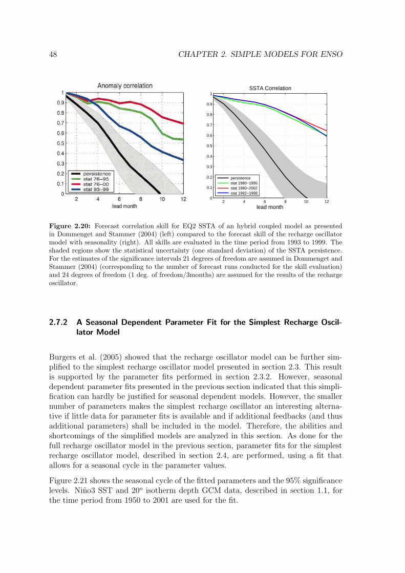
48 CHAPTER 2. SIMPLE MODELS FOR ENSO
2 4 6 8 10 120
0.1
0.2
0.3
0.4
0.5
0.6
0.7
0.8
0.9
1SSTA Correlation
lead month
persistence stat 1980−1995 stat 1980−2002 stat 1992−1998
Figure 2.20: Forecast correlation skill for EQ2 SSTA of an hybrid coupled model as presentedin Dommenget and Stammer (2004) (left) compared to the forecast skill of the recharge oscillatormodel with seasonality (right). All skills are evaluated in the time period from 1993 to 1999. Theshaded regions show the statistical uncertainty (one standard deviation) of the SSTA persistence.For the estimates of the significance intervals 21 degrees of freedom are assumed in Dommenget andStammer (2004) (corresponding to the number of forecast runs conducted for the skill evaluation)and 24 degrees of freedom (1 deg. of freedom/3months) are assumed for the results of the rechargeoscillator.
2.7.2 A Seasonal Dependent Parameter Fit for the Simplest Recharge Oscil-lator Model
Burgers et al. (2005) showed that the recharge oscillator model can be further sim-plified to the simplest recharge oscillator model presented in section 2.3. This resultis supported by the parameter fits performed in section 2.3.2. However, seasonaldependent parameter fits presented in the previous section indicated that this simpli-fication can hardly be justified for seasonal dependent models. However, the smallernumber of parameters makes the simplest recharge oscillator an interesting alterna-tive if little data for parameter fits is available and if additional feedbacks (and thusadditional parameters) shall be included in the model. Therefore, the abilities andshortcomings of the simplified models are analyzed in this section. As done for thefull recharge oscillator model in the previous section, parameter fits for the simplestrecharge oscillator model, described in section 2.4, are performed, using a fit thatallows for a seasonal cycle in the parameter values.
Figure 2.21 shows the seasonal cycle of the fitted parameters and the 95% significancelevels. Nino3 SST and 20o isotherm depth GCM data, described in section 1.1, forthe time period from 1950 to 2001 are used for the fit.
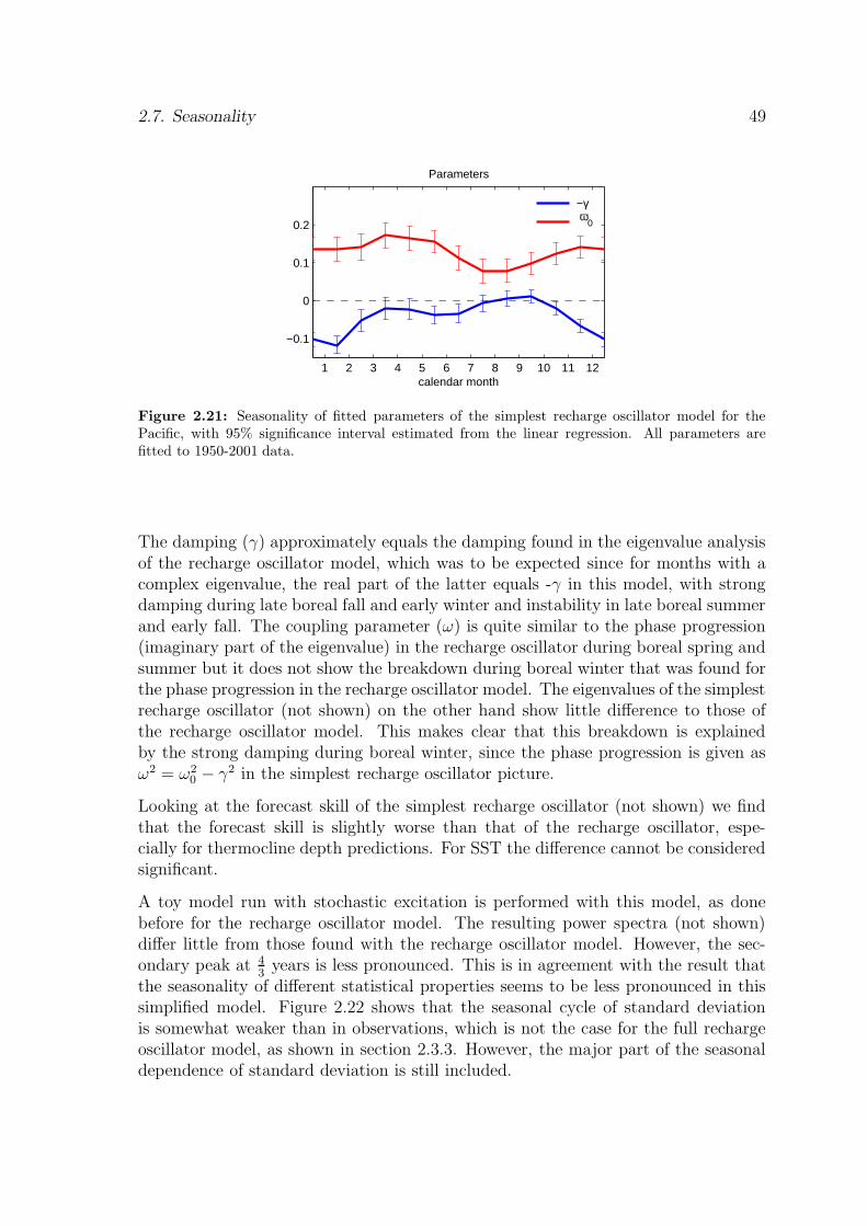
2.7. Seasonality 49
1 2 3 4 5 6 7 8 9 10 11 12
−0.1
0
0.1
0.2
Parameters
calendar month
−γ ω
0
Figure 2.21: Seasonality of fitted parameters of the simplest recharge oscillator model for thePacific, with 95% significance interval estimated from the linear regression. All parameters arefitted to 1950-2001 data.
The damping (γ) approximately equals the damping found in the eigenvalue analysisof the recharge oscillator model, which was to be expected since for months with acomplex eigenvalue, the real part of the latter equals -γ in this model, with strongdamping during late boreal fall and early winter and instability in late boreal summerand early fall. The coupling parameter (ω) is quite similar to the phase progression(imaginary part of the eigenvalue) in the recharge oscillator during boreal spring andsummer but it does not show the breakdown during boreal winter that was found forthe phase progression in the recharge oscillator model. The eigenvalues of the simplestrecharge oscillator (not shown) on the other hand show little difference to those ofthe recharge oscillator model. This makes clear that this breakdown is explainedby the strong damping during boreal winter, since the phase progression is given asω2 = ω2
0 − γ2 in the simplest recharge oscillator picture.
Looking at the forecast skill of the simplest recharge oscillator (not shown) we findthat the forecast skill is slightly worse than that of the recharge oscillator, espe-cially for thermocline depth predictions. For SST the difference cannot be consideredsignificant.
A toy model run with stochastic excitation is performed with this model, as donebefore for the recharge oscillator model. The resulting power spectra (not shown)differ little from those found with the recharge oscillator model. However, the sec-ondary peak at 4
3years is less pronounced. This is in agreement with the result that
the seasonality of different statistical properties seems to be less pronounced in thissimplified model. Figure 2.22 shows that the seasonal cycle of standard deviationis somewhat weaker than in observations, which is not the case for the full rechargeoscillator model, as shown in section 2.3.3. However, the major part of the seasonaldependence of standard deviation is still included.
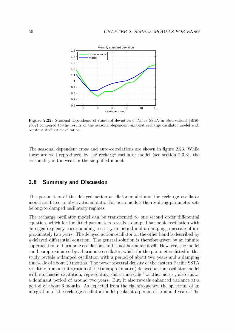
50 CHAPTER 2. SIMPLE MODELS FOR ENSO
2 4 6 8 10 120.6
0.7
0.8
0.9
1
1.1
1.2
1.3
1.4
1.5Monthly standard deviation
calendar month
observationsmodel
Figure 2.22: Seasonal dependence of standard deviation of Nino3 SSTA in observations (1950-2002) compared to the results of the seasonal dependent simplest recharge oscillator model withconstant stochastic excitation.
The seasonal dependent cross and auto-correlations are shown in figure 2.23. Whilethese are well reproduced by the recharge oscillator model (see section 2.3.3), theseasonality is too weak in the simplified model.
2.8 Summary and Discussion
The parameters of the delayed action oscillator model and the recharge oscillatormodel are fitted to observational data. For both models the resulting parameter setsbelong to damped oscillatory regimes.
The recharge oscillator model can be transformed to one second order differentialequation, which for the fitted parameters reveals a damped harmonic oscillation withan eigenfrequency corresponding to a 4-year period and a damping timescale of ap-proximately two years. The delayed action oscillator on the other hand is described bya delayed differential equation. The general solution is therefore given by an infinitesuperposition of harmonic oscillations and is not harmonic itself. However, the modelcan be approximated by a harmonic oscillator, which for the parameters fitted in thisstudy reveals a damped oscillation with a period of about two years and a dampingtimescale of about 20 months. The power spectral density of the eastern Pacific SSTAresulting from an integration of the (unapproximated) delayed action oscillator modelwith stochastic excitation, representing short-timescale ”weather-noise”, also showsa dominant period of around two years. But, it also reveals enhanced variance at aperiod of about 6 months. As expected from the eigenfrequency, the spectrum of anintegration of the recharge oscillator model peaks at a period of around 4 years. The
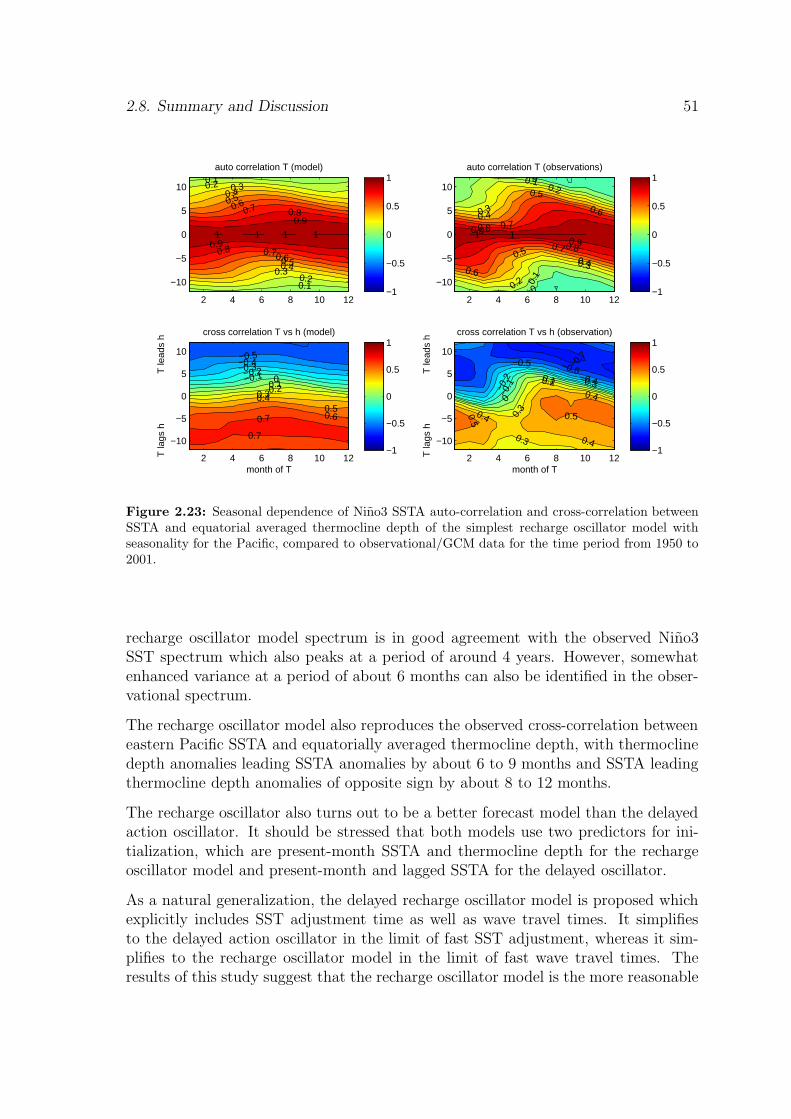
2.8. Summary and Discussion 51
0.1
0.1
0.2
0.2
0.3
0.3
0.4
0.4
0.5
0.5
0.6
0.6
0.7
0.7
0.8
0.8
0.9
0.911 1 1
auto correlation T (model)
2 4 6 8 10 12
−10
−5
0
5
10
−1
−0.5
0
0.5
1 0
0
0.1
0.1
0.2
0.2
0.3
0.3
0.4
0.4
0.5
0.5
0.6
0.6
0.7
0.7
0.8
0.8
0.90.9
11
auto correlation T (observations)
2 4 6 8 10 12
−10
−5
0
5
10
−1
−0.5
0
0.5
1
−0.5−0.4−0.3
−0.2−0.1 0
0.10.20.30.4
0.50.60.7
0.7
cross correlation T vs h (model)
month of T
T la
gs h
T le
ads
h
2 4 6 8 10 12
−10
−5
0
5
10
−1
−0.5
0
0.5
1
−0.7
−0.6−0.5
−0.4−0.3
−0.2
−0.1
0
0.10.2
0.3
0.3 0.4
0.4
0.50.40.5
cross correlation T vs h (observation)
month of T
T la
gs h
T le
ads
h
2 4 6 8 10 12
−10
−5
0
5
10
−1
−0.5
0
0.5
1
Figure 2.23: Seasonal dependence of Nino3 SSTA auto-correlation and cross-correlation betweenSSTA and equatorial averaged thermocline depth of the simplest recharge oscillator model withseasonality for the Pacific, compared to observational/GCM data for the time period from 1950 to2001.
recharge oscillator model spectrum is in good agreement with the observed Nino3SST spectrum which also peaks at a period of around 4 years. However, somewhatenhanced variance at a period of about 6 months can also be identified in the obser-vational spectrum.
The recharge oscillator model also reproduces the observed cross-correlation betweeneastern Pacific SSTA and equatorially averaged thermocline depth, with thermoclinedepth anomalies leading SSTA anomalies by about 6 to 9 months and SSTA leadingthermocline depth anomalies of opposite sign by about 8 to 12 months.
The recharge oscillator also turns out to be a better forecast model than the delayedaction oscillator. It should be stressed that both models use two predictors for ini-tialization, which are present-month SSTA and thermocline depth for the rechargeoscillator model and present-month and lagged SSTA for the delayed oscillator.
As a natural generalization, the delayed recharge oscillator model is proposed whichexplicitly includes SST adjustment time as well as wave travel times. It simplifiesto the delayed action oscillator in the limit of fast SST adjustment, whereas it sim-plifies to the recharge oscillator model in the limit of fast wave travel times. Theresults of this study suggest that the recharge oscillator model is the more reasonable
52 CHAPTER 2. SIMPLE MODELS FOR ENSO
approximation than the delayed action oscillator.
While useful for theoretical considerations, the delayed recharge oscillator in theformulation presented here is not a good forecast model because eastern Pacific ther-mocline depth is used as a second variable. For the recharge oscillator model ther-mocline depth averaged over the whole equatorial Pacific is used instead, which is amore useful predictor.
The delayed recharge oscillator is extended by nonlinear coupling of SST on thermo-cline depth anomalies which is necessary to adequately take into account the highlynonlinear structure of the subsurface temperature profile. The fitted linear terms arenot significantly different to the terms resulting from the fit not considering nonlin-ear coupling and the model still reveals a damped oscillation which is only slightlymodified by the nonlinear terms. But the nonlinear coupling of SST on thermoclinedepth explains a major part of the skewness and part of the kurtosis of observedENSO timeseries. The major part of the kurtosis and also part of the skewness ofthe observed ENSO timeseries results from the seasonal cycle in ENSO variability.
For the simple models proposed here, parameter fits reveal damped and more or lessregular oscillatory regimes. Excited by white noise forcing, representing ”weathernoise”, observed statistical properties of ENSO can be well described by these mod-els. Nevertheless, it is the authors opinion, that no strict answer can be given tothe question whether ENSO reveals a self sustained (regular or irregular) oscillationdue to nonlinear dynamics within the ”slow” components of the coupled system, orwhether ENSO is in a damped oscillatory regime and variability is sustained by un-coupled, short timescale, ”weather noise”. While for the proposed simple models thisseparation of timescales is predetermined by the nature of the model, for the realworld, such a strict separation into ”slow” coupled components and ”fast”, ”uncou-pled” dynamics does not exist. But a strict definition of this separation would benecessary to define the ENSO regime.
Seasonal dependent parameter fits of the recharge oscillator model reveal that adamped oscillatory coupled SSTA-Ocean dynamics mode can be found nearly through-out the whole year. The imaginary part of the eigenvalues is in agreement with theresults of Burgers et al. (2005), finding that ”in spring phase progression is largerthan the annual average, in fall it almost comes to a halt”. The damping falls tozero in late summer whereas it has a maximum in winter, indicating a breakdown ofthe positive Bjerknes feedback. This is in accordance with the prevalent breakdownof El Nino events at the beginning of the year and the observed spring persistencebarrier. The observed seasonal cycle in Nino3 SST variance as well as in the SSTAauto-correlation and in the cross-correlation between SSTA and thermocline depth isreproduced by the recharge oscillator model with stochastic excitation, even thoughthe ”weather-noise” is held constant throughout the year. This shows that the ob-served seasonality can be explained by the stability of the ”slow” coupled dynamicsonly.
2.8. Summary and Discussion 53
The annual mean properties of the model change little if seasonality is included.However, as indicated above, some kurtosis is produced in the frequency distributionof Nino3 SSTA, and, in agreement with Jin et al. (1996), an additional 4
3-year spectral
peak is found. The latter can be explained by nonlinear interaction with the seasonalcycle.
Finally, it was shown that the predictive skill of the recharge oscillator with seasonal-ity, which is slightly better than that of the model without seasonality, is comparableto that of a much more complex hybrid coupled model. This supports the propositionthat the recharge oscillator model contains the basic mechanisms that are importantfor the predictability of ENSO.
The simplest recharge oscillator, proposed by Burgers et al. (2005) as a further sim-plification of the recharge oscillator model, is well justified by parameter fits withoutconsideration of the seasonal cycle. But it is not able to appropriately account forseasonality.
Chapter 3
Atlantic and Indian Ocean
3.1 Introduction
The atmosphere-ocean interactions responsible for the El Nino Southern Oscillation(ENSO) are generally understood and can be described by simple conceptual models,such as the recharge oscillator, as shown in the previous chapter. More recently, indi-cations were found that a similar coupled mode also exists in the Atlantic Ocean (e.g.Zebiak (1993), Latif and Grotzner (2000), Keenlyside and Latif (2007)). Keenlysideand Latif (2007) show that all elements of the Bjerknes feedback, which allows forthe growth of an initial perturbation via atmosphere-ocean interaction, are also ac-tive in the equatorial Atlantic, even though the feedbacks are weaker than in thePacific Ocean and primarily restricted to boreal spring and summer. However, theydo not analyze the existence of a delayed negative feedback which is necessary forthe oscillatory behaviour of ENSO in the Pacific. In the recharge oscillator picture,this negative feedback acts via the discharge (recharge) of equatorial averaged heatcontent during an El Nino (La Nina) event.
Webster et al. (1999) and Saji et al. (1999) first suggested that a zonal dipole mode inthe Indian Ocean is a reflection of atmosphere-ocean interaction intrinsic to the IndianOcean. Whether or not this can be understood as an oscillatory mode of internalatmosphere-ocean dynamics in the Indian Ocean is currently still under discussion(e.g. Baquero-Bernal et al. (2002), Dommenget and Latif (2002), Behera et al. (2003),Dommenget and Latif (2003)).
In this chapter it shall be analyzed if the recharge mechanism, which turned out to beessential for oscillatory behaviour of ENSO, does also exist in the equatorial Atlanticand Indian Oceans and whether the atmospheric feedback there is strong enough toallow for oscillatory behaviour. This is done by fitting the recharge oscillator modelto observational Atlantic and Indian Ocean data and analyzing the results in termsof the ability of the fitted models to describe the observations, and the implications
54
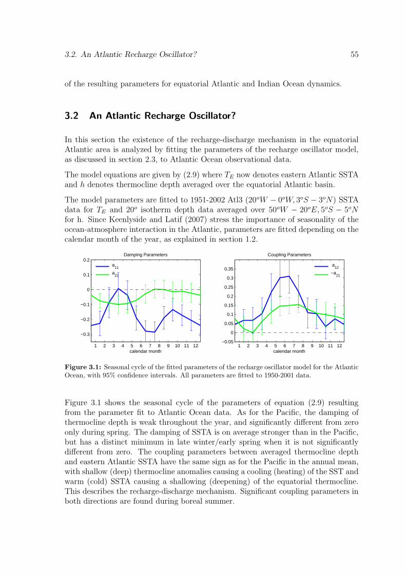
3.2. An Atlantic Recharge Oscillator? 55
of the resulting parameters for equatorial Atlantic and Indian Ocean dynamics.
3.2 An Atlantic Recharge Oscillator?
In this section the existence of the recharge-discharge mechanism in the equatorialAtlantic area is analyzed by fitting the parameters of the recharge oscillator model,as discussed in section 2.3, to Atlantic Ocean observational data.
The model equations are given by (2.9) where TE now denotes eastern Atlantic SSTAand h denotes thermocline depth averaged over the equatorial Atlantic basin.
The model parameters are fitted to 1951-2002 Atl3 (20oW − 0oW, 3oS − 3oN) SSTAdata for TE and 20o isotherm depth data averaged over 50oW − 20oE, 5oS − 5oNfor h. Since Keenlyside and Latif (2007) stress the importance of seasonality of theocean-atmosphere interaction in the Atlantic, parameters are fitted depending on thecalendar month of the year, as explained in section 1.2.
1 2 3 4 5 6 7 8 9 10 11 12
−0.3
−0.2
−0.1
0
0.1
0.2Damping Parameters
calendar month
a
11
a22
1 2 3 4 5 6 7 8 9 10 11 12−0.05
0
0.05
0.1
0.15
0.2
0.25
0.3
0.35
Coupling Parameters
calendar month
a
12
−a21
Figure 3.1: Seasonal cycle of the fitted parameters of the recharge oscillator model for the AtlanticOcean, with 95% confidence intervals. All parameters are fitted to 1950-2001 data.
Figure 3.1 shows the seasonal cycle of the parameters of equation (2.9) resultingfrom the parameter fit to Atlantic Ocean data. As for the Pacific, the damping ofthermocline depth is weak throughout the year, and significantly different from zeroonly during spring. The damping of SSTA is on average stronger than in the Pacific,but has a distinct minimum in late winter/early spring when it is not significantlydifferent from zero. The coupling parameters between averaged thermocline depthand eastern Atlantic SSTA have the same sign as for the Pacific in the annual mean,with shallow (deep) thermocline anomalies causing a cooling (heating) of the SST andwarm (cold) SSTA causing a shallowing (deepening) of the equatorial thermocline.This describes the recharge-discharge mechanism. Significant coupling parameters inboth directions are found during boreal summer.
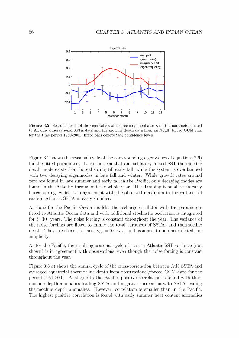
56 CHAPTER 3. ATLANTIC AND INDIAN OCEAN
1 2 3 4 5 6 7 8 9 10 11 12
−0.2
−0.1
0
0.1
0.2
0.3
0.4Eigenvalues
calendar month
real part (growth rate) imaginary part (eigenfrequency)
Figure 3.2: Seasonal cycle of the eigenvalues of the recharge oscillator with the parameters fittedto Atlantic observational SSTA data and thermocline depth data from an NCEP forced GCM run,for the time period 1950-2001. Error bars denote 95% confidence levels.
Figure 3.2 shows the seasonal cycle of the corresponding eigenvalues of equation (2.9)for the fitted parameters. It can be seen that an oscillatory mixed SST-thermoclinedepth mode exists from boreal spring till early fall, while the system is overdampedwith two decaying eigenmodes in late fall and winter. While growth rates aroundzero are found in late summer and early fall in the Pacific, only decaying modes arefound in the Atlantic throughout the whole year. The damping is smallest in earlyboreal spring, which is in agreement with the observed maximum in the variance ofeastern Atlantic SSTA in early summer.
As done for the Pacific Ocean models, the recharge oscillator with the parametersfitted to Atlantic Ocean data and with additional stochastic excitation is integratedfor 3 · 104 years. The noise forcing is constant throughout the year. The variance ofthe noise forcings are fitted to mimic the total variances of SSTAs and thermoclinedepth. They are chosen to meet σξh
= 0.6 · σξTand assumed to be uncorrelated, for
simplicity.
As for the Pacific, the resulting seasonal cycle of eastern Atlantic SST variance (notshown) is in agreement with observations, even though the noise forcing is constantthroughout the year.
Figure 3.3 a) shows the annual cycle of the cross-correlation between Atl3 SSTA andaveraged equatorial thermocline depth from observational/forced GCM data for theperiod 1951-2001. Analogue to the Pacific, positive correlation is found with ther-mocline depth anomalies leading SSTA and negative correlation with SSTA leadingthermocline depth anomalies. However, correlation is smaller than in the Pacific.The highest positive correlation is found with early summer heat content anomalies
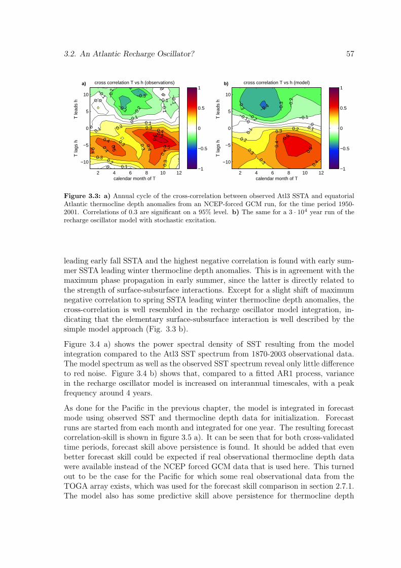
3.2. An Atlantic Recharge Oscillator? 57
−0.2
−0.2
−0.1
−0.1
−0.1
0
0
0
0.10.1
0.1
0.2
0.2
0.3 0.3
0.3
0.3
0.30.
4
0.4
0.4
0.5
0.50.4
0.4
−0.100
−0.3
−0.3
0.6
−0.1
0.4
0.5
0
0
cross correlation T vs h (observations)
calendar month of T
T la
gs h
T
lead
s h
a)
2 4 6 8 10 12
−10
−5
0
5
10
−1
−0.5
0
0.5
1
−0.3
−0.
3
−0.2
−0.
2
−0.1 −0.10
0
0.1
0.1
0.2
0.2
0.3
0.3
0.3
0.4
0.4
0.5
0.5
−0.4
cross correlation T vs h (model)
calendar month of T
T la
gs h
T
lead
s h
b)
2 4 6 8 10 12
−10
−5
0
5
10
−1
−0.5
0
0.5
1
Figure 3.3: a) Annual cycle of the cross-correlation between observed Atl3 SSTA and equatorialAtlantic thermocline depth anomalies from an NCEP-forced GCM run, for the time period 1950-2001. Correlations of 0.3 are significant on a 95% level. b) The same for a 3 · 104 year run of therecharge oscillator model with stochastic excitation.
leading early fall SSTA and the highest negative correlation is found with early sum-mer SSTA leading winter thermocline depth anomalies. This is in agreement with themaximum phase propagation in early summer, since the latter is directly related tothe strength of surface-subsurface interactions. Except for a slight shift of maximumnegative correlation to spring SSTA leading winter thermocline depth anomalies, thecross-correlation is well resembled in the recharge oscillator model integration, in-dicating that the elementary surface-subsurface interaction is well described by thesimple model approach (Fig. 3.3 b).
Figure 3.4 a) shows the power spectral density of SST resulting from the modelintegration compared to the Atl3 SST spectrum from 1870-2003 observational data.The model spectrum as well as the observed SST spectrum reveal only little differenceto red noise. Figure 3.4 b) shows that, compared to a fitted AR1 process, variancein the recharge oscillator model is increased on interannual timescales, with a peakfrequency around 4 years.
As done for the Pacific in the previous chapter, the model is integrated in forecastmode using observed SST and thermocline depth data for initialization. Forecastruns are started from each month and integrated for one year. The resulting forecastcorrelation-skill is shown in figure 3.5 a). It can be seen that for both cross-validatedtime periods, forecast skill above persistence is found. It should be added that evenbetter forecast skill could be expected if real observational thermocline depth datawere available instead of the NCEP forced GCM data that is used here. This turnedout to be the case for the Pacific for which some real observational data from theTOGA array exists, which was used for the forecast skill comparison in section 2.7.1.The model also has some predictive skill above persistence for thermocline depth
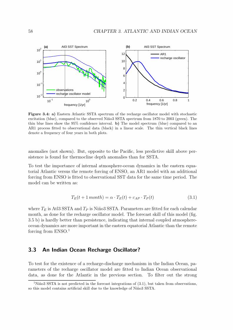
58 CHAPTER 3. ATLANTIC AND INDIAN OCEAN
10−1
100
10−2
10−1
100
101
102
frequency [1/yr]
Atl3 SST Spectrum
(a)
observationsrecharge oscillator model
0.2 0.4 0.6 0.8 10
2
4
6
8
10
12
frequency [1/yr]
Atl3 SST Spectrum
(b)
AR1recharge oscillator
Figure 3.4: a) Eastern Atlantic SSTA spectrum of the recharge oscillator model with stochasticexcitation (blue), compared to the observed Nino3 SSTA spectrum from 1870 to 2003 (green). Thethin blue lines show the 95% confidence interval. b) The model spectrum (blue) compared to anAR1 process fitted to observational data (black) in a linear scale. The thin vertical black linesdenote a frequency of four years in both plots.
anomalies (not shown). But, opposite to the Pacific, less predictive skill above per-sistence is found for thermocline depth anomalies than for SSTA.
To test the importance of internal atmosphere-ocean dynamics in the eastern equa-torial Atlantic versus the remote forcing of ENSO, an AR1 model with an additionalforcing from ENSO is fitted to observational SST data for the same time period. Themodel can be written as:
TE(t + 1 month) = α · TE(t) + cAP · TP (t) (3.1)
where TE is Atl3 SSTA and TP is Nino3 SSTA. Parameters are fitted for each calendarmonth, as done for the recharge oscillator model. The forecast skill of this model (fig.3.5 b) is hardly better than persistence, indicating that internal coupled atmosphere-ocean dynamics are more important in the eastern equatorial Atlantic than the remoteforcing from ENSO.1
3.3 An Indian Ocean Recharge Oscillator?
To test for the existence of a recharge-discharge mechanism in the Indian Ocean, pa-rameters of the recharge oscillator model are fitted to Indian Ocean observationaldata, as done for the Atlantic in the previous section. To filter out the strong
1Nino3 SSTA is not predicted in the forecast integrations of (3.1), but taken from observations,so this model contains artificial skill due to the knowledge of Nino3 SSTA.
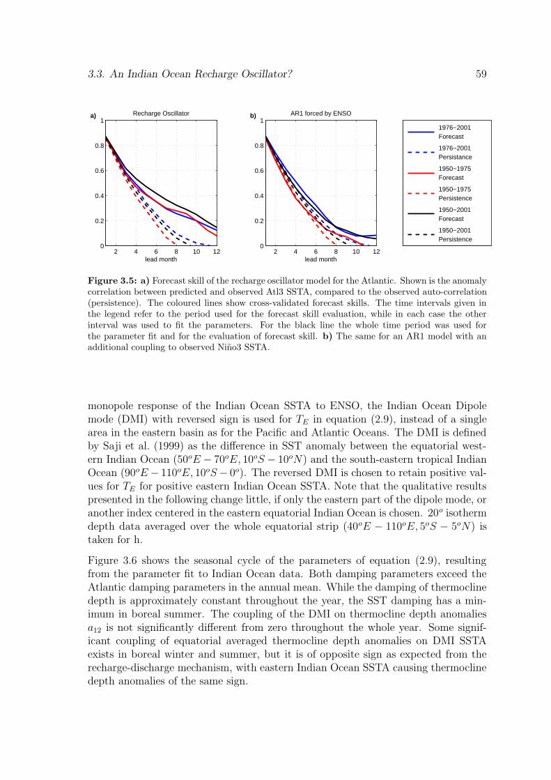
3.3. An Indian Ocean Recharge Oscillator? 59
2 4 6 8 10 120
0.2
0.4
0.6
0.8
1Recharge Oscillator
lead month
a)
2 4 6 8 10 120
0.2
0.4
0.6
0.8
1
lead month
AR1 forced by ENSO
b)
1976−2001 Forecast
1976−2001 Persistance
1950−1975 Forecast
1950−1975 Persistence
1950−2001 Forecast
1950−2001 Persistence
Figure 3.5: a) Forecast skill of the recharge oscillator model for the Atlantic. Shown is the anomalycorrelation between predicted and observed Atl3 SSTA, compared to the observed auto-correlation(persistence). The coloured lines show cross-validated forecast skills. The time intervals given inthe legend refer to the period used for the forecast skill evaluation, while in each case the otherinterval was used to fit the parameters. For the black line the whole time period was used forthe parameter fit and for the evaluation of forecast skill. b) The same for an AR1 model with anadditional coupling to observed Nino3 SSTA.
monopole response of the Indian Ocean SSTA to ENSO, the Indian Ocean Dipolemode (DMI) with reversed sign is used for TE in equation (2.9), instead of a singlearea in the eastern basin as for the Pacific and Atlantic Oceans. The DMI is definedby Saji et al. (1999) as the difference in SST anomaly between the equatorial west-ern Indian Ocean (50oE − 70oE, 10oS − 10oN) and the south-eastern tropical IndianOcean (90oE − 110oE, 10oS − 0o). The reversed DMI is chosen to retain positive val-ues for TE for positive eastern Indian Ocean SSTA. Note that the qualitative resultspresented in the following change little, if only the eastern part of the dipole mode, oranother index centered in the eastern equatorial Indian Ocean is chosen. 20o isothermdepth data averaged over the whole equatorial strip (40oE − 110oE, 5oS − 5oN) istaken for h.
Figure 3.6 shows the seasonal cycle of the parameters of equation (2.9), resultingfrom the parameter fit to Indian Ocean data. Both damping parameters exceed theAtlantic damping parameters in the annual mean. While the damping of thermoclinedepth is approximately constant throughout the year, the SST damping has a min-imum in boreal summer. The coupling of the DMI on thermocline depth anomaliesa12 is not significantly different from zero throughout the whole year. Some signif-icant coupling of equatorial averaged thermocline depth anomalies on DMI SSTAexists in boreal winter and summer, but it is of opposite sign as expected from therecharge-discharge mechanism, with eastern Indian Ocean SSTA causing thermoclinedepth anomalies of the same sign.
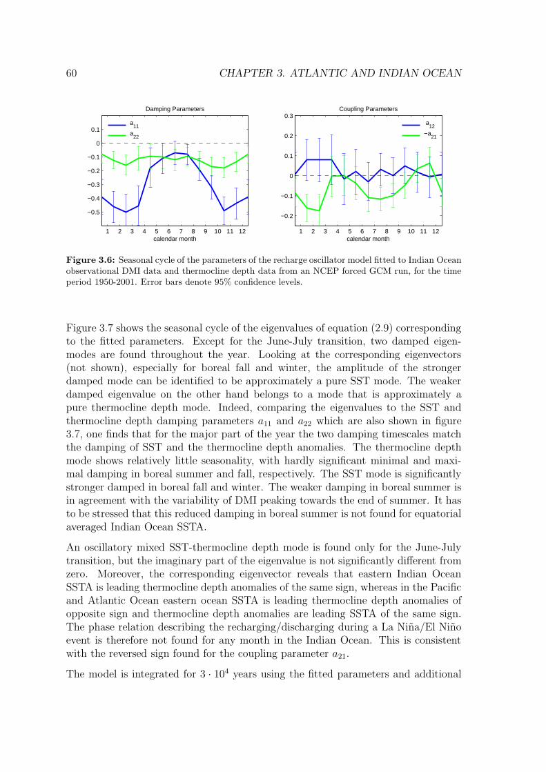
60 CHAPTER 3. ATLANTIC AND INDIAN OCEAN
1 2 3 4 5 6 7 8 9 10 11 12
−0.5
−0.4
−0.3
−0.2
−0.1
0
0.1
Damping Parameters
calendar month
a
11
a22
1 2 3 4 5 6 7 8 9 10 11 12
−0.2
−0.1
0
0.1
0.2
0.3Coupling Parameters
calendar month
a
12
−a21
Figure 3.6: Seasonal cycle of the parameters of the recharge oscillator model fitted to Indian Oceanobservational DMI data and thermocline depth data from an NCEP forced GCM run, for the timeperiod 1950-2001. Error bars denote 95% confidence levels.
Figure 3.7 shows the seasonal cycle of the eigenvalues of equation (2.9) correspondingto the fitted parameters. Except for the June-July transition, two damped eigen-modes are found throughout the year. Looking at the corresponding eigenvectors(not shown), especially for boreal fall and winter, the amplitude of the strongerdamped mode can be identified to be approximately a pure SST mode. The weakerdamped eigenvalue on the other hand belongs to a mode that is approximately apure thermocline depth mode. Indeed, comparing the eigenvalues to the SST andthermocline depth damping parameters a11 and a22 which are also shown in figure3.7, one finds that for the major part of the year the two damping timescales matchthe damping of SST and the thermocline depth anomalies. The thermocline depthmode shows relatively little seasonality, with hardly significant minimal and maxi-mal damping in boreal summer and fall, respectively. The SST mode is significantlystronger damped in boreal fall and winter. The weaker damping in boreal summer isin agreement with the variability of DMI peaking towards the end of summer. It hasto be stressed that this reduced damping in boreal summer is not found for equatorialaveraged Indian Ocean SSTA.
An oscillatory mixed SST-thermocline depth mode is found only for the June-Julytransition, but the imaginary part of the eigenvalue is not significantly different fromzero. Moreover, the corresponding eigenvector reveals that eastern Indian OceanSSTA is leading thermocline depth anomalies of the same sign, whereas in the Pacificand Atlantic Ocean eastern ocean SSTA is leading thermocline depth anomalies ofopposite sign and thermocline depth anomalies are leading SSTA of the same sign.The phase relation describing the recharging/discharging during a La Nina/El Ninoevent is therefore not found for any month in the Indian Ocean. This is consistentwith the reversed sign found for the coupling parameter a21.
The model is integrated for 3 · 104 years using the fitted parameters and additional
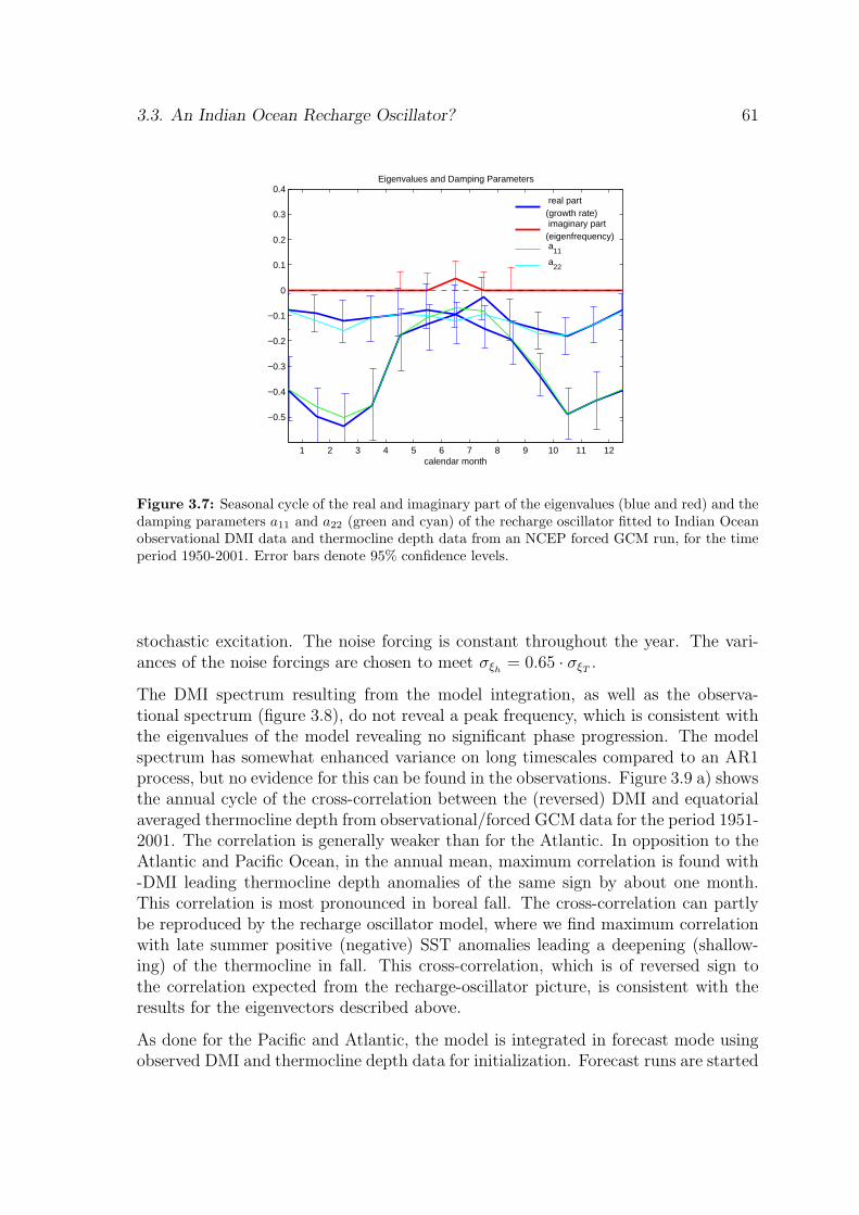
3.3. An Indian Ocean Recharge Oscillator? 61
1 2 3 4 5 6 7 8 9 10 11 12
−0.5
−0.4
−0.3
−0.2
−0.1
0
0.1
0.2
0.3
0.4Eigenvalues and Damping Parameters
calendar month
real part (growth rate) imaginary part (eigenfrequency) a
11
a22
Figure 3.7: Seasonal cycle of the real and imaginary part of the eigenvalues (blue and red) and thedamping parameters a11 and a22 (green and cyan) of the recharge oscillator fitted to Indian Oceanobservational DMI data and thermocline depth data from an NCEP forced GCM run, for the timeperiod 1950-2001. Error bars denote 95% confidence levels.
stochastic excitation. The noise forcing is constant throughout the year. The vari-ances of the noise forcings are chosen to meet σξh
= 0.65 · σξT.
The DMI spectrum resulting from the model integration, as well as the observa-tional spectrum (figure 3.8), do not reveal a peak frequency, which is consistent withthe eigenvalues of the model revealing no significant phase progression. The modelspectrum has somewhat enhanced variance on long timescales compared to an AR1process, but no evidence for this can be found in the observations. Figure 3.9 a) showsthe annual cycle of the cross-correlation between the (reversed) DMI and equatorialaveraged thermocline depth from observational/forced GCM data for the period 1951-2001. The correlation is generally weaker than for the Atlantic. In opposition to theAtlantic and Pacific Ocean, in the annual mean, maximum correlation is found with-DMI leading thermocline depth anomalies of the same sign by about one month.This correlation is most pronounced in boreal fall. The cross-correlation can partlybe reproduced by the recharge oscillator model, where we find maximum correlationwith late summer positive (negative) SST anomalies leading a deepening (shallow-ing) of the thermocline in fall. This cross-correlation, which is of reversed sign tothe correlation expected from the recharge-oscillator picture, is consistent with theresults for the eigenvectors described above.
As done for the Pacific and Atlantic, the model is integrated in forecast mode usingobserved DMI and thermocline depth data for initialization. Forecast runs are started
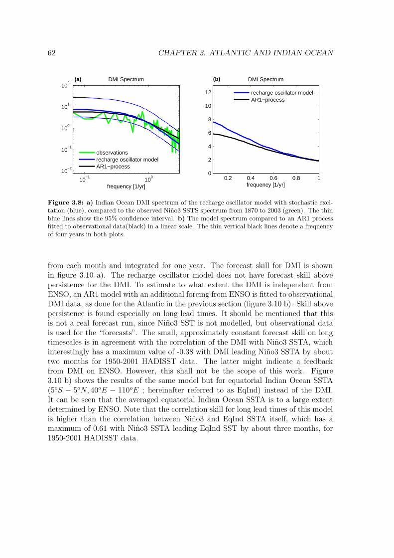
62 CHAPTER 3. ATLANTIC AND INDIAN OCEAN
10−1
100
10−2
10−1
100
101
102
frequency [1/yr]
DMI Spectrum
(a)
observationsrecharge oscillator modelAR1−process
0.2 0.4 0.6 0.8 10
2
4
6
8
10
12
frequency [1/yr]
DMI Spectrum
(b)
recharge oscillator modelAR1−process
Figure 3.8: a) Indian Ocean DMI spectrum of the recharge oscillator model with stochastic exci-tation (blue), compared to the observed Nino3 SSTS spectrum from 1870 to 2003 (green). The thinblue lines show the 95% confidence interval. b) The model spectrum compared to an AR1 processfitted to observational data(black) in a linear scale. The thin vertical black lines denote a frequencyof four years in both plots.
from each month and integrated for one year. The forecast skill for DMI is shownin figure 3.10 a). The recharge oscillator model does not have forecast skill abovepersistence for the DMI. To estimate to what extent the DMI is independent fromENSO, an AR1 model with an additional forcing from ENSO is fitted to observationalDMI data, as done for the Atlantic in the previous section (figure 3.10 b). Skill abovepersistence is found especially on long lead times. It should be mentioned that thisis not a real forecast run, since Nino3 SST is not modelled, but observational datais used for the “forecasts”. The small, approximately constant forecast skill on longtimescales is in agreement with the correlation of the DMI with Nino3 SSTA, whichinterestingly has a maximum value of -0.38 with DMI leading Nino3 SSTA by abouttwo months for 1950-2001 HADISST data. The latter might indicate a feedbackfrom DMI on ENSO. However, this shall not be the scope of this work. Figure3.10 b) shows the results of the same model but for equatorial Indian Ocean SSTA(5oS − 5oN, 40oE − 110oE ; hereinafter referred to as EqInd) instead of the DMI.It can be seen that the averaged equatorial Indian Ocean SSTA is to a large extentdetermined by ENSO. Note that the correlation skill for long lead times of this modelis higher than the correlation between Nino3 and EqInd SSTA itself, which has amaximum of 0.61 with Nino3 SSTA leading EqInd SST by about three months, for1950-2001 HADISST data.
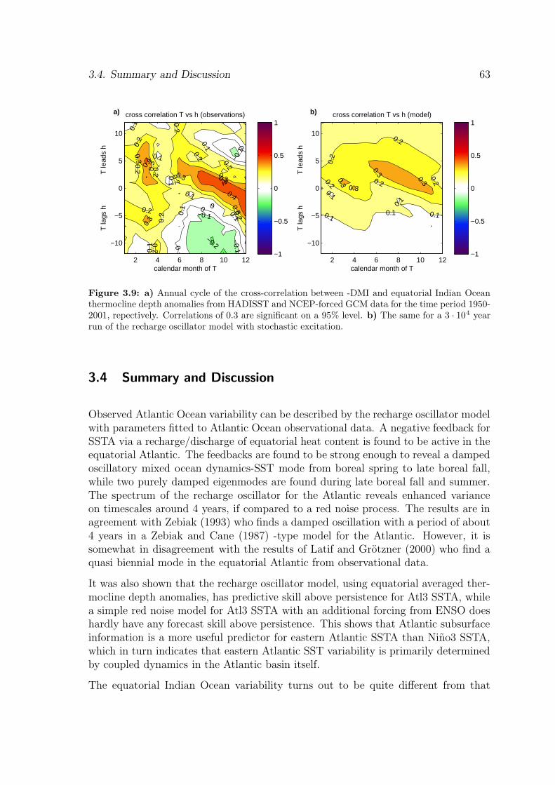
3.4. Summary and Discussion 63
−0.1
−0.1
0
0
0
0.1
0.1
0.10.1
0.1
0.2
0.20.2
0.2
0.2
0.2
0.2
0.2
0.2
0.2
0.3
0.3 0.3
0.4
0.4
0.3
0.3
0.2
−0.1
0.1
0.3
0.1
−0.2
0.1
0.4
0
cross correlation T vs h (observations)
calendar month of T
T la
gs h
T
lead
s h
a)
2 4 6 8 10 12
−10
−5
0
5
10
−1
−0.5
0
0.5
1
0.10.10.1
0.2
0.2
0.20.20.2
0.3
0.3
0.3
0.10.3
0.1
cross correlation T vs h (model)
calendar month of T
T la
gs h
T
lead
s h
b)
2 4 6 8 10 12
−10
−5
0
5
10
−1
−0.5
0
0.5
1
Figure 3.9: a) Annual cycle of the cross-correlation between -DMI and equatorial Indian Oceanthermocline depth anomalies from HADISST and NCEP-forced GCM data for the time period 1950-2001, repectively. Correlations of 0.3 are significant on a 95% level. b) The same for a 3 · 104 yearrun of the recharge oscillator model with stochastic excitation.
3.4 Summary and Discussion
Observed Atlantic Ocean variability can be described by the recharge oscillator modelwith parameters fitted to Atlantic Ocean observational data. A negative feedback forSSTA via a recharge/discharge of equatorial heat content is found to be active in theequatorial Atlantic. The feedbacks are found to be strong enough to reveal a dampedoscillatory mixed ocean dynamics-SST mode from boreal spring to late boreal fall,while two purely damped eigenmodes are found during late boreal fall and summer.The spectrum of the recharge oscillator for the Atlantic reveals enhanced varianceon timescales around 4 years, if compared to a red noise process. The results are inagreement with Zebiak (1993) who finds a damped oscillation with a period of about4 years in a Zebiak and Cane (1987) -type model for the Atlantic. However, it issomewhat in disagreement with the results of Latif and Grotzner (2000) who find aquasi biennial mode in the equatorial Atlantic from observational data.
It was also shown that the recharge oscillator model, using equatorial averaged ther-mocline depth anomalies, has predictive skill above persistence for Atl3 SSTA, whilea simple red noise model for Atl3 SSTA with an additional forcing from ENSO doeshardly have any forecast skill above persistence. This shows that Atlantic subsurfaceinformation is a more useful predictor for eastern Atlantic SSTA than Nino3 SSTA,which in turn indicates that eastern Atlantic SST variability is primarily determinedby coupled dynamics in the Atlantic basin itself.
The equatorial Indian Ocean variability turns out to be quite different from that
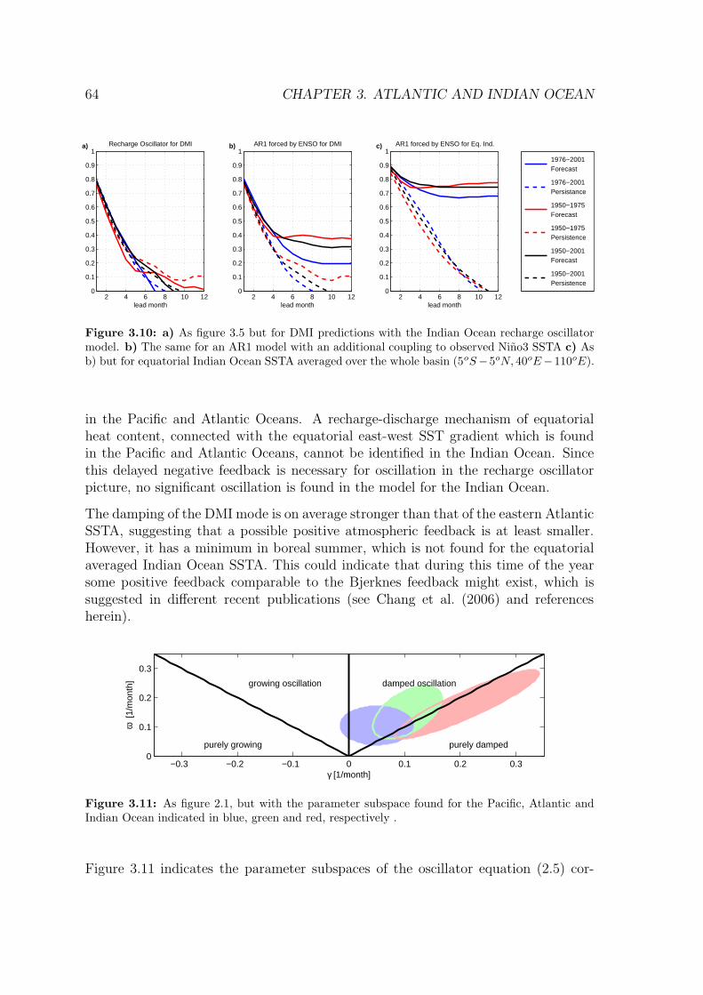
64 CHAPTER 3. ATLANTIC AND INDIAN OCEAN
2 4 6 8 10 120
0.1
0.2
0.3
0.4
0.5
0.6
0.7
0.8
0.9
1Recharge Oscillator for DMI
lead month
a)
2 4 6 8 10 120
0.1
0.2
0.3
0.4
0.5
0.6
0.7
0.8
0.9
1AR1 forced by ENSO for DMI
lead month
b)
2 4 6 8 10 120
0.1
0.2
0.3
0.4
0.5
0.6
0.7
0.8
0.9
1
lead month
AR1 forced by ENSO for Eq. Ind.
c)
1976−2001 Forecast
1976−2001 Persistance
1950−1975 Forecast
1950−1975 Persistence
1950−2001 Forecast
1950−2001 Persistence
Figure 3.10: a) As figure 3.5 but for DMI predictions with the Indian Ocean recharge oscillatormodel. b) The same for an AR1 model with an additional coupling to observed Nino3 SSTA c) Asb) but for equatorial Indian Ocean SSTA averaged over the whole basin (5oS−5oN, 40oE−110oE).
in the Pacific and Atlantic Oceans. A recharge-discharge mechanism of equatorialheat content, connected with the equatorial east-west SST gradient which is foundin the Pacific and Atlantic Oceans, cannot be identified in the Indian Ocean. Sincethis delayed negative feedback is necessary for oscillation in the recharge oscillatorpicture, no significant oscillation is found in the model for the Indian Ocean.
The damping of the DMI mode is on average stronger than that of the eastern AtlanticSSTA, suggesting that a possible positive atmospheric feedback is at least smaller.However, it has a minimum in boreal summer, which is not found for the equatorialaveraged Indian Ocean SSTA. This could indicate that during this time of the yearsome positive feedback comparable to the Bjerknes feedback might exist, which issuggested in different recent publications (see Chang et al. (2006) and referencesherein).
−0.3 −0.2 −0.1 0 0.1 0.2 0.30
0.1
0.2
0.3
γ [1/month]
ω [
1/m
onth
]
purely growing purely damped
growing oscillation damped oscillation
Figure 3.11: As figure 2.1, but with the parameter subspace found for the Pacific, Atlantic andIndian Ocean indicated in blue, green and red, respectively .
Figure 3.11 indicates the parameter subspaces of the oscillator equation (2.5) cor-
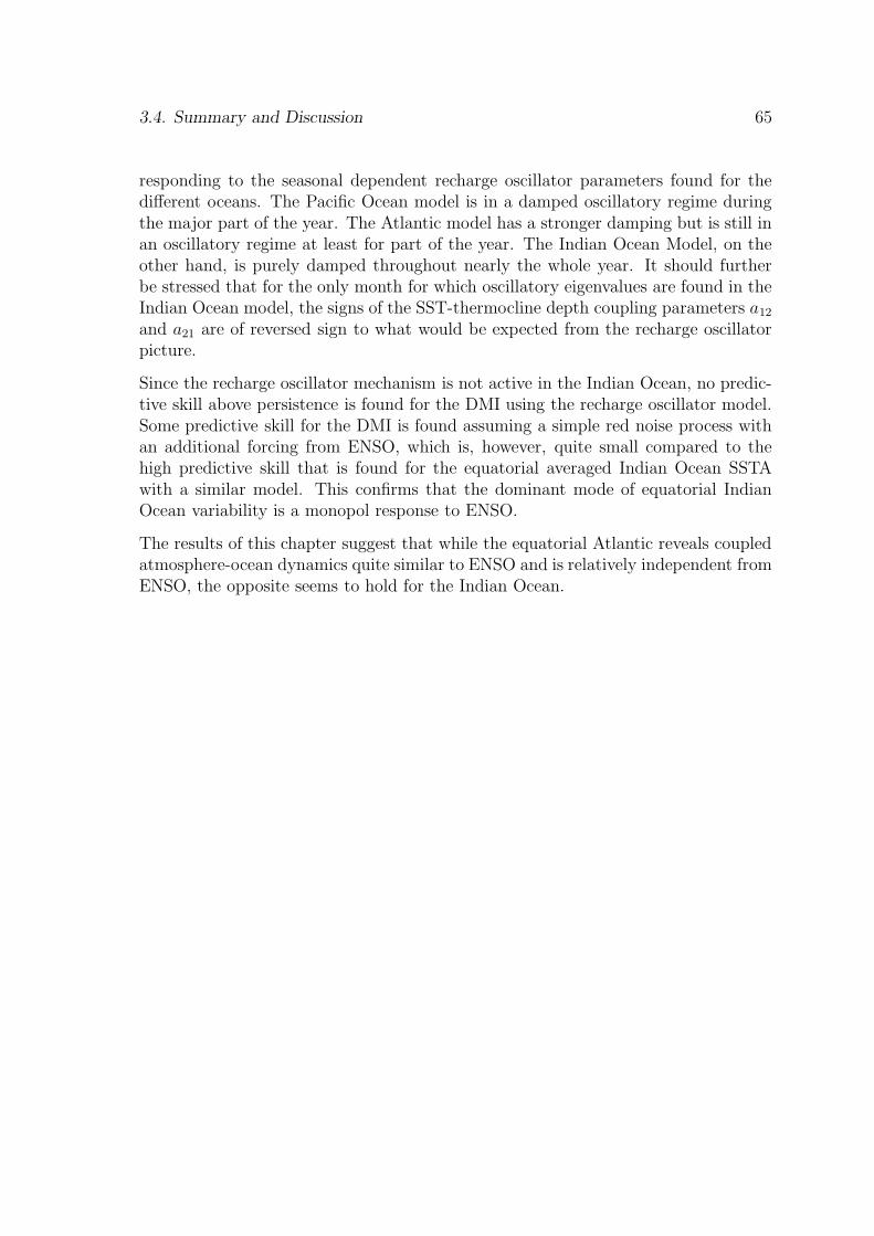
3.4. Summary and Discussion 65
responding to the seasonal dependent recharge oscillator parameters found for thedifferent oceans. The Pacific Ocean model is in a damped oscillatory regime duringthe major part of the year. The Atlantic model has a stronger damping but is still inan oscillatory regime at least for part of the year. The Indian Ocean Model, on theother hand, is purely damped throughout nearly the whole year. It should furtherbe stressed that for the only month for which oscillatory eigenvalues are found in theIndian Ocean model, the signs of the SST-thermocline depth coupling parameters a12
and a21 are of reversed sign to what would be expected from the recharge oscillatorpicture.
Since the recharge oscillator mechanism is not active in the Indian Ocean, no predic-tive skill above persistence is found for the DMI using the recharge oscillator model.Some predictive skill for the DMI is found assuming a simple red noise process withan additional forcing from ENSO, which is, however, quite small compared to thehigh predictive skill that is found for the equatorial averaged Indian Ocean SSTAwith a similar model. This confirms that the dominant mode of equatorial IndianOcean variability is a monopol response to ENSO.
The results of this chapter suggest that while the equatorial Atlantic reveals coupledatmosphere-ocean dynamics quite similar to ENSO and is relatively independent fromENSO, the opposite seems to hold for the Indian Ocean.
Chapter 4
Tropical Oceans’ Interaction
4.1 Introduction
While it is known that the Indian Ocean shows a strong response to ENSO (e.g.Venzke et al. (2000)), more recently, different studies also suggest a feedback of theIndian Ocean SSTA on ENSO. Analyzing observational data, Kug and Kang (2006)suggest a negative feedback of the tropical Indian Ocean on ENSO, with a warmIndian Ocean causing a decay of ENSO events via anomalous easterly winds in thewestern Pacific. CGCM experiments on the influence of the Indian Ocean on theENSO cycle come to somewhat controversial results. Yu et al. (2002) find that ENSOvariability is decreased and the frequency is slightly increased from a 4.4 to a 4 yearsperiod in a 42 year model integration, if the Indian Ocean is decoupled from thesystem. Wu and Kirtman (2004) agree that ENSO variability is decreased, but findthat the frequency is also decreased if the Indian Ocean is decoupled. Dommengetet al. (2006) agree with the latter that the ENSO frequency is decreased, but findincreased ENSO variability if the Indian Ocean is decoupled from the system.
While there is general agreement that the Atlantic sector is influenced by ENSO,with a particular strong response in the western subtropical Atlantic, some disagree-ment on the equatorial Atlantic’s response to remote ENSO forcing exists. The weakinstantaneous correlation between equatorial Atlantic and Nino3 SSTA has led tothe suggestion that ENSO has no significant influence on the equatorial Atlantic (Ze-biak (1993), Enfield and Mayer (1997)). However, seasonally stratified correlations,lag regressions and composite analyses come to conflicting results, concerning theresponse of equatorial Atlantic SST on ENSO (e.g. Saravanan and Chang (2000),Ruiz-Barradas et al. (2000), Huang (2004), Latif and Grotzner (2000)). Recently,Keenlyside and Latif (2007) stress a maximum negative correlation between Nino3SSTA and eastern equatorial Atlantic SSTA with Atl3 leading Nino3 SSTA by about6 months. This indicates a feedback from the Atlantic on ENSO, rising hope thatENSO predictions can be improved by explicitly including Atlantic SSTA.
66
4.2. A Simple Model for the Tropical Oceans’ Interactions with ENSO 67
Here, simple models are proposed as hypotheses for the interaction of the tropicalAtlantic and Indian Oceans with ENSO. As in the previous chapters, the modelparameters are fitted to observational data and the implications of the resultingparameters for the impact of the Indian and Atlantic Ocean on the ENSO cycle areanalyzed. In the picture of this conceptual model, the different results of the CGCMstudies for the influence of the Indian Ocean on the ENSO cycle can be explained onthe basis of the biases of the CGCMs. Finally, a simple model including interactionsbetween all tropical Oceans is proposed.
4.2 A Simple Model for the Tropical Oceans’ Interactions withENSO
A simple coupled model for the interactions of the Pacific and the Atlantic or IndianOcean is proposed by Dommenget et al. (2006). It consists of the simplest rechargeoscillator model suggested by Burgers et al. (2005) coupled to a linear damping modelfor the Atlantic/Indian Ocean. It proposes a feedback from the Atlantic/Indian Oceanon Pacific SST. Kug and Kang (2006) propose a similar model but with a feedbackon western equatorial thermocline depth. In the following, the model as used byDommenget et al. (2006) is extended by a feedback of Indian/Atlantic Ocean SSTAon averaged Pacific thermocline depth. It can be written as
ddt
TP = ω0hP − 2γPTP + cPI/PATI/A + ξP
ddt
hP = −ω0TP + chPI/PATI/A + ξh
ddt
TI/A = −2γI/ATI/A + cIP/AP TP + ξI/A
(4.1)
where TP is eastern Pacific (Nino3) SSTA, hp denotes thermocline depth anomalyaveraged over the equatorial Pacific and TI/A is equatorial Indian/Atlantic OceanSSTA. The cIP/AP term describes the coupling of the Indian/Atlantic Ocean to PacificSSTA whereas cPI/PA and chPI/PA represent the feedback of Indian/Atlantic OceanSSTA on Pacific SST and thermocline depth, respectively. ξTP
, ξh and ξTI/A againdenote stochastic excitation, representing wind and heat flux forcing due to shorttime scale uncoupled atmospheric variability.
4.3 Indian Ocean-ENSO Interaction
The parameters of (4.1) are fitted to 1951-2002 EqInd and Nino3 SSTA data and20o isotherm depth data averaged over 120oE − 80oW, 5oS − 5oN for h. The dataand fitting methods are described in chapter 1. To constrain the number of degrees
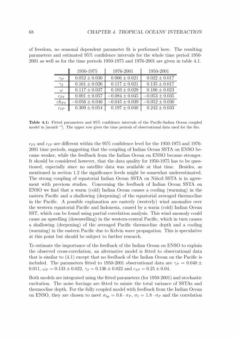
68 CHAPTER 4. TROPICAL OCEANS’ INTERACTION
of freedom, no seasonal dependent parameter fit is performed here. The resultingparameters and estimated 95% confidence intervals for the whole time period 1950-2001 as well as for the time periods 1950-1975 and 1976-2001 are given in table 4.1.
1950-1975 1976-2001 1950-2001
γP 0.052 ± 0.030 0.006 ± 0.021 0.022 ± 0.017γI 0.161 ± 0.026 0.117 ± 0.021 0.135 ± 0.017ω 0.117 ± 0.037 0.103 ± 0.029 0.106 ± 0.023
cPI 0.001 ± 0.057 −0.084 ± 0.045 −0.053 ± 0.035chPI −0.056 ± 0.046 −0.045 ± 0.039 −0.052 ± 0.030cIP 0.309 ± 0.054 0.197 ± 0.040 0.242 ± 0.033
Table 4.1: Fitted parameters and 95% confidence intervals of the Pacific-Indian Ocean coupledmodel in [month−1]. The upper row gives the time periods of observational data used for the fits.
cPI and cIP are different within the 95% confidence level for the 1950-1975 and 1976-2001 time periods, suggesting that the coupling of Indian Ocean SSTA on ENSO be-came weaker, while the feedback from the Indian Ocean on ENSO became stronger.It should be considered however, that the data quality for 1950-1975 has to be ques-tioned, especially since no satellite data was available at that time. Besides, asmentioned in section 1.2 the significance levels might be somewhat underestimated.The strong coupling of equatorial Indian Ocean SSTA on Nino3 SSTA is in agree-ment with previous studies. Concerning the feedback of Indian Ocean SSTA onENSO we find that a warm (cold) Indian Ocean causes a cooling (warming) in theeastern Pacific and a shallowing (deepening) of the equatorial averaged thermoclinein the Pacific. A possible explanation are easterly (westerly) wind anomalies overthe western equatorial Pacific and Indonesia, caused by a warm (cold) Indian OceanSST, which can be found using partial correlation analysis. This wind anomaly couldcause an upwelling (downwelling) in the western-central Pacific, which in turn causesa shallowing (deepening) of the averaged Pacific thermocline depth and a cooling(warming) in the eastern Pacific due to Kelvin wave propagation. This is speculativeat this point but should be subject to further research.
To estimate the importance of the feedback of the Indian Ocean on ENSO to explainthe observed cross-correlation, an alternative model is fitted to observational datathat is similar to (4.1) except that no feedback of the Indian Ocean on the Pacific isincluded. The parameters fitted to 1950-2001 observational data are γP = 0.040 ±0.011, ωP = 0.133 ± 0.022, γI = 0.136 ± 0.022 and cIP = 0.25 ± 0.04.
Both models are integrated using the fitted parameters (for 1950-2001) and stochasticexcitation. The noise forcings are fitted to mimic the total variance of SSTAs andthermocline depth. For the fully coupled model with feedback from the Indian Oceanon ENSO, they are chosen to meet σhp = 0.6 · σP , σI = 1.8 · σP and the correlation
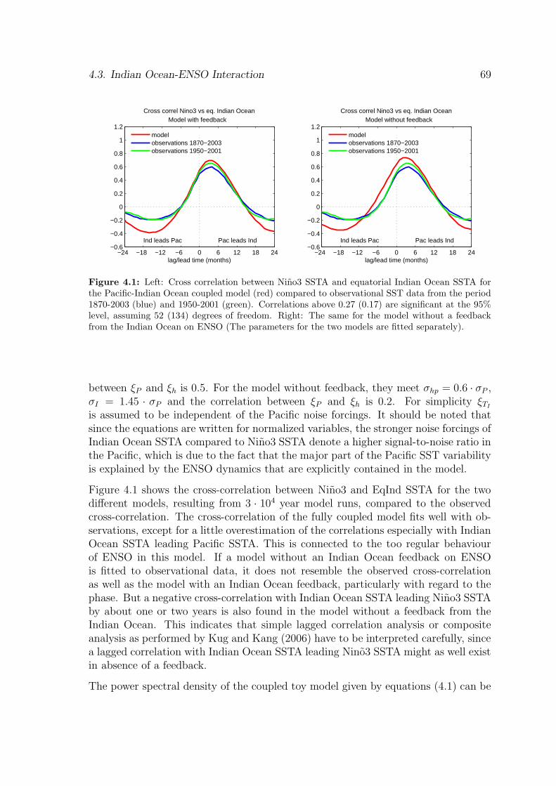
4.3. Indian Ocean-ENSO Interaction 69
−24 −18 −12 −6 0 6 12 18 24−0.6
−0.4
−0.2
0
0.2
0.4
0.6
0.8
1
1.2
Cross correl Nino3 vs eq. Indian Ocean Model with feedback
Ind leads Pac Pac leads Ind
lag/lead time (months)
modelobservations 1870−2003observations 1950−2001
−24 −18 −12 −6 0 6 12 18 24−0.6
−0.4
−0.2
0
0.2
0.4
0.6
0.8
1
1.2
Cross correl Nino3 vs eq. Indian Ocean Model without feedback
Ind leads Pac Pac leads Ind
lag/lead time (months)
modelobservations 1870−2003observations 1950−2001
Figure 4.1: Left: Cross correlation between Nino3 SSTA and equatorial Indian Ocean SSTA forthe Pacific-Indian Ocean coupled model (red) compared to observational SST data from the period1870-2003 (blue) and 1950-2001 (green). Correlations above 0.27 (0.17) are significant at the 95%level, assuming 52 (134) degrees of freedom. Right: The same for the model without a feedbackfrom the Indian Ocean on ENSO (The parameters for the two models are fitted separately).
between ξP and ξh is 0.5. For the model without feedback, they meet σhp = 0.6 · σP ,σI = 1.45 · σP and the correlation between ξP and ξh is 0.2. For simplicity ξTI
is assumed to be independent of the Pacific noise forcings. It should be noted thatsince the equations are written for normalized variables, the stronger noise forcings ofIndian Ocean SSTA compared to Nino3 SSTA denote a higher signal-to-noise ratio inthe Pacific, which is due to the fact that the major part of the Pacific SST variabilityis explained by the ENSO dynamics that are explicitly contained in the model.
Figure 4.1 shows the cross-correlation between Nino3 and EqInd SSTA for the twodifferent models, resulting from 3 · 104 year model runs, compared to the observedcross-correlation. The cross-correlation of the fully coupled model fits well with ob-servations, except for a little overestimation of the correlations especially with IndianOcean SSTA leading Pacific SSTA. This is connected to the too regular behaviourof ENSO in this model. If a model without an Indian Ocean feedback on ENSOis fitted to observational data, it does not resemble the observed cross-correlationas well as the model with an Indian Ocean feedback, particularly with regard to thephase. But a negative cross-correlation with Indian Ocean SSTA leading Nino3 SSTAby about one or two years is also found in the model without a feedback from theIndian Ocean. This indicates that simple lagged correlation analysis or compositeanalysis as performed by Kug and Kang (2006) have to be interpreted carefully, sincea lagged correlation with Indian Ocean SSTA leading Nino3 SSTA might as well existin absence of a feedback.
The power spectral density of the coupled toy model given by equations (4.1) can be
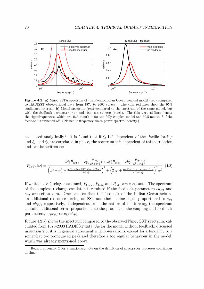
70 CHAPTER 4. TROPICAL OCEANS’ INTERACTION
10−1
100
0
0.1
0.2
0.3
0.4
0.5
0.6
0.7
0.8
frequency (yr−1)
varia
nce
Nino3 SST
(a) observed spectrum model spectrum
10−1
100
0
0.2
0.4
0.6
0.8
1
frequency (yr−1)
varia
nce
Nino3 SST − feedback
(b)with feedbackno feedback
Figure 4.2: a) Nino3 SSTA spectrum of the Pacific-Indian Ocean coupled model (red) comparedto HADISST observational data from 1870 to 2003 (black). The thin red lines show the 95%confidence interval. b) Model spectrum (red) compared to the spectrum of the same model, butwith the feedback parameters cPI and chPI set to zero (black). The thin vertical lines denotethe eigenfrequencies, which are 48.5 month−1 for the fully coupled model and 60.5 month−1 if thefeedback is switched off. (Plotted is frequency times power spectral density.)
calculated analytically.1 It is found that if ξI is independent of the Pacific forcingand ξT and ξh are correlated in phase, the spectrum is independent of this correlationand can be written as:
PTP TP(ω) =
ω2(PξP ξP+ c2
PI
PξIξI
ω2+4γ2
I
) + ω20(Pξhξh
+ ch2PI
PξI ξI
ω2+4γ2
I
)(
ω2 − ω20 + ω2cIP cPI+2γIω0cIP chPI
ω2+4γ2
I
)2+(
2γP + ω0chPIcIP−2γIcPIcIP
ω2+4γ2
I
)2ω2
(4.2)
If white noise forcing is assumed, PξP ξP, Pξhξh
and PξIξIare constants. The spectrum
of the simplest recharge oscillator is retained if the feedback parameters chPI andcPI are set to zero. One can see that the feedback of the Indian Ocean acts asan additional red noise forcing on SST and thermocline depth proportional to cPI
and chPI , respectively. Independent from the nature of the forcing, the spectrumcontains additional terms proportional to the product of the coupling and feedbackparameters, cIP cPI or cIP chPI.
Figure 4.2 a) shows the spectrum compared to the observed Nino3 SST spectrum, cal-culated from 1870-2003 HADISST data. As for the model without feedback, discussedin section 2.3, it is in general agreement with observations, except for a tendency to asomewhat too pronounced peak and therefore a too regular behaviour in the model,which was already mentioned above.
1Regard appendix C for a cautionary note on the definition of spectra for processes continuousin time.
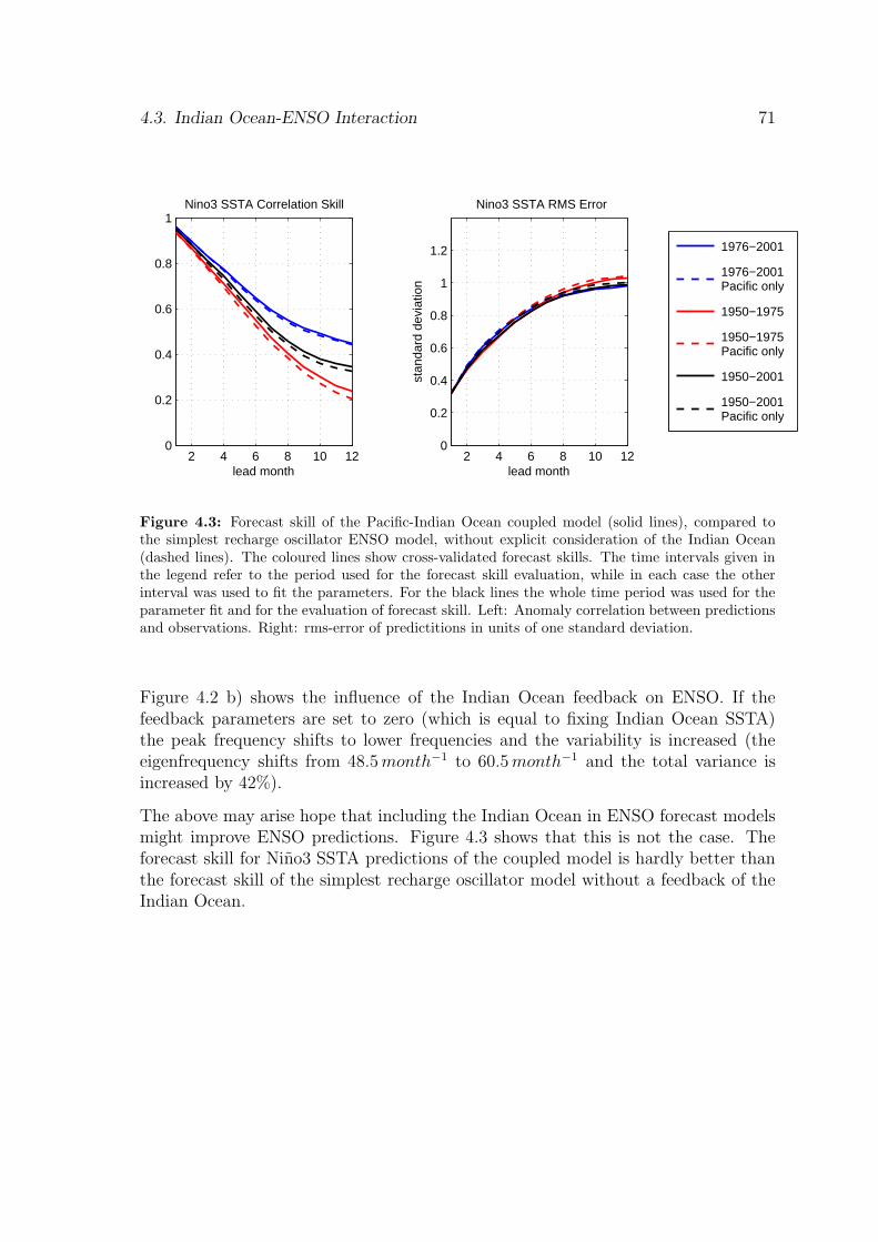
4.3. Indian Ocean-ENSO Interaction 71
2 4 6 8 10 120
0.2
0.4
0.6
0.8
1
lead month
Nino3 SSTA Correlation Skill
1976−2001
1976−2001 Pacific only
1950−1975
1950−1975 Pacific only
1950−2001
1950−2001 Pacific only
2 4 6 8 10 120
0.2
0.4
0.6
0.8
1
1.2
Nino3 SSTA RMS Error
lead month
stan
dard
dev
iatio
n
Figure 4.3: Forecast skill of the Pacific-Indian Ocean coupled model (solid lines), compared tothe simplest recharge oscillator ENSO model, without explicit consideration of the Indian Ocean(dashed lines). The coloured lines show cross-validated forecast skills. The time intervals given inthe legend refer to the period used for the forecast skill evaluation, while in each case the otherinterval was used to fit the parameters. For the black lines the whole time period was used for theparameter fit and for the evaluation of forecast skill. Left: Anomaly correlation between predictionsand observations. Right: rms-error of predictitions in units of one standard deviation.
Figure 4.2 b) shows the influence of the Indian Ocean feedback on ENSO. If thefeedback parameters are set to zero (which is equal to fixing Indian Ocean SSTA)the peak frequency shifts to lower frequencies and the variability is increased (theeigenfrequency shifts from 48.5 month−1 to 60.5 month−1 and the total variance isincreased by 42%).
The above may arise hope that including the Indian Ocean in ENSO forecast modelsmight improve ENSO predictions. Figure 4.3 shows that this is not the case. Theforecast skill for Nino3 SSTA predictions of the coupled model is hardly better thanthe forecast skill of the simplest recharge oscillator model without a feedback of theIndian Ocean.
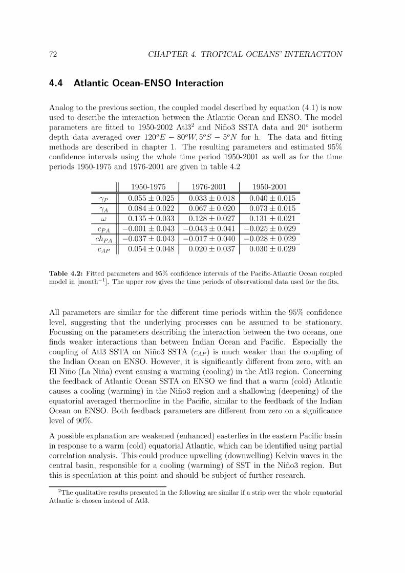
72 CHAPTER 4. TROPICAL OCEANS’ INTERACTION
4.4 Atlantic Ocean-ENSO Interaction
Analog to the previous section, the coupled model described by equation (4.1) is nowused to describe the interaction between the Atlantic Ocean and ENSO. The modelparameters are fitted to 1950-2002 Atl32 and Nino3 SSTA data and 20o isothermdepth data averaged over 120oE − 80oW, 5oS − 5oN for h. The data and fittingmethods are described in chapter 1. The resulting parameters and estimated 95%confidence intervals using the whole time period 1950-2001 as well as for the timeperiods 1950-1975 and 1976-2001 are given in table 4.2
1950-1975 1976-2001 1950-2001
γP 0.055 ± 0.025 0.033 ± 0.018 0.040 ± 0.015γA 0.084 ± 0.022 0.067 ± 0.020 0.073 ± 0.015ω 0.135 ± 0.033 0.128 ± 0.027 0.131 ± 0.021
cPA −0.001 ± 0.043 −0.043 ± 0.041 −0.025 ± 0.029chPA −0.037 ± 0.043 −0.017 ± 0.040 −0.028 ± 0.029cAP 0.054 ± 0.048 0.020 ± 0.037 0.030 ± 0.029
Table 4.2: Fitted parameters and 95% confidence intervals of the Pacific-Atlantic Ocean coupledmodel in [month−1]. The upper row gives the time periods of observational data used for the fits.
All parameters are similar for the different time periods within the 95% confidencelevel, suggesting that the underlying processes can be assumed to be stationary.Focussing on the parameters describing the interaction between the two oceans, onefinds weaker interactions than between Indian Ocean and Pacific. Especially thecoupling of Atl3 SSTA on Nino3 SSTA (cAP ) is much weaker than the coupling ofthe Indian Ocean on ENSO. However, it is significantly different from zero, with anEl Nino (La Nina) event causing a warming (cooling) in the Atl3 region. Concerningthe feedback of Atlantic Ocean SSTA on ENSO we find that a warm (cold) Atlanticcauses a cooling (warming) in the Nino3 region and a shallowing (deepening) of theequatorial averaged thermocline in the Pacific, similar to the feedback of the IndianOcean on ENSO. Both feedback parameters are different from zero on a significancelevel of 90%.
A possible explanation are weakened (enhanced) easterlies in the eastern Pacific basinin response to a warm (cold) equatorial Atlantic, which can be identified using partialcorrelation analysis. This could produce upwelling (downwelling) Kelvin waves in thecentral basin, responsible for a cooling (warming) of SST in the Nino3 region. Butthis is speculation at this point and should be subject of further research.
2The qualitative results presented in the following are similar if a strip over the whole equatorialAtlantic is chosen instead of Atl3.
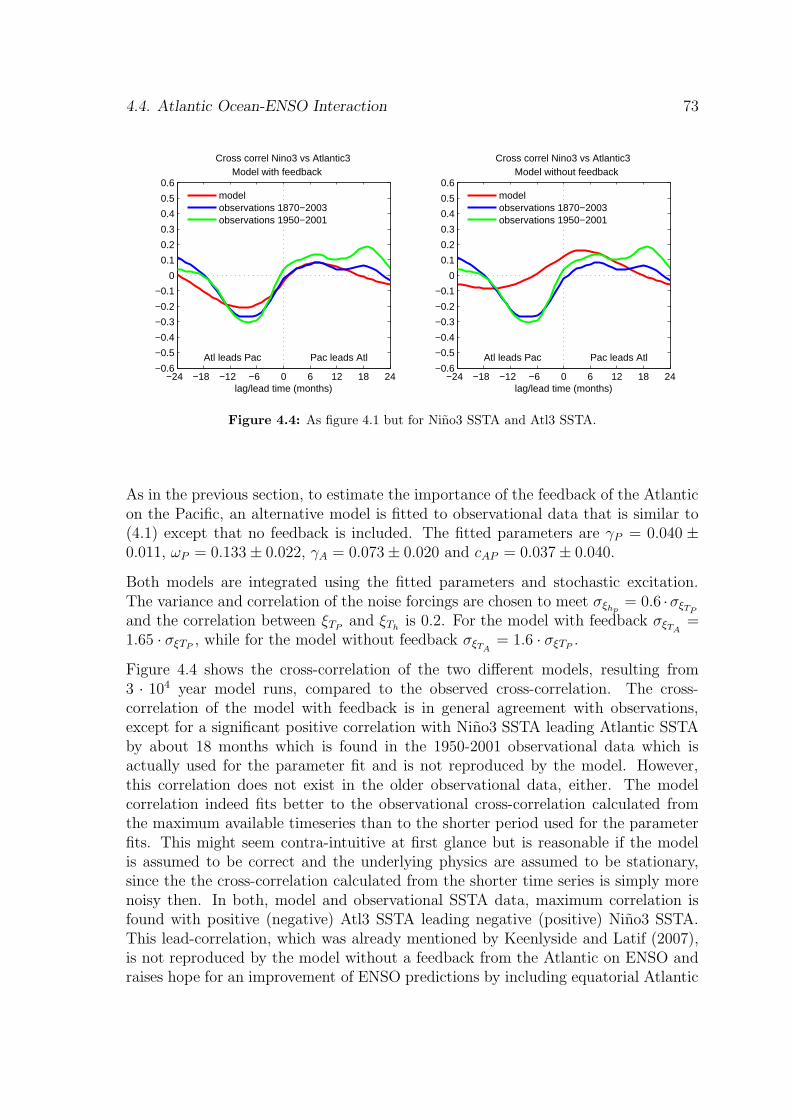
4.4. Atlantic Ocean-ENSO Interaction 73
−24 −18 −12 −6 0 6 12 18 24−0.6
−0.5
−0.4
−0.3
−0.2
−0.1
0
0.1
0.2
0.3
0.4
0.5
0.6
Cross correl Nino3 vs Atlantic3 Model with feedback
Atl leads Pac Pac leads Atl
lag/lead time (months)
modelobservations 1870−2003observations 1950−2001
−24 −18 −12 −6 0 6 12 18 24−0.6
−0.5
−0.4
−0.3
−0.2
−0.1
0
0.1
0.2
0.3
0.4
0.5
0.6
Cross correl Nino3 vs Atlantic3 Model without feedback
Atl leads Pac Pac leads Atl
lag/lead time (months)
modelobservations 1870−2003observations 1950−2001
Figure 4.4: As figure 4.1 but for Nino3 SSTA and Atl3 SSTA.
As in the previous section, to estimate the importance of the feedback of the Atlanticon the Pacific, an alternative model is fitted to observational data that is similar to(4.1) except that no feedback is included. The fitted parameters are γP = 0.040 ±0.011, ωP = 0.133 ± 0.022, γA = 0.073 ± 0.020 and cAP = 0.037 ± 0.040.
Both models are integrated using the fitted parameters and stochastic excitation.The variance and correlation of the noise forcings are chosen to meet σξhp
= 0.6 ·σξTP
and the correlation between ξTPand ξTh
is 0.2. For the model with feedback σξTA=
1.65 · σξTP, while for the model without feedback σξTA
= 1.6 · σξTP.
Figure 4.4 shows the cross-correlation of the two different models, resulting from3 · 104 year model runs, compared to the observed cross-correlation. The cross-correlation of the model with feedback is in general agreement with observations,except for a significant positive correlation with Nino3 SSTA leading Atlantic SSTAby about 18 months which is found in the 1950-2001 observational data which isactually used for the parameter fit and is not reproduced by the model. However,this correlation does not exist in the older observational data, either. The modelcorrelation indeed fits better to the observational cross-correlation calculated fromthe maximum available timeseries than to the shorter period used for the parameterfits. This might seem contra-intuitive at first glance but is reasonable if the modelis assumed to be correct and the underlying physics are assumed to be stationary,since the the cross-correlation calculated from the shorter time series is simply morenoisy then. In both, model and observational SSTA data, maximum correlation isfound with positive (negative) Atl3 SSTA leading negative (positive) Nino3 SSTA.This lead-correlation, which was already mentioned by Keenlyside and Latif (2007),is not reproduced by the model without a feedback from the Atlantic on ENSO andraises hope for an improvement of ENSO predictions by including equatorial Atlantic
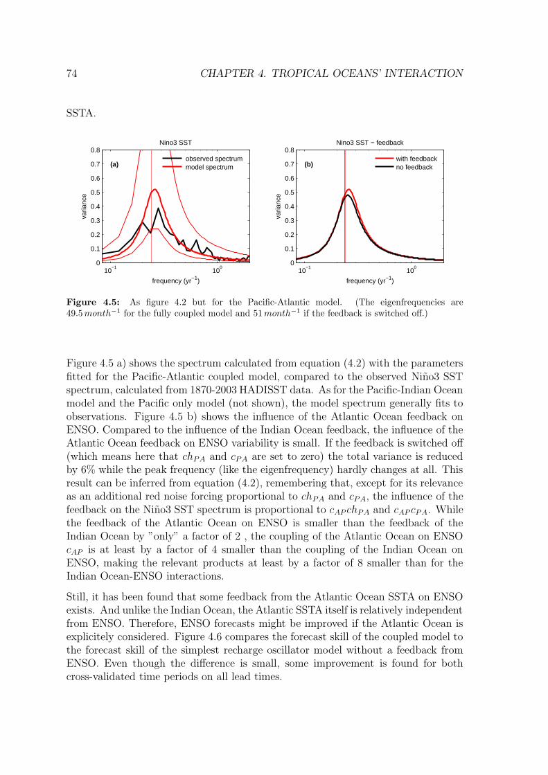
74 CHAPTER 4. TROPICAL OCEANS’ INTERACTION
SSTA.
10−1
100
0
0.1
0.2
0.3
0.4
0.5
0.6
0.7
0.8
frequency (yr−1)
varia
nce
Nino3 SST
(a) observed spectrum model spectrum
10−1
100
0
0.1
0.2
0.3
0.4
0.5
0.6
0.7
0.8
frequency (yr−1)va
rianc
e
Nino3 SST − feedback
(b)with feedbackno feedback
Figure 4.5: As figure 4.2 but for the Pacific-Atlantic model. (The eigenfrequencies are49.5 month−1 for the fully coupled model and 51 month−1 if the feedback is switched off.)
Figure 4.5 a) shows the spectrum calculated from equation (4.2) with the parametersfitted for the Pacific-Atlantic coupled model, compared to the observed Nino3 SSTspectrum, calculated from 1870-2003 HADISST data. As for the Pacific-Indian Oceanmodel and the Pacific only model (not shown), the model spectrum generally fits toobservations. Figure 4.5 b) shows the influence of the Atlantic Ocean feedback onENSO. Compared to the influence of the Indian Ocean feedback, the influence of theAtlantic Ocean feedback on ENSO variability is small. If the feedback is switched off(which means here that chPA and cPA are set to zero) the total variance is reducedby 6% while the peak frequency (like the eigenfrequency) hardly changes at all. Thisresult can be inferred from equation (4.2), remembering that, except for its relevanceas an additional red noise forcing proportional to chPA and cPA, the influence of thefeedback on the Nino3 SST spectrum is proportional to cAP chPA and cAP cPA. Whilethe feedback of the Atlantic Ocean on ENSO is smaller than the feedback of theIndian Ocean by ”only” a factor of 2 , the coupling of the Atlantic Ocean on ENSOcAP is at least by a factor of 4 smaller than the coupling of the Indian Ocean onENSO, making the relevant products at least by a factor of 8 smaller than for theIndian Ocean-ENSO interactions.
Still, it has been found that some feedback from the Atlantic Ocean SSTA on ENSOexists. And unlike the Indian Ocean, the Atlantic SSTA itself is relatively independentfrom ENSO. Therefore, ENSO forecasts might be improved if the Atlantic Ocean isexplicitely considered. Figure 4.6 compares the forecast skill of the coupled model tothe forecast skill of the simplest recharge oscillator model without a feedback fromENSO. Even though the difference is small, some improvement is found for bothcross-validated time periods on all lead times.
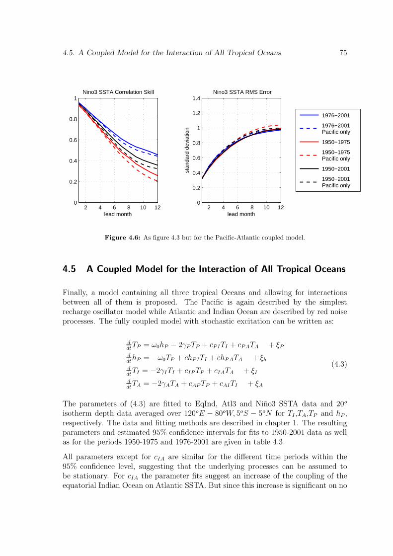
4.5. A Coupled Model for the Interaction of All Tropical Oceans 75
2 4 6 8 10 120
0.2
0.4
0.6
0.8
1
lead month
Nino3 SSTA Correlation Skill
1976−2001
1976−2001 Pacific only
1950−1975
1950−1975 Pacific only
1950−2001
1950−2001 Pacific only
2 4 6 8 10 120
0.2
0.4
0.6
0.8
1
1.2
1.4 Nino3 SSTA RMS Error
lead month
stan
dard
dev
iatio
n
Figure 4.6: As figure 4.3 but for the Pacific-Atlantic coupled model.
4.5 A Coupled Model for the Interaction of All Tropical Oceans
Finally, a model containing all three tropical Oceans and allowing for interactionsbetween all of them is proposed. The Pacific is again described by the simplestrecharge oscillator model while Atlantic and Indian Ocean are described by red noiseprocesses. The fully coupled model with stochastic excitation can be written as:
ddt
TP = ω0hP − 2γPTP + cPITI + cPATA + ξP
ddt
hP = −ω0TP + chPITI + chPATA + ξh
ddt
TI = −2γITI + cIP TP + cIATA + ξI
ddt
TA = −2γATA + cAPTP + cAITI + ξA
(4.3)
The parameters of (4.3) are fitted to EqInd, Atl3 and Nino3 SSTA data and 20o
isotherm depth data averaged over 120oE − 80oW, 5oS − 5oN for TI ,TA,TP and hP ,respectively. The data and fitting methods are described in chapter 1. The resultingparameters and estimated 95% confidence intervals for fits to 1950-2001 data as wellas for the periods 1950-1975 and 1976-2001 are given in table 4.3.
All parameters except for cIA are similar for the different time periods within the95% confidence level, suggesting that the underlying processes can be assumed tobe stationary. For cIA the parameter fits suggest an increase of the coupling of theequatorial Indian Ocean on Atlantic SSTA. But since this increase is significant on no
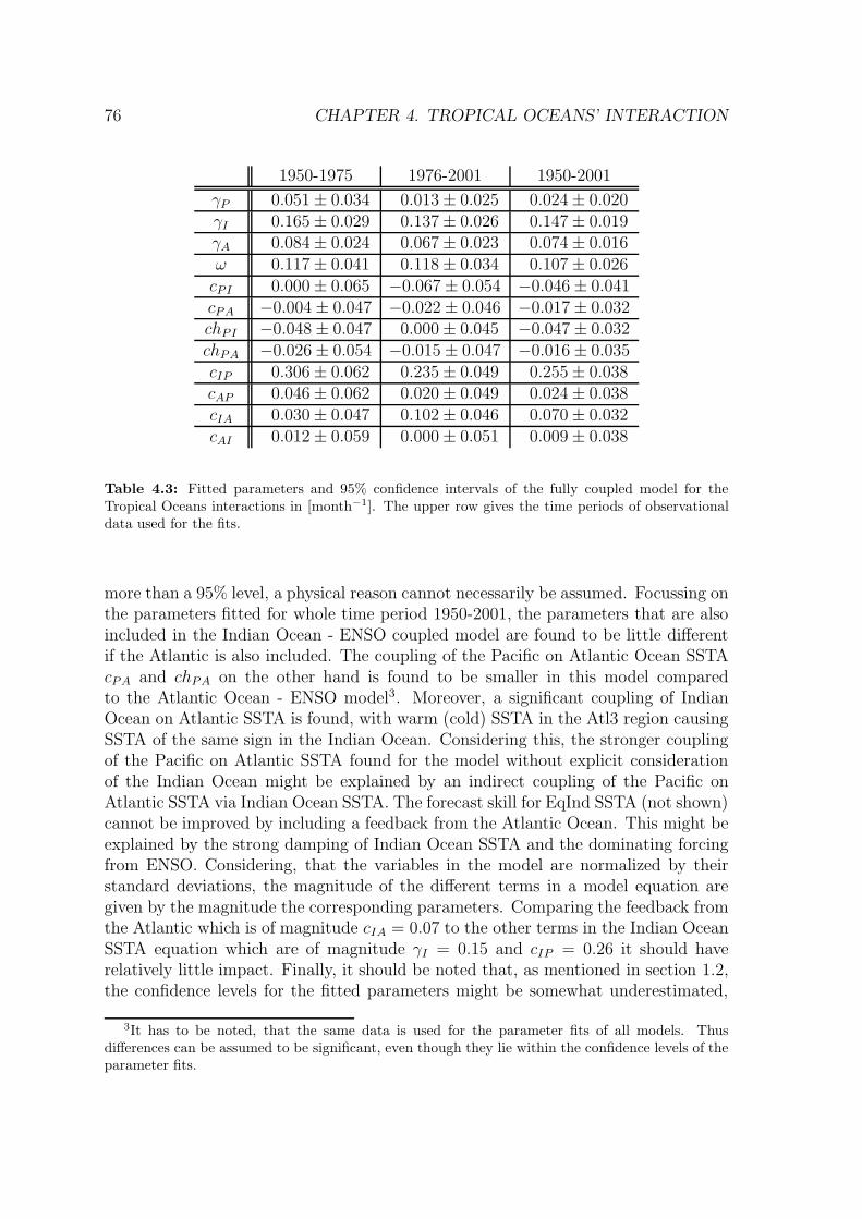
76 CHAPTER 4. TROPICAL OCEANS’ INTERACTION
1950-1975 1976-2001 1950-2001
γP 0.051 ± 0.034 0.013 ± 0.025 0.024 ± 0.020γI 0.165 ± 0.029 0.137 ± 0.026 0.147 ± 0.019γA 0.084 ± 0.024 0.067 ± 0.023 0.074 ± 0.016ω 0.117 ± 0.041 0.118 ± 0.034 0.107 ± 0.026
cPI 0.000 ± 0.065 −0.067 ± 0.054 −0.046 ± 0.041cPA −0.004 ± 0.047 −0.022 ± 0.046 −0.017 ± 0.032chPI −0.048 ± 0.047 0.000 ± 0.045 −0.047 ± 0.032chPA −0.026 ± 0.054 −0.015 ± 0.047 −0.016 ± 0.035cIP 0.306 ± 0.062 0.235 ± 0.049 0.255 ± 0.038cAP 0.046 ± 0.062 0.020 ± 0.049 0.024 ± 0.038cIA 0.030 ± 0.047 0.102 ± 0.046 0.070 ± 0.032cAI 0.012 ± 0.059 0.000 ± 0.051 0.009 ± 0.038
Table 4.3: Fitted parameters and 95% confidence intervals of the fully coupled model for theTropical Oceans interactions in [month−1]. The upper row gives the time periods of observationaldata used for the fits.
more than a 95% level, a physical reason cannot necessarily be assumed. Focussing onthe parameters fitted for whole time period 1950-2001, the parameters that are alsoincluded in the Indian Ocean - ENSO coupled model are found to be little differentif the Atlantic is also included. The coupling of the Pacific on Atlantic Ocean SSTAcPA and chPA on the other hand is found to be smaller in this model comparedto the Atlantic Ocean - ENSO model3. Moreover, a significant coupling of IndianOcean on Atlantic SSTA is found, with warm (cold) SSTA in the Atl3 region causingSSTA of the same sign in the Indian Ocean. Considering this, the stronger couplingof the Pacific on Atlantic SSTA found for the model without explicit considerationof the Indian Ocean might be explained by an indirect coupling of the Pacific onAtlantic SSTA via Indian Ocean SSTA. The forecast skill for EqInd SSTA (not shown)cannot be improved by including a feedback from the Atlantic Ocean. This might beexplained by the strong damping of Indian Ocean SSTA and the dominating forcingfrom ENSO. Considering, that the variables in the model are normalized by theirstandard deviations, the magnitude of the different terms in a model equation aregiven by the magnitude the corresponding parameters. Comparing the feedback fromthe Atlantic which is of magnitude cIA = 0.07 to the other terms in the Indian OceanSSTA equation which are of magnitude γI = 0.15 and cIP = 0.26 it should haverelatively little impact. Finally, it should be noted that, as mentioned in section 1.2,the confidence levels for the fitted parameters might be somewhat underestimated,
3It has to be noted, that the same data is used for the parameter fits of all models. Thusdifferences can be assumed to be significant, even though they lie within the confidence levels of theparameter fits.
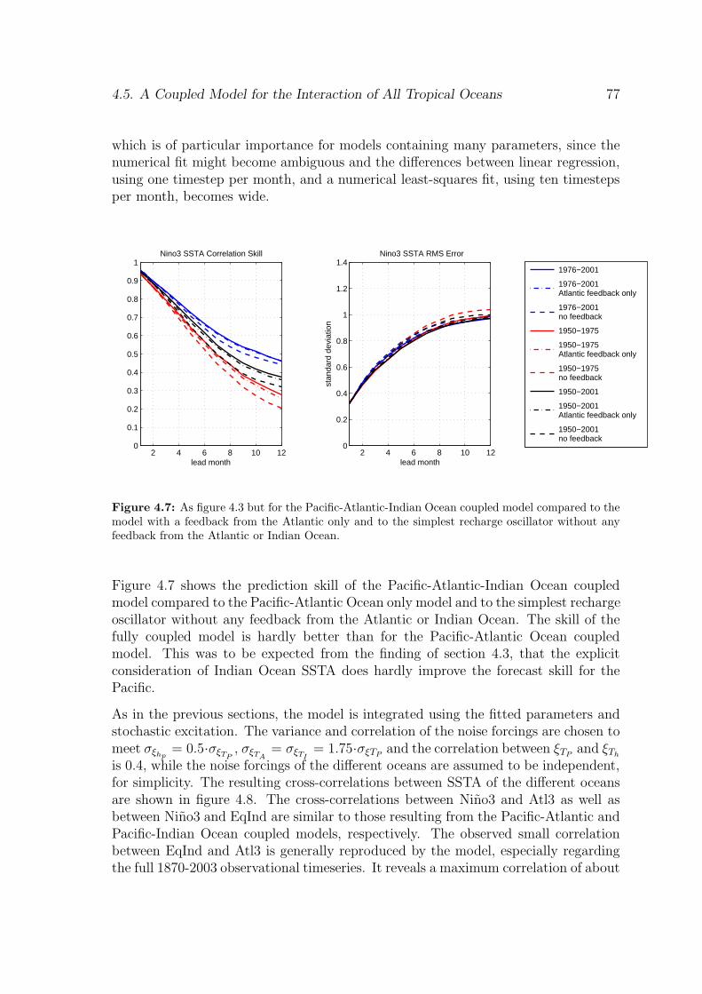
4.5. A Coupled Model for the Interaction of All Tropical Oceans 77
which is of particular importance for models containing many parameters, since thenumerical fit might become ambiguous and the differences between linear regression,using one timestep per month, and a numerical least-squares fit, using ten timestepsper month, becomes wide.
2 4 6 8 10 120
0.1
0.2
0.3
0.4
0.5
0.6
0.7
0.8
0.9
1
lead month
Nino3 SSTA Correlation Skill
1976−2001
1976−2001 Atlantic feedback only
1976−2001 no feedback
1950−1975
1950−1975 Atlantic feedback only
1950−1975 no feedback
1950−2001
1950−2001 Atlantic feedback only
1950−2001 no feedback
2 4 6 8 10 120
0.2
0.4
0.6
0.8
1
1.2
1.4 Nino3 SSTA RMS Error
lead month
stan
dard
dev
iatio
n
Figure 4.7: As figure 4.3 but for the Pacific-Atlantic-Indian Ocean coupled model compared to themodel with a feedback from the Atlantic only and to the simplest recharge oscillator without anyfeedback from the Atlantic or Indian Ocean.
Figure 4.7 shows the prediction skill of the Pacific-Atlantic-Indian Ocean coupledmodel compared to the Pacific-Atlantic Ocean only model and to the simplest rechargeoscillator without any feedback from the Atlantic or Indian Ocean. The skill of thefully coupled model is hardly better than for the Pacific-Atlantic Ocean coupledmodel. This was to be expected from the finding of section 4.3, that the explicitconsideration of Indian Ocean SSTA does hardly improve the forecast skill for thePacific.
As in the previous sections, the model is integrated using the fitted parameters andstochastic excitation. The variance and correlation of the noise forcings are chosen tomeet σξhp
= 0.5·σξTP, σξTA
= σξTI= 1.75·σξTP
and the correlation between ξTPand ξTh
is 0.4, while the noise forcings of the different oceans are assumed to be independent,for simplicity. The resulting cross-correlations between SSTA of the different oceansare shown in figure 4.8. The cross-correlations between Nino3 and Atl3 as well asbetween Nino3 and EqInd are similar to those resulting from the Pacific-Atlantic andPacific-Indian Ocean coupled models, respectively. The observed small correlationbetween EqInd and Atl3 is generally reproduced by the model, especially regardingthe full 1870-2003 observational timeseries. It reveals a maximum correlation of about
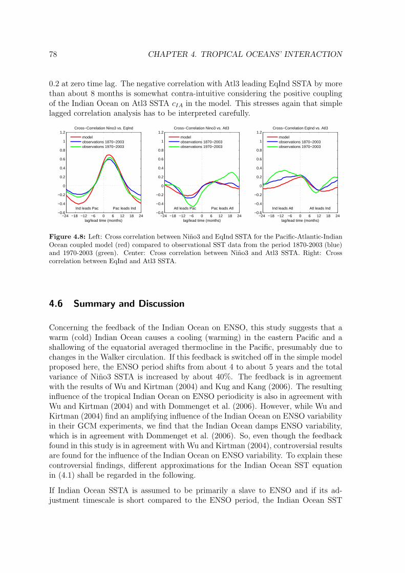
78 CHAPTER 4. TROPICAL OCEANS’ INTERACTION
0.2 at zero time lag. The negative correlation with Atl3 leading EqInd SSTA by morethan about 8 months is somewhat contra-intuitive considering the positive couplingof the Indian Ocean on Atl3 SSTA cIA in the model. This stresses again that simplelagged correlation analysis has to be interpreted carefully.
−24 −18 −12 −6 0 6 12 18 24−0.6
−0.4
−0.2
0
0.2
0.4
0.6
0.8
1
1.2Cross−Correlation Nino3 vs. EqInd
Ind leads Pac Pac leads Ind
lag/lead time (months)
modelobservations 1870−2003observations 1970−2003
−24 −18 −12 −6 0 6 12 18 24−0.6
−0.4
−0.2
0
0.2
0.4
0.6
0.8
1
1.2Cross−Correlation Nino3 vs. Atl3
Atl leads Pac Pac leads Atl
lag/lead time (months)
modelobservations 1870−2003observations 1970−2003
−24 −18 −12 −6 0 6 12 18 24−0.6
−0.4
−0.2
0
0.2
0.4
0.6
0.8
1
1.2Cross−Correlation EqInd vs. Atl3
Ind leads Atl Atl leads Ind
lag/lead time (months)
modelobservations 1870−2003observations 1970−2003
Figure 4.8: Left: Cross correlation between Nino3 and EqInd SSTA for the Pacific-Atlantic-IndianOcean coupled model (red) compared to observational SST data from the period 1870-2003 (blue)and 1970-2003 (green). Center: Cross correlation between Nino3 and Atl3 SSTA. Right: Crosscorrelation between EqInd and Atl3 SSTA.
4.6 Summary and Discussion
Concerning the feedback of the Indian Ocean on ENSO, this study suggests that awarm (cold) Indian Ocean causes a cooling (warming) in the eastern Pacific and ashallowing of the equatorial averaged thermocline in the Pacific, presumably due tochanges in the Walker circulation. If this feedback is switched off in the simple modelproposed here, the ENSO period shifts from about 4 to about 5 years and the totalvariance of Nino3 SSTA is increased by about 40%. The feedback is in agreementwith the results of Wu and Kirtman (2004) and Kug and Kang (2006). The resultinginfluence of the tropical Indian Ocean on ENSO periodicity is also in agreement withWu and Kirtman (2004) and with Dommenget et al. (2006). However, while Wu andKirtman (2004) find an amplifying influence of the Indian Ocean on ENSO variabilityin their GCM experiments, we find that the Indian Ocean damps ENSO variability,which is in agreement with Dommenget et al. (2006). So, even though the feedbackfound in this study is in agreement with Wu and Kirtman (2004), controversial resultsare found for the influence of the Indian Ocean on ENSO variability. To explain thesecontroversial findings, different approximations for the Indian Ocean SST equationin (4.1) shall be regarded in the following.
If Indian Ocean SSTA is assumed to be primarily a slave to ENSO and if its ad-justment timescale is short compared to the ENSO period, the Indian Ocean SST
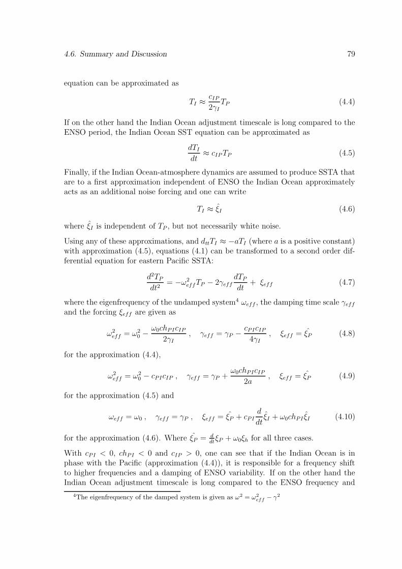
4.6. Summary and Discussion 79
equation can be approximated as
TI ≈ cIP
2γITP (4.4)
If on the other hand the Indian Ocean adjustment timescale is long compared to theENSO period, the Indian Ocean SST equation can be approximated as
dTI
dt≈ cIP TP (4.5)
Finally, if the Indian Ocean-atmosphere dynamics are assumed to produce SSTA thatare to a first approximation independent of ENSO the Indian Ocean approximatelyacts as an additional noise forcing and one can write
TI ≈ ξI (4.6)
where ξI is independent of TP , but not necessarily white noise.
Using any of these approximations, and dttTI ≈ −aTI (where a is a positive constant)with approximation (4.5), equations (4.1) can be transformed to a second order dif-ferential equation for eastern Pacific SSTA:
d2TP
dt2= −ω2
effTP − 2γeffdTP
dt+ ξeff (4.7)
where the eigenfrequency of the undamped system4 ωeff , the damping time scale γeff
and the forcing ξeff are given as
ω2eff = ω2
0 −ω0chPIcIP
2γI
, γeff = γP − cPIcIP
4γI
, ξeff = ξP (4.8)
for the approximation (4.4),
ω2eff = ω2
0 − cPIcIP , γeff = γP +ω0chPIcIP
2a, ξeff = ξP (4.9)
for the approximation (4.5) and
ωeff = ω0 , γeff = γP , ξeff = ξP + cPId
dtξI + ω0chPI ξI (4.10)
for the approximation (4.6). Where ξP = ddt
ξP + ω0ξh for all three cases.
With cPI < 0, chPI < 0 and cIP > 0, one can see that if the Indian Ocean is inphase with the Pacific (approximation (4.4)), it is responsible for a frequency shiftto higher frequencies and a damping of ENSO variability. If on the other hand theIndian Ocean adjustment timescale is long compared to the ENSO frequency and
4The eigenfrequency of the damped system is given as ω2 = ω2eff − γ2
80 CHAPTER 4. TROPICAL OCEANS’ INTERACTION
therefore Indian Ocean SSTA lags Nino3 SSTA by 90o (approximation (4.5)), theIndian Ocean would still be responsible for an increased ENSO frequency but fora reduced damping and therefore increased ENSO variability. Finally, independentIndian Ocean variability (approximation (4.6)) acts as an additional forcing on thePacific and will therefore also increase Pacific Ocean variability, without having aninfluence on the ENSO period.
Observations show a high correlation of Indian Ocean SSTA with Nino3 SSTA witha phase lag that is very small compared to the ENSO frequency. This indicates thatapproximation (4.4) is justified. Therefore, increased ENSO variability and a longerENSO period is found if the Indian Ocean is decoupled.
In the GCM used by Wu and Kirtman (2004) on the other hand, the simulated ENSOhas a peak frequency of about 2.3 years and from their table 2, it can be deferredthat the correlation between Indian Ocean SSTA and Pacific SSTA is smaller thanin observations. This probably makes the approximations (4.5) or (4.6) fit betterto Indian Ocean-ENSO interactions in the GCM. Both approximations lead to lessENSO varibility if the Indian Ocean is decoupled.
Even though it was shown that the Indian Ocean has a considerable influence on theENSO cycle, the forecast skill for Nino3 SSTA of the simple models used here couldhardly be improved by explicitly including the Indian Ocean feedback. This can beexplained by the fact that, at least in this model, Indian Ocean SSTA predictabilityis primarily limited to the SSTA caused by ENSO. The feedback of ENSO-inducedIndian Ocean SSTA back on ENSO, however, is implicitly included if the uncoupledrecharge oscillator is fitted to Pacific data. This can also be seen considering ap-proximation (4.4) which shows that the major effect of the Indian Ocean on ENSOis a shift of ENSO frequency and a strengthening of the damping. This is implicitlycovered if the recharge oscillator model without an Indian Ocean feedback is fittedto Pacific data only.
The coupling of equatorial Atlantic SSTA on ENSO is found to be much weakerthan the coupling of the Indian Ocean on ENSO. However, a significant interactionis found, with an El Nino (La Nina) event causing a warming (cooling) in the Atl3region. Also a feedback from the equatorial Atlantic on ENSO is found with a warm(cold) Atlantic causing a cooling (warming) in the Nino3 region and a shallowing(deepening) of the equatorial averaged thermocline in the Pacific, which is similarto the feedback of the Indian Ocean on ENSO. However, the ENSO cycle is hardlyinfluenced by this feedback. Solely a small reduction of Nino3 SSTA variabilityby about 6% is found if the Atlantic Ocean feedback is switched off in the simplemodel. This is in disagreement with the CGCM results of Dommenget et al. (2006),finding a considerable frequency shift to longer periods if the tropical Atlantic isdecoupled, analog to the effect of the Indian Ocean feedback. These results can againbe explained considering the approximations (4.4) to(4.6). Since in observational dataa very weak coupling of the equatorial Atlantic on Nino3 SSTA is found, compared

4.6. Summary and Discussion 81
to the coupling of the equatorial Indian Ocean on ENSO, the observed situation iswell described by approximation (4.6). As shown by equation (4.10) the Atlanticdoes therefore not influence the eigenfrequency and damping of ENSO. However, thefeedback from the Atlantic is responsible for an additional forcing, which increasesENSO variability. This increase is only weak, since the feedback from the Atlantic onENSO is small. This slight additional noise forcing from the Atlantic is in agreementwith the slightly reduced variance that is found if the Atlantic Ocean feedback isswitched off. In the CGCM used by Dommenget et al. (2006) on the other hand,the equatorial Atlantic responds to Nino3 SSTA quite similar as the Indian Ocean,with a maximum correlation of about 0.7 with Nino3 SSTA leading Atlantic SSTA byabout three months. This justifies approximation (4.4) which explains the frequencyshift to longer periods (see equation (4.8)), assuming that a negative feedback onPacific thermocline depth (chPA < 0), as found in the observations, also exists in theCGCM.
Even though the feedback from the Atlantic Ocean on ENSO is found to be weakerthan the Indian Ocean feedback on ENSO, the forecast skill for Nino3 SSTA of thesimple models used here could be improved somewhat because Atlantic SSTA itselfis more independent from ENSO than Indian Ocean SSTA and might therefore be amore usefull additional predictor.
Finally, a parameter fit of a model containing the Pacific, Atlantic and Indian Oceansto observational data suggests an influence of eastern equatorial Atlantic on equatorialIndian Ocean SSTA. Further, the direct feedback of the Atlantic on ENSO is foundto be smaller than in the model not considering the Indian Ocean, suggesting thatpart of this feedback might be indirect via the Indian Ocean. However, due to thehigh number of parameters in this model, this results have to be handled with care.
Generally, more research addressing the mechanisms of the interactions between thetropical oceans is necessary to support and explain the results of this study.
Appendix A
Eigenvalues of Differential Equations
A linear homogeneous ordinary differential equation (ODE) with constant coefficientsbe given as
y(n)(x) =
n−1∑
k=0
aky(k)(x) (A.1)
with y : R → C, ak ∈ C and y(k) denoting the k’th derivative.
Defining yk := y(k−1) for k = 1..n this can be transformed to a system of first orderODEs
y′(x) = Ay(x) with y : R → Cn and A ∈ C
n × Cn (A.2)
It is therefore apparent that every system of ODEs of the form (A.1) can as well betransformed to a system of first order ODEs of the form (A.2).
It can easily be verified that for all eigenvalues λi and corresponding eigenvectors vi
of A, solutions of (A.2) are given by
y(t) = vi exp(λix) . (A.3)
In climate sciences λi and vi are thus commonly referred to as eigenvalues and eigen-vectors or eigenmodes of the differential equation (A.2).
If A is diagonalizable, the solutions (A.3) represent a fundamental system, whichmeans that the solutions constitute a base for the solution space. If this is not thecase, additional solutions can be found which becomes a little more complicated.However, since this does not happen to be the case in the examples of this study, itis not discussed in further detail here.
82

APPENDIX A. Eigenvalues of Differential Equations 83
It should be added that, after discretizing in space, linear homogeneous systems ofpartial differential equations, such as linear reduced gravity models, can as well betransformed to ODEs of the form A.2. The eigenmodes then correspond to spatialpatterns of the variables contained in the model.
Appendix B
A Correction to Jin (1997)
Jin (1997) proposes estimates for the parameters of the recharge oscillator modelgiven by equation (2.8). The parameter γ is chosen ”to give an SST change rate of1.5oC over 2 months (which is the upwelling timescale) per 10 m of thermocline depthanomaly over the eastern Pacific.” This means γ = 0.075 K
m month. The parameters
are nondimensionalized by scales of [h]=150 m, [T ]=7.5 K and [t]=2 months. Thecorresponding nondimensional value of γ would be γ=3. Though, for the followingdiscussion Jin (1997) uses the nondimensional value γ=0.75. Using γ = 3 withoutchanging any other parameters would alter the discussion dramatically. In the eigen-values of the system, however, γ occurs only in a product with the air sea couplingparameter b = µ b0, which is varied for his discussion via the so-called relative cou-pling coefficient µ. So a big part of the discussion would be unaltered if the tuningparameter was chosen by a factor 4 smaller. The high end estimation of b0, on theother hand is meant to be physically motivated as well.
Concluding, even though the qualitative relevance of the paper is unaltered by thismistake, the quantitative results have to be handled with care.
84
Appendix C
The Power Spectral Density of a RandomProcess Continuous in Time
In climate science one usually only deals with discrete time series. However fortheoretical studies it sometimes interesting to calculate spectra of random processeswhich are continuous in time. The aim is to find the power spectral density of thevariables determined by a linear model of the following form
dxk(t)
dt=
N∑
l=1
aklxl(t) + ξk(t) , k = 1..N (C.1)
with real coefficients akl and white noise forcing ξ(t) . Jin (1997) defines the powerspectral density of such a process as the ensemble mean of the squared Fourier trans-form of the time series:
⟨
|xk(ω)|2⟩
where xk(ω) =
∫
∞
−∞
xk(t) exp(−iωt)dt (C.2)
and 〈〉 denotes the ensemble mean. However, the Fourier transform xk(ω) is welldefined only if
∫
∞
−∞|xk(t)| dt < ∞ which is generally not the case here. Indeed, the
integral in (C.2) would diverge for all processes considered in this study.
Instead, defining
xTk (t) =
xk(t) for − T2
< t < T2
0 else, (C.3)
the power spectral density can be defined as:
85
86 APPENDIX C. The spectrum of a Continuous Random Process
Pxx(ω) = limT→∞
⟨
∣
∣xT (ω)∣
∣
2⟩
T
(C.4)
with
xT (ω) =
∫
T2
−T2
x(t) exp(−iωt)dt =
∫
∞
−∞
xT (t) exp(−iωt)dt . (C.5)
According to the Wiener-Khinchin Theorem as proven in Couch (2001) this definitionof the spectrum is equal to the Fourier transform of the auto-correlation function.
Defining ξTk analog to xT
k and using (C.1) we get:
dxTk (t)
dt=
N∑
l=1
aklxTl (t) + ξT
k (t) , k = 1, ..N ∀ t : |t| 6= T2
. (C.6)
With xTk (t) = 1
2π
∫
∞
−∞xT
k (ω) exp(iωt)dω1 one obtains
∫
∞
−∞
iωxTk exp(iωt)dω =
∫
∞
−∞
(
N∑
l=1
aklxTl + ξT
k
)
exp(iωt)dω , k = 1, ..N . (C.7)
This is true if and only if
iωxTk =
N∑
l=1
aklxTl + ξT
k , k = 1, ..N . (C.8)
This can be solved to get
xTk (ω) =
N∑
l=1
ckl(ω)ξTl (ω) , k = 1, ..N (C.9)
with complex functions ckl(ω) . Using this result one can calculate the spectra bymultiplying (C.9) with its complex conjugate dividing by T and taking the ensemblemean and the limit t → ∞ .
1Strictly speaking, this as well as the following equalities have to be understood between elementsof the L1 space, which means, that functions are identified if they are equal outside of a set of measure0.
APPENDIX C. The spectrum of a Continuous Random Process 87
With the cross-spectral density defined similar to the power spectral density as Pxy =
limT→∞
(
〈xT yT∗〉T
)
the power spectral densities are given as
Pxkxk=
N∑
l=l
N∑
m=1
cklckmPξlξm, k = 1, ..N . (C.10)
Thus the spectra can be written as linear combinations of the spectra and crossspectra of the noise forcings.
Note, that a white noise process continuous in time would always have infinite vari-ance, since it has a constant power spectral density by definition and the total varianceis given by the integral over the power spectrum. Any physically reasonable processis ”white” only up to a certain frequency. But, since the high frequency end of thespectra examined in this study is generally damped proportional to 1
ω2 , we are onlyinterested in the power spectral densities of the noise forcings in the low frequencyrange which are assumed to be constant.
List of Figures
2.1 Parameter regimes of the damped harmonic oscillator. . . . . . . . . . 18
2.2 Forecast skill of the delayed action oscillator. . . . . . . . . . . . . . . 20
2.3 Spectra and frequency distribution of the linear delayed action oscillator. 22
2.4 Parameters of the recharge oscillator. . . . . . . . . . . . . . . . . . . 26
2.5 Forecast skill of the recharge oscillator. . . . . . . . . . . . . . . . . . 27
2.6 Spectra and frequency distribution of the recharge oscillator. . . . . . 29
2.7 Cross correlation between Nino3 SSTA and equatorial Pacific thermo-cline depth. . . . . . . . . . . . . . . . . . . . . . . . . . . . . . . . . 30
2.8 Forecast skill of the linear delayed recharge oscillator. . . . . . . . . . 34
2.9 Cross-correlation of Nino3 SST and Nino3 thermocline depth. . . . . 35
2.10 Spectra and frequency distribution of the linear delayed recharge os-cillator. . . . . . . . . . . . . . . . . . . . . . . . . . . . . . . . . . . 36
2.11 Schematic temperature section through the equatorial Pacific. . . . . 38
2.12 Frequency distribution for Nino3 SSTA. . . . . . . . . . . . . . . . . . 40
2.13 Seasonality of the parameters of the Pacific recharge oscillator. . . . . 41
2.14 Eigenvalues of the recharge oscillator for the Pacific. . . . . . . . . . . 42
2.15 Forecast skill of the recharge oscillator model with seasonal dependentparameters for the Pacific. . . . . . . . . . . . . . . . . . . . . . . . . 43
2.16 Seasonal dependence of forecast skill of the recharge oscillator model. 44
2.17 Spectra and SSTA frequency distribution of the recharge oscillatorwith seasonal dependent parameters. . . . . . . . . . . . . . . . . . . 45
2.18 Seasonal dependence of standard deviation of Nino3 SST for the rechargeoscillator. . . . . . . . . . . . . . . . . . . . . . . . . . . . . . . . . . 46
88
LIST OF FIGURES 89
2.19 Seasonal dependence of Nino3 SSTA auto-correlation and cross-correlationbetween SSTA and equatorial thermocline depth for the recharge os-cillator. . . . . . . . . . . . . . . . . . . . . . . . . . . . . . . . . . . 47
2.20 Forecast skill of the recharge oscillator compared to an hybrid coupledmodel. . . . . . . . . . . . . . . . . . . . . . . . . . . . . . . . . . . . 48
2.21 Seasonality of the parameters of the simplest recharge oscillator model. 49
2.22 Seasonal dependence of standard deviation of Nino3 SSTA for the sim-plest recharge oscillator model. . . . . . . . . . . . . . . . . . . . . . 50
2.23 Seasonal dependence of Nino3 SSTA auto-correlation and cross-correlationbetween SSTA and equatorial thermocline depth for the simplest rechargeoscillator. . . . . . . . . . . . . . . . . . . . . . . . . . . . . . . . . . 51
3.1 Seasonal cycle of the parameters of the recharge oscillator for the At-lantic. . . . . . . . . . . . . . . . . . . . . . . . . . . . . . . . . . . . 55
3.2 Eigenvalues of the recharge oscillator for the Atlantic. . . . . . . . . . 56
3.3 Cross correlation between equatorial Atlantic thermocline depth anoma-lies and Atl3 SSTA. . . . . . . . . . . . . . . . . . . . . . . . . . . . . 57
3.4 Spectrum of Atl3 SSTA. . . . . . . . . . . . . . . . . . . . . . . . . . 58
3.5 Forecast skill for Atl3 SSTA. . . . . . . . . . . . . . . . . . . . . . . . 59
3.6 Seasonal cycle of the parameters of the recharge oscillator for the In-dian Ocean. . . . . . . . . . . . . . . . . . . . . . . . . . . . . . . . . 60
3.7 Eigenvalues of the recharge oscillator for the Indian Ocean. . . . . . . 61
3.8 Indian Ocean DMI spectrum. . . . . . . . . . . . . . . . . . . . . . . 62
3.9 Cross correlation between equatorial Indian Ocean thermocline depthanomalies and DMI. . . . . . . . . . . . . . . . . . . . . . . . . . . . 63
3.10 Forecast skill for the Indian Ocean. . . . . . . . . . . . . . . . . . . . 64
3.11 Parameter regimes of Pacific, Atlantic and Indian Ocean . . . . . . . 64
4.1 Cross correlation between Nino3 and equatorial Indian Ocean SSTA. 69
4.2 SSTA spectrum of the Pacific-Indian Ocean coupled model. . . . . . . 70
4.3 Forecast skill of the Pacific-Indian Ocean coupled model. . . . . . . . 71
4.4 Cross correlation between Nino3 and Atl3 SSTA. . . . . . . . . . . . 73

90 LIST OF FIGURES
4.5 SSTA spectrum of the Pacific-Atlantic coupled model. . . . . . . . . . 74
4.6 Forecast skill of the Pacific-Atlantic coupled model. . . . . . . . . . . 75
4.7 Forecast skill of the Pacific-Atlantic-Indian Ocean coupled model. . . 77
4.8 Cross correlations between Nino3, EqInd and Atl3 SSTA. . . . . . . . 78
List of Tables
1.1 Parameters used for the construction of an artificial data set, units aremonth−1. . . . . . . . . . . . . . . . . . . . . . . . . . . . . . . . . . . 11
1.2 Parameters and confidence intervals resulting from the numerical fitand the linear regression. . . . . . . . . . . . . . . . . . . . . . . . . . 12
2.1 Parameters of the linear delayed action oscillator. . . . . . . . . . . . 19
2.2 Parameters of the recharge oscillator model for the Pacific. . . . . . . 25
2.3 Parameters of the simplest recharge oscillator for the Pacific. . . . . . 31
2.4 Parameters of the linear delayed recharge oscillator model for the Pacific. 33
2.5 Parameters of the nonlinear delayed recharge oscillator model for thePacific . . . . . . . . . . . . . . . . . . . . . . . . . . . . . . . . . . . 39
4.1 Parameters of the Pacific-Indian Ocean coupled model. . . . . . . . . 68
4.2 Parameters of the Pacific-Atlantic Ocean coupled model. . . . . . . . 72
4.3 Parameters of the fully coupled model for the Tropical Oceans inter-actions. . . . . . . . . . . . . . . . . . . . . . . . . . . . . . . . . . . 76
91
Bibliography
Baquero-Bernal, A., M. Latif, and S. Legutke, 2002: On dipolelike variability of seasurface temperature in the tropical Indian Ocean. J. Climate, 15 (11), 1358–1368.
Battisti, D. S. and A. C. Hirst, 1989: Interannual variability in a tropical atmosphere-ocean model: influence of the basic state, ocean geometry and nonlinearity. J.
Atmos. Sci., 46 (12), 1687–1712.
Behera, S. K., S. A. Raoa, H. N. Saji, and T. Yamagata, 2003: Comments on “Acautionary note on the interpretation of EOFs”. J. Climate, 16, 1087–1093.
Bjerknes, J., 1964: Atlantic Air-Sea Interaction. Adv. Geophys., 10, 1–82.
Burgers, G., F.-F. Jin, and G. J. van Oldenborgh, 2005: The simplest ENSO rechargeoscillator. Geophys. Res. Lett., 32, L13 706, doi:10.1029/2005GL022951.
Chang, P., T. Yamagata, P. Schopf, S. K. Behera, J. Carton, W. S. Keesler, G. Mey-ers, T. Qu, F. Schott, S. Shetye, and S.-P. Xie, 2006: Climate fluctuations oftropical coupled systems - The role of ocean dynamics. J. Climate, 19 (20), 5122–5174.
Couch, L. W., 2001: Digital and Analog Communications Systems. 6th ed., PrenticeHall.
Dommenget, D. and M. Latif, 2002: A cautionary note on the interpretation of EOFs.J. Climate, 15, 216–225.
———, 2003: Reply. J. Climate, 16, 1094–1097.
Dommenget, D., V. Semenov, and M. Latif, 2006: Impacts of the tropical In-dian and Atlantic Oceans on ENSO. Geophys. Res. Lett., 33, L11 701, doi:10.1029/2006GL025871.
Dommenget, D. and D. Stammer, 2004: Assessing ENSO simulations and predictionsusing adjoint ocean state estimation. J. Climate, 17 (22), 4301–4315.
Enfield, D. B. and D. A. Mayer, 1997: Tropical Atlantic sea surface temperaturevariability and its relation to El Nino-Southern Oscillation. J. Geophys. Res., 102,929–945.
92
BIBLIOGRAPHY 93
Hasselmann, K., 1976: Stochastic climate models, Part I, Theory. Tellus, 28, 473.
Huang, B., 2004: Remotely forced variability in the tropical Atlantic ocean. Climate
Dyn., 23, 133–152.
Jin, F., J. Neelin, and M. Ghil, 1996: El Nino Southern Oscillation and the annualcycle: Subharmonic frequency-locking and aperiodicity. Physica D, 98, 442–465.
Jin, F.-F., 1997: An equatorial recharge paradigm for ENSO, Part 1: Conceptualmodel. J. Atmos. Sci., 54, 811–829.
Jin, F.-F., L. Lin, A. Timmermann, and J. Zhao, 2007: Ensemble-mean dynamics ofthe ENSO recharge oscillator under state-dependent stochastic forcing. Geophys.
Res. Lett., 43, L03 807, doi:10.1029/2006GL027372.
Keenlyside, N. S. and M. Latif, 2007: Understanding equatorial Atlantic interannualvariability. J. Climate, 20, 131–142.
Kug, J.-S. and I.-S. Kang, 2006: Interactive feedback between ENSO and the IndianOcean. J. Climate, 19 (9), 1784–1801.
Latif, M. and T. P. Barnett, 1995: Interactions of the tropical oceans. J. Climate, 8,952–964.
Latif, M. and A. Grotzner, 2000: The equatorial Atlantic oscillation and its responseto ENSO. Climate Dyn., 16, 213–218.
Levitus, S., R. Burgett, and T. P. Boyer, 1994: World Ocean Atlas, 1994, Salinity,NOAA Atlas NESDIS 3, Vol. 3. Natl. Oceanogr. Data Cent., Sliver Springs, Md.,111 pp.
Marsland, S., H. Haak, J. Jungclaus, and M. Latif, 2003: The Max-Planck-Instituteglobal ocean/sea ice model with orthogonal curvilinear coordinates. Ocean Model.,91–127.
McPhaden, M., 2003: Tropical Pacific Ocean heat content variations and ENSOpersistence barriers. Geophys. Res. Lett., 30 (9), 1480, doi:10.1029/2003GL016872.
Meinen, C. S. and M. J. McPhaden, 2000: Observations of Warm Water VolumeChanges in the Equatorial Pacific and Their Relationship to El Nino and La Nina.J. Climate, 13, 3551–3559.
Neelin, J. D., D. S. Battisti, A. C. Hirst, F.-F. Jin, Y. Wakata, T. Yamagata, andS. E. Zebiak, 1998: ENSO theory. J. Geophys. Res., 103, 14 261–14 290.
Penland, C. and P. D. Sardeshmukh, 1995: The optimal growth of tropical sea surfaceanomalies. J. Climate, 8 (8), 1999–2024.
94 BIBLIOGRAPHY
Rayner, N. A., D. E. Parker, E. B. Horton, C. K. Folland, L. V. Alexander, D. P.Rowell, E. C. Kent, and A. Kaplan, 2003: Global analyses of sea surface temper-ature, sea ice, and night marine air temperature since the late nineteenth century.J. Geophys. Res., 108 (D14), 4407, doi:10.1029/2002JD002670.
Ruiz-Barradas, A., J. A. Carton, and S. Nigam, 2000: Structure of interannual-to-decadal climate variability in the tropical Atlantic sector. J. Climate, 13, 3285–3297.
Saji, N., B. Goswami, P. Vinayachandran, and T. Yamagata, 1999: A dipole modein the tropical Indian Ocean. Nature, 401 (6751), 360–363.
Saravanan, R. and P. Chang, 2000: Interaction between tropical Atlantic variabilityand El Nino-Southern Oscillation. J. Climate, 13, 2177–2194.
Schopf, P. S. and R. J. Burgman, 2006: A simple mechanism for ENSO residuals andasymmetry. J. Climate, 19 (13), 3167–3179.
Suarez, M. J. and P. S. Schopf, 1988: A delayed action oscillator for ENSO. J. Atmos.
Sci., 45 (21), 3283–3287.
Venzke, S., M. Latif, and A. Villwock, 2000: The coupled GCM Echo-2. Part II:Indian Ocean response to ENSO. J. Climate, 13 (8), 1371–1383.
von Storch, H. and F. W. Zwiers, 1999: Statistical Analysis in Climate Research.Cambridge University Press.
Webster, P., A. Moore, J. Loschnigg, and R. Leben, 1999: Coupled ocean-atmospheredynamics in the Indian Ocean during 1997-98. Nature, 401 (6751), 356–360.
Wu, R. and B. P. Kirtman, 2004: Understanding the impacts of the Indian Ocean onENSO variability in a coupled GCM. J. Climate, 17 (20), 4019–4031.
Xue, Y., A. Leetmaa, and M. Ji, 2000: ENSO prediction with Markov models: Theimpact of sea level. J. Climate, 13 (4), 849–871.
Yu, J.-Y., C. R. Mechoso, J. C. McWilliams, and A. Arakawa, 2002: Impacts ofthe Indian Ocean on the ENSO cycle. Geophys. Res. Lett., 29 (8), 1204, doi:10.1029/2001GL014098.
Zebiak, S. E., 1993: Air-sea interaction in the equatorial Atlantic region. J. Climate,6, 1567–1586.
Zebiak, S. E. and M. A. Cane, 1987: A model El Nino-Southern Oscillation. Mon.
Wea. Rev., 115, 2262–2278.

95
Acknowledgments
First and foremost I would like to thank Dietmar Dommenget who gave me goodadvice and still enough freedom. Thanks as well to Noel Keenlyside and Mojib Latif.
Thanks to Alex for interesting mathematical discussions, to Andi and the other physi-cists in Heidelberg, and to Astrid, Mirjam and Tim for our interdisciplinary coffeebreaks and many other things...
Finally, special thanks to my parents for their support and their trust in me at alltimes.

Erklarung
Hiermit erklare ich, dass ich die vorliegende Diplomarbeit selbstandig verfasst undkeine anderen als die angegebenen Quellen und Hilfsmittel verwendet habe. Ich ver-sichere, dass diese Arbeit noch nicht an anderer Stelle zur Erlangung eines akademis-chen Grades vorgelegen hat.
Kiel, 15. Juni 2007
Malte Jansen