Sikuliaq 2014 UHDAS installation and ADCP evaluation

Dr. Julia M Hummon

University of Hawaii

hummon@hawaii.edu Revision History

08/05/14 draft

09/03/14 final

Table of Contents1 Hardware and software setup.............................................................................................1

1.1 ADCPs...........................................................................................................................11.2 Computer......................................................................................................................2

1.2.1 Serial Feeds........................................................................................................21.2.2 CODAS processing settings ...........................................................................3

2 ADCP Evaluation...................................................................................................................32.1 Biases.............................................................................................................................42.2 Bubbles..........................................................................................................................52.3 Acoustic Interference (other instruments)...............................................................92.4 Sync (K-Sync) triggering...........................................................................................15

3 Recommendations...............................................................................................................183.1 Installation..................................................................................................................183.2 Hardware....................................................................................................................183.3 Operations..................................................................................................................18

1 Hardware and software setup

RV Sikuliaq has two Acoustic Doppler Current Profilers (ADCPs) made by Teledyne RDI. These instruments are used to determine ocean currents beneath the ship. Data acquisition and processing at sea will be performed by the University of Hawaii Data Acquisition System (UHDAS), written and maintained by the University of Hawaii ADCP group. This document describes UHDAS and the installation of the system on Sikuliaq as of Aug 25, 2014.

1.1 ADCPs

The two ADCPs are 75 kH and 150 kHz Ocean Surveyors (OS75 and OS150). The original OS150 was damaged upon delivery, and the original OS75 deck unit was faulty. Both were replaced and passed RDI dockside diagnostic tests in spring 2014.

Initial data from the OS150 showed very poor range. Diagnostic self-tests indicated a problem with 2 beams. Inspection of the transducer cable revealed a bent pin in the connector that attaches to the deck unit. After it was straightened, performance improved to normal. This pin in the OS150 connector is now weak, and care must be used when reseating the connector. It is possible that a new connector would be required if this pin were to break.

1.2 Computer

ADCP data acquisition is performed by a computer purchased by UAF for the purpose. The computer was set up in 2013 with 64-bit Xubuntu 12.04. The operating system was updated (reinstalled) at WHOI in August 2014, with Xubuntu 14.04, prior to the multibeam trials. The computer has hardware RAID and a 2Tb disk capacity. The acquisition software gathers data from the ADCP and other serial feeds through an 8-port serial-USB device. UHDAS logs and timestamps ADCP data, heading (gyro1, gyro2, Seapath), and GPS positions, and writes them to disk. During the processing stage, ADCP beam velocities are transformed into horizontal velocities and referenced to earth prior to automated editing and averaging. The software also populates a website with a variety of plots and links to data and documentation. The website and all of the raw and processed data should be accessible within the ship's network. Some work remains to complete this aspect. A daily email is automatically generated, which contains a snippet of processed data as well as diagnostics related to data acquisition, processing and computer system. The email is sent to shore, where it is monitored by UHDAS personnel, and where figures are generated from the data snippet. Information from the email is available at this web site: http://currents.soest.hawaii.edu/uhdas_fromships.html

1.2.1Serial Feeds

UHDAS uses one process per serial port for data acquisition. The input streams are filtered by message, timestamped, and written to a directory named after the instrument being logged. More than one NMEA string can be acquired from a given serial stream. If the rate of repetition is too high, messages may be subsampled prior to recording (eg. both gyros on Sikuliaq). The file sensor_cfg.py contains settings for serial acquisition, including ports, baud rates, and message strings. (NOTE that indentation must be respected when editing sensor_cfg.py, as it is written in Python). CODAS processing requires position and heading. We try to log all required input types from multiple sources, to allow for reprocessing (in case of gaps or failure in the primary serial feed).

Serial messages logged

Serial (raw) directory

instrument suffix messages serial port/dev/tty/

seapath Seapath 320 sea, gps_sea $GPGGA;$PSXN,20;$PSXN,23; $GPHDT

USB0

cnav C-nav gps $GPGGA USB1gyro1 4913 FOG hdg $HEHDT USB2gyro2 4913 FOG hdg $HEHDT USB3os150 RDI ADCP

(150kHz)raw, log, log.bin (binary adcp data + log files) USB6

os75 RDI ADCP (75kHz)

raw, log, log.bin (binary adcp data + log files) USB7

NOTE: These ports are numbered 0,1,...7 (not 1,2,..8)

1.2.2CODAS processing settings

Settings for heading and position source, and transducer angle are:

heading(reliable)

best position

heading correction(accurate)

transducer angleos75

transducerangle

os150

gyro1 $HEHDT

cnav $GPPGA

seapath $PSXN,20/PSXN,23

45.5 69.8

If necessary, processing of UHDAS data can be redone at a later date using different supporting serial strings. Should there be a problem with the primary data feeds, reprocessing of UHDAS data on Sikuliaq should be able to use appropriate settings chosen from:

instrument position/time reliable heading accurate headingSeapath $GPGGA $PSXN,20;$PSXN,23

CNav $xxGGAgyro1 $HEHDTgyro2 $HEHDT

A scale factor (multiplying measured velocities) is theoretically unnecessary with Ocean Surveyors, but they typically require a multiplier of about 1.003-1.004; preliminary calculations suggested 0.997 for the OS150 and 1.007 for the OS75. Further refinement of these values will occur as we gain experience with the installation.

Additional information about CODAS processing and UHDAS can be found here: http://currents.soest.hawaii.edu/docs/adcp_doc/index.html

Other reports are stored on line at http://currents.soest.hawaii.edu/reports/ship_reports/

2 ADCP Evaluation

UHDAS was run during periods of the multibeam acceptance trials when the EM302 and EM710 were not being tested or calibrated. During these periods tests were performed to determine transducer orientation, to measure effective instrument ranges at different sea conditions and ship speeds, to check for common biases in the data, and to look at interference between acoustic instruments.

To determine the precise orientation of the ADCPs relative to the Seapath 320, bottom track data was accumulated during the transit away from WHOI and while returning to WHOI after the multibeam trials.

Most tests were run with both ADCPs running. Some tests used narrowband mode only, and some used broadband and narrowband mode. In general, they were not synchronized. There were opportunities to compare broadband to narrowband mode (for a given instrument) as well as compare the two instruments with each other. There was sufficient time during the multibeam trials to allow a speed+range test during one transit, as well as multiple mini-surveys of a site at 550m with various combinations of ADCP, EM302, EM710, EK60, and some experimentation using the Kongsburg K-Sync to trigger the devices. Tests took place in 2500m water depth or less, with winds 5-40kts, and varying sea state.

Values determined during ADCP testing:

OS150 OS75

Correlation Magnitude(before cable inspection)

RSSI: 29 20 1 1RSSI: 45 31 0 1

NOTE: “PASSED” --- two beams were weak; why did it say “passed”?

NOTE: RSSI is signal return strength. Expected values 20-40: high values (50-100) may indicate interference (acoustic or electrical); very low (0-5) indicates a problem

Correlation Magnitude

RSSI: 40 24 26 48 RSSI: 22 22 35 23RSSI: 35 30 25 29RSSI: 73 69 71 66

Receive Bandwidth

Expected Bm1 Bm2 Bm3 Bm4 -------- ----- ----- ----- ----- 15500 14978 14864 15343 15165 15500 14915 14878 15271 15193 15500 14872 14920 14922 14670

Expected Bm1 Bm2 Bm3 Bm4 -------- ----- ----- ----- ----- 7750 8121 8017 8100 8035 7750 8052 8045 8072 7995

Wakeup message

Frequency: 153600 HZ Configuration: 4 BEAM, JANUS Transducer Type: ROUND 32x32 Beamformer Rev: A02 or later Beam Angle: 30 DEGREES Beam Pattern: CONVEX Orientation: DOWN CPU Firmware: 23.17 FPGA Version: AA Sensors: TEMP

Frequency: 76800 HZ Configuration: 4 BEAM, JANUS Transducer Type: ROUND 32x32 Beamformer Rev: A02 or later Beam Angle: 30 DEGREES Beam Pattern: CONVEX Orientation: DOWN CPU Firmware: 23.17 FPGA Version: AA Sensors: TEMP SYNCHRO

transducer angle (EA)

69.8 (relative to Seapath) 45.5 (relative to Seapath)

deepest Bottom Track

300m 520m (could be deeper; limited testing opportunity)

deepest Watertrack Range

Broadband (4m bins) 170mNarrowband (8m bins) 300m

Broadband (8m bins) 500mNarrowband (16m bins) 600m

2.1 Biases

During the Sea Trials, ADCP data were collected with both instruments using interleaved

mode (BB and NB pings). Defaults for each instrument and each ping type (and blanking) were the defaults recommended by the manufacturer. Comparisons between ping types and instruments did not suggest that there is any problem with the broadband mode. The OS150NB mode and OS75NB mode differed in the along-track direction, but a small independently-determined scale factor applied to each dataset decreased that difference to only a few cm/s. There was no indication of ringing in either instrument when the default blanking interval was used. Bias in the along-track direction may occur due to bubbles, becoming more obvious as the number of good values decreases. Post-processing algorithms may reduce bias from this source.

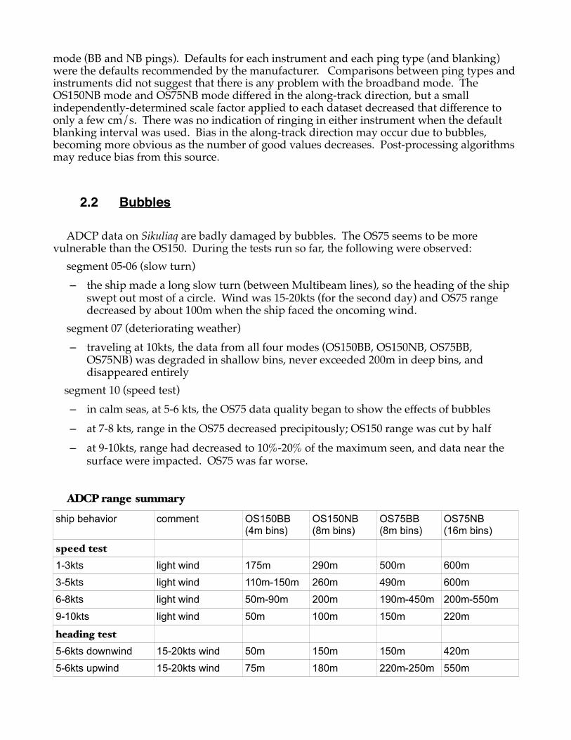
2.2 Bubbles

ADCP data on Sikuliaq are badly damaged by bubbles. The OS75 seems to be more vulnerable than the OS150. During the tests run so far, the following were observed:

segment 05-06 (slow turn)– the ship made a long slow turn (between Multibeam lines), so the heading of the ship

swept out most of a circle. Wind was 15-20kts (for the second day) and OS75 range decreased by about 100m when the ship faced the oncoming wind.

segment 07 (deteriorating weather)– traveling at 10kts, the data from all four modes (OS150BB, OS150NB, OS75BB,

OS75NB) was degraded in shallow bins, never exceeded 200m in deep bins, and disappeared entirely

segment 10 (speed test)– in calm seas, at 5-6 kts, the OS75 data quality began to show the effects of bubbles– at 7-8 kts, range in the OS75 decreased precipitously; OS150 range was cut by half– at 9-10kts, range had decreased to 10%-20% of the maximum seen, and data near the

surface were impacted. OS75 was far worse.

ADCP range summary

ship behavior comment OS150BB (4m bins)

OS150NB (8m bins)

OS75BB (8m bins)

OS75NB (16m bins)

speed test1-3kts light wind 175m 290m 500m 600m3-5kts light wind 110m-150m 260m 490m 600m6-8kts light wind 50m-90m 200m 190m-450m 200m-550m9-10kts light wind 50m 100m 150m 220m

heading test5-6kts downwind 15-20kts wind 50m 150m 150m 420m5-6kts upwind 15-20kts wind 75m 180m 220m-250m 550m

Figure 1: Speed Test: OS150 range is reduced as ship speed increases; OS75 range is slightly reduced until a precipitous loss of range, at about 6.5kts. The actual speed at which the OS75 range drops, will vary with sea state.

Figure 2: Heading test: As the ship rounded a long slow turn, range of each instrument and ping-type was reduced. Impact on OS75 was about 100m reduction of range, even at 5-6kts ship speed. OS150 started with poor range, that was further reduced when the ship headed into the seas.

2.3 Acoustic Interference (other instruments)

Acoustic interference by other sonars was tested by running the OS150 and OS75 simultaneously but unsynchronized, and then watching the additional effect on the ADCP data by turning on other sonars for a period of 10min and alternating [off, on, off, on]. It would have been better to do this test with each ADCP independently, but there was not time. The sonars tested were: EM302, EM710, and the 5 frequencies of the EK60. Qualitative observations are:

– OS150 is not obvious in the OS75 amplitude data– OS75 is very obvious in the OS150 data, and if not edited out, leads to biases in the

averaged product– EK60 has a very short pulse, and the higher frequencies (200kHz, 120kHz) are not

visible in the amplitude of either ADCP. The lowest frequency (18kHz) was also not visible. The 70kHz was visible in amplitude but not velocity, for both ADCPs. The 38kHz was barely visible in the OS150 amplitude and not obvious in the velocity; it was obvious in the OS75 amplitude, but seemed to only affect OS75 broadband velocities. 70kHz EK60 affected the ADCPs similarly to the 38kHz, but apparently did not cause the same damage to the OS75 broadband velocities.

– EM302 was obvious in the amplitudes of both ADCPs, but not obvious in the velocities in either broadband or narrowband mode.

– EM710 was also obvious in the amplitudes of both ADCPs, and was visible in both broadband and narrowband mode of the OS150 velocities. EM710 affected broadband mode badly, but was not apparent in narrowband mode.

– TOPAZ and Knudsen are likely to be obvious in amplitudes, and may affect velocities. – In all cases, as long as the data are asynchronous (free-running, NOT triggered) the

CODAS processing of ADCP data can generally find and edit out the interference from the other instruments.

– These interference tests should be repeated, but with each ADCP running alone. To save time, they could be run with both broadband and narrowband modes enabled.

The following three figures are examples of acoustic interference on ADCP data. They are all laid out with the same scheme:

– upper left: beam 1 backscatter (“RSSI”) (color panel plot)– lower left: “interference mask” created from amplitude spikes (eg. in upper left)– upper center: beam 1 velocity (color panel plot)– lower center: final computed ocean velocity (oriented in ship's forward direction)– upper right: beam velocity plotted versus depth; “bad” values (as determined from the

“interference mask” are plotted in red– lower right: final computed ocean velocity plotted versus depth

Interference from the OS75 is visible in amplitude and velocity in the OS150, as shown above. Interference from the OS150 is barely discernible in the OS75 amplitude and velocity.

Figure 3: OS75 interference is visible in OS150 amplitude (top left) and velocity (bottom left). Masking bad bins based on amplitude (upper right) identifies most of the bad values in velocity (bottom right). A lower threshold in the amplitude spike detection would eliminate more of the remaining bad velocities.

Figure 4: EM710 is visible in amplitude and velocity in the OS75 broadband mode (top left and center panels) Amplitude spikes are used to create a mask (lower left) and account for most outliers in beam velocity (upper right). The final calculated velocity, shown oriented in the ship's forward direction (lower center and right) does not have many outliers.

Quantitative use of EK60 requires calibration of the sonars and probably requires that other sonars be synced or secured. Qualitative use of the EK60 may not require this.

The MAC (Multibeam Advisory Committee) indicated that the OS150 and OS75 do not significantly impact deep multibeam sonar bathymetry mapping (EM302 (or EM122, if there is one)). If science cruise requirements need water-column data, it is up to the science team to decide whether to secure or trigger the ADCPs. The EM710 is impacted by the OS75 and OS150, and mapping with the EM710 will probably require that at least the OS75 (and possibly the OS150) be triggered or secured.

2.4 Sync (K-Sync) triggering

All of these instruments rely on backscattered sound, but use it in different ways. ADCPs

Figure 5: EM710 is visible in amplitude but NOT velocity in the OS75 narrowband mode (top left and center panels) Amplitude spikes are used to create a mask (lower left) and account for only a few points in the beam velocity (upper right). The final calculated velocity, shown oriented in the ship's forward direction (lower center and right) does not have many outliers.

measure the Doppler shift caused by the component of velocity measured along each of the 4 beams. Given typical ocean velocities, this is a small quantity that can be difficult to isolate, particularly from the weak returns at the edge of the instrument's range. Therefore, the measurement is inherently noisy, and many pings (on the order of 50 to 300 in a 5 minute averaging period) are needed to adequately determine ocean velocities.

Since these various sonars can interfere with each other, it is natural to try timing their pings in such a way as to minimize this interference. Sikuliaq has a device (a Kongsberg K-Sync) designed to enable this. Unfortunately this approach can also damage the data. For the ADCPs there are two problems : 1) It reduces the number of pings. Since the Doppler measurement is inherently noisy, reducing the ping rate increases the uncertainty of the results. If the number of pings drops too low, the data become essentially worthless. 2) If there is still interference, synchronized ping timing ensures that the interference is always at the same depth. This means there will be no valid data at all from that depth. Since interference can usually be edited out by the automatic processing, the ADCPs acquired with UHDAS work better with the pseudo-randomly distributed noise from uncoordinated pinging, even if the total amount of interference is greater.

If there is no science mandate otherwise, the ADCPs should not be synchronized to other devices. If there is a scientific need to run the ADCPs and synchronize them with other devices (eg. EK60), proper settings should be used. There was insufficient time during these tests to learn what settings are most appropriate.

Figure 3: KSync test with EM302 in "automatic" mode, allowing it to change ping and pulse rate based on its own estimation of depth. This figure shows the effect on ADCP pingrate as the ship moved from deeper to shallower water. The EM302 pulse impacted the ADCP amplitude and velocities.

3 Recommendations

3.1 Installation

Bubbles badly affect the performance of both ADCPs. Range, quality of pings, and number of pings are all adversely affected. At present, the only way to get full range is to slow the ship. It is strongly recommended that some action be taken to reduce the bubble sweep-down problem under the hull.

3.2 Hardware

Purchase a spare connector for the OS150 transducer cable, because the bent ping is likely to fail in the future. Reterminating the cable is time-consuming and requires good soldering skills, but does not necessarily require an RDI tech to perform the operation.

3.3 Operations

Because both OS150 and OS75 appear to be working, and because NB mode is the deepest, most robust setting, defaults will be set to OS150NB (8m) and OS75NB (16m). There is no problem running either instrument in broadband mode if science on a cruise warrants it. Broadband mode does have higher accuracy (can use smaller bins) but is far more prone to fail in the presence of bubbles or lack of scattering.

When the ship has moved to the Alaska and is likely to have shallow water cruises, it might make sense to have smaller Narrowband bins for shallow water. But we will wait for the ice trials to determine those settings.In the meantime:

(1) Do not synchronize the ADCPs unless the scientific mission requires it(2) Slow the ship (to decrease bubble layer) to improve depth penetration(3) Default settings for OS150: 8-m bins, narrowband mode(4) Default settings for OS75: 16-m bins, narrowband mode