Embed Size (px)
Citation preview

Si-W ECAL Tests en faisceau du
prototype
Cristina Cârloganu
Clermont Ferrand

!"#$%&'(&)*+,*&-./0&1''( Djamel BOUMEDIENE, CALICE collaboration 2312
!"#$%&'()()*+,
#-.('-,'%/%!"#$%!&#
#0)12,%,3,4,5)%/%%'(')*#
6178%.94+3157%/%+,-(./&0%
6178%7'95:39'1)*%/%121-)34)&((%
"(4+90)%/%5-6,-)3-7&8!9-:*0-
6;-<,
"8955,3.%/ =;>1-?6,,=@
#%8178%7'95:39'1)*%093('14,),'%(+)141;,<%=('%Particle Flow =('%>$"%+8*.10.
C Cârloganu, LPNHE, 30.06.08 SiW ECAL : tests en faisceau du prototype
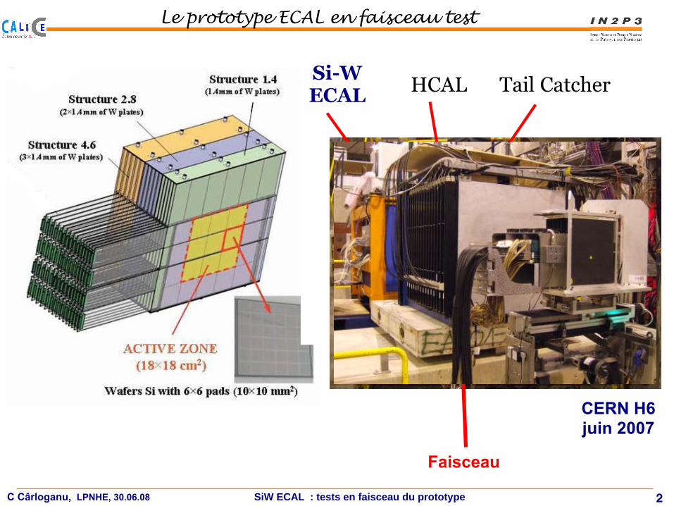
Le prototype ECAL en faisceau test
2
HCAL Tail CatcherSi-W ECAL
CERN H6juin 2007
Faisceau
!"#$%&'(&)*+,*&-./0&1''( Djamel BOUMEDIENE, CALICE collaboration 2312
!"#$%&'()()*+,
#-.('-,'%/%!"#$%!&#
#0)12,%,3,4,5)%/%%'(')*#
6178%.94+3157%/%+,-(./&0%
6178%7'95:39'1)*%/%121-)34)&((%
"(4+90)%/%5-6,-)3-7&8!9-:*0-
6;-<,
"8955,3.%/ =;>1-?6,,=@
#%8178%7'95:39'1)*%093('14,),'%(+)141;,<%=('%Particle Flow =('%>$"%+8*.10.
C Cârloganu, LPNHE, 30.06.08 SiW ECAL : tests en faisceau du prototype
Le prototype ECAL en faisceau test
2
HCAL Tail CatcherSi-W ECAL
CERN H6juin 2007
Faisceau

C Cârloganu, LPNHE, 30.06.08 SiW ECAL : tests en faisceau du prototype
Le prototype ECAL SiW en faisceau test
3
mai 06
aout -sept06
DESY, 24 couches, 6 wafers/couche
CERN, 30 couches, 6 wafers/couche
CERN, 30 couches, 6 wafers/coucheoct 06
CERN, 30 couches, 9 wafers/couchejuillet -aout07

C Cârloganu, LPNHE, 30.06.08 SiW ECAL : tests en faisceau du prototype
Le prototype ECAL SiW en faisceau test
3
mai 06
aout -sept06
DESY, 24 couches, 6 wafers/couche
CERN, 30 couches, 6 wafers/couche
CERN, 30 couches, 6 wafers/coucheoct 06
CERN, 30 couches, 9 wafers/couchejuillet -aout07
e- 1-6 GeV, 5 angles, 3 positions, 8 M triggers
ECAL+AHCAL: pi 30-80 GeV, 3 angles, 1.7 M triggersECAL: e- 10-45 GeV, 4 angles, 8.6 M triggers 30 M muons pour la calibration.
ECAL+AHCAL+TCMT: e+, e-: 3.8 M triggers, 6-45 GeV π+,π-: 22 M triggers, 6-80 GeV 40 M muons pour la calibration.
ECAL, HCAL, TCMT: 4 angles, 12 positions e+, e-,π+,π-: 200 M triggers, 6-80 GeV
!"#$%
&'()*+),
-.)*&&'
/-012324
)5-67-8419
()%:;#
'
Summary of the data taken
Summary of the data taken
5239)4<)=2>?@)A
)B&)?CD978
!EF,
)979<8>)
G)*HF)IC
)J41)!K
%L)MN.
>2O>)1P<
>
!Q)+&
),)G)R)IC)J4
1)SP4<
)O-6201-
824<)1P<
>
!"#"$%&
'()*+,
-.%+/(
)&'()*+,
0('%1&/)
(23
! .24*/1&)"5$
! .24*/1

C Cârloganu, LPNHE, 30.06.08 SiW ECAL : tests en faisceau du prototype
Management des données
4
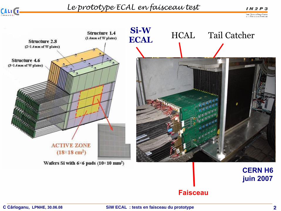
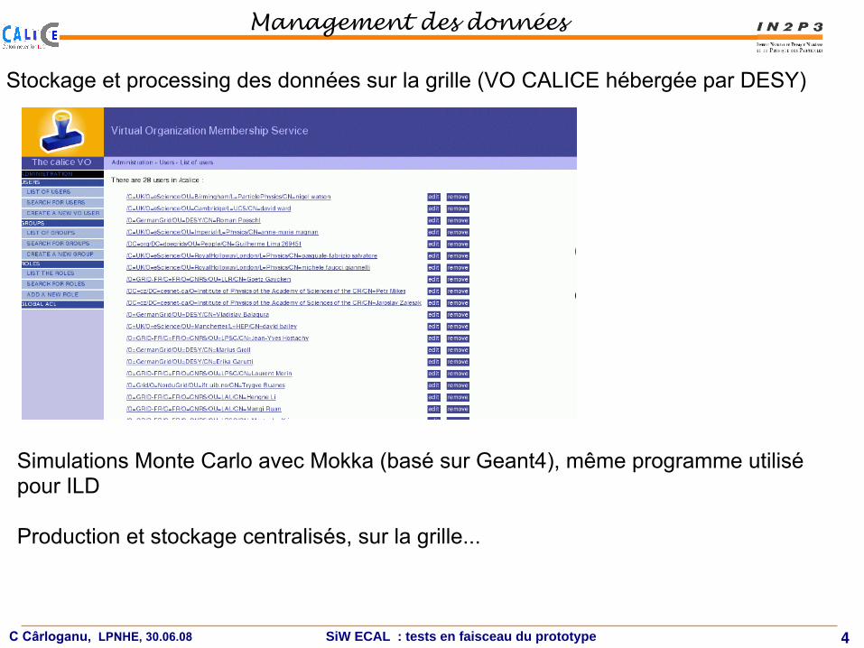
Stockage et processing des données sur la grille (VO CALICE hébergée par DESY)

C Cârloganu, LPNHE, 30.06.08 SiW ECAL : tests en faisceau du prototype
Management des données
4
!!!"#$%&'%()*+,-%.,/0%1&&'
!"#$%&'()*+$,'-*.&/*(&0.$1$20$3*+&3#
40/(#5$67$89:;<=*-#$>0'$'#-&/('*(&0.$&/$"((?/<@@-'&5120A/B5#/7B5#<CDDE@20A/@3*+&3#
VO Manager: R.P./ LAL, Deputy: A. Gellrich/ DESY
FE$G#A6#'/$$$*.5$30).(&.-$BB
C
8*(*$A*.*-#A#.($*.5$?'03#//&.-$67$)/&.-$("#$-'&5$
Stockage et processing des données sur la grille (VO CALICE hébergée par DESY)
Simulations Monte Carlo avec Mokka (basé sur Geant4), même programme utilisé pour ILD
Production et stockage centralisés, sur la grille...

C Cârloganu, LPNHE, 30.06.08 SiW ECAL : tests en faisceau du prototype
Le prototype ECAL SiW en faisceau test
5
Excellent fonctionnement du détecteur - très grande stabilité de l’électronique (monitorée en temps réel et calibrée avec des MIPs)
Sur l’ensemble des voies:
• 98,6% des voies fonctionnelles • bruit moyen par voie : 0.13 MIPs • dispersion du bruit voie à voie 0.012 MIPs
C Cârloganu, LPNHE, 30.06.08 SiW ECAL : tests en faisceau du prototype
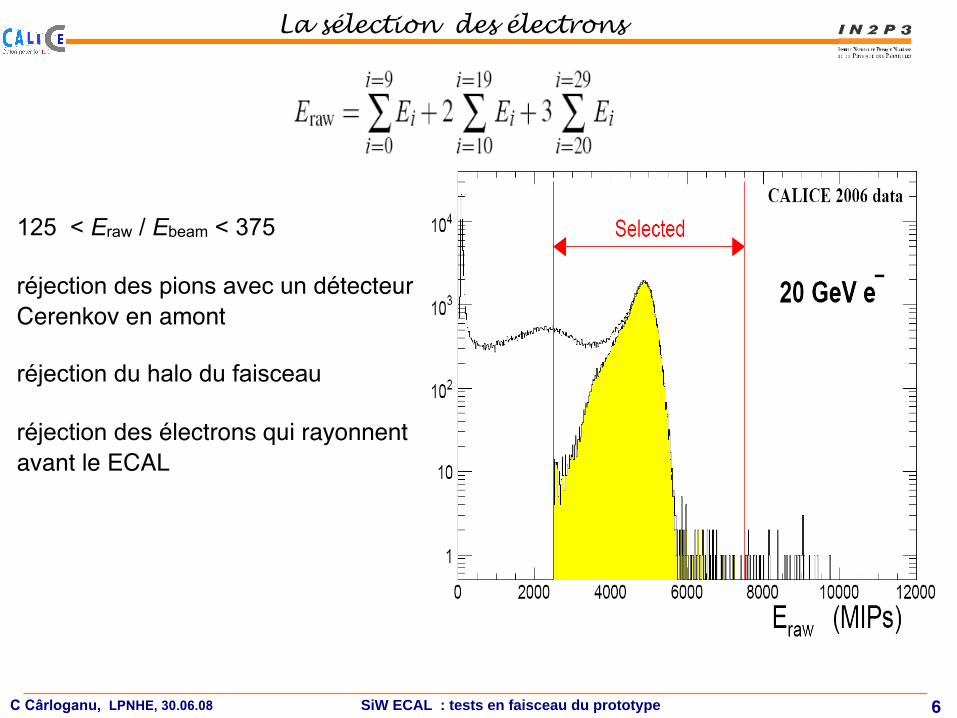
La sélection des électrons
6
125 < Eraw / Ebeam < 375
réjection des pions avec un détecteur Cerenkov en amont
réjection du halo du faisceau
réjection des électrons qui rayonnent avant le ECAL

impinging on the calorimeter at normal incidence. Here the mean value of Eraw(Eq. 5.1) is plottedas a function of the shower barycentre (x, y), defined as :
(x, y) =!i
(Eixi,Eiyi)/!i
Ei
The sums run over all hit cells in the calorimeter. Dips in response corresponding to the guardring positions are clearly visible. According to Figure 6, which shows the mean value of E raw as afunction of the shower barycentre for 20 GeV electrons, the energy loss is about 15 % when tracksimpinge in the centre of the x gaps and about 20 % in the case of the y gap.
CALICE 2006 data
!50 !40 !30 !20 !10 0 10 20 30 40
Y (
mm
)
!30
!20
!10
10
20
0
2
4
6
8
10
12
14
16
X (mm)
30
0
!40
Figure 4. Mean values of Eraw for a 15 GeV e− beam as function of the barycentre coordinates.
In order to recover this loss and to have a more uniform calorimeter response, a simple methodwas investigated. The ECAL energy response, f (x, y) = Eraw/Ebeam, is measured using a com-bined sample of 10, 15 and 20 GeV electrons, equally populated and the energy of each shower iscorrected by 1/ f .The response function f is displayed on Figure 5. It can be parameterised with Gaussian
functions, independently in x and y:
f (x, y) =
(
1!axe!
(x!xgap)2
2!2x
)(
1!aye!
(y!ygap)2
2!2y
)
The results of the Gaussian parametrisations are given in Table 1. The gap in x is shallower andwider than that in y, due to the staggering of the gaps in x [2].As illustrated in Figure 6, when the gap corrections are applied, the energy loss in the gaps is
reduced to a few percent level. The low energy tail in the energy distribution is also much reduced
– 6 –
C Cârloganu, LPNHE, 30.06.08 SiW ECAL : tests en faisceau du prototype
L’uniformité du détecteur
7

0.70.7
0.750.75
0.80.8
0.850.85
0.90.9
0.950.95
11
1.051.05
1.11.1
!40 !30 !20 !10 0 10 20 !3030 40 !25 !20 !15
(mm)
!10
x
x x
!5 0 5 10 15 20
(mm)y
y y
f( , )
f( , )
CALICE 2006 data CALICE 2006 data
Figure 5. f (x, y) function of the shower barycentre coordinates, for a combined sample of 10, 15 and 20 GeVelectrons. To characterise the x (y) response, the events were requested to be outside the inter-wafer gap iny (x), leading to an important difference in the number of events for the two distributions, since the beam iscentred on the y gap.
position (mm) ! (mm) a
x direction -30.01 4.3 0.143y direction -8.4 3.19 0.198
Table 1. Gaussian parametrisation of the inter-wafer gaps.
(mm)x
!50 !40 !30 !20 !10 0 10 20 30 40 50
4000
4200
4400
4600
4800
5000
5200
5400
5600
raw data
corrected data
(mm)y
!40 !30 !20 !10 0 10 20 30
(M
IPs
)
(M
IPs
)
raw
raw
EE
4000
4200
4400
4600
4800
5000
5200
5400
5600
raw data
corrected data
CALICE 2006 data CALICE 2006 data
Figure 6. Mean Eraw function of the shower barycentre coordinates for 20 GeV electrons, before (blacktriangles) and after the corrections (blue circles) were applied on Eraw.
(Figure 7). The correction method relies only on calorimetric information and can be applied bothfor photons and electrons.Even if it is possible to correct, statistically, for the interwafer gaps, per event their presence
– 7 –
impinging on the calorimeter at normal incidence. Here the mean value of Eraw(Eq. 5.1) is plottedas a function of the shower barycentre (x, y), defined as :
(x, y) =!i
(Eixi,Eiyi)/!i
Ei
The sums run over all hit cells in the calorimeter. Dips in response corresponding to the guardring positions are clearly visible. According to Figure 6, which shows the mean value of E raw as afunction of the shower barycentre for 20 GeV electrons, the energy loss is about 15 % when tracksimpinge in the centre of the x gaps and about 20 % in the case of the y gap.
CALICE 2006 data
!50 !40 !30 !20 !10 0 10 20 30 40
Y (
mm
)
!30
!20
!10
10
20
0
2
4
6
8
10
12
14
16
X (mm)
30
0
!40
Figure 4. Mean values of Eraw for a 15 GeV e− beam as function of the barycentre coordinates.
In order to recover this loss and to have a more uniform calorimeter response, a simple methodwas investigated. The ECAL energy response, f (x, y) = Eraw/Ebeam, is measured using a com-bined sample of 10, 15 and 20 GeV electrons, equally populated and the energy of each shower iscorrected by 1/ f .The response function f is displayed on Figure 5. It can be parameterised with Gaussian
functions, independently in x and y:
f (x, y) =
!
1−axe!
(x−xgap)2
2!2x
"!
1−aye!
(y−ygap)2
2!2y
"
The results of the Gaussian parametrisations are given in Table 1. The gap in x is shallower andwider than that in y, due to the staggering of the gaps in x [2].As illustrated in Figure 6, when the gap corrections are applied, the energy loss in the gaps is
reduced to a few percent level. The low energy tail in the energy distribution is also much reduced
– 6 –
0.70.7
0.750.75
0.80.8
0.850.85
0.90.9
0.950.95
11
1.051.05
1.11.1
!40 !30 !20 !10 0 10 20 !3030 40 !25 !20 !15
(mm)
!10
xx x
!5 0 5 10 15 20
(mm)yy y
f(
,
)
f(
, )
CALICE 2006 data CALICE 2006 data
Figure 5. f (x, y) function of the shower barycentre coordinates, for a combined sample of 10, 15 and 20 GeVelectrons. To characterise the x (y) response, the events were requested to be outside the inter-wafer gap iny (x), leading to an important difference in the number of events for the two distributions, since the beam iscentred on the y gap.
position (mm) ! (mm) a
x direction -30.01 4.3 0.143y direction -8.4 3.19 0.198
Table 1. Gaussian parametrisation of the inter-wafer gaps.
(mm)x
!50 !40 !30 !20 !10 0 10 20 30 40 50
4000
4200
4400
4600
4800
5000
5200
5400
5600
raw data
corrected data
(mm)y
!40 !30 !20 !10 0 10 20 30
(M
IPs)
(M
IPs)
raw
raw
EE
4000
4200
4400
4600
4800
5000
5200
5400
5600
raw data
corrected data
CALICE 2006 data CALICE 2006 data
Figure 6. Mean Eraw function of the shower barycentre coordinates for 20 GeV electrons, before (blacktriangles) and after the corrections (blue circles) were applied on Eraw.
(Figure 7). The correction method relies only on calorimetric information and can be applied bothfor photons and electrons.Even if it is possible to correct, statistically, for the interwafer gaps, per event their presence
– 7 –
C Cârloganu, LPNHE, 30.06.08 SiW ECAL : tests en faisceau du prototype
Correction des pertes dans les zones inactives
8

Energy (MIPs)
100 200 300 400 500 600 700 800 9000
200
400
600
800
1000
1200
1400
1600
1590
Energy in even layers
Mean 273
Constant 1507 ± 12.0
Mean 256 ± 1.1
Sigma 93.41 ± 1.11
Energy in odd layers
Mean 253.7
Constant ± 12.8
Mean 233.6 ± 1.1
Sigma 86.14 ± 1.06
CALICE 2006 data
Figure 10. Energy deposits in odd end even layers by 20 GeV electrons. The statistical information corre-sponds to Gaussian parametrisations of the two distributions.
(GeV)beamE
10 15 20 25 30 35 40 45
!
0
0.02
0.04
0.06
0.08
0.1
CALICE 2006 data
Figure 11. ! as function of the beam energy.
6.2 Linearity and energy resolution
The total response of the calorimeter is calculated as
Erec(MIPs) =!i
wiEi
– 11 –
8.3
(sl
ab d
epth
)
0.2
(to
lera
nce
)
20.1
50.1
5
1.4 PCB
W
PCB
1.8
0.15 (tolerance)0.3 (H carbon)
0.4 (carbon structure)
0.1
(A
1)
2.1
(P
CB
)
0.1
(glu
e)
0.5
2 (
Si)
Si
Si
Figure 9. Details of one ECAL slab, showing one passive tungsten layer sandwiched between two activesilicon layers. The lower silicon layer is preceded by a larger passive layer compared to the upper one: thePCB, aluminium , glue, etc add to the tungsten.
The easiest method to investigate this difference is to compare in each stack the mean energydeposits in odd and even layers. For the first stack, if we neglect the shower profile, the ratio of thetwo is
R=Eodd
Eeven= 1+! ,
with ! being, approximately, the ratio of the non-tungsten radiation length to the tungsten radiationlength.When counting the layers starting from zero, the odd layers are systematically shifted com-
pared to the even layers towards the shower maximum and the measurement of R is biased by theshower development. To overcome this bias, R is measured twice, either comparing the odd layerswith the average of the surrounding even layers, or comparing the even layers with the average ofthe neighbouring odd layers:
R! =
!E1+E3+E5+E7"!
E0+E22 + E2+E4
2 + E4+E62 + E6+E8
2
"
R!! =
!
E1+E32 + E3+E5
2 + E5+E72 + E7+E9
2
"
!E2+E4+E6+E8"where En is the energy deposit in the layer number n and the brackets indicate that mean values areused. The value of ! is taken as the average of R!#1 and R!!#1, whereas the difference betweenthem gives a conservative estimate of the systematic error due to the shower shape. As an example,the distribution of the energy deposits in the odd and even layers is shown in Figure 10 for 20 GeVelectrons.The overall value of ! is 7.2±0.2±1.7% , while the individual values of ! , obtained for each
beam energy, are displayed in Figure 11. The measurement of ! using the second and third stack,as well as simulated data, leads to compatible results.In computing the total response of the calorimeter, the sampling fraction for layer i is given by
wi = K = 1, 2, 3 for even layers in stacks 1, 2, 3 and wi = K+! for the odd layers, respectively.
– 10 –
Energy (MIPs)
100 200 300 400 500 600 700 800 9000
200
400
600
800
1000
1200
1400
1600
1590
Energy in even layers
Mean 273
Constant 1507 ± 12.0
Mean 256 ± 1.1
Sigma 93.41 ± 1.11
Energy in odd layers
Mean 253.7
Constant ± 12.8
Mean 233.6 ± 1.1
Sigma 86.14 ± 1.06
CALICE 2006 data
Figure 10. Energy deposits in odd end even layers by 20 GeV electrons. The statistical information corre-sponds to Gaussian parametrisations of the two distributions.
(GeV)beamE
10 15 20 25 30 35 40 45
!
0
0.02
0.04
0.06
0.08
0.1
CALICE 2006 data
Figure 11. ! as function of the beam energy.
6.2 Linearity and energy resolution
The total response of the calorimeter is calculated as
Erec(MIPs) =!i
wiEi
– 11 –
C Cârloganu, LPNHE, 30.06.08 SiW ECAL : tests en faisceau du prototype
Facteurs d’échantillonage
9
η = différence entre les facteurs d’échantillonagedes couches paires et impaires

(MIPs)recE
Entries 36892 / ndf 2! 23.45 / 19
Constant 15.1± 2026 Mean 2.6± 7924 Sigma 2.5± 259
7000 7500 8000 8500 9000 95000
200
400
600
800
1000
1200
1400
1600
1800
2000
2200
Entries 36892 / ndf 2! 23.45 / 19
Constant 15.1± 2026 Mean 2.6± 7924 Sigma 2.5± 259
dataMonte Carlo
CALICE 2006 data
C Cârloganu, LPNHE, 30.06.08 SiW ECAL : tests en faisceau du prototype
Résolution et linéarité
10
(GeV)beamE
5 10 15 20 25 30 35 40 45
(M
IPs
)m
ea
nE
2000
4000
6000
8000
10000
12000
14000
16000 / ndf 2! 19.07 / 33
Prob 0.9747
p0 10.85± !97.48
p1 0.4739± 266.3
/ ndf 2! 19.07 / 33
Prob 0.9747
10.85± !97.48
0.4739± 266.3
"#
CALICE 2006 data
Figure 13. Energy response of the ECAL function of the beam energy.
thresholdhitE
0.5 0.55 0.6 0.65 0.7 0.75 0.8 0.85 0.9
(M
IPs )
" !
70
80
90
100
110
120
130
140
CALICE 2006 data
Figure 14. Variation of the linearity offset with the hit energy threshold.
a quadrature sum of stochastic and constant terms221
!EmeasEmeas
=16.69±0.13!
E(GeV)! (1.09±0.06)% ,
where the intrinsic momentum spread of the beam was subtracted from the ECAL data [6].222
– 13 –
Emeas = Emean + α
Emean

(GeV) beam E1/0.15 0.2 0.25 0.3 0.35 0.4
( %
)m
eas
/ E
mea
s E
!2
3
4
5
6
7
C Cârloganu, LPNHE, 30.06.08 SiW ECAL : tests en faisceau du prototype
Résolution et linéarité
111
ΔE 16.7 ± 0.1 E
(%) = √ E (GeV)
⊕ (1.1 ± 0.1)
ΔE 17.2 ± 0.3 E
(%) = √ E (GeV)
⊕ (0.8 ± 0.2)
simulations MCdonnées CALICE 2006
6 GeV
45 GeV
(GeV)beamE
5 10 15 20 25 30 35 40 45
(G
eV
)m
ea
sR
es
idu
als
E
!0.5
!0.4
!0.3
!0.2
!0.1
0
0.1
0.2
0.3
0.4
0.5CALICE 2006 data
Figure 15. Residuals to linearity of Emeas function of the beam energy. All the runs around the same nominalenergy of the beam were combined in one entry, for which the uncertainty was estimated assuming that theuncertainties on the individual runs were uncorrelated.
Still to be done: The relative energy resolution expected from Monte Carlo simulations is also223
shown in Figure 16 . The agreement with data is quite good, with the measured resolution typically224
worse than the expected by a factor ! 1.02.225
Different systematic checks have been performed on the data. Variations of the linearity and226
resolution against the minimal accepted distance between the shower barycentre and the nearest227
inter-wafer gap, when the energy threshold for considering the hits is 0.5MIPs are shown in Table 3.228
In addition, this hit energy threshold has been itself varied (Table 4). In order to investigate the229
potential effects linked to the beam position, the energy response is also compared for showers230
with barycentres located in the right hand side and in the upper half of the detector (Table 5),231
respectively. The results are consistent. Since data were taken in both August and October 2006, it232
was also possible to check the response stability in time and no significant differences between the233
two data samples are observed.234
7. Conclusion235
The response to normally incident electrons of the Calice Si-W electromagnetic calorimeter was236
measured for energies between 6 and 45 GeV, using the data recorded during 2006 testbeam at237
CERN.238
The calorimeter is linear to 1% level. The energy resolution has a stochastic term of 16.69±0.13,239
whereas the constant term is 1.09±0.06.240
A simple method of correcting for non-uniformities in the calorimeter response due to non241
active regions between the silicon wafers was found. It allows to recover, statistically, most of the242
– 14 –

19/03/2008 D. BOUMEDIENE | CALICE meeting, ANL 6
!"#$%&#'(')*# +,'-#. /0$%&# 12 0345'+6)*'+,,6
Y Gaps
Entries 0Mean -145.3RMS 35.21
-200 -180 -160 -140 -120 -100 -80
-0.6
-0.4
-0.2
0
0.2
0.4
Y Gaps
Entries 0Mean -145.3RMS 35.21
Y Gaps position
After subtraction of the direction : layers alignment
Systematic shift in a slab The 9th slab : singularity
C Cârloganu, LPNHE, 30.06.08 SiW ECAL : tests en faisceau du prototype
Les zones mortes utiles pour aligner le détecteur
121
• les défauts d’alignement observés en y inférieurs à 0.5 mm• troisième stack déplacé de 1 mm par rapport aux deux premiers

(hit/mip < 2) (2 < hit/mip < 10) (10 < hit/mip < 50) (50 < hit/mip)
(mm) shower-XhitX-50 0 50
/1m
m (
au)
meas
E
0
0.2
0.4
0.6
0.8
1
(mm) shower-XhitX-50 0 50
(mm) shower-XhitX-50 0 50
(mm) shower-XhitX-50 0 50
(mm) shower-YhitY-50 0 50
/1m
m (
au)
meas
E
0
0.2
0.4
0.6
0.8
1
(mm) shower-YhitY-50 0 50
(mm) shower-YhitY-50 0 50
(mm) shower-YhitY-50 0 50
incident energy (GeV)0 10 20 30 40 50 60
sh
ow
er
wid
th (
mm
)
0
5
10
15
20
25
30
35
40
45
50
hit < 2 mip
2 mip < hit < 10 mip
10 mip < hit < 50 mip
50 mip < hit
incident energy (GeV)0 10 20 30 40 50 60
rad
ius (
mm
)
15
20
25
30
35
(signal=measured energy)
90% signal containment
95% signal containment (a)
incident energy (GeV)0 10 20 30 40 50 60
rad
ius (
mm
)
15
20
25
30
35
(signal=reconstructed energy)
90% signal containment
95% signal containment (b)
impact pointcenter edge cornercenter edge corner
radiu
s (
mm
)
15
20
25
30
35
90% signal containment
95% signal containment
6 GeV-e
C Cârloganu, LPNHE, 30.06.08 SiW ECAL : tests en faisceau du prototype
Dévelopement latéral des gerbes ém
1313

(hit/mip < 2) (2 < hit/mip < 10) (10 < hit/mip < 50) (50 < hit/mip)
(mm) shower-XhitX-50 0 50
/1m
m (
au)
me
as
E
0
0.2
0.4
0.6
0.8
1
(mm) shower-XhitX-50 0 50
(mm) shower-XhitX-50 0 50
(mm) shower-XhitX-50 0 50
(mm) shower-YhitY-50 0 50
/1m
m (
au)
me
as
E0
0.2
0.4
0.6
0.8
1
(mm) shower-YhitY-50 0 50
(mm) shower-YhitY-50 0 50
(mm) shower-YhitY-50 0 50
incident energy (GeV)0 10 20 30 40 50 60
sh
ow
er
wid
th (
mm
)
0
5
10
15
20
25
30
35
40
45
50
hit < 2 mip
2 mip < hit < 10 mip
10 mip < hit < 50 mip
50 mip < hit
incident energy (GeV)0 10 20 30 40 50 60
rad
ius (
mm
)
15
20
25
30
35
(signal=measured energy)
90% signal containment
95% signal containment (a)
incident energy (GeV)0 10 20 30 40 50 60
rad
ius (
mm
)
15
20
25
30
35
(signal=reconstructed energy)
90% signal containment
95% signal containment (b)
impact pointcenter edge cornercenter edge corner
radiu
s (
mm
)
15
20
25
30
35
90% signal containment
95% signal containment
6 GeV-e
C Cârloganu, LPNHE, 30.06.08 SiW ECAL : tests en faisceau du prototype
Dévelopement latéral des gerbes em
1413
(hit/mip < 2) (2 < hit/mip < 10) (10 < hit/mip < 50) (50 < hit/mip)
(mm) shower-XhitX-50 0 50
/1m
m (
au)
me
as
E
0
0.2
0.4
0.6
0.8
1
(mm) shower-XhitX-50 0 50
(mm) shower-XhitX-50 0 50
(mm) shower-XhitX-50 0 50
(mm) shower-YhitY-50 0 50
/1m
m (
au)
me
as
E
0
0.2
0.4
0.6
0.8
1
(mm) shower-YhitY-50 0 50
(mm) shower-YhitY-50 0 50
(mm) shower-YhitY-50 0 50
incident energy (GeV)0 10 20 30 40 50 60
sho
wer
wid
th (
mm
)
0
5
10
15
20
25
30
35
40
45
50
hit < 2 mip
2 mip < hit < 10 mip
10 mip < hit < 50 mip
50 mip < hit
incident energy (GeV)0 10 20 30 40 50 60
rad
ius (
mm
)
15
20
25
30
35
(signal=measured energy)
90% signal containment
95% signal containment (a)
incident energy (GeV)0 10 20 30 40 50 60
rad
ius (
mm
)
15
20
25
30
35
(signal=reconstructed energy)
90% signal containment
95% signal containment (b)
impact pointcenter edge cornercenter edge corner
radiu
s (
mm
)15
20
25
30
35
90% signal containment
95% signal containment
6 GeV-e
C Cârloganu, LPNHE, 30.06.08 SiW ECAL : tests en faisceau du prototype
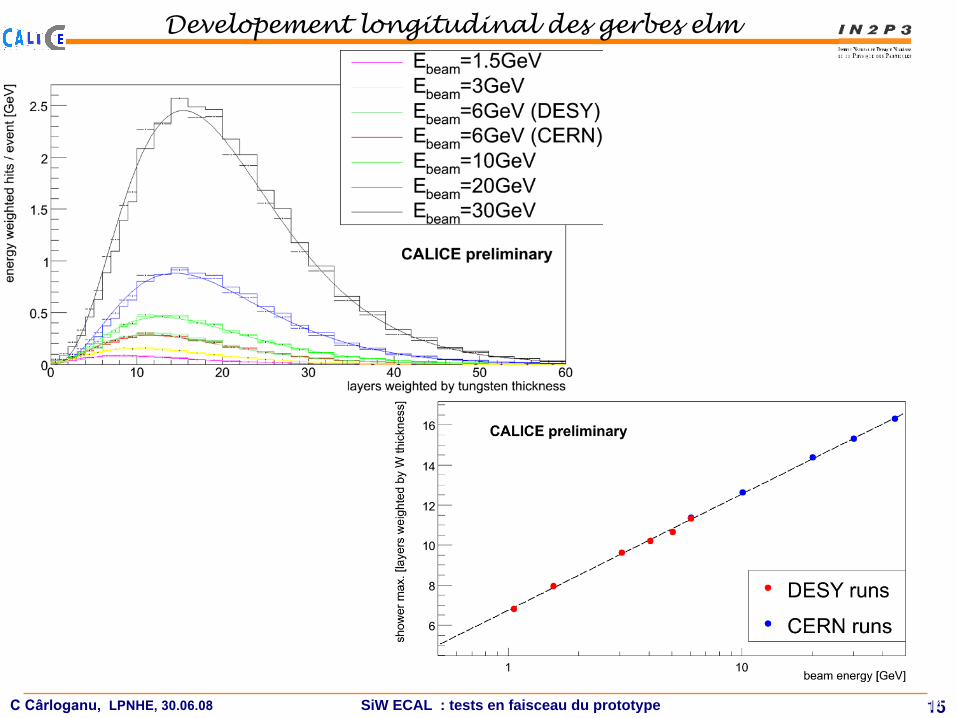
Developement longitudinal des gerbes elm
1514

C Cârloganu, LPNHE, 30.06.08 SiW ECAL : tests en faisceau du prototype
Première étude des pions avec ECAL
1614
17
!"#$%%&'&()*(+,-"./0,1#*
21#3,0"4,#/.(5#6738(9,*07,:"0,1#
;<+= ;<+=>?@A ;<+=>5BC
;<+=>?5!D ;<+=>?5!D>E= ;<+=>E=

18
!"#$%%&'&()*(+,-"./0,1#*
21#3,0"4,#/.(5#6738(9,*07,:"0,1#
2;<=8* >?+; >?+;@25A9
BCB; 2D5< 2D5<@E5!C
C Cârloganu, LPNHE, 30.06.08 SiW ECAL : tests en faisceau du prototype
Première étude des pions avec ECAL
1714
!"#$%&'()*+),-.)*&&' /-012324)5-67-8419()%:;# *<
The 2008 test beam at FNALThe 2008 test beam at FNAL
52=>?-6 -@A)":!"#)-619-A.)2@B8-669A)-8),CD/
E-8-)8-F2@G)B8-189A)4@)HB8 4I),-.)J
C Cârloganu, LPNHE, 30.06.08 SiW ECAL : tests en faisceau du prototype
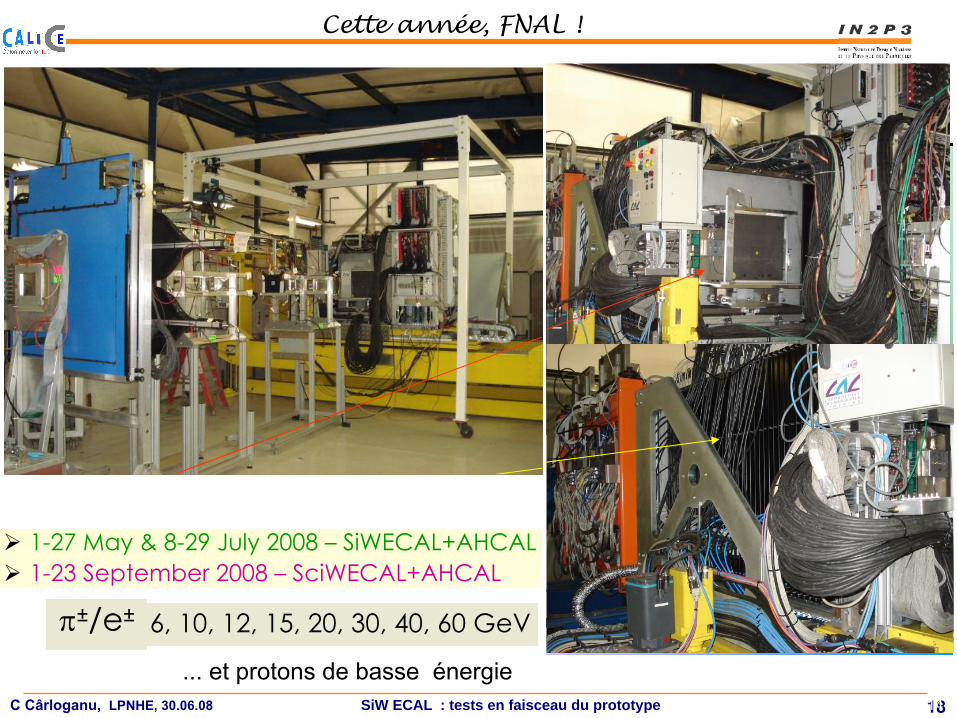
Cette année, FNAL !
1814
!"#$%&'()*+),-.)*&&' /-012324)5-67-8419()%:;# *<
The 2008 test beam at FNALThe 2008 test beam at FNAL
52=>?-6 -@A)":!"#)-619-A.)2@B8-669A)-8),CD/
E-8-)8-F2@G)B8-189A)4@)HB8 4I),-.)J
!"#$%&'()*+),-.)*&&' /-012324)5-67-8419()%:;# *<
Plans for the 2008 test beamPlans for the 2008 test beam
&=)>&()*&()?&)@9A&()>&()*&()?&)@9A"BA69C
D*<,)979B8C)E)'&)F9G)HB-114I)-B@)014-@)09-JK
L,)979B8C)E)>*&)F9G)H014-@)09-JK!-6201-824B)I28M)
! 979B8C
L)84)>'&)F9GL()>&()>*()><()*&()?&()N&()L&)F9GOB91A.)P42B8C
"!Q9! QP"!Q9!R-182S69)8.P9C
"SM2979@)-8)*&&+)!O%T)UVR14P4C9@)P6-B)W41)>C8 P9124@
X UI4)89C8)09-J)P9124@C)E,UV/
! >Y*+),-.)Z)'Y*[)\]6.)*&&')^ 52_O!"#`":!"#
! >Y*?)59P89J091)*&&')^ 5S2_O!"#`":!"#
X R6-B)84)89C8)O!"#`a:!"#)P14848.P9C)2B)CP12BA)*&&[
... et protons de basse énergie
C Cârloganu, LPNHE, 30.06.08 SiW ECAL : tests en faisceau du prototype
Maintenant, au FNAL ...
1914
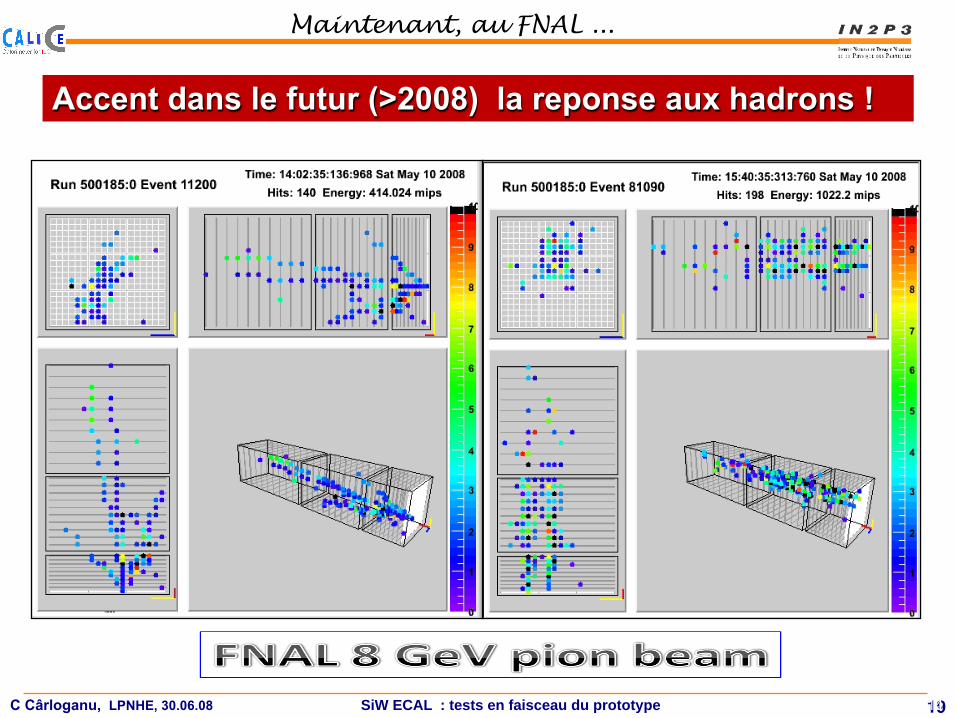
Accent dans le futur (>2008) la reponse aux hadrons !

C Cârloganu, LPNHE, 30.06.08 SiW ECAL : tests en faisceau du prototype
Maintenant, au FNAL ...
2014

C Cârloganu, LPNHE, 30.06.08 SiW ECAL : tests en faisceau du prototype
Conclusion
2114
Quatre laboratoires ( LAL Orsay, LLR Ecole Polytechnique, LPC Clermont, LPSC Grenoble) impliqués dans l’analyse des données.
Un article soumis fin mai sur le comissioning du détecteur (EJPh),
Un article en revue interne CALICE, à soumettre à NIM.
... et six notes internes/publiques CALICE ...
Beaucoup de choses intéressantes à faire, nouvelles contributions bienvenues!