Embed Size (px)
Citation preview

March 6th, 2006 CALICE meeting, UCL 1
Position and angular resolution studies with ECAL TB prototype
IntroductionLinear fit method
Results with 1, 2, 3, and 5 GeV electronsconclusions
Anne-Marie Magnan, IC London.

March 6th, 2006 CALICE meeting, UCL 2
Introduction
o Complete test beam prototype : 30 layers, 1 cm2 cells, 9 wafers per layer.
o Objective : determine position and angular resolution in test beam data, compared with the one obtained in MC simulation.
o Method : linear fit take into account correlations between layers.
o For this study, only 1, 2, 3 and 5 GeV single electrons
(DESY test beam).
o Own generation with Mokka05.05.
Beam position and RMS : (0 ±10, 0 ± 10, -220 ± 0) (in mm).
Current LCIO output does not allow to have the “truth” position in 1st ECAL layer after scattering in air/trackers materials.
March 6th, 2006 CALICE meeting, UCL 3
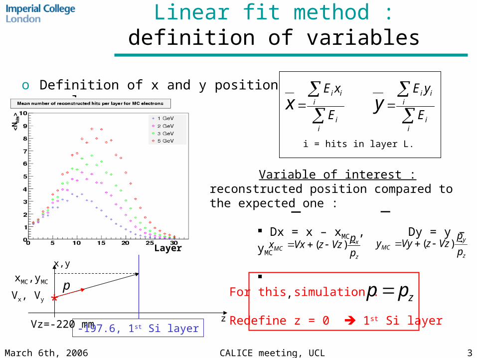
Linear fit method : definition of variables
o Definition of x and y position per layer :
ii
iii
E
xEx
ii
iii
E
yEy
i = hits in layer L.
zVz=-220 mm
x,y
*Vx, Vy
-197.6, 1st Si layer
pxMC,yMC
Variable of interest : reconstructed position compared to the expected one :
Dx = x – xMC , Dy = y – yMC
,z
xMC p
pVzzVxx
)(
z
yMC p
pVzzVyy
)(
_ _
For this simulation :
Redefine z = 0 1st Si layer
zpp
Layer

March 6th, 2006 CALICE meeting, UCL 4
Linear fit method : definition of the χ2
o Estimator of how accurate the prediction of the measurement is :• Without correlations between
variables :
• With correlations between variables :
• Wij is the inverse of the error matrix Eij :
2
22 )(
ltheoreticameasured xx
zppx xxltheoretica 10
jthmeasijiji
thmeas xxWxx )()(,
2
y
xx
i,j = 1,.....,30 for x 31,.....,60 for y
jijijijiij DxDxDxDxDxDxDxDxE ),cov(
= 0

March 6th, 2006 CALICE meeting, UCL 5
Error matrix(= covariance matrix)
Error matrix normalized on the diagonal values(= correlation matrix)
Linear fit method : error matrix
o Wij is calculated thanks to the whole sample (25,000 electrons)
x
y
x y
x
y
x y
No significant correlations
between x and y
1 GeV
Funny pattern : due to non-overlapping layers in x ???
Layer
Diagonal termsDiagonal terms

March 6th, 2006 CALICE meeting, UCL 6
Error matrix for higher energies
2 GeV 3 GeV 5 GeV

March 6th, 2006 CALICE meeting, UCL 7
Linear fit method : minimisation of the χ2
o X and y are uncorrelated : we consider 2 (30,30) matrices
2 independent fits : one for x, the other for y.
we can then look for the parameters (p0x,p1x) of the linear fit which minimize the χ2 :
00
2
xp
0
1
2
xp
x = x or y
Reminder : jthmeasijiji
thmeas xxWxx )()(,
2
zppx xxltheoretica 10
-1
=
2
2
110
100
xxx
xxx
ppp
ppp
jiij
iij
x
x
jiijiij
iijij
xzW
xW
p
p
zzWzW
zWW
1
0
o This gives the following equation :

March 6th, 2006 CALICE meeting, UCL 8
Linear fit method : expected resolution
σp0x (mm) σp0y (mm) σp1x (mrad) σp1y (mrad)
1 GeV 2.4 2.8 58 60
2 GeV 2.4 2.8 48 50
3 GeV 2.3 2.7 41 44
5 GeV 2.2 2.5 35 37
z-220 mm
x,y
*
-197.6, 1st Si layer
p
p0
p1σp0
σp1
o Angular resolution decrease when E increase :more layers on the back better constraintso Position resolution decrease as well when E increase : more hits better estimate of the average positiono Position resolution is higher in y , why ???????
Best case : if all layers
!!+ tracker resolution!!!! in data !!
Best case : if all layers

March 6th, 2006 CALICE meeting, UCL 9
Position and angular resolutionobtained on an event by event basis
Therefore have to solve it event by event.
jiij
iij
x
x
jiijiij
iijij
xzW
xW
p
p
zzWzW
zWW
1
0
To solve this, need to take into account only layers i and j with hits remove layers with no hit from error matrix, then invert to have W matrix.
Equation to solve :

March 6th, 2006 CALICE meeting, UCL 10
Results event by event for parameter resolution matrices
xp1
yp1
xp0
yp0
=
2
2
110
100
xxx
xxx
ppp
ppp
-1
jiij
iij
x
x
jiijiij
iijij
xzW
xW
p
p
zzWzW
zWW
1
0

March 6th, 2006 CALICE meeting, UCL 11
Result event by eventfor (p0 – p0MC)x,y
x y
Energy σp0x (mm) if all layers σp0y (mm) if all layers
1 GeV 2.6 2.4 3.1 2.8
2 GeV 2.5 2.4 2.9 2.8
3 GeV 2.4 2.3 2.8 2.7
5 GeV 2.2 2.2 2.6 2.5

March 6th, 2006 CALICE meeting, UCL 12
Result event by eventfor (p1 – p1MC)x,y
x y
Energy σp1x (mrad) if all layers σp1y (mrad) if all layers
1 GeV 71 58 74 60
2 GeV 54 48 56 50
3 GeV 45 41 48 44
5 GeV 36 35 39 37

March 6th, 2006 CALICE meeting, UCL 13
Consistency checks
o Pull of the distributions for Δp0 (=p0 – p0MC) and Δ p1
xp
xp
0
0
yp
yp
0
0
xp
xp
1
1
yp
yp
1
1
0.88-0.96 0.96-0.99
0.95-0.97 0.97-0.98

March 6th, 2006 CALICE meeting, UCL 14
With material in front of ECAL
o Beam position : (4,7,10000) mm
o Expected effect of air scattering in 10 m ~ 13 mm spread.
o Observed <x> : ~ 16 mm spread.
o Expected resolution :• The “true” position is now given by
hits in last DC layer
• σp0x = 5.2 mm, σp0y = 5.3 mm
• σp1x = 70 mrad, σp1y = 69 mrad
still correlations. Need to have the “true” position of MC particle at front ECAL face.
1 GeV

March 6th, 2006 CALICE meeting, UCL 15
Future work
o Study with missing layers : better to have front, middle, back ? First layers needed for position resolution, and last ones for angular resolution… but depend on energy.
Hakan + AM
o Redo everything with material in front, and truth entry point.
o Study of reconstructed tracking resolution to separate the 2 sources and allow to compare with data.
o Redo everything when realistic digitisation is available.

March 6th, 2006 CALICE meeting, UCL 16
Thank you for your attention