Embed Size (px)
Citation preview

Short-Term Scheduling under Uncertainty
Marianthi Ierapetritou
Department Chemical and Biochemical Engineering
Piscataway, NJ 08854-8058

Sandia National LaboratoriesLarge-Scale Robust Optimization
Objective
Identify and reduce bottlenecks at different levels
Integration of the whole decision-making process
Online Control
Short-term Scheduling
Production Planning
Supply Chain Management
Time Horizon
Uncertainty Complexity
Opportunity for
Optimization
Process Operations Decision Making

Sandia National LaboratoriesLarge-Scale Robust Optimization
Short-term scheduling Uncertainty in product prices, product demands, raw material
availability, machine availability, processing times
Production Planning Longer time horizon under consideration (several months) Larger number of materials and products Uncertainty in facility availability, product demands, orders, raw
materials
Supply chain management Multiple sites involving production, inventory management,
transportation Longer planning time horizon (couple of years) Uncertainty in material availability, costs, transportation
Uncertain Parameters

Sandia National LaboratoriesLarge-Scale Robust Optimization
Process Plant Optimal Schedule
Given: Determine:Raw Materials, Required Products, Task Sequence, Production Recipe, Unit Capacity Exact Amounts of
materialProcessed
Scheduling objectives : Economic Maximize Profit, Minimize Operating Costs,
Minimize Inventory CostsTime Based Minimize Makespan, Minimize Tardiness
Short-term Scheduling

Sandia National LaboratoriesLarge-Scale Robust Optimization
Binary variables to allocate tasks to resources
Continuous variables to represent timing and material variables
Mixed Integer Linear Programming Models
Smaller models that are computationally efficient and tractable
T2T2T1 T1
T1 T2 T2 T1 T2 T2 T2T1
Discrete time formulation
“Real” time schedule
Continuous time formulation
Event Points: When a tasks begins
Continuous Time Formulation

Sandia National LaboratoriesLarge-Scale Robust Optimization
Deterministic Scheduling Formulation
minimize H or maximize price(s)d(s,n)
subject to wv(i,j,n) 1
st(s,n) = st(s,n-1) – d(s,n) + Pb(i,j,n-1) +
cb(i,j,n)
st(s,n) stmax(s)
Vmin(i,j)wv(i,j,n) b(i,j,n) Vmax(i,j)wv(i,j,n)
d(s,n) r(s)
Tf(i,j,n) = Ts(i,j,n) + (i,j)wv(i,j,n) + (i,j)b(i,j,n)
Ts(i,j,n+1) Tf(i,j,n) – U(1-wv(i,j,n))
Ts(i,j,n) Tf(i’,j,n) – U(1-wv(i’,j,n))
Ts(i,j,n) Tf(i’,j’,n) – U(1-wv(i’,j’,n))
Ts(i,j,n) H, Tf(i,j,n) H
Duration Constraints
Demand Constraints
Allocation Constraints
Capacity Constraints
Material Balances
Objective Function
n
s
(i,j)
M.G.Ierapetritou and C.A.Floudas. Effective continuous-time formulation for short-term scheduling. 1. Multipurpose batch processes. 1998

Sandia National LaboratoriesLarge-Scale Robust Optimization
Increased Complexity: Parameter Fluctuations

Sandia National LaboratoriesLarge-Scale Robust Optimization
Price of P1 is an uncertain parameter. Considering time horizon of 16 hours, $1 increase results in the following different production schedules.
Uncertainty impacts the optimal schedule
Uncertainty in Short-Term Scheduling

Sandia National LaboratoriesLarge-Scale Robust Optimization
0 82 4 61 3 5 7
0 82 4 61 3 5 7
50.00
50.00
10.40
64.60 10.03 50.93
64.04 4.63 50.93
55.56
74.07 4.63 50.93
44.44 74.07 50.93
55.56 Deterministic Schedule
Deterministic Schedule
Robust ScheduleRobust
Schedule
heating
heating
reaction 1 reaction 2 reaction 3 reaction 2
reaction 1 reaction 2 reaction 3
separation
reaction 2 reaction 2reaction 3
reaction 3reaction 1 reaction 1
separation
demand (product 2) = 50*(1 + 60%)
demand (product 2) = 50
Standard Deviation = 0.29
E(makespan) = 7.24hr
E(makespan) = 8.15hr
Standard Deviation = 2.63
Uncertainty in Short-Term Scheduling

Sandia National LaboratoriesLarge-Scale Robust Optimization
Literature Review: Representative Publications
Reactive Scheduling
S.J.Honkomp, L.Mockus, and G.V.Reklaitis. A framework for schedule evaluation with processing uncertainty. Comput. Chem. Eng. 1999, 23, 595 J.P.Vin and M.G.Ierapetritou. A new approach for efficient rescheduling of multiproduct batch plants. Ind. Eng. Chem. Res., 2000, 39, 4228
Handles uncertainty by adjusting a schedule upon realization of the uncertain parameters or occurrence of unexpected events
Stochastic ProgrammingUncertainty is modeled through discrete or continuous probability functions J.R.Birge and M.A.H.Dempster. Stochastic programming approaches to stochastic scheduling. J. Global. Optim. 1996, 9, 417 J.Balasubramanian and I.E.Grossmann. A novel branch and bound algorithm for scheduling flowshop plants with uncertain processing times. Comput. Chem. Eng. 2002, 26, 41

Sandia National LaboratoriesLarge-Scale Robust Optimization
Literature Review: Representative Publications
Robust Optimization
X.Lin, S.L.Janak, and C.A.Floudas. A new robust optimization approach for scheduling under uncertainty – I. bounded uncertainty. Comput. Chem. Eng. 2004, 28, 2109
Produces “robust” solutions that are immune against uncertainties
Fuzzy Programming
H.Ishibuchi, N.Yamamoto, T.Murata and Tanaka H. Genetic algorithms and neighborhood search algorithms for fuzzy flowshop scheduling problems . Fuzzy Sets Syst. 1994, 67, 81 J.Balasubramanian and I.E.Grossmann. Scheduling optimization under uncertainty- an alternative approach. Comput. Chem. Eng. 2003, 27, 469
Considers random parameters as fuzzy numbers and the constraints are treated as fuzzy sets
MILP Sensitivity Analysis
Z.Jia and M.G.Ierapetritou. Short-term Scheduling under Uncertainty Using MILP Sensitivity Analysis. Ind. Eng. Chem. Res. 2004, 43, 3782
Utilizes MILP sensitivity analysis methods to investigate the effects of uncertain parameters and provide a set of alternative schedules

Sandia National LaboratoriesLarge-Scale Robust Optimization
Disruptive EventsRush Order ArrivalsOrder CancellationsMachine Breakdowns
Not much informatio
n is
available
REACTIVESCHEDULING
Parameter UncertaintyProcessing timesDemand of productsPrices
Information is available
PREVENTIVE SCHEDULING
Uncertainty in Scheduling

Sandia National LaboratoriesLarge-Scale Robust Optimization
model robustness
solution robustness
Data perturbation
New alternative schedules
Deterministic schedule
LB/UB on objective function
MILP
sensitivity
analysis
framework
Robust
optimization
method
A set of solutions represent trade-off between various
objectives
Preventive Scheduling

Sandia National LaboratoriesLarge-Scale Robust Optimization
Preventive Scheduling
Robust Optimization
MILP Sensitivity
Analysisminimize H or maximize price(s)d(s,n)
subject to wv(i,j,n) 1st(s,n) = st(s,n-1) – d(s,n) + Pb(i,j,n-1) + cb(i,j,n)
st(s,n) stmax(s) Vmin(i,j)wv(i,j,n) b(i,j,n) Vmax(i,j)wv(i,j,n)
d(s,n) r(s) Tf(i,j,n) = Ts(i,j,n) + (i,j)wv(i,j,n) + (i,j)b(i,j,n)
Ts(i,j,n+1) Tf(i,j,n) – U(1-wv(i,j,n))Ts(i,j,n) Tf(i’,j,n) – U(1-wv(i’,j,n))Ts(i,j,n) Tf(i’,j’,n) – U(1-wv(i’,j’,n))
Ts(i,j,n) H, Tf(i,j,n) H
Mixed-Mixed-integer integer Linear Linear
ProgramminProgrammingg

Sandia National LaboratoriesLarge-Scale Robust Optimization
mixing
reaction
separation
H (time horizon)100 2 4 8
55
55
50
mixing
reaction15
6
15
20separation
-Can the schedule accommodate the demand fluctuation?
-How the capacity of the units affect the production objective?
- What is the effect of processing time at the objective value?
Questions to Address

Sandia National LaboratoriesLarge-Scale Robust Optimization
Inference-based MILP Sensitivity Analysis
iP Aijuj
P + sj(uj – uj) - iai rP
sjP i
PAij, sjP -qj
P, j = 1,…,n
rP = -qjPuj
P + Pa – zP +zP
cjujP - sj
P(ujP – uj
P) -rP
sjP -cj, sj
P -qjP, j = 1,…,n
qjP = i
PAij - iPcj
- for the perturbations - for the perturbations A and A and a a - for the perturbations - for the perturbations c c
Bound z z* - z holds if there are s1P,…,sn
P that satisfy:
minimize z = cxsubject to Ax a
0 x h, xj integer, j=1,…k
minimize z = (c + cc)xsubject to (A + AA)x a + aa
0 x h, xj integer, j=1,…k
Aim: Determine under what condition z z* - z remains valid
Partial assignment at node pxj {ujP,…,uj
P} j = 1,…,n
*M.W.Dawande and J.N.Hooker, 2000

Sandia National LaboratoriesLarge-Scale Robust Optimization
Extract information from
the leaf nodes
Extract information from
the leaf nodes
Solve the deterministic scheduling problem using
B&B tree
Solve the deterministic scheduling problem using
B&B tree
Proposed Uncertainty Analysis Approach
- Range of objective
change for certain parameter change
- Range of objective
change for certain parameter change
Solve relaxed LP at the leaf nodes with perturbed data
Solve relaxed LP at the leaf nodes with perturbed data
Identify the feasible schedules by examining the
B&B tree
Identify the feasible schedules by examining the
B&B tree
Evaluate the alternative schedules
Evaluate the alternative schedules
- Robustness- Nominal performance- Average performance
- Robustness- Nominal performance- Average performance
MILP Sensitivity MILP Sensitivity AnalysisAnalysis

Sandia National LaboratoriesLarge-Scale Robust Optimization
Obtain sequence of tasks
from original schedule
42
56
70
84
98
33 44 55 66 77
P1
P2
Generate random demands in expected
range
Makespan minimization is considered as the objective
Makespan to meet a particular demand is found using the sequence of tasks derived from original scheduleBinary variables corresponding to allocation of tasks are fixedBatch sizes and Starting and Finishing times of tasks are allowed to vary
Robustness Estimation

Sandia National LaboratoriesLarge-Scale Robust Optimization
Inventory ofraw materialsintermediates
etc.
Hmax HinfROLLOVER
Meets maximum possibledemand
Meets unsatisfieddemand
Total makespan Hcorr = Hmax + HinfCorrected Standard Deviation:
Hact = Hp if scenario is feasible = Hcorr if the scenario is infeasible
totp
p tot
actcorr p
HHSD
1
2det
)1(
)(
Robustness under Infeasibility
J.P.Vin and M.G.Ierapetritou. Robust short-term scheduling of multiproduct batch plants under demand uncertainty. 2001

Sandia National LaboratoriesLarge-Scale Robust Optimization
Case Study 1
S1S1 S2S2 S3S3 S4S4
wv(i1,j1,n0)
wv(i1,j1,n1)
wv(i2,j2,n1)
wv(i3,j3,n2)
wv(i2,j2,n2)
3.0
5.17 3.0
7.65 5.83 7.16infeasible
8.14 10.16 7.16
9.83infeasible
infeasible8.33
9.87 8.83
7.16
8.839.98
infeasible
9.83
(Schedule 1)
0
00
0
0 0 0 0
00
1
1
1
1 1
1 1
1
11
Effect of demand d~[20, 100]
-0.097 d Hdnom = 50
H’ Hnom + 0.097d = 12.73hd’ = 80
Hnom = 9.83h
mixingmixing reactionreaction purificationpurification
B&B tree with B&B tree with nominal nominal demanddemand

Sandia National LaboratoriesLarge-Scale Robust Optimization
Case Study 1
(Schedule 2) (Schedule 3)
0
0 0
01
1 1
1(12.13)
schedule 1 schedule 2 schedule 3
Hnom(h)
Havg(h)
SDcorr
9.83
14.20
5.52
10.77
11.56
1.61
10.91
11.79
2.17
wv(i1,j1,n0)
wv(i1,j1,n1)
wv(i2,j2,n1)
wv(i3,j3,n2)
wv(i3,j3,n3)
wv(i2,j2,n2)
3.0
5.17 3.0
7.65 5.83 7.16infeasible
8.14 10.16 7.16
9.83infeasible
infeasible8.33
9.87 8.83
7.16
8.839.98infeasible
9.83
(Schedule 1)
0
00
0
0 0 0 0
00
1
1
1
1 1
1 1
1
11
(12.73)(17.97)
Schedule Schedule EvaluationEvaluation

Sandia National LaboratoriesLarge-Scale Robust Optimization
5
7
9
11
13
15
20 30 40 50 60 70 80 90 100
Demand
H
schedule 1 (optimal when d ≤ 50)
schedule 2 (optimal when d ≥ 50)
schedule 3
Case Study 1

Sandia National LaboratoriesLarge-Scale Robust Optimization
Case Study 1Effect of processing time T(i1,j1) ~ [2.0, 4.0]
profit’ profitnom + 24.48T = 47.04Tnom = 3.0
T’ = 4.0
profitnom = 71.52
schedule 1schedule 2 schedule 3
profitnom
profitavg
SDcorr
71.52
66.98
26.9
65.27
9.33
65.27
65.17
10.49
wv(i1,j1,n0)
wv(i1,j1,n1)
wv(i2,j2,n1)
wv(i3,j3,n2)
wv(i3,j3,n3)
wv(i2,j2,n2)
100
100 50
100
100 96.05
78.42
50
(75)
0
0
0
0
0
0
0
1
1
1
1
1
1
1
71.52
100
50
75
(Schedule 1)
50
75(75)
1 050
72.46(62.11)
78.42
64.61
(Schedule 2)
1 0
1
0
1
1
1
1 0
(Schedule 3)

Sandia National LaboratoriesLarge-Scale Robust Optimization
Shortcoming of Proposed Approach
Since the entire analysis is based on a single tree among a large number of possible branch-and-bound trees that can be used to solve the MILP, it provides conservative sensitivity ranges.

Sandia National LaboratoriesLarge-Scale Robust Optimization
Parametric Programming
z() = min cTx + dTysubject to Ax + Dy
bxL x xU
L U
x Rm, y (0,1)T
z() = min cTx + dTysubject to Ax + Dy - r b
cTx + dTy – z0 - = 0
yi - yi F1 - 1
xL x xU
L’ U’x Rm, y (0,1)T
iF1 iF 0
b = b0 + r
LP sensitivity analysis: z() = z0 +
L L’ U’ U
solved at b = b0+Lr
optimal solution (x*,y*)
Integer cut to exclude current optimal solution
b[b0+Lr, b0+Ur]
break point ’, new optimal solution (x*’,
y*’)
Fix integer variables at y*
A.Pertsinidis et al. Parametric optimization of MILP programs and a framework for the parametric optimization of MINLPs. 1998

Sandia National LaboratoriesLarge-Scale Robust Optimization
Multiparametric MILP
J. Acevedo and E.N.Pistikopoulos. A Multiparametric Programming Approach for Linear Process Engineering Problems under Uncertainty. 1997
Select a branching variable
Select a branching variable
Solve the fully relaxed problem
Solve the fully relaxed problem
Solve the mpLP at the
nodes
Solve the mpLP at the
nodes
Compare the solution with the current UB, update the optimal function in the uncertain space
Compare the solution with the current UB, update the optimal function in the uncertain space
Based on simplex algorithm, check the neighboring bases of the LP
tableau
Based on simplex algorithm, check the neighboring bases of the LP
tableau

Sandia National LaboratoriesLarge-Scale Robust Optimization
Shortcomings of Existing Approach
mpLP approach requires retrieving the LP
tableaus and visiting the neighbor bases
Solve mpLP at every node in the B&B tree during
the branch and bound procedure: can be a
computationally expensive effort

Sandia National LaboratoriesLarge-Scale Robust Optimization
Proposed Analysis on the RHS for MILPs
minimize z = cxsubject to Ax a x 0, xj Є (0, 1), j=1,…k
minimize z = cxsubject to Ax a + ax 0, xj Є (0, 1) , j=1,…k
Develop a framework to investigate the effect of Δa on the optimal solution x and objective value z
A set of optimal integer solutions Critical regions Optimal functions

Sandia National LaboratoriesLarge-Scale Robust Optimization
Proposed Approach: Single Uncertain Parameter
Find Δamax that leaves the structure of the
tree unchanged
Find Δamax that leaves the structure of the
tree unchanged
Solve the original problem at the nominal value using
a branch and bound method
Solve the original problem at the nominal value using
a branch and bound method
Collect zp, λp at each leaf node
p
Collect zp, λp at each leaf node
p
For a = Δamax + ε update the B&B treeFor a = Δamax + ε
update the B&B tree

Sandia National LaboratoriesLarge-Scale Robust Optimization
Δamax = min{Δabasis, min{ } }zp – z0
λp – λ0
Case 1: A descent node of the node 0
Case 2: A descent node of other leaf node
Case 3: Node 0, but the basis has changed
The new optimal node can be:
Determine Δamax and Update the B&B Tree
P
Update the B&B tree at a = Δamax +ε
where node 0 is the optimal node
0
*
case
1
*
case
2
case
3

Sandia National LaboratoriesLarge-Scale Robust Optimization
Proposed Approach: Multiple Uncertain Parameters
mpLP at the leaf nodes
mpLP at the leaf nodes
mpLP algorithm
mpLP algorithm
Compare the critical regions with the current upper bounds Update the B&B tree
Compare the critical regions with the current upper bounds Update the B&B tree
Solve the original problem at the nominal value using
a branch and bound method
Solve the original problem at the nominal value using
a branch and bound method

Sandia National LaboratoriesLarge-Scale Robust Optimization
mpLP Algorithm at the Leaf Nodes
maximize cx* – zsubject to z = max{z(k) + λ(k)θa + β(k)θb}
a0 ≤ θa ≤ a0 + Δa
b0 ≤ θb ≤ b0 + Δb
Bilevel Linear Programming
At each iteration, solve
where x* = argmin cxsubject to Ax ≥ θ
θ
cx*
max{z(k) + λ(k)θ}
cx*current optimal functions
Sandia National LaboratoriesLarge-Scale Robust Optimization
mpLP Algorithm at the Leaf Nodes
maximize {min cx| Ax θ} – z
subject to z z(k) + λ(k)θa + β(k)θb
a0 ≤ θa ≤ a0 + Δa
b0 ≤ θb ≤ b0 + Δb
current optimal functions
check if there is any point at which max{z(k) + λ(k)θa + β(k)θb} is less than cx*
Stop when the objective = 0
Include an additional constraint z z(k+1) + λ(k+1)θa + β(k+1)θb to above problem

Sandia National LaboratoriesLarge-Scale Robust Optimization
Solve the Bilevel Programming Problem
max θys.t. ATy ≤ c a0 ≤ θa ≤ a0 + Δa
b0 ≤ θb ≤ b0 + Δb
Y 0
min cxs.t. Ax θ a0 ≤ θa ≤ a0 + Δa
b0 ≤ θb ≤ b0 + Δb
x 0
Replace the inside optimization problem by its dual
max θy - zs.t. ATy ≤ cz z(k) + λ(k)θa + β(k)θb
a0 ≤ θa ≤ a0 + Δa
b0 ≤ θb ≤ b0 + Δb
Y 0
Single optimization
problem
Convert the relaxed LP to its dual
formStrong Duality
Theorem
Bilinear objective Linear constraints
Solve with global optimization solver
BARON

Sandia National LaboratoriesLarge-Scale Robust Optimization
Compare the Optimal Functions of the Leaf Nodes
z1UB = z1
*UB + λ1UBθa + β1
UBθb
1
2
z2(2) = z2
*(2) + λ2(2)θa + β2
(2)θb
CR2(2)CR2
(1)
CR2(3)
CR1(1) CR1
UB
CR1UB CR2
(2) = CRint

Sandia National LaboratoriesLarge-Scale Robust Optimization
Compare the Optimal Functions of the Leaf Nodes
min Єs.t. z1
UB = z2(2) + Є
z1UB = z1
*UB + λ1UBθa + β1
UBθb
z2(2) = z2
*(2) + λ2(2)θa + β2
(2)θb
θa,θb Є CRint
Redundancy test
on constraint z1UB ≥
z2(2)
Case 1: Problem is infeasible: z1UB is smaller in
CRintCase 2: Є > 0: the constraint is redundant. z2
(2) is smaller in CRint The optimal function is updated to be z2
(2) if node 2 is an integer node, otherwise, do not update.
Compare optimal function z1UB and z2
(2) in region CRint
Case 3: Є < 0: the constraint is not redundant. CRint is divided into two parts. z1
UB is smaller on one side and z2(2) is
smaller on the other side. The two regions are divided by z1
UB ≤ z2(2).

Sandia National LaboratoriesLarge-Scale Robust Optimization
Advantage of Proposed Approach
The new mpLP approach can efficiently determine the
optimal functions and critical regions without retrieving the
LP tableaus and visiting the neighbor bases
Solve mpLP at only the leaf nodes in the B&B tree instead
of every node during the branch and bound procedure –
reduce the computational efforts significantly

Sandia National LaboratoriesLarge-Scale Robust Optimization
Case Study: Single Uncertain Parameter
min z = 2x1 + 3x2 + 1.5x3 + 2x4 + 0.5x5
s.t. 2x1 + x2 + x3 ≥ 7 + Δa
2x2 + x4 + x5 ≥ 4
x3 + x4 – x5 ≥ 0
2x1 – x2 – x3 + x5 ≥ 4
1≤ x ≤ 3, xj Є (0,1), j = 3,4,5
Step 1:
3
2
x3 = 1 x3 = 0
x4 = 1 x4 = 0
0
12
11.5* 12(0,1,1)
Step 2: Linear sensitivity analysis on node 0 -- Δamax = 0
Step 3: For Δa = Δamax + ε, node 0 yields noninteger solution. Update the B&B tree.
Δa = 0

Sandia National LaboratoriesLarge-Scale Robust Optimization
3
2
x3 = 1 x3 = 0
x4 = 1 x4 = 0
0
12
11.8*
12
λ = 3
x5 = 1 x5 = 0
12.1
3
2
x3 = 1 x3 = 0
1 0
012.2
12.1 12*
1 0
12.2
1 1 00
12*4
5
λ = 0
λ = 0
λ = 1
λ = 1 λ = 2
Step 2:
Δamax = min{Δabasis, min{ } }zp – z0
λp – λ0P
= min{ 2, min { }}0.32 ,
0.23 ,
0.23
0.23
=
Step 3:
For Δa = Δamax + ε, node 0 is intersected by node 2 & 3. Update the B&B tree
Step 3:
Step 2: ...
...
Case Study: Single Uncertain Parameter

Sandia National LaboratoriesLarge-Scale Robust Optimization
0 0.2 0.4 0.6 0.8 1.0 1.2 1.4 1.6 1.8 211.5
12
12.5
13
13.5
14
(0,1,1)
(1,0,1) & (0,0,0)
(1,0,1)
(1,0,1)
Final optimal solution:
z*
Δa
Case Study: Single Uncertain Parameter

Sandia National LaboratoriesLarge-Scale Robust Optimization
Case Study: Multiple Uncertain Parameters
min z = -3x1 - 8x2 + 4y1 + 2y2
s.t. x1 + x2 ≤ 13 + θ1
5x1 - 4x2 ≤ 20
-8x1 + 22x2 ≤ 121 + θ2
4x1 + x2 ≥ 8
x1 – 10y1 ≤ 0
x2 – 15y3 ≤ 0
x ≥ 0, y Є (0,1), 0 ≤ θ1,θ2 ≤ 10Step 1:
1
y1 = 0 y1 = 1
y2 = 0 y2 = 1
2-8 -70.5*
(θ1, θ2) = (0, 0)

Sandia National LaboratoriesLarge-Scale Robust Optimization
max (-13-θ1)d1 – 20d2 + (-121-θ2)d3 + 8d4 – d7 – d8 - zs.t. -d1 – 5d2 + 8d3 + 4d4 – d5 ≤ -3
-d1 + 4d2 – 22d3 + d4 – d6 ≤ -8
10d5 – d7 ≤ 4
15d6 – d8 ≤ 2
z ≥ -70.5 – 4.3333θ1 – 0.1667θ2
0 ≤ θ1, θ2 ≤ 10
Step 2: mpLP on the leaf nodes
Node 1z1
(1) = -70.5 – 4.3333θ1 – 0.1667θ2 at (θ1, θ2) = (0, 0)
obj = 16.74 (θ1, θ2) = (10, 0)
z1(2) = -97.0909 – 0.1667θ2 at (θ1, θ2) = (10, 0)
Case Study: Multiple Uncertain Parameters

Sandia National LaboratoriesLarge-Scale Robust Optimization
max (-13-θ1)d1 – 20d2 + (-121-θ2)d3 + 8d4 – d7 – d8 - zs.t. -d1 – 5d2 + 8d3 + 4d4 – d5 ≤ -3
-d1 + 4d2 – 22d3 + d4 – d6 ≤ -8
10d5 – d7 ≤ 4
15d6 – d8 ≤ 2
z ≥ -70.5 – 4.3333θ1 – 0.1667θ2
z ≥ -97.0909 – 0.3636θ2
0 ≤ θ1, θ2 ≤ 10obj = 0, stop
z1(1) ≥ z1
(2) 0.07333θ1 – 0.00333θ2 ≤ 0.45
The two critical regions are divided by
Case Study: Multiple Uncertain Parameters

Sandia National LaboratoriesLarge-Scale Robust Optimization
Node 2 z2 = 8
CR2 =θ1 ≤ 10
θ2 ≤ 10
Step 3: Compare critical regions and determine optimal functions
0.07333θ1 – 0.00333θ2 ≤ 0.45
θ2 ≤ 10
z1(1) = -70.5 – 4.3333θ1 –
0.1667θ2
CR1(1)
=
z1(2) = -97.0909 – 0.3636θ2
0.07333θ1 – 0.00333θ2 ≥ 0.45
θ1, θ2 ≤ 10CR1
(2) =
CR1(1) and CR2
CR1(1) n CR2 = CR1
(1)
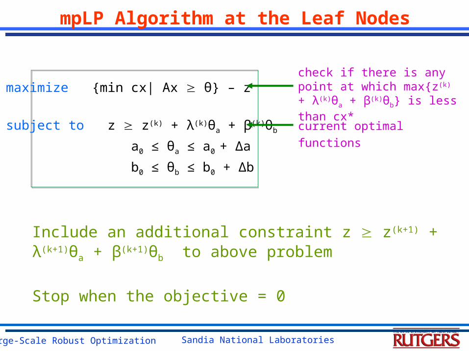
Case Study: Multiple Uncertain Parameters
Sandia National LaboratoriesLarge-Scale Robust Optimization
min Єs.t. -97.0909 – 0.3636θ2 + Є = -8
0.07333θ1 – 0.00333θ2 ≥ 0.45
0 ≤ θ1, θ2 ≤ 10
Є > 0,z1
(2) ≤ z2 is redundant in CR1
(2)
min Єs.t. -70.5 – 4.3333θ1 - 0.1667θ2 + Є = -8
0.07333θ1 – 0.00333θ2 ≤ 0.45
θ2 ≤ 10
Є < 0, z1(1) ≤ z2
CR1(2) and CR2
CR1(2) n CR2 = CR1
(2)
CR1(1)
CR1(2)
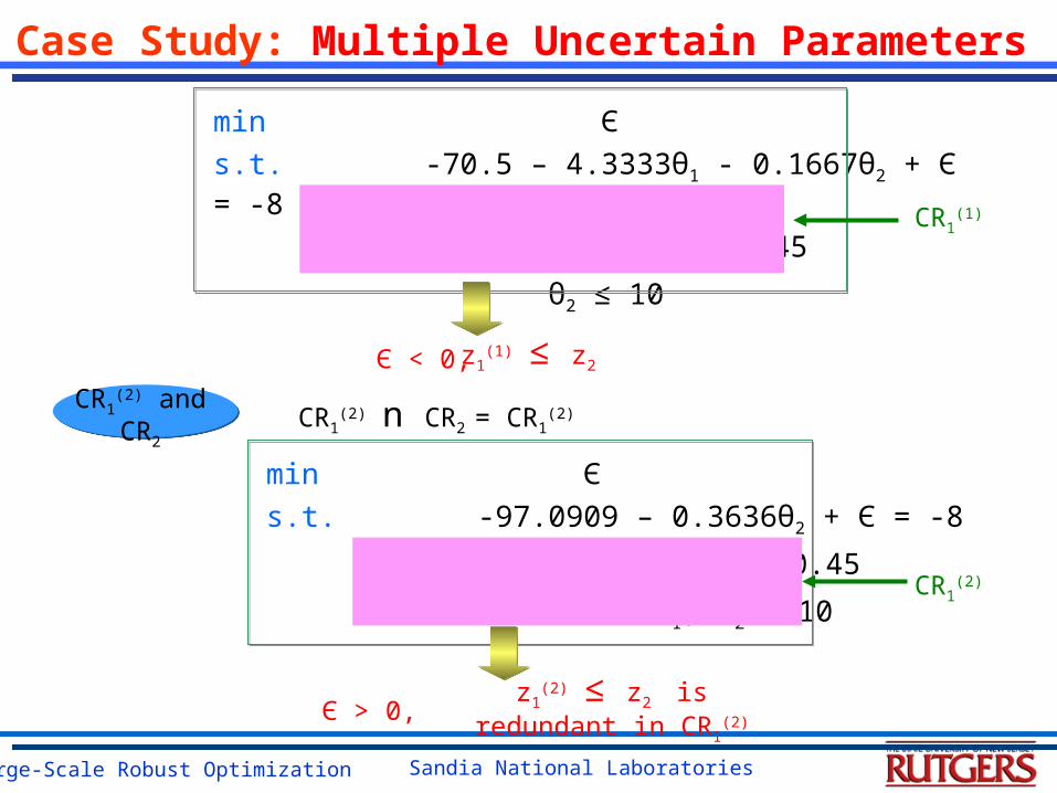
Case Study: Multiple Uncertain Parameters
Sandia National LaboratoriesLarge-Scale Robust Optimization
0.07333θ1 – 0.00333θ2 ≤ 0.45
θ2 ≤ 10
z1(θ) = -70.5 – 4.3333θ1 – 0.1667θ2
CR1(1)
=
z2(θ) = -97.0909 – 0.3636θ2
0.07333θ1 – 0.00333θ2 ≥ 0.45
θ1, θ2 ≤ 10CR1
(2) =
y* = (1, 1)
Final optimal solution:
Case Study: Multiple Uncertain Parameters
Sandia National LaboratoriesLarge-Scale Robust Optimization
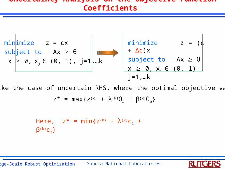
Uncertainty Analysis on the Objective Function Coefficients
minimize z = cxsubject to Ax θ x 0, xj Є (0, 1), j=1,…k
minimize z = (c + Δc)xsubject to Ax θx 0, xj Є (0, 1) , j=1,…k
z* = max{z(k) + λ(k)θa + β(k)θb}
Unlike the case of uncertain RHS, where the optimal objective value
Here, z* = min{z(k) + λ(k)c1 + β(k)c2}

Sandia National LaboratoriesLarge-Scale Robust Optimization
maximize z – (c + Δc)x subject to Ax ≥ θ
z ≤ z(k) + λ(k)c1 + β(k)c2
c10 ≤ c1 ≤ c10 + Δc1
c20 ≤ c2 ≤ c20 + Δc2
mpLP Algorithm at the Leaf Nodes
maximize z – (c + Δc)x* subject to z = min{z(k) + λ(k)θa + β(k)θb}
c10 ≤ c1 ≤ c10 + Δc1
c20 ≤ c2 ≤ c20 + Δc2
Bilevel Linear Programming
where x* = argmin (c+Δc)xsubject to Ax ≥ θ
One level NLP

Sandia National LaboratoriesLarge-Scale Robust Optimization
Uncertainty Analysis on the Constraint Coefficients
minimize z = cxsubject to Ax θ x 0, xj Є (0, 1), j=1,…k
minimize z = cxsubject to (A + ΔA)x θx 0, xj Є (0, 1) , j=1,…k
maximize cx* – zsubject to z = max{z(k) + λ(k)a1 + β(k)a2}
a10 ≤ a1 ≤ a10 + Δa1
a20 ≤ a2 ≤ a20 + Δa2
Bilevel Linear Programming
where x* = argmin cxsubject to Ax ≥ θ
At mpLP procedure, need to solve

Sandia National LaboratoriesLarge-Scale Robust Optimization
Solve Bilevel Linear Programming Problem
The most popular method is “Kuhn-Tucker” approach
min F(x, y) = c1x + d1y
subject to A1x + B1y ≤ b1
min f(x, y) = c2x + d2y
subject to A2x + B2y ≤ b2
xЄX
yЄYReplace with its KKT condition and add to the upper level problem

Sandia National LaboratoriesLarge-Scale Robust Optimization
Preventive Scheduling
Robust Optimization
MILP Sensitivity
Analysis
Expected Makespan/Profit
Model Robustness
Solution Robustness
Objective =

Sandia National LaboratoriesLarge-Scale Robust Optimization
Robust Optimization
*Upper Partial Mean
S.Ahmed and N. Sahinidis. Robust process planning under uncertainty. 1998
stk(s,n) = stk(s,n-1) – dk(s,n) + P(s,i)bk(i,j,n-1) + cbk(i,j,n)
stk(s,n) stmax(s)
Vmin(i,j)wv(i,j,n) bk(i,j,n) Vmax(i,j)wv(i,j,n)
dk(s,n) + slackk(s) r(s)
Tfk(i,j,n) = Tsk(i,j,n) + (i,j)wv(i,j,n) + (i,j)bk(i,j,n)
Tsk(i,j,n+1) Tfk(i,j,n) – U(1-wv(i,j,n))
Tsk(i,j,n) Hk, Tfk(i,j,n) Hk
k Hk – PkHk, k 0k
n
(i,j)
Pkk
k
Pkslackk(s)k s
PkHk
k
minimize
Average MakespanModel Robustness
Solution Robustness
Unsatisfied Demand
subject to wv(i,j,n) 1

Sandia National LaboratoriesLarge-Scale Robust Optimization
Multiobjective Optimization
Pareto Optimal Solution:
A point x*єC is said to be Pareto optimal if and only if there is no such xєC that fi(x) ≤ fi(x*) for all i={1,2,…,n} , with at least one strict inequality.
Min F(x) =
f1(x)f2(x)
fn(x)
::xєC
C = {x: h(x) = 0, g(x) ≤ 0, a ≤ x ≤ b}

Sandia National LaboratoriesLarge-Scale Robust Optimization
Normal Boundary Intersection (NBI)
f1*
f2*
F*
Max t
g(x) ≤ 0h(x) = 0
a ≤ x ≤ b
x,t
Φω+ t n = F(x) – F*^s.t.
(Utopia point)
Min F(x) =f1(x)f2(x)
NBIω:
A point in the Convex Hull of Individual Minima (CHIM)
I. Das and J. Dennis. NBI: A new method for generating the Pareto surface in nonlinear multicriteria optimization problems. 1996
Advantage: can produce a set of evenly distributed Pareto points independent of relative scales of the functions

Sandia National LaboratoriesLarge-Scale Robust Optimization
Case Study
S1S1 S2S2 S3S3 S4S4
f1(x*) =6.4654
0.09
f2(x*) =11.5
00.66
f3(x*) =6.77500
mixingmixing reactionreaction purificationpurification
F* =6.46
00
stk(s,n) = stk(s,n-1) – dk(s,n) + P(s,i)bk(i,j,n-1) + cbk(i,j,n)
stk(s,n) stmax(s)
Vmin(i,j)wv(i,j,n) bk(i,j,n) Vmax(i,j)wv(i,j,n)
dk(s,n) + slackk(s) r(s)
Tfk(i,j,n) = Tsk(i,j,n) + (i,j)wv(i,j,n) + (i,j)bk(i,j,n)
Tsk(i,j,n+1) Tfk(i,j,n) – U(1-wv(i,j,n))
Tsk(i,j,n) Hk, Tfk(i,j,n) Hk
k Hk – PkHk, k 0
Pkkk
Pkslackk(s)k
s
PkHkk
minimize
(i,j)subject to wv(i,j,n) 1
Φ =
054
0.09
4.140
0.66
0.31500
054
0.09
4.140
0.66
0.31500
ω1
ω2
ω3 Pkk
k
Pkslackk(s)k s
PkHkk
- 6.46
=^+ t n
maximize t

Sandia National LaboratoriesLarge-Scale Robust Optimization
6
8
10
12
0
20
40
600
0.2
0.4
0.6
0.8
1
(6.77, 50, 0)
(6.46, 54, 0.09)
(11.5, 0, 0.662)
Pareto Surface
Expected makespan
Satisfying demand
Rob
ustn
ess
Case Study
schedule 1 schedule 2 schedule 3

Sandia National LaboratoriesLarge-Scale Robust Optimization
Case Study: Crude Oil Unloading
Crude Oil Marine Vessels
Storage
Tanks
ChargingTanks
CrudeDistillation
Units
OtherProduction
Units
ComponentStock Tanks
BlendHeader Finished
ProductTanks
Lifting/ShippingPoints
Problem 1: Crude-oil Unloading and Mixing
Problem 2: Production Stage
Problem 3: Product Blending and Distribution

Sandia National LaboratoriesLarge-Scale Robust Optimization
Case Study: Crude Oil Unloading
60 65 70 75 80 85 900
0.5
1
1.5
2
2.5
3
3.5
Expected Cost
Expecte
d P
ositiv
e D
evia
tion B
A(87.23, 0.06)
(66.19, 2.14)

Sandia National LaboratoriesLarge-Scale Robust Optimization
Acknowledgements
Financial SupportBOC Gases, NSF CAREER Award (CTS-9983406), Petroleum Research Fund, Office of Naval Research

Sandia National LaboratoriesLarge-Scale Robust Optimization
Our Web Page:http://sol.rutgers.edu/staff/marianth
THANKS


![Scheduling of Mixed Batch-Continuous Production Lines · be global (see for example Zhang and Sargent [51] and Mockus and Reklaitis [32]) or unit specific (see for example Ierapetritou](https://img.dokumen.tips/doc/110x75/5e2eecbbf6be1a19140ba1b7/scheduling-of-mixed-batch-continuous-production-lines-be-global-see-for-example.jpg)


![arXiv:1307.5713v1 [cs.CV] 22 Jul 2013 · Department of Psychology, Rutgers University-New Brunswick 152 Frelinghuysen Road, Piscataway, NJ 08854, USA minzhao@rci.rutgers.edu Abstract](https://img.dokumen.tips/doc/110x75/5f6e9a0f673330796a214928/arxiv13075713v1-cscv-22-jul-2013-department-of-psychology-rutgers-university-new.jpg)