Powder Technology 235 (2013) 55–69

Contents lists available at SciVerse ScienceDirect

Powder Technology

j ourna l homepage: www.e lsev ie r .com/ locate /powtec

Scale-up strategy for continuous powder blending process

Yijie Gao, Fernando J. Muzzio, Marianthi G. Ierapetritou ⁎Department of Chemical and Biochemical Engineering, Rutgers, The State University of New Jersey, 98 Brett Road, Piscataway, NJ 08854, USA

⁎ Corresponding author. Tel.: +1 732 445 2971; fax:E-mail address: marianth@soemail.rutgers.edu (M.G

0032-5910/$ – see front matter © 2012 Elsevier B.V. Allhttp://dx.doi.org/10.1016/j.powtec.2012.09.036

a b s t r a c t

a r t i c l e i n f o

Article history:Received 30 March 2012Received in revised form 29 June 2012Accepted 15 September 2012Available online 23 September 2012

Keywords:Powder blendingScale-upSample sizeRTDDEMPeriodic section modeling

Continuous powdermixing has attracted a lot of interestwithin the pharmaceutical industry.Muchwork has beendone recently that targets the characterization of continuous powder mixing. In this paper, a quantitative scalingup strategy is introduced that allows the transition from lab to industrial scale. The proposedmethodology is basedon the variance spectrumanalysis, and the residence timedistribution,which are key indexes in capturing scale-upof the batch-likemixing, and scale-up of the axial mixing andmotion, respectively. Our simulation results are usedas preliminary guidance for scaling up different powder mixing cases.

© 2012 Elsevier B.V. All rights reserved.

1. Introduction

Powder mixing is a significant unit operation in food, cement, andmany other industrial fields. In the pharmaceutical industry, the con-centration variability of active pharmaceutical ingredient (API) in eachtablet directly depends on the quality of powder mixing in upstreamunit operations. Batch processing provides reliable quality and processcontrol when small volumes of powder are processed. While a tradi-tional powder mixing process is typically performed in small batches,the recent development of continuous powder mixing processes hasattracted a lot of interest due to its capacity in handling high fluxmanufacturing. Reviews on both batch [1–3] and continuous powdermixing [4] reflect our current understanding on these topics.

Previouswork in the area of powdermixing scale-up is based on theprinciple of similarity proposed by Johnstone and Thring [5]. Accordingto this principle, the material flow patterns in two scales of mixing ap-paratuses are expected to be similar when the dimensions, velocityfields, and force distributions of corresponding points are proportionalto each other. Generally, dimensional analysis is applied to identifythese similarity criteria if the process governing equations are un-known, while dimensionless forms are derived if the governingequations are available. Applying this principle,Wang and Fan [6] inves-tigated the scaling up of tumblingmixers. Their results indicate that theratio of centrifugal force to the gravitational force, or the Froude num-ber, can be used as the main similarity criterion for the scale-up of atumbling mixer. Based on hydrodynamic similarity, Horio et al. [7] de-veloped a scale-up rule for fluidized beds when the similarities in

+1 732 445 2581.. Ierapetritou).

rights reserved.

bubble coalescence, bubble splitting, and interstitial flow patternare satisfied. Surface velocity profiles in rotating cylinders were foundto follow simple scaling rules through the normalization of aone-dimensional motion equation with constant acceleration [8,9].

Of the few studies concerning the scaling up of continuous powdermixing processes, most efforts are spent on the characterization of theaxial mixing component, namely, scaling up of the RTD (residence timedistribution). Based on dimensional analysis similar to the one used inbatch mode studies, Abouzeid et al. [10] applied the characteristic time(the ratio of dimensionless hold up and feed rate) as the main scale-upcriterion for the RTD of materials flowing in rotating drums. The dimen-sionless variance of the RTD, which is defined as the second moment ofthe RTD function [11], was approximately calculated as a function ofPeclet number using the Fokker–Planck dispersion model [12]. Similaranalysis was performed in the polymer processing of a continuoustwin-screw extruder [13], on which the scale-up issues of geometry,heat transfer, and power consumption were discussed. A more complexscaling relationship for rotating drumswas developed for particles with-out considering cohesion and only for cases where the effect of intersti-tial fluid is negligible [14]. In this study, parameters and variables werenormalized using governing equations based on the Eulerian approach,which assumes that the properties of the granularmaterials are a contin-uous function of position [15,16].

Despite the achievements described above, there are still twounresolved issues for developing a quantitative scale-up strategy forcontinuous powder mixing processes. Firstly, although it is generallybelieved that similar mixing performances can be achieved in geome-tries of different scales when the principle of similarity is satisfied[5,6], theoretical validation is not available yet. There is no doubt thatwe can get similar segregated structure in the blending process with a

56 Yijie Gao et al. / Powder Technology 235 (2013) 55–69

satisfied principle of similarity. However, the key difficulty is that inmost cases the sampling size applied for mixing of different geometryscales is constant, as the size of samples is predetermined by the sizeof the tablets, which is the final product of pharmaceutical manufactur-ing process. This constant-sample effect on measuring the mixing per-formance is rarely considered in previous scale-up studies. Secondly,few investigations focus on continuous powder mixing compared tothe well-studied batch mixing process. While it is well-known thatthe continuous powder mixing process is a combination of axial andcross-sectional mixing [17], quantitative modeling for both mixingcomponents, especially for the cross-sectional mixing, has not beenwell established. Thus, development of quantitative scale-up strategiesis difficult for the same process.

In this work, the theoretical basis of scaling up continuous powdermixing is established by solving the two issues described above. Forthe first issue, variance spectrum analysis is introduced. Since it clearlyillustrates the influence of sampling size on the relationship betweenflow pattern similarity and mixing performance similarity, it providesa theoretical means to analyze the scale-up of batch mixing processesand the scale-up of the cross-sectional mixing in continuous mixingprocesses. For the second issue, the periodic sectional modeling pro-posed in our previous work [18] is applied to characterize thecross-sectionalmixing component, which is considered as the combina-tion of a batch-like mixing process and the axial motion of the powderalong the continuous mixer. The rest of the paper is organized as fol-lows. In the next section, modeling of the continuous powder mixingprocess, the variance spectrum, and the simulation designs are intro-duced. Two methodologies to determine the variance spectrum, theFourier series and the Lomb Scargle Periodogram, are described. Con-ceptual simulations with typical mixing cases of non-segregating andcohesive segregating particles are then performed in Section 3 toshow the applicability of the developed scale-up strategy, followed bythe conclusion in Section 4.

2. Proposed scaling-up methodology

2.1. Modeling of continuous powder mixing

The continuous powder mixing process consists of axial andcross-sectional mixing. Since the axial mixing component can be ana-lyzed through the attenuation of feeding fluctuations by the axial dis-persive effect of residence time distribution [19–21], scaling up of thismixing component involves the quantitative interaction of feeding fluc-tuations and RTDwhen feed rate increases. However, as the focus of thiswork is on scaling up of themixing process, the effects of feeding are notdiscussed. As a result, only the characteristics of residence time distribu-tion are considered in the scaling up study of the axial mixingcomponent.

For the scaling up of the cross-sectional mixing component, which isthe mixing of initially segregated materials fed continuously into thesystem, the periodic section modeling proposed in our previous work[18] is applied. The model considers cross-sectional mixing in the con-tinuousmixingprocess in a cylindrical vessel as a batch-likemixingpro-cess, superimposed by the convective–dispersive axial motion ofparticles. A periodic section that shares the same geometry, operation,fill level, flow rate and thus the same mixing efficiency with thewhole mixer is used to estimate the batch-like mixing process. The fol-lowing empirical relationship is proposed to predict the variance decayalong the mixing axis of the whole continuous mixer:

σ2c xð Þ ¼ ∫∞

0σ2b tð ÞE t; xð Þdt ð1Þ

where E(t, x) is the mass-based RTD measured between the inlet of thecontinuous mixer and the transverse plane at location x; σc

2(x) andσb2(t) are the location dependent variance decay curve along the axis of

the continuous mixing, and the time dependent variance decay curve

of the batch-like mixing process in the periodic section, respectively,bothmeasured using the same sampling size. The cross-sectional mixingcomponent of a continuous mixing system is equivalent to a batchmixing system,which shares the samemixing efficiencywith the contin-uous system and is operated for a time equal to the residence time distri-bution of the system. Notice that since the mixing process is affected bythe powderfill level in themixer [22–24], thefill level in the periodic sec-tion should be consistent with that of the whole mixer, which leads tothe same mixing efficiency.

In sum, the variance decay in the batch-like mixing of the periodicsection, aswell as the axialmotion reflected in the residence timedistri-bution, is the major factor in characterizing the continuous mixing pro-cess. Successful scale-up of both factors is a prerequisite to developing areliable overall scaling up strategy. On the other hand, it is also impor-tant to understand the effect of sampling size on scale-up ofmixing pro-cesses, as mentioned in the Introduction. Therefore, the variancespectrum is introduced next.

2.2. Variance spectrum analysis

2.2.1. Fourier analysisVariance spectrum is defined as the distribution of variance compo-

nents in different frequency domains, which can be obtained throughthe application of Fourier transform. Shin and Fan [25] used the applica-tion of discrete Fourier transform (DFT) to investigate the characteriza-tion of random and ordered powder mixtures. While the amplitude ofthe spectrum indicates the intensity of segregation at different frequen-cy domains, the location of the maximum spectrum component illus-trates the scale of segregation intuitively [2,26].

For simplicity, let us consider a one-dimensional discrete mixturestructure xn, where n is the index of evenly sampled points rangingfrom 1 to N. The interval between adjacent points is Δx. Notice thatthe series of xn is centered on zero. The discrete Fourier transform Xkof the kth frequency and the corresponding variance spectrum s(f)2

can be expressed as [27]:

Xk ¼ ak þ ibk ¼2N

XN−1

n¼0

xne−2πi

N kn; k ¼ 1;2;…N−1 ð2Þ

s fð Þ2 ¼ s kΔfð Þ2 ¼ Xkj j2Δf

ð3Þ

where Δf=1/NΔx is theminimum detectable frequency interval in thediscrete Fourier transform Xk (NΔx is the overall scale of the mixture),and i represents the imaginary unit. To calculate the variance of themixture, the sampling size cannot be smaller than one single point. Ifmore than one point is collected in a sample, we consider that this mix-ture is sampled at frequency fs, where the value of 1/ fs indicates thenumber of adjacent points collected in one sample. The correspondingvariance value σ2(fs) is calculated as the integration of the spectrumfrom zero to half of the sampling frequency:

σ2 f sð Þ ¼ 12∫f s=20 s fð Þ2df : ð4Þ

Eqs. (2)–(4) indicate the relationship between variance spectrum,sampling size and the measurement of variance. The variance spectrumis only determined by the structure of the mixture, while the measuredvalue of the variance depends on the sampling frequency. Therefore, itcan be expected that: (i) mixtures with similar structures but differentscales will share similar variance spectra; (ii) mixing processes of differ-ent scales will share similar amounts of decay within the variance spec-tra when the principle of similarity is satisfied; and (iii) before theinteraction of sampling frequency and variance spectrum decay is clari-fied, we cannot claim that similar flow patterns and segregated blendstructure always lead to similar variance decay when a constant

57Yijie Gao et al. / Powder Technology 235 (2013) 55–69

sampling size is used. Thus, the constant-sample effect of scaling upneeds further investigation.

By using the one-dimensional discrete Fourier transform (1D-DFT),Shin and Fan [25] theoretically confirmed the linear relationship be-tween the decay of the spectrum and the variance for mixing processesobeying the Fickian diffusion equation. However, this 1D-DFT is not ap-plicable in the study of practical powder mixing processes due to thefollowing reasons. First, almost all industrial processes of powdermixing are three-dimensional, which cannot be characterized byone-dimensional Fourier analysis. Secondly, the definition of Fourieranalysis requires evenly distributed samples with equal samplingsizes in a cube-shape space. This is usually not satisfied in practice,sincemost powdermixing spaces are not cube-shaped, and the rotatingmotions of blades (convectivemixers) ormixing apparatuses (tumblingmixers) hinder the formation of evenly distributed samples throughmixing processes.

To overcome the first problem, the three-dimensional discreteFourier transform (3D-DFT) is introduced [28]:

Xh;j;k ¼ ah;j;k þ ibh;j;k ¼2N3

XN−1

l¼0

XN−1

m¼0

XN−1

n¼0

xl;m;ne−2πi

N hlþjmþknð Þ ð5Þ

s fð Þ2 ¼ s f 1; f 2; f 3ð Þ2 ¼ s hΔf ; jΔf ; kΔfð Þ2 ¼Xh;j;k

��� ���2Δf 3

ð6Þ

where l,m, n are the indexes of evenly sampled points within the threedimensions of the space domain, and h, j, k are the indexes of frequencycomponents in the corresponding dimensions of the spatial-frequencydomain. The overall variance measured at the sampling frequency fs

3

(the corresponding sampling size is 1/ fs3 in unit of volume) can beexpressed as

σ2 f 3s� �

¼ 12

∭f 1þf 2þf 3≤3

2 f s

s fð Þ2df 1df 2df 3 ð7Þ

where f1, f2, f3∈[0,NΔf ], and the limit 3fs/2 is applied to eliminate the ef-fect of aliasing [18]. As indicated in Eqs. (6) and (7), the 3D variancespectrum s(f)2 itself is a three-dimensional function. This makes it diffi-cult to visualize the four-dimensional profile s(f,t)2 in the mixing pro-cess when we try to capture the spectrum decay as a function of time.Therefore, it is necessary to convert the 3D variance spectrum to a 1Dspectrumby averaging the spectrum componentswith the samemagni-tude of frequency. In this work, the variance spectrum values s(f)2

following Eq. (8) are considered to share the same magnitude of fre-quency f:

f 1 þ f 2 þ f 3 ¼ 3f : ð8Þ

The conversion of the variance spectrum is then expressed as follows:

s fð Þ2 ¼∬

f 1þf 2þf 3¼3f

s fð Þ2dS

∬f 1þf 2þf 3¼3f

dS¼ 1

w fð Þ ∬f 1þf 2þf 3¼3f

s fð Þ2dS ð9Þ

σ2 f 3s� �

¼ 12∫f s=20 s fð Þ2w fð Þdf ð10Þ

wherew(f) is theweight of the averaged 1D variance spectrum s(f)2; dSindicates the infinitesimal area on the plane indicated by Eq. (8) in theaveraging process. By using Eq. (9) instead of Eq. (6), the variance spec-trum decay s(f,t)2 can be visualized in a contour plot.

The second issue regarding the application of a Fourier transformis that the particles are not evenly distributed. To overcome this

problem, the Lomb–Scargle Periodogram is introduced in the follow-ing subsection.

2.2.2. Lomb–Scargle Periodogram (LSP)To characterize stellar cycles where the observation points are

usually unevenly spaced, Lomb–Scargle Periodogram was first pro-posed in the analysis of astronomical data in order to detect periodicsignals hidden in noise [29]. The Lomb–Scargle Periodogram is equiva-lent to a linear least-square fit of sine and cosine functions to the ob-served signal series, which is an alternative to the Fourier series inestimating the profile of variance spectra [30]. For one-dimensional un-evenly sampled data (tn xn), where tn indicates the location of sample xn,its linear least-square fit of sine and cosine functions can be expressedas follows:

xf tð Þ ¼ a cosωt þ b sinωt ¼ cosωt sinωt½ � ab

� �ð11Þ

E ωð Þ ¼XNn¼1

xn−xf tnð Þh i2

: ð12Þ

Notice that xn is also with mean of zero. To determine the value ofE(ω)min for the best fitting result, the following relationship shouldhold:

∂E∂a ¼ ∂E

∂b ¼ 0 ð13Þ

and the difference of the least square fitting is calculated as follows:

ΔE ωð Þ ¼XNn¼1

X tnð Þ½ �2−Emin ωð Þ: ð14Þ

Note that ΔE(ω)/N represents the variance component measuredat frequencyω. Based on Lomb and Scargle's derivation [31,32], an es-timation of the variance spectrum s(f)2 can be expressed as follows:

s fð Þ2 ¼ 2ΩΔf

XNn¼1

xn cosω tn−τð Þ !2

XNn¼1

cos2ω tn−τð Þþ

XNn¼1

xn sinω tn−τð Þ !2

XNn¼1

sin2ω tn−τð Þ

2666664

3777775 ð15Þ

τ ¼ 12ω

tan−1

XNn¼1

sin2ωtn

XNn¼1

cos2ωtn

266664

377775 ð16Þ

where ω=2πf is the angular frequency, and Ω represents the dimen-sion of the variance spectrum analysis [33]. τ is a redundant parameterto simplify the formula of the solution. The value of τ is chosen so that

XNn¼1

cosω tn−τð Þ sinω tn−τð Þ ¼ 0: ð17Þ

Eqs. (11)–(17) represent the generation of original formula of theLomb–Scargle Periodogram which is widely used in astronomical re-search. To apply this concept for the analysis of powder mixing, two as-pects of the mathematical formula should be modified to account for athree-dimensional problem structure and anuneven sampling size distri-bution. To achieve the first modification, all the scalar productωtn in pre-vious equations are replaced by a dot product of two vectorsω·tn, whereω=2πf (ω1,ω2,ω3) is the angular form of the three-dimensional spatialfrequency, and tn (tn1, tn2, tn3) is the three-dimensional location of the nthsample unevenly taken in the three-dimensional mixture. The modified

Table 1Physical and numerical parameters used in the DEM model.

Parameter Value

Particle 1 Particle 2 Particle 3

Cohesiveness No-cohesivekc1=0 J⋅m−3

Self-cohesive withkc2=8×105 J⋅m−3

Self-cohesive withkc3=8×105 J⋅m−3

Particle diameter 3×10−3 mParticle density 1×103 kg m−3

Poisson's ratio 0.25Shear modulus 3×108 PaCoefficient ofrestitution

0.5

Coefficient of staticfriction

0.5

Coefficient of rollingfriction

0.01

Simulating time step 10−6 sRecorded time step 0.01 sSampling timeinterval

0.1 s

58 Yijie Gao et al. / Powder Technology 235 (2013) 55–69

Eqs. (15) and (16) for three-dimensional analysis are then expressed asfollows:

s fð Þ2 ¼ 2Ω3Δf 3

XNn¼1

xn cos ω⋅tn−θð Þ !2

XNn¼1

cos2 ω⋅tn−θð Þþ

XNn¼1

xn sin ω⋅tn−θð Þ !2

XNn¼1

sin2 ω⋅tn−θð Þ

2666664

3777775ð18Þ

θ ¼ 12tan−1

XNn¼1

sin2ω⋅tn

XNn¼1

cos2ω⋅tn

266664

377775: ð19Þ

To achieve the second modification, the generalized Lomb–ScarglePeriodogram (LSP) [34] is applied in this work, which introduces theweight of samples in the calculation of variance spectrum. Eq. (12) isthus modified as follows:

E ωð Þ ¼XNn¼1

wn xn−xf tnð Þh i2 ð20Þ

where wn represents the weight of the nth sample of the three-dimensional mixture. When uneven sampling size distribution is pres-ent, which is the case in powdermixing, sampleswith different samplingsizes are assigned different weights. For the samples with the desiredsampling size, we set wn=1; for the samples with sampling size faraway from the desired sampling size, we set wn=0. A simple linearweight distribution is used in this study: the sample weight increasesin amanner proportional to the sampling size until the desired samplingsize is reached, and then decreases in a similar manner. By introducingthe sample weight, the 3D formula of LSP in Eqs. (18) and (19) is nowexpressed as follows:

s fð Þ2 ¼ 2Ω3Δf 3

XNn¼1

xnwn cos ω⋅tn−θð Þ !2

XNn¼1

wn cos2 ω⋅tn−θð Þ

þ

XNn¼1

xnwn sin ω⋅tn−θð Þ !2

XNn¼1

wn sin2 ω⋅tn−θð Þ

2666664

3777775

ð21Þ

θ ¼ 12tan−1

XNn¼1

wn sin2ω⋅tn

XNn¼1

wn cos2ω⋅tn

266664

377775 ð22Þ

which are the final formulas of LSP that are ready for characterizing thevariance spectrum decay in powder mixing processes. Ω3 representsthe dimension of the 3D variance spectrum, andΔf theminimumdetect-able frequency under the current uneven sampling condition.

As mentioned before, the method of Lomb–Scargle Periodogram isan estimation of the variance spectrum for the case where the standardFourier analysis cannot be applied. When fewer samples are retrieved,less information is available in the investigation of the mixture struc-ture, which leads to large deviation between the LSP and the real spec-trum. Previous studies on astronomical fields have investigated thestatistical significance of the spectrum obtained through the LSP meth-od [35–37]. However, these works are mainly focused on the ability ofthe method in detecting solar cycles, namely, how to distinguish singlespectrum peaks from the original intensity measurement with a noisybackground. As the variance components in most of the frequency do-mains are considered as white noise and are useless information, theirrole as the spectrum distribution of variance is seldom referred. As a

result, we only summarize a few qualitative conclusions from theseworks that are useful for our study:

(i) When themixture is ideally random, the variance spectrumof themixture is the same everywhere for both the DFT and the LSPmethod. In this case, the corresponding variance measurementis proportional to the integration interval in Eq. (4) from zero tohalf of the sampling frequency, thus being anti-proportional tothe sampling size.

(ii) When the concentration in themixture has a sinusoidal distribu-tion, the variance spectrum derived through DFT shows a sharppeak at the frequency of the sinusoid curve, while its LSP estima-tion is a smear of the peak at the same frequency. The fewer thesamples that are used in the LSP method, the more smears thepeak looks like. This smear results from the lack ofmixture infor-mation in the cube-shape characteristic space. In other words, inpractical systems, a large fraction of the segregated structurewithin the blend should be sampled experimentally to performvariance spectrum analysis. This can be achieved by freezingand slicing the particle bed when the blender itself can besacrificed, or we can pour melted paraffin wax onto a metalplate support in the studies of large vessels [38].

Examples of these characteristics of the LSP method are discussedwithin the results in later sections.

2.3. Simulation experiments

2.3.1. Simulation environmentAsmentioned in Section 2.1, periodic sectionmodeling is used in the

study of scaling up continuousmixing processes. Due to the difficulty inrealizing the periodic section in practice [18], the Discrete ElementMethod (DEM) is applied as the simulation environment for examiningthe scaling up issue, which refers to a family of numerical methods forcomputing the motion of large numbers of particles by solvingNewton's equation of motion for each particle. The approach has beenused in our previous studies [39,40], as well as in a number of previousefforts [24,41,42] andwas found to be able to accurately capture the dy-namics of mixing processes. In this work, the software EDEM® by DEMSolutions was used to develop the desired geometries andmixing oper-ations. Sphere particles are simulated, where the contact forces are cal-culated using the default Hertz–Mindlin no slip contact model [43]. Thephysical and numerical parameters used in this simulation are summa-rized in Table 1. The values are chosen so that simulations can repro-duce experimental trends in previous studies [18,22,44–48]. Thecomputation time is about 1 h of CPU time with a Dell® Precision

Fig. 2. Geometry of the 80 mm scale periodic section. Blades rotate counter-clockwiseand push particles forward along the x axis. (a) Isometric view. (b) Side view withdisplayed dimensions.

59Yijie Gao et al. / Powder Technology 235 (2013) 55–69

Workstation T7400 computer with a 2.50 GHzQuad Core Intel® Xeon®Processor E5420 for 1 s of simulation time.

2.3.2. Simulation designIn order to investigate the effects of different mixing behaviors on

the scaling up of continuous mixing processes, three kinds of particleswith the same diameters and densities were used in the simulations(Table 1). In the present study, we investigate two case studies: in thefirst one a mixture consisting of only particle type 1 having differentcolors is considered whereas in the second case a mixture of particletypes 2 and 3 is considered. The first case is representative of anon-segregating mixture, while in the second case the two types of co-hesive particles (types 2 and 3) will tend to agglomerate with only thesame type of particles, which results in segregation. A linear cohesionmodel is used here based on the Hertz–Mindlin no slip contact model,where the cohesive force can be represented by the following equation:

Fc ¼ kcA ð23Þ

where Fc represents the cohesive force between two particles, A is thecontact area, and kc represents the coefficient of cohesion. The valuesof kc for the three types of particles are listed in Table 1. The value ofkc is selected so that both the cohesive segregation and the blendingprocess can be easily observed in the simulations, and the correspond-ing variance spectrum including both features can be generated.

The simulation design is shown in Fig. 1. Two periodic sections withgeometries that are similar in shape and scale are constructed withinthe DEM environment, while the 120 mm-scale section has a size thatis 1.5 fold larger than the 80 mm-scale one in all dimensions. Detailsof the geometry of the 80 mm-scale periodic section are plotted inFig. 2. Two fill levels (25%, 50%) were investigated for both geometries.In order to understand the influence of the initial scale of segregation onthe scaling up issue, two loading patterns, the half loading and the quar-ter loading were tested. An overall 50:50 volumetric ratio of particles

Fig. 1. Illustration of simulation designs.

was loaded for all the simulations (Table 2). The empirical principle ofsimilarity was also considered, which requires a constant Froude num-ber for themixing of different scales. Based on the expression of Froudenumber Fr=ω2r/g, where ω is the angular velocity of blade rotation, rthe radius of blade and g the gravity, 220 RPM is set as the blade speedfor all the 80 mm scale mixing cases, while 180 RPM is set for all the120 mm scale simulations. This leads to a constant Froude numbervalue of 4.35 in both mixing scales.

2.4. Mixing characteristics

2.4.1. Variance spectrumThe variance spectrum of mixing in the studied periodic sections

was calculated as follows. Cubes were divided with a side length of8 mm or 12 mm for the mixing cases of 80 mm and 120 mm scalesrespectively, which leads to a sampling matrix of 5×10×10 for themixing on both scales. For each time point, all the cubes with atleast one particle are counted as samples, and the corresponding loca-tion tn, zero-centered concentration xn are recorded and calculated insequence. The reciprocal of the mixing scale Δf=1/scale, the maxi-mum detectable frequency ΩΔf, and the weight of sample wn, whichis the ratio of the current sampling size and the maximum numberof particles randomly packed in the same cube space, are also calcu-lated. By using Eqs. (21) and (22), the four-dimensional variance

Table 2The number of initial loading particles for both mixing cases.

Fill level Particle number

80 mm scale 120 mm scale

Blue(type 1 or 2)

Red(type 1 or 3)

Blue(type 1 or 2)

Red(type 1 or 3)

25% 1120 1120 3780 378050% 2240 2240 7560 7560

60 Yijie Gao et al. / Powder Technology 235 (2013) 55–69

spectra decay s(f, t)2 as a function of time can be calculated on the in-terval [0, ΩΔf] for all three dimensions, where Δf is set as the resolu-tion in the frequency domain for this LSP calculation. The 1D formulas(f, t)2 of the 3D-LSP profile is then derived using Eq. (9), which isshown in the results section.

2.4.2. Variance and RSDTo determine the time-dependent batch-like mixing in the periodic

section, samples are retrieved inside the mixing space. The mixingspace is divided into cubes with the side length of 10 mm, and all thesamples in a time interval of 0.1 s of the simulation process were con-sidered as samples of the same time point. In order to gather enoughsamples (more than 80) for each time point, samples with 21 particleswere selected corresponding to the number of particles that can be ran-domly packed within the sampling size of 0.45 cm3. Notice that thissampling size is comparatively smaller than in practice. Based on the ex-pression of variance σ2, the relative standard deviation (RSD) of blueparticles of each time point can be calculated as follows:

RSD ¼ σ�C¼ Standard deviation

Average concentrationσ2 ¼

XNi¼1

Ci−�C� �2N−1

ð24Þ

where �C is the average mass concentration of N samples, and Ci is theconcentration of each sample.

In order to characterize the batch-like mixing process with fewer pa-rameters, the variance profile σb

2(t) is modeled by the exponential de-crease relationship applied in many of our previous works [22,44,45,49],

σ2b tð Þ ¼ σ2

SS þ σ20−σ2

SS

� �exp −kbtð Þ ð25Þ

where σSS2 and σ0

2 are the steady state variance of the investigated sam-pling size, and the initial variance when particles are totally segregated,

Fig. 3. Variance spectrum decay contours of non-segregating mixing cases. The left four plots120 mm scale mixing cases.

respectively; and kb is the variance decay rate of the batch mixing pro-cess. For 50:50 volumetric mixing ( �C ¼ 0:5), σ0

2 can be considered asequal to 0.25 using the following equation:

σ20 ¼ �C 1−�C

� � ð26Þ

which leads to the initial RSD value of RSD0=1 by applying Eq. (24).

2.4.3. Residence time distributionThe method of determining the residence time distribution (RTD)

can be found in our previous work [27]. Instead of using the pulse testmethod by Danckwerts [19], RTD was measured by considering the tra-jectory of particles inside theflowof the periodic section.When a studiedparticle reaches the right side of the section, it reappears at the otherside. In this study, the time interval between seven transverses at oneend of the periodic space is used as one sample, which is applied to cal-culate the RTD equivalent to that of a continuousmixer with six periodicsections linearly connected. The RTD can be derived using the followingequation:

E tið Þ ¼ ni

∑i¼1

niΔtð27Þ

where Δt is the sampling time interval, and ni the number of samples inwhich the residence time of each sample lies in (ti, ti+Δt). To eliminatenoise from the measurements of RTD, around 6000 samples of particletrajectory were retrieved for each RTDmeasurement. The Taylor disper-sion model is introduced to clarify the physical meaning of the RTD[23,50,51]:

E ξ; θð Þ ¼ Pe1=2

4πθð Þ1=2 exp−Pe ξ−θð Þ2

4θ

!ð28Þ

(a, c, e, g) show the 80 mm scale mixing cases. The right four plots (b, d, f, h) show the

61Yijie Gao et al. / Powder Technology 235 (2013) 55–69

where θ=t/τ, and ξ=x/ l represent the dimensionless time, and loca-tion in RTD measurement, respectively; τ is the mean residence timeand l the length of the studied flowing system; Pe=vxl/Ex representsthe Peclet number; vx and Ex are the axial velocity and dispersion coeffi-cient of the system. Based on the Taylor dispersion model, the statisticalRTD data is fitted to get a smoothed curve, which will be applied in thescaling up analysis of axial mixing and motion in the next section.

3. Simulation results

3.1. Cross-sectional mixing

3.1.1. Non-segregating particle mixing caseFig. 3 refers to the overall variance spectrum decay contours s(f,t) of

non-segregating mixing cases. The left four graphs show the spectrumdecay of the 80 mm scale cases, while the right four show the 120 mmscale cases. The maximum detectable frequencies ΩΔf of the 80 mmand 120 mm scales are 0.125 mm−1 and 0.083 mm−1, respectively.The limits of the vertical axes are then selected as [0, 0.09]mm−1 and[0, 0.06]mm−1 in order to cover the main decay characteristics of thetwo scales. Notice, that a constant Froude number is used, which indi-cates different blade speeds between the twomixing scales. For compar-ison purposes, the mixing processes are measured using revolution ofblade rotation instead of time.

An accurate ratio of spectrum amplitude can be expected betweenthe two scales based on the qualitative conclusion (ii) in Section 2.2.Since mixing on both scales shares the same initial variance and sim-ilar initial variance spectra, we can claim the following Eq. (10):

s1 f 1ð Þ2s2 f 2ð Þ2 ¼ scale31

scale32ð29Þ

Fig. 4. The initial and steady state profiles of variance spectrum of the non-segregating mixinfill. (b) 120 mm scale at 50% fill. Half: half loading. Quarter: quarter loading. rev: revolutio

where f1/f2=scale2/scale1. Based on Eq. (29), the color maps of the con-tours in Fig. 3 are set with a ratio of (120/80)3/2=1.84 for the twoscales, namely, the color map interval [0, 60] for the 80 mm scale andthe interval [0, 110] for the 120 mm scale. A level step of 6 or 11 is ap-plied for the corresponding color map so that the spectra with differentamplitudes can be visually compared.

In order to identify mixing similarity of the two scales, the left fourplots in Fig. 3 are compared with the right four plots. Although the initialamplitudes are different, the variance spectrum decay processes of thetwo scales are similar for all fill levels and initial loadings. Therefore, wecan state that similar flow patterns due to a satisfied principle of similar-ity lead to similar decay processes of variance spectra for thenon-segregating mixing cases. To further illustrate this observation, weplot the initial spectrum profile (at the beginning of the first revolution)and the steady state spectrum (at the end of 18 revolutions) in Fig. 4.The vertical and horizontal axis ratios are the same as in Fig. 4. Asshown in the plots, the initial variance spectra are very similar for mixingon different scales. When a steady state is reached, the same horizontalspectra, representing ideal random mixtures, are obtained for all plots(dot lines, Fig. 4).

Figs. 3 and 4 also show the effect of loading pattern and fill level onthe initial variance spectrum. A lower peak for the initial spectrum isfound in the quarter loading than the half loading patterns, while thefrequency of the peak in the quarter loading is twice that of the halfloading. This can also be explained using Eq. (10), since the weightw(f) of the 1D converted variance spectrum s(f) increaseswith themag-nitude of frequency f.While a constant overall variance is kept for differ-ent loadings, a smaller peak is expected when it is in a higher frequencydomain.When comparing different fill levels, fewer smears occur in thespectra with higher fill levels, due to more samples being obtained inthat condition. This observation corresponds with qualitative conclu-sion (iii) in the previous section.

g cases. (a) 80 mm scale at 25% fill. (b) 120 mm scale at 25% fill. (c) 80 mm scale at 50%n.

Table 3Similarity criteria of the standard scores, non-segregating mixing cases.

Fill level Loading Frequency h p-Value C.I. (y1–y2) R2

25% Half f=Δf 0 0.9103 −0.0398 0.0446 0.9464f=2Δf 0 0.909 −0.0337 0.03 0.9693

Quarter f=Δf 0 0.9457 −0.0728 0.078 0.8286f=2Δf 0 0.9898 −0.0312 0.0316 0.9702

50% Half f=Δf 0 0.9666 −0.0403 0.0386 0.9528f=2Δf 0 0.9487 −0.0252 0.0269 0.9795

Quarter f=Δf 0 0.759 −0.0486 0.0664 0.8995f=2Δf 0 0.6115 −0.023 0.039 0.9707

62 Yijie Gao et al. / Powder Technology 235 (2013) 55–69

An interesting phenomenon is observed in Fig. 3 when comparingthe spectrum decays for different loading patterns. For the half loadingcases, the decay of the spectrum peak is always at the lowest detectablefrequency f=Δf, which indicates a decreasing intensity of segregationwith the scale of segregation unchanged. However, when the loadingis the quarter pattern, the spectrum peak decays as well as shifts fromthe second lowest frequency domain f=2Δf to the lowest one. There-fore, it can be expected that nomatter how the initial variance spectrumappears, the scale of segregation always tends to approach the scale ofthe overall mixing space in the process of mixing. Due to a similarmechanism of mixing, the same phenomenon is also expected in tum-bling and many other mixing processes.

Although similar contours are observed in Fig. 3, quantitativecriteria are required to estimate the similarity of the correspondingvariance spectrum decays of the two scales. The main decay processesof the spectrum occur at the lowest and the second lowest frequencydomains in the current simulations. Thus, the decay curves on bothfrequency domains are applied to quantify the similarity of spectradecay. To eliminate the disturbance of amplitude discrepancy of thetwo scales, the spectrum decay should be normalized first. The stan-dard Z score is used here for this normalization:

Z ¼ X−μσ

ð30Þ

where X is the original data, μ and σ themean and standard deviation ofX. Once the normalized spectrums are obtained, a linear regression be-tween points of corresponding spectra is performed. The coefficient ofdetermination R2, and the paired t-test are then calculated to indicatethe similarity of the original curves. Based on this method, the compar-ison of normalized variance spectra is plotted in Fig. 5, with the criteriaof similarity listed in Table 3. Since the normalized spectrum decay

Fig. 5. The standard score of spectrum decay curves at the lowest two frequency domains, noing. (c, d) 25% fill, quarter loading. (e, f) 50% fill, half loading. (g, h) 50% fill, quarter loadin

curves fit each other very well for both frequency domains, no signifi-cant difference is found between the curves for two scales using thepaired t-test (h=0 for all cases), indicating similar decay processes inall non-segregating mixing cases.

The RSD-t curves measured at the sampling size 0.45 cm3 are plot-ted in Fig. 6. Based on the number of particles in each sample, the steadystate RSD value of the mixing process can be calculated using thebinominal theorem [22]. Specifically, the steady state RSD is approxi-mately 0.22 for the sampling size of 0.45 cm3 (21 particles per sample).As shown in the plots, mixing is significantly faster in the quarter load-ing pattern, while it is slightly slower when the fill level is increased.However, the RSD decay curves almost overlap with each other forthe two scales ofmixing for all conditions,which illustrates good scalingcharacteristics on mixing performance under current sampling size.

To clarify the constant-sample effect we described in theIntroduction, the effect of spectrum integration interval on the corre-sponding RSD decay curve is investigated. The half-loading mixing at25%fill level (Fig. 3a and b) is applied for this illustration. The same limitsof vertical axis of frequency are plotted for both scales ([0, 0.1]). The RSDdecay curves measured at a larger sampling size (3.6 cm3) are also

n-segregating mixing cases. (a, c, e, g) f=Δf. (b, d, f, h) f=2Δf. (a, b) 25% fill, half load-g.

Fig. 6. RSD-t decay curvesmeasured at sampling size of 0.45 cm3, non-segregatingmixing cases. (a) 25% fill, half loading. (b) 50% fill, quarter loading. (c) 50% fill, half loading. (d) 50% fill,quarter loading.

63Yijie Gao et al. / Powder Technology 235 (2013) 55–69

involved besides the 0.45 cm3 cases. The results are shown in Fig. 7.When the sample size of 0.45 cm3 is applied, the integration interval ofs(f,t) in the variance calculation is [0, 0.065]mm−1. This interval covers

Fig. 7. Illustration of the constant-sample effect on the scaling up of powder mixing. (a) Samthe main spectrum decay components produces different RSD-t curves in the case of 3.6 cm

all the spectrum decay components for the mixing of both scales(Fig. 7a). As a result, well fitted RSD decay curves are observed. In con-trast, the integration interval in the variance calculation is [0,

pling size of 0.45 cm3. (b) Sampling size of 3.6 cm3. Different integration coverage on3 sampling size.

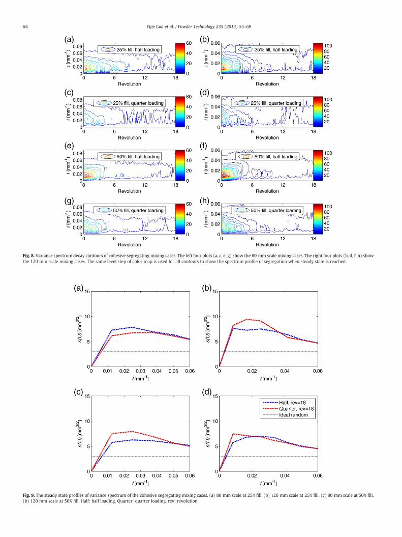
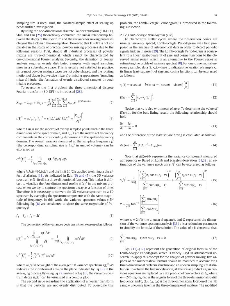
Fig. 8. Variance spectrum decay contours of cohesive segregating mixing cases. The left four plots (a, c, e, g) show the 80 mm scale mixing cases. The right four plots (b, d, f, h) showthe 120 mm scale mixing cases. The same level step of color map is used for all contours to show the spectrum profile of segregation when steady state is reached.

Fig. 9. The steady state profiles of variance spectrum of the cohesive segregating mixing cases. (a) 80 mm scale at 25% fill. (b) 120 mm scale at 25% fill. (c) 80 mm scale at 50% fill.(b) 120 mm scale at 50% fill. Half: half loading. Quarter: quarter loading. rev: revolution.

64 Yijie Gao et al. / Powder Technology 235 (2013) 55–69

65Yijie Gao et al. / Powder Technology 235 (2013) 55–69

0.032]mm−1 for the case of 3.6 cm3 sampling size. In this case, the inte-gration interval covers almost all the main decay components for the120 mm scale mixing, while some components in higher frequency do-mains are missed in the case of the 80 mm scale. This leads to differentfitted RSDdecay curves (Fig. 7b). Therefore, with the principle of similar-ity satisfied, similar variance decay process can be achieved only whenthe sampling size is much smaller than the scale of both mixing geome-tries in the scale-up process.

3.1.2. Cohesive particle mixing caseFig. 8 shows the overall variance spectrum decay contours of co-

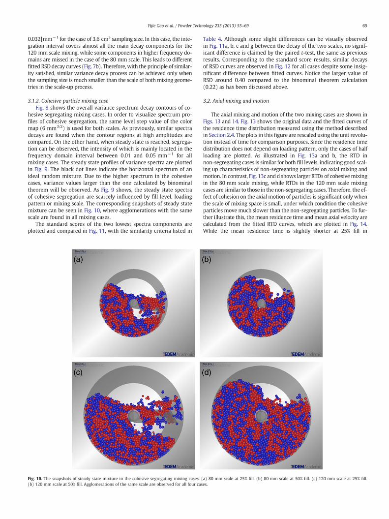
hesive segregating mixing cases. In order to visualize spectrum pro-files of cohesive segregation, the same level step value of the colormap (6 mm3/2) is used for both scales. As previously, similar spectradecays are found when the contour regions at high amplitudes arecompared. On the other hand, when steady state is reached, segrega-tion can be observed, the intensity of which is mainly located in thefrequency domain interval between 0.01 and 0.05 mm−1 for allmixing cases. The steady state profiles of variance spectra are plottedin Fig. 9. The black dot lines indicate the horizontal spectrum of anideal random mixture. Due to the higher spectrum in the cohesivecases, variance values larger than the one calculated by binominaltheorem will be observed. As Fig. 9 shows, the steady state spectraof cohesive segregation are scarcely influenced by fill level, loadingpattern or mixing scale. The corresponding snapshots of steady statemixture can be seen in Fig. 10, where agglomerations with the samescale are found in all mixing cases.

The standard scores of the two lowest spectra components areplotted and compared in Fig. 11, with the similarity criteria listed in

Fig. 10. The snapshots of steady state mixture in the cohesive segregating mixing cases. ((b) 120 mm scale at 50% fill. Agglomerations of the same scale are observed for all four cas

Table 4. Although some slight differences can be visually observedin Fig. 11a, b, c and g between the decay of the two scales, no signif-icant difference is claimed by the paired t-test, the same as previousresults. Corresponding to the standard score results, similar decaysof RSD curves are observed in Fig. 12 for all cases despite some insig-nificant difference between fitted curves. Notice the larger value ofRSD around 0.40 compared to the binominal theorem calculation(0.22) as has been discussed above.

3.2. Axial mixing and motion

The axial mixing and motion of the two mixing cases are shown inFigs. 13 and 14. Fig. 13 shows the original data and the fitted curves ofthe residence time distribution measured using the method describedin Section 2.4. The plots in this figure are rescaled using the unit revolu-tion instead of time for comparison purposes. Since the residence timedistribution does not depend on loading pattern, only the cases of halfloading are plotted. As illustrated in Fig. 13a and b, the RTD innon-segregating cases is similar for both fill levels, indicating good scal-ing up characteristics of non-segregating particles on axial mixing andmotion. In contrast, Fig. 13c and d shows larger RTDs of cohesivemixingin the 80 mm scale mixing, while RTDs in the 120 mm scale mixingcases are similar to those in the non-segregating cases. Therefore, the ef-fect of cohesion on the axial motion of particles is significant only whenthe scale of mixing space is small, under which condition the cohesiveparticles move much slower than the non-segregating particles. To fur-ther illustrate this, themean residence time andmean axial velocity arecalculated from the fitted RTD curves, which are plotted in Fig. 14.While the mean residence time is slightly shorter at 25% fill in

a) 80 mm scale at 25% fill. (b) 80 mm scale at 50% fill. (c) 120 mm scale at 25% fill.es.

Fig. 11. The standard score of spectrum decay curves at the lowest two frequency domains, cohesive segregating mixing cases. (a, c, e, g) f=Δf. (b, d, f, h) f=2Δf. (a, b) 25% fill, halfloading. (c, d) 25% fill, quarter loading. (e, f) 50% fill, half loading. (g, h) 50% fill, quarter loading.

66 Yijie Gao et al. / Powder Technology 235 (2013) 55–69

non-segregating mixing cases, particles stay much longer in 80 mmscale mixing space in the cohesive cases, especially when the lower filllevel is used. It is worth to note that the axial velocity measured in120 mm scale is around 1.5 fold of that in the 80 mm scale due to thescale ratio of mixing space as indicated in Fig. 14c and d.

3.3. Flow rate evaluation

For similar mixing geometries with scale ratio k and constantFroude number the flow rates can be estimated as follows:

r2 ¼ kr1; l2 ¼ kl1 ð31Þ

ω2 ¼ k−0:5ω1: ð32Þ

Since the mean residence time distribution measured by revolu-tion (ωl /vx) is kept the same in the process of scaling up, it followsthat:

vx2 ¼ k0:5vx1: ð33Þ

Table 4Similarity criteria of the standard scores, cohesive segregating mixing cases.

Fill level Loading Frequency h p-Value C.I. (y1–y2) R2

25% Half f=Δf 0 0.9743 −0.0595 0.0615 0.8902f=2Δf 0 0.993 −0.0524 0.0529 0.9168

Quarter f=Δf 0 0.9548 −0.1099 0.1164 0.6142f=2Δf 0 0.8466 −0.0553 0.0673 0.8868

50% Half f=Δf 0 0.9713 −0.0216 0.0224 0.9853f=2Δf 0 0.9743 −0.0211 0.0218 0.9862

Quarter f=Δf 0 0.9493 −0.0670 0.0715 0.8549f=2Δf 0 0.9646 −0.0451 0.0472 0.9356

The scaling relationship of flow rate can then be derived using theformula F=πvxr2 and be expressed as follows:

F2 ¼ k2:5F1: ð34Þ

Therefore, when a four-fold scaling up is applied on the mixing ap-paratus, the flow rate of the larger continuous mixer is 32 fold of theoriginal lab scale apparatus, which indicates a tremendous increase inproduction rate for the continuous powder mixing system. Thisshows the merit of using the model for continuous powder mixingon the scaling up characteristics.

Similar analysis can be performed on the batch mixing systems,where the production rate can be measured as F= l3kb where l3 rep-resents the batch volume and kb the mixing rate described in Eq. (25).Since similar mixing rates, measured by the reciprocal of revolution(kb /ω), are achieved, the scaling relationship of mixing rate isexpressed as

kb2 ¼ k−0:5kb1: ð35Þ

As a result, a scaling up expression of production rate the same asEq. (34) is derived for the case of batch mixing, indicating the inher-ent coincidence of batch and continuous mixing processes.

For the cohesive cases, Eq. (34) can be directly used for the scalingup of batch-like powder mixing process, due to the scaling relation-ship observed in Figs. 8–12. However, larger flow rate will be ob-served in the scaled-up continuous powder mixing process, due to arelatively fast axial velocity in that case. This effect should be consid-ered in the design of scaling up strategy of cohesive mixing cases.

Fig. 12. RSD-t decay curves measured at sampling size of 0.45 cm3, cohesive segregating mixing cases. (a) 25% fill, half loading. (b) 50% fill, quarter loading. (c) 50% fill, half loading.(d) 50% fill, quarter loading.

67Yijie Gao et al. / Powder Technology 235 (2013) 55–69

4. Conclusions

A new methodology based on the concept of variance spectrum hasbeen developed for studying the scale-up of powder mixing in continu-ous processes. The Lomb–Scargle Periodogram technique widely ap-plied in astronomical studies has been used to estimate the variancespectrum of unevenly distributed samples in powder mixing processes.The periodic sectionmodeling, proposed in our previous work [18], per-mits us to consider the batch-like cross-sectional mixing and axial

Fig. 13. Residence time distribution of all mixing cases. (a) Non-segregating cases, 25% fill. (bsegregating cases, 50% fill. rev: revolution.

motion separately for the scale-up of continuous powder mixing pro-cess. Such quantitative investigations are used to clarify the effect of con-stant sampling size on mixing performance, and the effect of scaling upon both cross-sectional and axial mixing within continuous mixing. Forthe non-segregating mixing cases, similar scale-up characteristics areobserved for both cross-sectional and axial mixing in our simulation re-sults.While a satisfying principle of similarity leads to similar decay con-tours of variance spectra, a sampling sizemuch smaller than the scales ofboth apparatuses should be used to achieve similar mixing performance

) Non-segregating cases at 50% fill. (c) Cohesive segregating cases, 25% fill. (d) Cohesive

Fig. 14. The mean residence time and the mean axial velocity of all mixing cases. (a) The mean residence time, non-segregating cases. (b) The mean residence time, cohesive seg-regating cases. (c) The mean axial velocity, non-segregating cases. (b) The mean axial velocity, cohesive segregating cases. rev: revolution.

68 Yijie Gao et al. / Powder Technology 235 (2013) 55–69

measurements. When non-segregating materials are processed, a 2.5fold increase in production rate is obtainable for the scale-up of contin-uous powder mixing. However, in processes where cohesive materialssegregate due to a tendency to agglomerate, an even larger increase offlow rate is expected. This results from the effect of cohesion on axialmotion especiallywhen the scale of themixing process is small. Our pre-liminary simulation results illustrate that the proposed analysis can beused to achieve a successful scale-up strategy for continuous powderblending of large sphere particles. Whether the proposed scaling rela-tionships are applicable to practical systems consisting of small, cohe-sive, and irregular powder requires further investigation.

NomenclatureC concentration (–)E(ti) discrete RTD measurement (s−1)E(t, x) location dependent RTD in continuous blending (s−1)E(ω) sum of square fit (–)f one dimensional spatial frequency (mm−1)f three dimensional spatial frequency (mm−1)fs one dimensional sampling spatial frequency (mm−1)Δf one dimensional minimum detectable spatial frequency

(mm−1)F volumetric flow rate (mm3/s) or cohesive force (N)Fr Froude number (–)g gravity (9.81 m2/s)k scale ratio of blending geometrieskb exponential variance decay rate of batch-like blending (s−1)kc coefficient of cohesion (J·m−3)l scale of geometryPe Peclet number (–)r blender radius (mm)RSD relative standard deviation (–)s(f) one dimensional variance spectrum (mm1/2)s(f) three dimensional variance spectrum (mm3/2)s(f,t) one dimensional variance spectrum decay (mm1/2)s(f,t) three dimensional variance spectrum decay (mm3/2)t time of batch like periodic section blending (s)Δt time interval (s)

tn one dimensional location in Lomb–Scargle Periodogram (mm)tn three dimensional location in Lomb–Scargle Periodogram

(mm)vx axial velocity (mm/s)w(f) weight of averaged one dimensional variance spectrum (–)wn weight of the nth sample in Lomb–Scargle Periodogram (–)x axial location in continuous blender (mm)xn sample as a function of location (–)xf(t) one dimensional fit in Lomb–Scargle PeriodogramX sample in a population (–)Xk one dimensional discrete Fourier transform sample (–)Xh,j,k three dimensional discrete Fourier transform sample (–)Z standard scoreθ dimensionless time (–)or phase lag in Lomb–Scargle

Periodogram (rad)μ mean value of a population (–)ξ dimensionless location (–)σ standard deviation (–)σ2(fs) variance as a function of sample size (–)σ02 initial variance of totally segregated blend (–)

σSS2 steady state variance of random blend (–)

σb2(t) time dependent variance decay curve in periodic section

blending (–)σc2(x) location dependent variance decay curve in continuous

blending (–)τ mean residence time (s) or location lag in Lomb–Scargle

Periodogram (mm)ω angular frequency (rad/mm) or angular velocity of blade

(rad/s)ω three dimensional angular frequency (rad/mm)Ω one dimensional scale of the variance spectrumanalysis (mm)

Acknowledgments

This work is supported by the National Science Foundation Engi-neering Research Center on Structured Organic Particulate Systems,through grant NSF-ECC 0540855, and by grant NSF-0504497.

69Yijie Gao et al. / Powder Technology 235 (2013) 55–69

References

[1] L.T. Fan, S.J. Chen, C.A. Watson, Annual review, Solids Mixing 62 (1970) 53–69.[2] M. Poux, P. Fayolle, J. Bertrand, D. Bridoux, J. Bousquet, Powder mixing: some

practical rules applied to agitated systems, Powder Technology 68 (1991)213–234.

[3] L.T. Fan, Y.-M. Chen, F.S. Lai, Recent developments in solids mixing, PowderTechnology 61 (1990) 255–287.

[4] L. Pernenkil, C.L. Cooney, A review on the continuous blending of powders,Chemical Engineering Science 61 (2006) 720–742.

[5] R.W. Johnstone, M.W. Thring, Pilot Plants, Models and Scale-up Methods inChemical Engineering, MacGraw-Hill, New York, 1957.

[6] R.H. Wang, L.T. Fan, Methods for scaling-up tumbling, Chemical Engineering 81(1974) 88–94.

[7] M. Horio, A. Nonaka, Y. Sawa, I. Muchi, A new similarity rule for fluidized bedscale-up, AIChE Journal 32 (1986) 1466–1482.

[8] A. Alexander, T. Shinbrot, F.J. Muzzio, Scaling surface velocities in rotating cylin-ders as a function of vessel radius, rotation rate, and particle size, Powder Tech-nology 126 (2002) 174–190.

[9] A. Alexander, F. Muzzio, Batch size increase in dry blending and mixing, in: Pharma-ceutical Process Scale-up, Second edition, Informa Healthcare, 2005, pp. 161–180.

[10] A.Z.M. Abouzeid, D.W. Fuerstenau, K.V. Sastry, Transport behavior of particulatesolids in rotary drums: scale-up of residence time distribution using the axial dis-persion model, Powder Technology 27 (1980) 241–250.

[11] E.B. Nauman, Residence time theory, Industrial & Engineering Chemistry Re-search 47 (2008) 3752–3766.

[12] H. Risken, The Fokker–Planck Equation: Methods of Solution and Applications, 2ed. Springer, 1996.

[13] H.E.H. Meijer, P.H.M. Elemans, The Modeling of Continuous Mixers. Part I: TheCorotating Twin‐screw Extruder, in: , 1988, pp. 275–290.

[14] Y.L. Ding, R.N. Forster, J.P.K. Seville, D.J. Parker, Scaling relationships for rotatingdrums, Chemical Engineering Science 56 (2001) 3737–3750.

[15] P.C. Johnson, R. Jackson, Frictional–collisional constitutive relations for granularmaterials, with application to plane shearing, Journal of Fluid Mechanics 176(1987) 67–93.

[16] S.B. Savage, K. Hutter, The motion of a finite mass of granular material down arough incline, Journal of Fluid Mechanics 199 (1989) 177–215.

[17] J.C. Williams, Continuous mixing of solids. A review, Powder Technology 15(1976) 237–243.

[18] Y. Gao, M. Ierapetritou, F. Muzzio, Periodic section modeling of convective contin-uous powder mixing processes, AIChE Journal 58 (2012) 69–78.

[19] P.V. Danckwerts, Continuous flow systems: distribution of residence times,Chemical Engineering Science 2 (1953) 1–13.

[20] J.C. Williams, M.A. Rahman, Prediction of the performance of continuous mixersfor particulate solids using residence time distributions Part I. Theoretical,Powder Technology 5 (1972) 87–92.

[21] K. Marikh, H. Berthiaux, V. Mizonov, E. Barantseva, D. Ponomarev, Flow analysisand Markov chain modelling to quantify the agitation effect in a continuous pow-der mixer, Chemical Engineering Research and Design 84 (2006) 1059–1074.

[22] D. Brone, A. Alexander, F.J. Muzzio, Quantitative characterization of mixing of drypowders in V-blenders, AIChE Journal 44 (1998) 271–278.

[23] O.S. Sudah, A.W. Chester, J.A. Kowalski, J.W. Beeckman, F.J. Muzzio, Quantitativecharacterization of mixing processes in rotary calciners, Powder Technology126 (2002) 166–173.

[24] A. Sarkar, C.R. Wassgren, Simulation of a continuous granular mixer: effect of op-erating conditions on flow and mixing, Chemical Engineering Science 64 (2009)2672–2682.

[25] S.H. Shin, L.T. Fan, Characterization of solids mixtures by the discrete Fouriertransform, Powder Technology 19 (1978) 137–146.

[26] R. Weineköter, L. Reh, Continuous mixing of fine particles, Particle and ParticleSystems Characterization 12 (1995) 46–53.

[27] Y. Gao, F. Muzzio, M. Ierapetritou, Characterization of feeder effects on continuoussolid mixing using Fourier series analysis, AIChE Journal 57 (2011) 1144–1153.

[28] A. Averbuch, Y. Shkolnisky, 3D Fourier based discrete Radon transform, AppliedComputational Harmonic Analysis 15 (2003) 33–69.

[29] R.L. Gilliland, S.L. Baliunas, Objective characterization of stellar activity cycles: I.Methods and solar cycle analyses, Astrophysical Journal (1987) 766–781.

[30] P. Babu, P. Stoica, Spectral analysis of nonuniformly sampled data — a review,Digital Signal Processing 20 (2010) 359–378.

[31] N.R. Lomb, Least-squares frequency analysis of unequally spaced data, Astrophysicsand Space Science 39 (1976) 447–462.

[32] J.D. Scargle, Studies in astronomical time series analysis. II — statistical aspects ofspectral analysis of unevenly spaced data, Astrophysical Journal 263 (1982)835–853.

[33] K. Hocke, N. Kämpfer, Gap filling and noise reduction of unevenly sampled databy means of the Lomb–Scargle periodogram, Atmospheric Chemistry and Physics9 (2009) 4197–4206.

[34] M. Zechmeister, M. Kürster, in: The Generalised Lomb–Scargle Periodogram,2009, pp. 577–584.

[35] D.H.L. Roberts, J., J.W. Dreher, Time series analysis with clean – part one – derivationof a spectrum, Astronomical Journal 93 (1987) 968–989.

[36] G. Foster, The cleanest Fourier spectrum, Astronomical Journal 109 (1995)1889–1902.

[37] P. Stoica, L. Jian, H. Hao, Spectral analysis of nonuniformly sampled data: a newapproach versus the periodogram, IEEE Transactions on Signal Processing 57(2009) 843–858.

[38] T. Shinbrot, A. Alexander, M. Moakher, F.J. Muzzio, Chaotic granular mixing, Chaos9 (1999) 611.

[39] P.E. Arratia, N.-H. Duong, F.J. Muzzio, P. Godbole, S. Reynolds, A study of themixing and segregation mechanisms in the Bohle Tote blender via DEM simula-tions, Powder Technology 164 (2006) 50–57.

[40] P. Portillo, F.J. Muzzio, M.G. Ierapetritou, Hybrid DEM-compartment modeling ap-proach for granular mixing, AIChE Journal 53 (2007) 119–128.

[41] F. Bertrand, L.A. Leclaire, G. Levecque, DEM-based models for the mixing of gran-ular materials, Chemical Engineering Science 60 (2005) 2517–2531.

[42] Y.C. Zhou, A.B. Yu, R.L. Stewart, J. Bridgwater, Microdynamic analysis of the parti-cle flow in a cylindrical bladed mixer, Chemical Engineering Science 59 (2004)1343–1364.

[43] R.D. Mindlin, Compliance of elastic bodies in contact, Journal of Applied Mechanics71 (1949) 259–268.

[44] C. Wightman, F.J. Muzzio, Mixing of granular material in a drum mixer undergo-ing rotational and rocking motions I. Uniform particles, Powder Technology 98(1998) 113–124.

[45] D. Brone, F.J. Muzzio, Enhanced mixing in double-cone blenders, Powder Technol-ogy 110 (2000) 179–189.

[46] Y. Gao, F.J. Muzzio, M.G. Ierapetritou, Optimizing continuous powder mixing pro-cesses using periodic section modeling, Chemical Engineering Science 80 (2012)70–80.

[47] P.M. Portillo, A.U. Vanarase, A. Ingram, J.K. Seville, M.G. Ierapetritou, F.J. Muzzio,Investigation of the effect of impeller rotation rate, powder flow rate, and cohe-sion on powder flow behavior in a continuous blender using PEPT, Chemical En-gineering Science 65 (2010) 5658–5668.

[48] A.U. Vanarase, F.J. Muzzio, Effect of operating conditions and design parametersin a continuous powder mixer, Powder Technology 208 (2011) 26–36.

[49] O.S. Sudah, D. Coffin-Beach, F.J. Muzzio, Quantitative characterization of mixing offree-flowing granular material in tote (bin)-blenders, Powder Technology 126(2002) 191–200.

[50] A.T. Harris, J.F. Davidson, R.B. Thorpe, Particle residence time distributions in cir-culating fluidised beds, Chemical Engineering Science 58 (2003) 2181–2202.

[51] Y. Gao, A. Vanarase, F. Muzzio, M. Ierapetritou, Characterizing continuous powdermixing using residence time distribution, Chemical Engineering Science 66(2011) 417–425.