Session0 Adler1998 - cecas.clemson.educecas.clemson.edu/~cgallag/publications/stable.pdf · c#14(&1), 1)')(,/? #) 0,,(1% $ # a%42 &"#.,. #/ ... .02+4).0/)#(8 * +0#$ 3%)" #48 -

Analysing Stable Time Series

Robert J' Adler+ Raisa E' Feldman+ and Colin Gallagher

Abstract

We describe how to take a stable/ ARMA/ time series through the

various stages of model identi9cation/ parameter estimation/ and diag;

nostic checking/ and accompany the discussion with a goodly number of

large scale simulations that show which methods do and do not work/ and

where some of the pitfalls and problems associated with stable time series

modelling lie=

! Introduction

There are three major stages in the now standard /Box2Jenkins5 time series

modelling techniques for Gaussian time series< Model identi>cation? parameter

estimation? and diagnostic checkingA

In many ways? the techniques behind these three stages really only involve

two bags of tricks? since most diagnostic checks rely on testing whether or not the

>tted residuals? after parameter estimation? behave like a white noise sequenceA

This? of course? is tantamount to identifying a model for the residuals? and so

takes us? more or less? back to stage oneA

In this paper we will concentrate on a variety of issues related to ARMA

model identi>cation in the stable settingA The paper by Calder and Davis? in

this volume? JCDK? describes the parameter estimation problem? so that the two

papers? together? should give a good overview of the overall ARMA problem

and be of some assistance to a practitioner who wishes to analyse a particular

seriesA We shall also have something to say about parameter estimation? for one

speci>c techniqueA

There are no new theorems in this paper? or even really new ways of thinking

about thingsA Rather? we have tried to collect? in one place? a number of results

that are rather widely scattered? and to investigate their practical eMciency on

replicates of synthetic dataA Some of the results are somewhat surprising? and

some more than a little worryingA Many beg further? and deeper? theoretical

investigationA

Research supported in part by O1ce of Naval Research6 grants N8889:;<:;9;89<96 N8889:;

<=;9;8>88 and N8889:;<?;9;8@=<

O

Adler% Feldman and Gallagher

The bottom line will be that while- in principle- the standard Gaussian Box7

Jenkins techniques ;BJ<- ;BD< do carry over to the stable setting- in practice a

great deal of care needs to be exercisedB

Results in a similar vein can also be found in the paper ;R < in this volume-

as well as ;RD< and ;FR<B These papers treat real as well as synthetic data- and

general heavy tailed rather than purely stable seriesB

Finally- before we start- we should determine precisely what we mean by

the various stable parameters by deFning a stable distribution with parameters

G ! "! #! $H as usual via its characteristic functions- as followsI

E eitZ

!J

"exp

# ##jtj# D i"Gsign tH tan $#

!K i$t

$if "J D!

expn #jtj

&D K i%

$ Gsign tH ln jtj'K i$t

oif J D!

GDBDH

where L ) # ! # $ L! D # " # D- and $ % &B We shall denote such a

distribution by writing Z ' S#G#! "! $HB

! Preliminary data analysis . Is it stable1

The Frst question that must be broached is whether or not our data is

Nheavy tailedO- in some general sense- and- if so- whether or not it is stableB We

shall not be interested in the possibility of heavy tailed- but non7stable data-

for a number of reasonsI

DB If the data is in the domain of attraction GcfB ;FE<H of a stable distribution-

then- in general- large sample techniques are identical to those for the

purely stable situationB

B In the domain of attraction case- the diRerence between a stable and non7

stable model lies in the central region of the distributionB If one is using

stable or other heavy tailed techniques- this is generally not the region of

interestB

SB In the case of heavy tails- not in a stable domain of attraction- there are

comparatively few reliable techniques around Gsee ;RD- FR< for further

details and discussionHB

We shall also make one signiFcant simpliFcation throughout this paperI We

shall virtually always work with examples in which- in terms of GDBDH- " J $ J LT

iBeB with centered and symmetric variablesB This simpliFcation is common in

most of the theory that we quote- although- unfortunately- it is not always

justiFed in practiceB However- we doubt that it has much qualitative eRect

on the phenomena we shall look atB That this is deFnitely the case in some

situations is born out by ;KN <B

Analysing stable time series

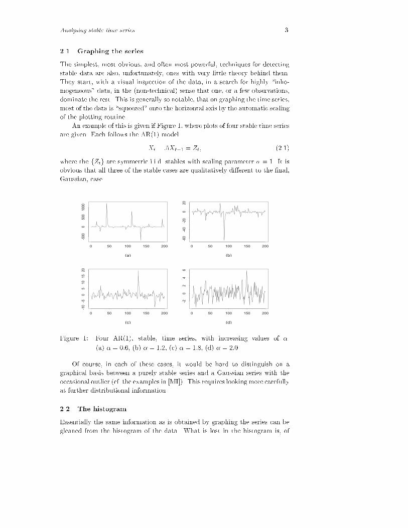
!" Graphing the series!

The simplest* most obvious* and often most powerful* techniques for detecting

stable data are also* unfortunately* ones with very little theory behind them9

They start* with a visual inspection of the data* in a search for highly :inho;

mogeneous< data* in the =non;technical> sense that one* or a few observations*

dominate the rest9 This is generally so notable* that on graphing the time series*

most of the data is :squeezed< onto the horizontal axis by the automatic scaling

of the plotting routine9

An example of this is given if Figure C* where plots of four stable time series

are given9 Each follows the AR=C> model

Xt !FXt G Zt# =H9C>

where the fZtg are symmetric i9i9d9 stables with scaling parameter $ G C9 It is

obvious that all three of the stable cases are qualitatively diJerent to the Knal*

Gaussian* case9

0 50 100 150 200

-500

0500

1000

(a)

0 50 100 150 200

-60

-40

-20

020

(b)

0 50 100 150 200

-10-5

05

1015

20

(c)

0 50 100 150 200

-20

24

6

(d)

Figure CM Four AR=C>* stable* time series* with increasing values of %9

=a> % G N!O* =b> % G C!H* =c> % G C!P* =d> % G H!N

Of course* in each of these cases* it would be hard to distinguish on a

graphical basis between a purely stable series and a Gaussian series with the

occasional outlier =cf9 the examples in RMIT>9 This requires looking more carefully

at further distributional information9

! The histogram!

Essentially the same information as is obtained by graphing the series can be

gleaned from the histogram of the data9 What is lost in the histogram is* of


course' the temporal structure of the data' but what is more obvious is the

presence or absence of symmetry6

Figure 9 shows a histogram from data generated by the same model as in

:96;<' but now only for two cases' = 9 :Gaussian< and = ;!?' and for series

of length ;'@@@6 Two factors should be noted here6 The Brst is that' despite the

fact that the sample size is quite large' the Gaussian case is much further from

the traditional bell curve than one would expect with i6i6d6 data6 But' this is

correlated data' so that the laws of large numbers take longer to come into play6

The second is a repetition of the phenomenon mentioned above' about auH

tomatic scaling IspoilingJ the graph6 In :b< a few outliers are so large that the

entire histogram is squeezed into a few bars in the center6 When the largest

and the smallest MN of the data is truncated' as in :c<' the shape of the graph

changes dramatically6

-4 0 2 4

020

4060

80100

120

(a)-40 0 20 40

0100

200300

(b)-2 0 2

010

2030

4050

(c)

Figure 9O Histograms of :a< Gaussian' :b< Stable' = ;!?' and :c< Truncated

stable time series6

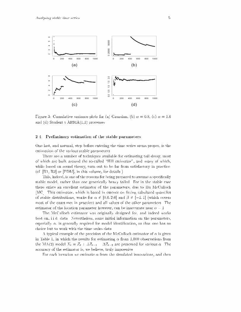
!" The &converging variance/ test!

One of the oldest tests for determining whether data has inBnite variance is the

trick of plotting the sample variance S n' based on the Brst n observations' as a

function of n6 If the data comes from population with Bnite variance' S n should

converge to a Bnite value6 Otherwise' it should diverge as n grows' and the

graph typically shows large jumps6

Although this test was originally designed for i6i6d6 data' it also works well

for correlated data' as long as the order of the observations is Brst randomised'

so as to destroy dependencies that might lead to trends and jumps with other

explanations6

Figure U contains graphs for this test for two stable : = @!V$ ;!?<' GausH

sian' and ItJ :with degrees of freedom< processes6 :By the last we mean an

ARMA process in which the innovations Zt have a Student t distribution6 This

is an interesting case' since it gives a distribution with much heavier than GausH

sian tails' but in the Gaussian domain of attraction6< For variety' we took the

ARMA:;';< model Xt @!UXt ! = Zt Y !MZt !' with series of length ;'@@@6

The divergence of S n' as n grows' and the irregularity of the graphs in the

two stable cases are very marked6


•

••

•

•

••••••••••••••••••••••••••••••••••••••••••••••••••••••••••••••••••••••••••••••••••••••••••••••••••••••••••••••••••••••••••••••••••••••••••••••••••••••••••••••••••••••••••••••••••••••••••••••••••••••••••••••••••••••••••••••••••••••••••••••••••••••••

••••••••••••••••••••••••••••••••••••••••••••••••••••••••••••••••••••••••••••••••••••••••••••••••••••••••••••••••••••••••••••••••••••••••••••••••••••••••••••••••••••••••••••••••••••••••••••••••••••••••••••••••••••••••••••••••••••••••••••••••••••••••••••••••••••••••••••••••••••••••••••••••••••••••••••••••••••••••••••••••••••••••••••••••••••••••••••••••••••••••••••••••••••••••••••••••••••••••••••••••••••••••••••••••••••••••••••••••••••••••••••••••••••••••••••••••••••••••••••••••••••••••••••••••••••••••••••••••••••••••••••••••••••••••••••••••••••••••••••••••••••••••••••••••••••••••••••••••••••••••••••••••••••••••••••••••••••••••••••••••••••••••••••••••••••••••••••••••••••••••••••••••••••••••••••••••••••••••••••••••••••••••••••••••••••••••••

0 200 400 600 800 1000

23

45

6

(a)

•••••••

•••••••••••••••••••••••••••••••••••••••••••••••••••••••••••••••••••••••••••••••••••••••••••••••••••••••••••••••••••••••••••••••••••••••••••••••••••••••••••••••••••••••••••••••••••••••••••••••••••••••••••••••••••••••••••••••••••••••••••••••••••••••••••••••••••••••••••••••••••••••••••••••••••••••••••••••••••••••••••••••••••••••••••••••••••••••••••••••••••••••••••••••••••••••••••••••••••••••••••••••••••••••

•••••••••••••••••••••••••••••••••••••••••••••••••••••••••••••••••••••••••••••••••••••••••••••••••••••••••••••••••••••••••••••••••••••••••••••••••••••••••••••••••••••••••••••••••••••••••••••••••••••••••••••••••••••••••••••••••••••••••••••••••••••••••••••••••••••••••••••••••••••••••••••••••••••••••••••••••••••••••••••••••••••••••••••••••••••••••••••••••••••••••••••••••••••••••••••••••••••••••••••••••••••••••••••••••••••••••••••••••••••••••••••••••••••••••••••••••••••••••••••••••••••••••••••••••••••••••••••••••••••••••••••••••••••••••••••••••••••••••••••••••••••••••••••••••••••••••

0 200 400 600 800 1000

020000

60000

(b)

•••••••••••••••••••••••••••••••••••••••••••••••••••••••••••••••••••••••••••••••••••••••••••••••••••••••••••••••••••••••••••••••••••••••••••••••

•••••••••••••••••••••••••••••••••••••••••••••••••••••••••••••••••••••••••••••••••••••••••••

•••••••••••••••••••••••••••••••••••••••••••••

••••••••••••••••••••••••••••••••••••••••••••••••••••••••••••••••••••••••••••••••••••••••••••••••••••••••••••••••••••••••••••••••••••••••••••••••••••••••••••••••••••••••••••••••••••••••••••••••••••••••••••••••••••••••••••••••••••••••••••••••••••••••••••••••••••••••••••••••••••••••••••••••••••••••••••••••••••••••••••••••••••••••••••••••••••••••••••••••••••••••••••••••••••••••••••••••••••••••••••••••••••••••••••••••••••••••••••••••••••••••••••••••••••••••••••••••••••••••••••••••••••••••••••••••••••••••••••••••••••••••••••••••••••••••••••••••••••••••••••••••••••••••••••••••••••••••••••••••••••••••••••••••••••••••••••••••••••••••••••••••••••••••••••••••••••••••••••••••••••••••••••••••••••••••••••••••••••••••••••••••

0 200 400 600 800 1000

02

46

8

(c)

•

•

•

••••••

•••••••••••••••••••••••••••••••

••••••

•••••••••••••••••••••••••••••••••••••••••••••••••••••••••••••••••••••••••••••••••••••••••••••••••••••••••••••••••••••••••••••••••••••••••••••••••••••••••••••••••••••••••••••••••••••••••••••••••••••••••••••••••••••••••••••••••••••••••••••••••••••••••••••••••••••••••••••••••••••••••••••••••••••••••••••••••••••••••••••••••••••••••••••••••••••••••••••••

••••••••••••••••••••••••••••••••••••••••••••••••••••••••••••••••••••••••••••••••••••••••••••••••••••••••••••••••••••••••••••••••••••••••••••••••••••••••••••••••••••••••••••••••••••••••••••••••••••••••••••••••••••••••••••••••••••••••••••••••••••••••••••••••••••••••••••••••••••••••••••••••••••••••••••••••••••••••••••••••••••••••••••••••••••••••••••••••••••••••••••••••••••••••••••••••••••••••••••••••••••••••••••••••••••••••••••••••••••••••••••••••••••••••••••••••••••••••••••••••••••••••••••••••••••••••••••••••••••••••••••••••••••••••••••••••••••••••••••••••••••••••••••••••••••••••••••••••••••••••••

0 200 400 600 800 1000

0.00.51.01.52.0

(d)

Figure '( Cumulative variance plots for 5a6 Gaussian8 5b6 : ;!<8 5c6 : =!>

and 5d6 Student t ARMA5=8=6 processesD

!" Preliminary estimation of the stable parameters!

One last8 and natural8 step before entering the time series arena proper8 is the

estimation of the various stable parametersD

There are a number of techniques available for estimating tail decay8 most

of which are built around the soKcalled LHill estimatorN8 and many of which8

while based on sound theory8 turn out to be far from satisfactory in practiceD

5cfD OR=8 RPQ or OPDMQ8 in this volume8 for detailsD6

This8 indeed8 is one of the reasons for being prepared to assume a speciTcally

stable model8 rather than one generically heavy tailedD For in the stable case

there exists an excellent estimator of the parameters8 due to Hu McCulloch

OMCQD This estimator8 which is based in essence on Ttting tabulated quantiles

of stable distributions8 works for O;!>" P!;Q and # O!=" =Q 5which covers

most of the cases met in practice6 and all values of the other parametersD The

estimator of the location parameter however8 can be inaccurate near : =D

The McCulloch estimator was originally designed for8 and indeed works

best on8 iDiDdD dataD Nevertheless8 some initial information on the parameters8

especially 8 is generally required for model identiTcation8 so that one has no

choice but to work with the time series dataD

A typical example of the precision of the McCulloch estimator of is given

in Table =8 in which the results for estimating from =8;;; observations from

the MA5P6 model Xt : Zt X ! Zt ! !'Zt ! are presented for various D The

accuracy of the estimator is8 we believe8 truly impressiveD

For each iteration we estimate from the simulated innovations8 and then


from the time series* For the ,nal column2 we estimated the MA parameters

using Whittle:s estimator2 described in Section =2 and computed the residuals*

We then estimated a third time using these residuals2 expecting ?incorrectlyA

that this estimation would be better than from the raw time series* We repeated

this process BC2CCC times* Clearly the estimates obtained from the innovations

are the best2 but2 perhaps rather surprisingly2 McCulloch:s technique seems to

work better when applied to the original time series rather than to the residuals*

Estimation of alpha, MA/01

Innovations Time series Residuals

* C* HH ?C*CHIJA C* K ?C*CJI A C* JI ?C*BCBCA

*L C*LC= ?C*CH HA C*LBB ?C*CKM=A C*LMM ?C*C BJA

B B*CCM ?C*C=HIA B*CCJ ?C*CKIHA B*CB= ?C*C A

B*M B*MCH ?C*CKC A B*MC ?C*C =LA B*MCI ?C*CJM=A

B*= B*=CM ?C*CKLMA B*=CK ?C*C ICA B*=CJ ?C*CJ IA

B* B* C ?C*CJBBA B* CL ?C*CJIBA B* BC ?C*CLLLA

B*L B*LCL ?C*CIHKA B*LBC ?C*CIJJA B*LBM ?C*BCMHA

M B*IKH ?C*C KHA B*IK= ?C*C KIA B*IKM ?C*C LHA

Table BO Mean and standard deviation 1in parentheses4 of 678777 estimates of

alpha using simulated innovation sequence8 corresponding time series and

estimated residuals<

Interestingly2 however2 McCulloch:s estimator does not seem to work as well

for AR processes as it does for pure moving averages2 at least for small values

of 2 the main problem being in the substantially increased sample variance2

rather than in the bias*

There are a number of possible explanations for this2 although we are not

certain which2 if any2 is real* Two candidates for consideration areO

?iA It may simply be due to divergences2 numerical and other2 as becomes

close to the region where the estimator is not supposed to work*

?iiA In the Gaussian case2 the correlation structure is much stronger in the AR?MA

model than in the MA?MA2 and this should aSect estimator variance* Translating

TcorrelationU to TdependenceU in the stable case2 may create a similar problem*

However2 when estimating from the residuals obtained from the Whittle

parameter estimates2 the simulations indicate that the estimates are superior in

the AR case ?at least for BA*

Table M gives the result of a similar study for the model Xt ! "LXt W

"JXt ! X Zt*

Note that these positive results become less than satisfactory when one

leaves the permissible parameter region for the estimator2 and in the region of

X B* We simulated a sample of length BCCC from a of symmetric Cauchy

distribution ? X B$ % X CA and used McCulloch:s estimator to estimate the


location parameter , The mean of 01 of such independent estimates of location

was 67,8 ,

Similarly; estimates of ! for values of ! " 1#7 also give poor and misleading

results, For example; the average of 811 estimates of ! based on independent

samples of 8111 was 0,AB for ! C 1#B; and 1,D0 for ! C 1#0,

Estimation of alpha, AR/01

! Time series Residuals

,7 1,EB7 F1, 8AAG 1, D1 F1,7HBHG

, 1, 0E F1,AD 7G 1, H1 F1,AEAAG

,E 1,EHB F1,81H1G 1,E8E F1,1 1AG

8 8,1BB F1,1DH7G 8,11D F1,1078G

8,A 8,A8B F1,1D 0G 8,A1 F1,10HHG

8,H 8,H1E F1,811 G 8,H10 F1,10EEG

8,7 8,78A F1,81HH 8,71E F1,1 8DG

8,E 8,E8B F1,81 DG 8,E88 F1,1DH8G

A 8,D0H F1,17 1G 8,D0H F1,1700G

Table AI Mean and standard deviation 0in parentheses3 of 567666 estimates of

alpha using simulated time series and estimated residuals9

23 Model Identi8cation

The Jrst step when Jtting data fX % X!% # # # % Xng into a linear ARMAFp% qG

time series model

Xt " ( Xt " # # # " (pXt p C Zt N * Zt N # # #N *qZt q% FB,8G

with i,i,d, innovations fZtg; normal or stable; is the identiJcation of the lag

parameters p and q,

In the Gaussian case model identiJcation techniques are based on analysis

of the sample autocorrelation function FACFG

S+FhG Cn hXt"

XtXt#h-nXt"

X!t % h C 8% A% # # # % FB,AG

or its mean6corrected version;

T+FhG C

n hXt"

FXt " UXGFXt#h " UXG-

nXt"

FXt " UXG!% FB,BG

where UX C n FX N # # # N XnG; and of the equally familiar sample partial

autocorrelation function FPACFG; which; to make some details below easier to

follow; we deJne in detailI


Consider the AR-p. model

Xt " Xt ! ! ! "pXt p 1 Zt$ -234.

5 " z & & & "pzp "1 6$ jzj $ 53 Let Rp 1 8Ri#j 9

pi#j! 1 8(-i j.9pi#j!

be the p % p matrix of ACFs computed under a Bnite variance assumptionD

1 -(-5.$ & & & $ (-p..!$ ! 1 -" $ & & & $ "p.!3 Then the YuleGWalker matrix equation

is

Rp! 1 $ -23K.

and the YuleGWalker estimate of ! is then deBned as solution of

LRpL! 1 L $ -23M.

where LRp 1 8L(-i j.9pi#j! and L 1 -L(-5.$ & & & $ L(-p..!3To deBne the PACF in the AR caseD we consider vectors !"m 1 -"" $ & & & $ "

"m.D

where ""i 1 "i for i $ p and ""i 1 6 when i + p3 For this vector we write YuleG

Walker equation -23K. as Rm!" 1 m$ where m 1 -(-5.$ & & & $ (-m..3 The

PACF at lag mD "mmD is then deBned as the mGth component of the vector

!"m 1 R m 3 SimilarlyD the sample PACF function at lag m$ L"mmD is deBned as

the mGth component of the vector

L!"m 1 LR m L & -23S.

In the heavy tailed case the ACF and PACF do not existD but we can still use

equations -23U. V -23S. to deBne their sample equivalents3

In the general ARMA caseD the PACF at lag h is deBned as the sample

correlation between the residuals of Xt"h and Xt after linear regression -under

a Bnite variance assumption. on Xt" $ Xt"#$ & & & $ Xt"h 3We shall use the notation X"kk for the PACFYs when the centered ACFs X(Ys

of -232. are used in the YuleGWalker equation -23M. instead of the nonGcentered

L(Ys of -23U.3 For most of the simulations we shall prefer to use the centered

variablesD and so will need to assume that . + 53

We shall seeD basically via simulationD that both the ACF and PACF provide

excellent tools for studying stable time series3 It is perhaps rather surprising

that although second moments are inBnite in the stable caseD the tools that

we are used to from the Gaussian case are still availableD albeit with some

modiBcations3

The following subsection sets up the theory underlying the use of the ACF

and PACF3 We then provide some tables for hypothesis testingD followed by

two sections on numerics3 The Bnal subsection looks at the use of the Akaike

Information Criterion in the stable setting3

!" The basic theory!

The theoretical basis for the usage of the sample ACF for the identiBcation of

the order q of a MA-q. time series is the following fundamental result of 8DRU9

-we follow here 8BD9 Theorem 523235.]


Theorem &'( Let fZtg be an iid symmetric sequence of !1stable random vari1

ables and let fXtg be the strictly stationary process6

Xt !

Xj !

#jZt!j $ "#$%&

where Xj !

jjjj#j j" &# for some ' $ "'$ !& % ('$ )*(

De9ne for such a process an analogue of the ACF function6 namely

)"h& !Xj

#j#j!h+Xj

#"j $ h ! )$ +$ ( ( ( ( "#$ &

Then6 for any positive integer h6

"n+ lnn&#$%".)")&& )")&$ ( ( ( $ .)"h&& )"h&&" ' "Y#$ ( ( ( $ Yh&"$ "#$)'&

where

Yk !

Xj #

")"k / j& / )"k & j&& +)"j&)"k&& Sj+S$( "#$))&

Here S$$ S#$ ( ( ( are independent stable variables@ S$ is positive with S$ (S%$""C

!"$%%$" $ )$ '&6 and the Sj ( S%"C

!#$%% $ '$ '& where

C% !

! #!%%&"!%'cos" ! &

if ! )! )

"' if ! ! )(

"#$)+&

The marginal distribution of each Yk is somewhat simpler6 and we have

Yk !

"# X

j #j)"k / j& / )"k & j&& +)"j&)"k&j%

$A#$%

U+V$ "#$)#&

where V and U are independent stable random variables with the same distri1

butions as S$ and S# in ABCDDEC

When ! 3 ) then ABCDGE is also true when .)"h& is replaced by its mean1corrected

version6 5)"h&C

We consider now an example of this theorem in practice$ Let Xt be the

symmetric stable MA"q& processG

Xt ! Zt / 5#Zt!# / * * */ 5qZt!q ( "#$)H&

Then the above theorem implies that

"n+ lnn&#$%"5)"h&& )"h&& '"#) / +

qXj #

j)"j&j%$A#$%

U+V$ h 3 q$ "#$)K&

! Adler% Feldman and Gallagher

where the right hand side reduces to U!V if q 1 !2

Thus one can use the above results to plot con8dence intervals for the ACF

function and identify the parameter q> once the distribution of U!V is known2

A similar result also holds for the distribution of the PACF2 Since B p

and BRpp Rp> the consistency of the YuleDWalker estimates follows2 In fact>

the mean value theorem gives

B!! ! 1 DGB ! H I opGB ! H'

where D is the p " p matrix of partial derivatives of vector function "GzH K1

RpGzH z2 Here RpGzH 1 Mzji jjN

pi#j! ' z" # and ! 1 "G H2 Theorem O2 then

yields that

Gn! lnnH $%GB!! !H$ DGY ' , , , YpH" GO2 PH

where the vector GY ' , , , YpH has distribution described by GO2 H D GO2 OH2

The limiting distribution of the PACFQs is now given by GO2 PH and GO2 H

D GO2 OH> and so is> in general> rather complicated2 However> when p 1 !> the

right hand side of GO2 PH reduces to U!V > which is the same limit as for the ACF

of white noise2 Since in the null hypothesis case this is what is required to test

which of the -mm are zero> we are in the fortunate situation of being able to

use the same distribution twice2

!"# Some important quantiles"

In practice> the distribution of U!V cannot be computed theoretically> but only

via simulation or numerical integration of the joint density of the vector GU' V H

over an appropriate region2

Figure U gives the density of U!V for two values of .2 Note the high tails

of the distribution> which are high even in relation to stable distributions2

Table O contains the WX2YZ quantiles of U!V Gthe distribution of U!V is

symmetricH which for . / [ were found via simulation of Y!!>!!! values of U!V

using a corrected version of the SDplus routine for generating stable random

variables2 Gcf2 MSTN pUO2 The SDplus routine does not quite deliver what you

might expect in the asymetric case\H Our value for . 1 coincides with the

value quoted in MBDN> pYU > and found via numerical integration2


•

•

•

-2 -1 0 1 2

0.0

0.5

1.0

1.5

alpha=1.8alpha=1.5

Figure '( Kernel density estimates of U!V for x 4!5$ 56 and % 7 &8 and &9:

Table =( >?:8@ quantiles of U!V

% >?:8@ quantile % >?:8@ quantile

B:= >:==9eCB' := =:9D8eCBB

B:' ':D58eCB= :' 5:9 'eCBB

B:8 ?:=?8eCB5 :8 5:B8>eCBB

B:D :>9DeCB5 :D :8 DeCBB

B:? ?:?'8eCB :? :B>DeCBB

B:9 =:? BeCB :?8 >:59BeEB

B:> 5:B?5eCB :9 ?:D=?eEB

:B :5'BeCB :> ':?D8eEB

: 9:B99eCBB 5:B :>DBeCBB

:5 8:8=5eCBB

! Estimating the lag parameters via the ACF and PACF!

To see how useful the above results areI and to compare them to an attempt to

estimate the parameters p and q assuming normalityI we conducted the followE

ingI rather illuminatingI double blind study:

We simulated BB time series of length n 7 BBB with symmetric stable inE

novations with % 7 &5: The models were selected at random from the following

Mve models(

Xt 7 Zt$

Xt 7 Zt ! &?Zt $

Xt 7 Zt ! &?Zt C &9Zt !$


Xt !"Xt # Zt#

Xt !"Xt $ !%Xt ! # Zt!

We plotted the ACF and PACF for each of these series9 and then used these

plots to try to identify the true model using the standard time series technique

of looking at the plots and seeing how they behave relative to the CDE conFdence

intervals under a white noise null hypothesisG Since we did not want to assume

$ to be known9 we used conFdence intervals corresponding to the Gaussian

J$ # !K and Cauchy J$ # K casesG JIn fact9 the conFdence intervals for the

true $ # !! and Cauchy cases were indistinguishable to the human eyeG The

Gaussian intervals9 however9 were about !%E shorterGK The conclusions were

then compared against the true modelsG

The procedure showed N E error when Gaussian limits were used and "E

error using Cauchy limitsG Although the error rate clearly depends on experience

of a person doing identiFcation9 it is clear from this study that using stable limits

for heavyPtailed data reduces the error rate signiFcantlyG

!" On asymptotics or /a funny thing happenned on the way to !7!

A fact often touted by stable time series theorists as a compensation for the

diQculties generally associated with stable rather than Gaussian analysis is that

the rate of convergence of R%JhK %JhK to zero is of the order OJTn) lnnU !"K #oJn !#K for all + , $9 which is considerably faster than in Gaussian case when

the rate is on the order of OJn !!KGHowever9 despite this comforting fact9 there are some other9 rather problemP

atic9 phenomena associated with this convergence9 since the rate of convergence

of the distribution of R%JhK %JhK to the limiting distribution is actually very

slowG

Before we mention some theory9 consider Table X9 which indicates how fast

Jor slowK the distribution of R%J K converges to the theoretical one for the white

noise modelG For values of $ # !X# !"# !"D# and !% and sample size n we

computed Y9YYY coeQcients R%J K from independent white noise sequences with

corresponding values of $ and n and checked the percentage of times the coP

eQcient was not within the nominal CDE conFdence intervalG JOf course9 this

should be DEGK For determining conFdence intervals we used three di[erent

distributions\ a stable distribution with the correct $ Jas described aboveK9 a

Cauchy distribution and Gaussian distributionG JiGeG we used either the correct

value of $9 or behaved as if $ # or !KG The results show that when the correct

stable distribution is used9 the convergence to theoretical DE error is very slow9

and that for ]small^ sample sizes of the order of YYY the Cauchy based limits

actually give the best resultsG

The main reason behind this phenomenon seems to be the slow convergence

of the distributions of stable averages to their limiting distributions9 a fact that

has a well documented historyG JcfG TCH9 HA9 HW9 JMU although none of these

quite treats our settingGK

Analysing stable time series !

Table '( Percent error for 012 con3dence interval of 7 8 9: white noise

! n > ??? n > ?:??? n > 1??:??? n > :???:???

8i9 !@stable limits

B' B'! CBCD !B?D !BCE

BE 'B!E 'B1D 'BFD !BFE

BE1 FB1! 1B!1 1B'? 1BF?

BD ?B11 DBF1 EB'' FBC0

8ii9 Cauchy limits

B' BC' FBFC !CBCE '?B ?

BE ?BD? 1BDE F0BDE E!B01

BE1 ?BE? EB 0 E!B?E E0BF1

BD ?BE' 0BE0 EFB?' D?BF0

8iii9 Gaussian limits

B' CB0 CB E ?BD1 ?BD0

BE !B'F !B!F CB ' B!1

BE1 !B1F !BC! CBEC CB1C

BD 'BCC !BFD CB0? CB'

KFrom the practical point of view: this phenomenon shows up in an inter@

esting way in the numericsB Figure 1 shows the values of the upper limits of the

con3dence intervals for 87 8 9 8 99 for various ! and n: based on the limiting

distribution of Theorem and a white noise time seriesB Note how: for PsmallQ

n: the con3dence interval shrinks to a point as !! CB

We are not certain of the reason for thisB One possibility is that for small

n the limiting distribution of U$V is not appropriateB What seems more rea@

sonable: however: is that the norming constants used to obtain the limiting

distribution: while asymptotically correct: are too large 8in an ! dependent

fashion9 for small and intermediate values of nB

It is not totally clear how to get around this problem without using: perhaps:

something like a bootstrapB However: there is growing evidence that in the stable

situation bootstrapping is also problematic 8cfB WLPPRZ in this volumeB9

One possible approach comes out of Table 1: which explores the n > ???

case for di\erent !]sB Our model is again white noise: and we record the per@

centage of times when the sample coe^cient 7 8 9 is outside the 012 con3dence

interval_ iBeB the percentage of wrong identi3cations of the model when the iden@

ti3cation procedure is done by computer and is based on the value of 7 8 9 onlyB

The con3dence levels were computed based on the true !@stable distribution: as

well as Cauchy and Gaussian distributionsB The number of simulations for each

case was m > ?' ???B

It seems that the Gaussian limits perform the most poorly: at least for

! ( )E and that for all ! Cauchy limits not only perform better than the

others: but do quite well on an absolute scaleB 8The error here is never larger


• • ••

•

•

•

•

•

•

•

1.0 1.2 1.4 1.6 1.8 2.0

0.04

0.06

0.08

(a)

•

•

•

•• •

•

•

•

•

•

1.0 1.2 1.4 1.6 1.8 2.0

0.0180.0220.0260.030

(b)

••

•

•

•

•

•• •

•

•

1.0 1.2 1.4 1.6 1.8 2.0

0.0005

0.0015

0.0025

(c)

••

•

•

•

•

•• •

•

•

1.0 1.2 1.4 1.6 1.8 2.0

0.0005

0.0015

(d)

Figure () Con-dence intervals for 67 6 8 6 88 for ! ! ! 9 and various values

of n: 6a8 n ; # <<<= 6b8 n ; (# <<<= 6c8 n ; (<<# <<<= 6d8 n ; # <<<# <<<

than :9@A8: Furthermore= for small ! there is no signi-cant bene-t in using

the con-dence limits based on the true stable distribution: However= for large

!= the rate of the rate of convergence of 7 6 8 to its theoretical distribution is

so slow that Cauchy or Gaussian distribution should be used: Comparison with

Table ! strengthens this point:

Table () Percent error for J(A con-dence interval of 7 6 8# n ; <<<= WN

! true !$stable distribution Cauchy limits Gaussian limits

!" ! # ! # #!"$

! !#" !#% #!$#

!# ! $ !## #!&'

!$ !#( !#$ #!'

!& !&$ !#& #!)

!* !%* ! % $!#'

!' #!** ! ) $!$$

!( &!$( "!%" $!&'

!% "!** "!(& &!##

!) #*!'$ "!&# &!**

#!" &!(" "!(( &!("

In Table ' we continue the theme of using Cauchy based bounds@ regardless

of the true value of ! While this clearly gives a conservative test@ it turns

out that in practice it is not overly so@ and the results here illustrate how

amazingly well the Cauchy bounds perform in the identiFcation of the MAI J


model Xt ' Zt "(Zt ) Again/ each speci4c case was runm ' 8$ 888 times) In

each run for sample size n ' 888 and given & we computed >'? @$ " " " $ >'? 8@ and

recorded an AerrorB when >'? @ was within the con4dence limits for white noise or

when >'? @ was outside these limits but one of the coeDcients >'?E@$ " " " $ >'? 8@ was

also outside the limits/ so identi4cation as MA? @ would not be called for) The

con4dence limits were taken to be ?i@ ?ln n(n@ !"?U(V @ with U and V coming

from the true distribution/ ?ii@ as in ?i@ but with U and V corresponding to

Cauchy distribution and with & ' / ?iii@ "KL(pn/ ?iv@ according to BartlettNs

formula for MA? @ model with true value of '? @) The whole procedure was

performed by computer without human intervention)

It is clear/ although perhaps somewhat surprising/ that Cauchy limits work

the best and that the identi4cation procedure works better for heavyOtailed

series than for their 4nite variance counterparts)

Table LP Percent of wrong identi4cations of MA? @ model

& true &$stable Cauchy Gaussian Bartlett

)8 8)R 8)R S)RL E)KS

) )L E) R E8)RL T)(

)E )T( E)8( EE) ! !)R(

)R E)KL E)TT E!) 8 L)LT

)T T)(K E)!R ES)S! S)(8

)! E8)RR R)(8 R )KK K)S

)L E() K R)L8 R!)!E E8)(8

)S T!)!K R)!8 T8)RR EE)RE

)( L()!! R)(! TR)TK ER)K!

)K K )!K T)(L T()RK EL) S

E)8 !E)!K S)E !E)!K EK)SR

We close this subsection with a some brief information on the asymptotic

behaviour of the PACF/ which/ not surprisingly/ is similar to that of the ACF)

Table S is a PACF version of Table !/ generated in the same fashion/ however

with data on >+ rather than >'? @ being tabulated)


Table '( Percent error for 012 con3dence interval of 7 ! n 8 999: WN

# true #$stable distribution Cauchy limits Gaussian limits

=9 =9' =9' =0>

= =?' =>9 ?=>0

=? = > =?1 ?=@@

=> =@> =>! ?=!?

=@ =@@ =?9 >=

=1 =A' =>9 >=?>

=! ?=@1 =9A >=>>

=' @=!@ 9=A@ >=A!

=A 9=1? 9='9 @=>1

=0 ?1=0> 9=@' @= >

?=9 @=A@ 9=A> @=A@

!" The AIC criterion!

In the 3nite variance case the prime criterion for automated model selection

recommended by IBDL is the AICC: a modi3ed version of AkaikePs AIC criteQ

rion= An investigation of the AIC criterion in the in3nite variance situation was

carried out by IBHL and IKN L=

For an autoregressive model the AIC statistics are de3ned by

AICWkX 8 n ln Y(!WkX Z ?k!

where n is the sample size: and Y(!WkX is the estimate of the innovation variance

obtained from YuleQWalker estimates for kQth order autoregressive sequence Wcf=

W>=!XX= Then

Yp 8 argmink KAICWkX!

where K is an acceptable upper bound for p: is the corresponding estimate of

the order p= IKN L showed that this procedure is consistent for heavy tailed

situations=

To see how the AIC criterion works in practice for stable AR series we

performed 999 simulations of the ARW X model

Xt 8 9,@Xt! Z Zt! W>= 'X

for # 8 9,1! ,9! ,'1! ?,9= The sample size was 3xed at n 8 ?99: which is rather

small by stable standards: where larger sample sizes are required than in the

Gaussian case=

In each run we assumed that we were looking for the best AR modela i=e=

we looked for order p which minimised the AIC criterion= We then recorded the

number of times that the correct order Wp 8 X was correctly identi3ed=

To check how the AIC criterion works for a MA model: we used the SQplus

arima3mle routine which de3nes AIC as W ?X times the log Gaussian likelihood


plus two times the number of parameters 2t 3see the de2nition in 5BD89 p: ;<=

or consult the S@plus manualA: We performed <<< runs for modelC

Xt D Zt E <"FZt 3;: FA

with # D <"G$ "<$ "!G$ H"<9 n D H<<: Again9 in each run we assumed that

we were looking for the best MA model9 and recorded the number of correct

identi2cations: The results of simulations for both models are given in Table

F and the conclusion is that in both cases the AIC criterion works better the

heavier the tailsQ

The MA case is particularly interesting9 since we have no theoretical justi@

2cation for applying the AIC based on the Gaussian likelihood to heavy@tailed

data:

! Parameter estimation for ARMA models2 The Whittle estimator!

Paper 5CD8 of this volume gives an extensive review of estimation techniques

for linear processes with stable innovations: They present convincing evidence

to the eXect that LAD and MLE estimators are superior9 in the heavy tailed

setting9 to the estimators traditionally used in 2nite variance time series9 such

as least square or Whittle 3periodogramA estimators: However9 for both of these

cases9 the sampling distribution of the parameter estimates is9 at least at the

moment9 numerically as well as theoretically intractable:

Table FC Percent of correct model identi2cations made by AIC:

# AR"#$ % "&'#($ MA"#$ % "&'#*$

<:G \]: \H:G

:< F\:] F\:<

:!G !F:! !\:!

H:< !;:H !H:G

However9 for the Whittle estimator9 we have the following result of 5MGKA8C

Theorem !6 Let fXtg be a causal4 invertible4 #9stable4 ARMA"p$ q$ process4with parameters ( D 3) $ " " " $ )p$ * $ " " " $ *qA!' Let C denote the space of per9

missable parameter valuesA i'e' C D f( " #p!q C )3zA $ *3zA %D < for jzj ' and

)3$A$ *3$A have no common zeroesg' DeDne the polynomials

)3zA D ( ) z ( " " "( )pzp$ *3zA D E * z E " " "E *qzq 3=: A

and4 for all (- . / ' -4 the Fpower transfer functionG

g3/_(A D

*3e i$A "

j)3e i$Aj"" 3=:HA


Denote the self)normalized periodogram by

In!X "!# $

Pnt !Xte

i%t "Pnt !X

"t

$ % & ! ! %' "%&'#

The periodogram5 or 6Whittle8 estimator ((n of the true5 but unknown5 parameter

(#5 is found by minimizing

)"n"(# $)%

n

Xj

In!X"!j#

g"!j *(#"%&%#

with respect to ( " C$ where the sum is taken over all frequencies !j $ )%j.n "" %$ %+' Then5

# n

lnn

$ !'( %((n (#

&# %%W !"(##

S#

!Xk !

Skbk$ "%&.#

where the S#$ S!$ ' ' ' are as in Theorem ?5 W !"(## is the inverse of the matrix

W "(## $Z *

*

(2ln g"!*(##

2(

)(2ln g"!*(##

2(

)Td!$

and

bk $

)%

Z *

*e ik%g"!*(##

2g !"!*(##2(

d!$

where g ! denotes the reciprocal of gA

Self2normalization of the periodogram> as in "%&'#> is essential for the proof

of the above Theorem& However> in practice> in order to Fnd the estimator((n we minimize expression "%&%# when self2normalized periodogram In!X "!# is

replaced by

IIn!X"!# $

n !'(nXt !

Xte i%t

"

"%&J#

One of the useful aspects of this result is that the asymptotic sample dis2

tribution involved here is closely related to that which arises in the study of

the ACF and PACF> so that simple extensions of the numerics required to Fnd

conFdence intervals there also work here&

To see how close the theoretical asymptotic distribution of Whittle estima2

tor is to the true sample distribution when n is Fxed> we simulated data using

the AR" # model "'& U#& We ran three diVerent sample sizes n $ )WW$ WWW

and W$ WWW and two values of 5 $ '.$ 'U.& For comparison we also simulated

Gaussian data and used conFdence intervals for the MLE> the asymptotic dis2

tribution of which coincides with the distribution of Whittle estimates in the

Fnite variance case& We ran m $ W$ WWW simulations for each particular case&

The results> described in Table \ and on Figure J> show that the conFdence

intervals based on the limiting distribution "%&.# work very well even for the


relatively small sample size of n 0 1223 The entries in Table ! are the percent

of estimates 9!n f9" gn which fall into the !;< con=dence interval centered

around the true parameter value3 AlthoughB the numbers in the Gaussian row

are the closest to theoretical !;<B the results for # 0 $D; are impressive and

unexpectedB given the slow convergence rate of the distributions of the sample

ACF and PACF3 Figure I gives histograms for the Whittle estimate f9" gn for

# 0 $D; and the three diKerent sample sizes used3 The vertical bars represent

!;< con=dence levels3

Table !L Percent of f9" gnMs within !;< con=dence intervalN model OP3 DQ

# sample size n)*++ sample size n),+++ sample size n),++++

3; !!3P; !R3SR !I3S

3D; !13D !P3DI !;32R

1 !S3DD !S3;; !S3R!

0.2 0.4 0.6

0500

1000

(a)0.2 0.4 0.6

0100

0200

0300

0

(b)0.30 0.35 0.40 0.45 0.50

0100

0200

0300

0400

0

(c)

Figure IL Histograms and theoretical !;< con=dence intervals for Whittle estiU

mate f9" gn of " in model OP3 DQB OaQ n 0 122B ObQ n 0 222B OcQ n 0 2% 2223

! Diagnostic checking

After identifying and estimating the parameters of times series modelB it is

always nice Oalthough sometimes disconcertingQ to see if the estimated model

is really a good =t to the data3 This is where diagnostic checking procedures

come in3 This usually involves identifying the residuals and seeing how well

they match the distribution originally assumed for the innovations3 In our caseB

this involves checking whether the residuals are i3i3d3 under the assumption of

an S#S distribution3

For in=nite variance series we recommend the four following stepsL

OiQ Graph the residualsN the pattern should follow a white noise model3

OiiQ Check that the ACF and PACF of the residuals are those of white noise3

The results and recommendations of Section P all apply here3

OiiiQ The DurbinUWatson test of ZPL\N

OivQ Various nonUparametric testsB see ZBD\B p3P 1UP P3

We ran a small simulation to see how well the second of these techniques acU

tually worked3 For models OP3 DQ and OP3 RQB stable parameters # 0 $;% $D;% 1B


and sample sizes n , !!! -!!!! -!! !!! we simulated data1 identi2ed a model

using the techniques of Section :1 estimated parameters <using the Whittle es>

timator? and then checked whether the residuals were consistent with stable

white noise modelB

Table -!D Diagnostic checking based on ACFIPACFK models <:B-L?M<:B-N?

Model n Ident( O"n Diag( Check 1C2 Diag( Check1G2

# , -$P

<:B-L? !! AR<-? <C? B:PP WN NOT WN

<:B-N? !! MA<-? <C? BNUL WN NOT WN

<:B-L? -!!! AR<-?<C?! B:NN WN WN

<:B-N? -!!! MA<-? <C? BLNP WN WN

<:B-L? -!!!! AR<-? <G? BW! NIA WN

<:B-N? -!!!! MA<-? <G? BLX: NIA WN

# , -$LP

<:B-L? !! AR<-? <C? B:NN WN WN

<:B-N? !! MA<-? <C?" BN:P WN NOT WN

<:B-L? -!!! AR<-? <C? BW!! WN WN

<:B-N? -!!! MA<-? <C?# BN ! WN NOT WN

<:B-L? -!!!! AR<-? <G? BW!W NIA WN

<:B-N? -!!!! MA<-? <G? BLXL NIA NOT WN

# , $!!

<:B-L? !! AR<-? <G? BWW: WN WN

<:B-N? !! MA<-? <C?$ BLUL WN WN

<:B-L? -!!! AR<-? <G? B:XN WN WN

<:B-N? -!!! MA<-? <C? BN WN WN

<:B-L? -!!!! AR<-? <G? BW P NIA NOT WN

<:B-N? -!!!! MA<-? <G? BN!- NIA WN

Gaussian and true -$P7stable limits indicate MA1;;2( AIC indicates MA1;2(! Cauchy limits indicate AR1;2 or ARMA1;>;2( AIC indicates AR1;2(" Gaussian and true -$LP7stable limits indicate MA1?2( AIC indicates MA1;2(# Gaussian limits indicate MA1?2( True -$LP7stable limits indicate possibly

MA1B2( AIC indicates MA1;2 or MA1?21the value is almost the same2( For

reasons of parsimony we chose MA1;2($ True Gaussian limits indicate MA1;G2> while Cauchy limits indicate correctmodel MA1;2( AIC indicates MA1;2(

Model identi2cation was based on ACFIPACF analysis1 unless more than

one model seemed acceptable1 in which case we diZerentiated between the mod>

els via the AICB For the ]small^ sample sizes of n , !!! -!!! we used Cauchy

based con2dence limits for the ACFIPACF analysis1 while for n , -!! !!! we

used Gaussian limitsB In 2tting the residuals1 with sample sizes n , !!! -!!!


we used both Cauchy and Gaussian limits4

The results summarized in Table !8 show that diagnostic checking based

on ACF=PACF works as well in stable case as in the Gaussian4 The letters

?C@ or ?G@ in the table indicate thatA respectivelyA Cauchy or Gaussian based

conDdence limits were used4 The coeEcient estimate F n is G! in the AR?!@

?I4!J@ caseA and G" in the MA?!@ ?I4!L@ case4

As a guide to reading the tableA consider the Drst lineA which indicates

that an AR?!@ series of length n N 88 and stable innovations with $ N !%O was

generated according to the model ?I4!J@4 It was correctly identiDed as an AR?!@

modelA using Cauchy conDdence intervals for the ACF and PACF4 The estimate

of the the AR coeEcient was 4IOO4 ?The actual value was 84QR cf4 ?I4!J@4@ The

residuals were then investigated4 Using Cauchy conDdence intervals they were

judged to be whiteA which was not the case with Gaussian conDdence intervals4

Although we have not studied itA we note that a stable analogue of the

DurbinVWatson statistic has been developed in XPLZ4 Since this statistic essenV

tially checks that the ACF of the residual sequence at lag ! is that of white

noiseA its asymptotic distribution is given by Theorem I4!4

Unfortunately no otherA strongerA tools ?such as the &! test in the Dnite

variance case@ are currently available for diagnostic checking in the stable situV

ation4 This would seem to be a promising and important direction for further

research4

! Acknowledgement

We are grateful to Dr4 Aaron Gross who wrote the initial SVPlus programs

that this study was based on4

Appendix1 McCulloch6s quantile estimator of stable parameters

In this section we describe the estimator developed by McCulloch ?XMCZ@

for the indices $ ?of stability@ and ?of skewness@ of a stable distributionA which

have been referred to in the body of the paper4

Let X S!?)* * +@ and denote the pVth quantile of this distribution by

Xp4 McCulloch]s estimator uses Dve quantiles to estimate $ ! X8%^* %8Z and

! X"!* !ZA and is structured as follows_

Set

` ?$* @ NX#"# "X#$#X#%# "X#!#

*

`!?$* @ NX#"# aX#$# " X##$

X#"# "X#$#%

Since ` is monotonic in $ and `! is monotonic in ?for Dxed $@ we can we


can invert these functions to obtain

/ 0 12 !2!3!

" / 0!12 !2!3#

McCulloch tabulated 0 and 0! for various values of 2 and 2!8To form an estimator; take a random sample from a stable distribution

and de>ne ?2 and ?2! by replacing the quantiles Xk by the corresponding samC

ple quantiles ?Xk8 Since the sample quantiles are consistent for the population

quantiles; ?2 and ?2! are consistent estimators of 2 and 2!8 De>ne

? / 0 1?2 ! ?2!3!

?" / 0!1?2 ! ?2!3#

Given a random sample from a stable distribution; we can now use the tables

to >nd ? and ?"8

To obtain estimates of the scale and location parameters; McCulloch de>ned

similar functions using these same H quantiles; which were also tabulated for

various scale and location values8 These tables can be used in a similar fashion

so as to obtain estimates for % and for &8

References

IBJL G8 E8 P8 Box and G8 M8 Jenkins Time Series Analysis, Forecasting and

Control Wiley; New York; STUV8

IBDL P8 J8 Brockwell and R8 A8 Davis; Time Series, Theory and Methods;

Springer; New York; STTS8

IBHL R8 Bhansali; Consistent order determination for processes with in>nite

variance; J7 R7 Statist7 Soc7 B; Vol8 H[ 1ST\\3; ]V^V[8

ICDL M8 Calder and R8 A8 Davis; Inference for linear processes with stable

noise; this volume8

ICHL G8 Christoph; On some diaerences in limit theorems with a normal or

a nonCnormal stable limit law; Math7 Nachr7; Vol8 SHb 1STTS3; ]U^ HV

ICMSL J8 M8 Chambers; C8 L8 Mallows and B8 W8 Stuck; A method for simC

ulating stable random variables; Journal of the American Statistical

Association; Vol8 US 1STUV3; b][^b]]8

IDRSL R8 A8 Davis and S8 Resnick; Limit theory for moving averages of random

variables with regularly varying tail probabilities; Ann7 Prob7; Vol8 Sb

1ST\H3; SUT^STH8


"DR % R& A& Davis and S& Resnick2 Limit theory for the sample covariance and

correlation functions of moving averages2 Ann" Statist"2 Vol& @A B@CDEF2

G!!HGGD&

"FE% W& Feller2 An Introduction to Probability Theory and Its Applications2

Vol& II2 Ath ed&2 Wiley2 New York2 @CD!&

"FR% P& D& Feigin and S& R& Resnick2 Pitfalls of Qtting autoregressive models

for heavyRtailed time series2 in preparation&

"HA% P& Hall2 TwoRsided bounds on the rate of convergence to a stable law2

Z" Wahrsch" verw" Gebiete2 Vol& GV B@CD@F2 !ACH!EA&

"HW% L& Heinrich and Wr& Wolf2 On the convergence of U Rstatistics with

stable limit distribution J" Mult" An"2 Vol& AA B@CC!F2 EEH VD

"JM% A& Janssen and D& M& Mason2 On the rate of convergence of sums of

extremes to a stable law2 Probab" Theory and Rel" Fields2 Vol& DE B@CC[F2

G!H EA&

"KN@% K& Knight2 Consistency of Akaike^s information criterion for inQnite

variance autoregressive processes2 Ann" Statist"2 Vol& @V B@CDCF2 D AH

DA[&

"KN % K& Knight2 Rate of convergence of centred estimates of autoregressive

parameters for inQnite variance autoregressions2 J" Time Ser" Anal"2

Vol& D B@CDVF2 G@HE[&

"LPPR% R& LePage2 K& Podg_orski2M& Ryznar2 Bootstrapping signs and permuR

tations for regression with heavy tailed errorsb a seamless resampling2

this volume&

"MC% J&H& McCulloch2 Simple consistent estimators of stable distribution paR

rameters2 Communications in Statistics A Computation and Simulation2

Vol& @G B@CDEF2 @@[CH@@!E&

"MGKA% T& Mikosch2 T& Gadrich2 C& Klduppelberg and R&J& Adler2 Parameter

estimation for ARMA models with inQnite variance innovations2 Annals

of Statistics Vol& ! B@CCGF2 ![GR! E&

"MI% T& Mikosch2 Periodogram estimates from heavy tailed data2 this volR

ume&

"NS% C& L& Nikias and M& Shao2 Signal Processing with AlphaDStable DistriD

butions and Applications2 Wiley2 New York2 @CCG&

"PDM% O& V& Pictet2 M& M& Dacorogna2 U& A& Mduller2 Behaviour of tail estiR

mates under various distributions2 this volume&


"PL% P& C& B& Phillips. and M& Loretan. The Durbin;Watson ratio under

in=nite;variance errors. J! of Econometrics. Vol& !A BCDDCE. FGHCC!&

"RC% S& Resnick. Heavy tail modelling and teletraPc data. Ann! Statistics.

CDDA&

"R % S& Resnick. Why non;linearities can ruin the heavy tailed modellerQs

day. this volume&

"ST% G& Samorodnitsky. and M& Taqqu. Stable Non6Gaussian Random Pro6

cesses. Chapman;Hall. New York. CDD!&

Robert J& Adler Raisa E& Feldman and Colin Gallagher

Department of Statistics Statistics and Applied Probability

UNC Chapel Hill UC Santa Barbara

Chapel Hill. NC. AGDD;] ^_ Santa Barbara. CA. D]C_^; _G_

and

Faculty of Industrial Engineering

Technion. Haifa. ] ___. Israel&

adlerastat&unc&edu epsteinapstat&ucsb&edu

radleraie&technion&ac&il colinapstat&ucsb&edu

Documents

Session0 Adler1998 - cecas.clemson.educecas.clemson.edu/~cgallag/publications/stable.pdf · c#14(&1)*, 1)')(,/? #)* 0,*,(1% $ # a%4*2 &"#.,. #/ ... .02+4).0/)#(8 * +0#$ 3%)" #48 -

Session0 Adler1998 - cecas.clemson.educecas.clemson.edu/~cgallag/publications/stable.pdf · c#14(&1), 1)')(,/? #) 0,,(1% $ # a%42 &"#.,. #/ ... .02+4).0/)#(8 * +0#$ 3%)" #48 -