sensors

Article

Eddy Current Testing with Giant Magnetoresistance(GMR) Sensors and a Pipe-Encircling Excitation forEvaluation of Corrosion under Insulation

Joseph Bailey *, Nicholas Long ID and Arvid Hunze *

Robinson Research Institute, Victoria University of Wellington, Lower Hutt 5010, New Zealand;

Nick.Long@vuw.ac.nz

* Correspondence: joseph.bailey@vuw.ac.nz (J.B.); arvid.hunze@vuw.ac.nz (A.H.);

Tel.: +64-4-463-0095 (J.B.); +64-4-463-0076 (A.H.)

Received: 18 August 2017; Accepted: 26 September 2017; Published: 28 September 2017

Abstract: This work investigates an eddy current-based non-destructive testing (NDT) method to

characterize corrosion of pipes under thermal insulation, one of the leading failure mechanisms for

insulated pipe infrastructure. Artificial defects were machined into the pipe surface to simulate the

effect of corrosion wall loss. We show that by using a giant magnetoresistance (GMR) sensor array and

a high current (300 A), single sinusoidal low frequency (5–200 Hz) pipe-encircling excitation scheme it

is possible to quantify wall loss defects without removing the insulation or weather shield. An analysis

of the magnetic field distribution and induced currents was undertaken using the finite element

method (FEM) and analytical calculations. Simple algorithms to remove spurious measured field

variations not associated with defects were developed and applied. The influence of an aluminium

weather shield with discontinuities and dents was ascertained and found to be small for excitation

frequency values below 40 Hz. The signal dependence on the defect dimensions was analysed in

detail. The excitation frequency at which the maximum field amplitude change occurred increased

linearly with the depth of the defect by about 3 Hz/mm defect depth. The change in magnetic

field amplitude due to defects for sensors aligned in the azimuthal and radial directions were

measured and found to be linearly dependent on the defect volume between 4400–30,800 mm3 with

1.2 × 10−3−1.6 × 10−3

µT/mm3. The results show that our approach is well suited for measuring

wall loss defects similar to the defects from corrosion under insulation.

Keywords: eddy current testing; giant magnetoresistance (GMR) sensor; magnetic field analysis;

corrosion under insulation; pipeline

1. Introduction

Detection of the corrosion of pipe infrastructure is an important area of applied research.

The annual maintenance-related expenses for the petroleum-refining industry in the USA alone

is estimated to be $1.8 billion USD [1]. Usually, the equipment in processing and refinery plants is

operated at elevated temperatures, so that it is necessary to insulate the pipe with a thermal insulation

layer and weather shield. Corrosion under insulation (CUI) refers to corrosion on the external surface

of piping and vessels underneath the insulation layer, and is one of the leading failure mechanisms

for insulated pipe infrastructure. Breaks in the weather shield can lead to the ingress of water, which

in combination with (cycling) processing heat leads to corrosion at the pipe surface [2]. According to

an Exxon Shell study, the highest incidence of leaks in the refining and chemical industries is due to

CUI and adds up to about 10% to total plant maintenance costs [3]. The consequences of not inspecting

for corrosion can be catastrophic, since a pipe can rupture, which usually results in the complete

shutdown of a plant or process for an extended period [4].

Sensors 2017, 17, 2229; doi:10.3390/s17102229 www.mdpi.com/journal/sensors

Mor

e in

fo a

bout

this

art

icle

: ht

tp://

ww

w.n

dt.n

et/?

id=

2172

7

Sensors 2017, 17, 2229 2 of 21

The simplest and most widely used inspection method is the visual inspection of the pipe surface,

but this is costly as it requires the complete removal of insulation and weather shield, which also

has to be reinstated after inspection. A shutdown may also be necessary if the plant cannot operate

with uninsulated pipes. A tool that enables the screening of pipes without removing the insulation is,

therefore, beneficial to the industry.

Radiography has been demonstrated as a fast method that allows the characterization of

small defects and deposits. Its disadvantages are: only a small area can be surveyed; a complex

three-dimensional geometry of source and detectors is required; access from at least one side of the

pipe is needed; and strict safety requirements apply [5]. Successfully demonstrated techniques include

backscatter X-ray [6], gamma ray [7], backscatter gamma ray [8,9], tangential radiography [10] and

computer tomography [11].

Ultrasonic guided-wave inspection of pipes offers the possibility of rapid screening of long lengths

of pipework for corrosion and other defects [12–14], with a typical test length being in the order of

50 m. Although only a small access area is needed, parts of the insulation have to be removed and

good coupling between the transducer array and the pipe has to be guaranteed [15]. The technique

needs a very good calibration procedure and is limited in its capability to determine the exact amount

and location of wall loss [16]. Furthermore, it is complex to use for non-straight pipe sections [17].

A variant of ultrasonic testing uses an electromagnetic pulse instead of an acoustic pulse to

generate an elastic wave that can be analysed via a second encircling coil. This technique allows

evaluation without the need for a couplant. It also enables a substantial lift-off, but the technique has

only been demonstrated in an experimental laboratory setup [18].

Other methods such as neutron backscatter [19] and microwave [20] work indirectly by using

radiation to detect excess water and indicate potential CUI hot-spots. They are quick and accurate

methods for characterizing areas susceptible to CUI and do not require the removal of insulation.

Their disadvantage is that they only register smaller areas where water has accumulated under the

insulation, rather than directly measuring the amount of corrosion.

Based on rerouting of directly injected currents, another recently demonstrated method injects

a current into the pipe itself and measures the magnetic field change from the rerouted currents due to

a defect. It has the advantage of not requiring a complex excitation scheme, but the disadvantage that

the insulation has to be removed at the injection point [21].

Eddy current testing is a well-known and accepted technique for non-destructive testing and

has been used to identify cracking, pitting and corrosion in metallic infrastructure [22]. By passing

an alternating current through an excitation system, eddy currents are induced in the device being

tested. Variations in the electrical conductivity and magnetic permeability, especially the presence

of defects, cause a change in the eddy current induced and the current flow, and thus a change in

phase and amplitude of the corresponding magnetic field. By using a low excitation frequency it is

possible to measure through a conductive weather shield and enable the exciting field to penetrate the

pipe well.

An advantage of eddy current testing is that it is a non-contact method with potentially a large

stand-off distance that does not require surface preparation. A disadvantage is that changes in

pipe lift-off, pipe permeability variations or discontinuities such as pipe bends or protrusions,

can overshadow the defect signals or generate false positives [23].

Eddy current testing in its most basic form detects the change in magnetic field by measuring the

impedance change in the excitation system itself.

Measuring the magnetic field via a magnetic sensor (array) gives spatial information that leads to

better defect identification and quantification.

Giant magnetoresistance (GMR) sensors have a very low 1/f noise [24], which maximises the

signal-to-noise ratio and enables the use of a low excitation frequency. Furthermore, due to their small

size and low power consumption these solid-state thin-film magnetic sensors also allow the fabrication

of compact sensor arrays enabling high spatial resolution scanning.

Sensors 2017, 17, 2229 3 of 21

GMR sensors are now widely adopted for eddy current non-destructive testing (NDT) [25,26]

and used for detection of small cracks [27] and subsurface cracks in aircraft structures [28], rebars in

concrete [29], PCB boards [30] or support structures in steel bridges [31].

GMR sensors are also used to detect defects and corrosion in pipes. GMR sensor arrays were

successfully implemented to detect cracks and defects in pipes in the pipe production process using

magnetic flux leakage excitation and sensors close to the pipe surface [32–34]. A system based on

a rotating magnetic field excitation scheme in combination with 6 GMR sensors inside a 70 mm diameter

pipe with very small lift-off was able to detect defects down to 1.5 × 13.5 × 5 mm3 volume [35].

Another approach uses GMR sensors in combination with a meandering wire excitation scheme,

targeting corrosion under insulation. It can detect corrosion patches as small as 38 × 38 × 3 mm3,

under 50.8 mm insulation including a 0.5 mm thick aluminium weather shield [36,37].

A different form of eddy current-based technique uses pulsed eddy currents (PEC) [38–40].

This technique is based on the transient eddy currents following a sharp electromagnetic transition.

Apart from being able to be used with a thick insulation and weather shield, the accuracy of PEC is

good and it allows remaining wall thickness to be estimated. The disadvantage is that PEC averages

the signal over a larger area, with dimensions typically in the range of twice the insulation thickness.

Therefore, defect sizing is complex and it may miss small localised defects [38]. A pipe-encircling

excitation system, similar to our approach, with a lift-off of 50 mm and 4 GMR sensors, was used to

model and measure the differential PEC signal response of several defects at 4 fixed sensor positions

around a pipe, the smallest defect detected having a size of 50 × 80 × 4.6 mm3 [41,42].

By contrast with the approaches discussed, our method uses a simple pipe-encircling, high current

(300 A), single sinusoidal low frequency (5–200 Hz) excitation system in combination with a GMR

sensor array. We measure the two out-of-main magnetic field components with high spatial resolution

along and around the pipe to detect defect patches. In this paper we demonstrate a proof of principle

measurement and analyse the change in magnetic field amplitude in an as-received pipe, a pipe

with an aluminium weather shield (with and without dents in it), as well as a pipe with a set of

manufactured defects. We present and discuss the correlation of the magnetic field amplitude change

with excitation frequency, defect dimensions and lift-off.

2. Methods

2.1. Experimental Setup

2.1.1. Pipe Mounting

A test rig was built enabling the complete scan of a pipe surface for a maximum pipe length of

up to 1.3 m. The rig could support a weight of up to 100 kg. The pipe was supported at the ends

allowing the excitation unit and sensor modules to move freely along the length. The CAD drawing of

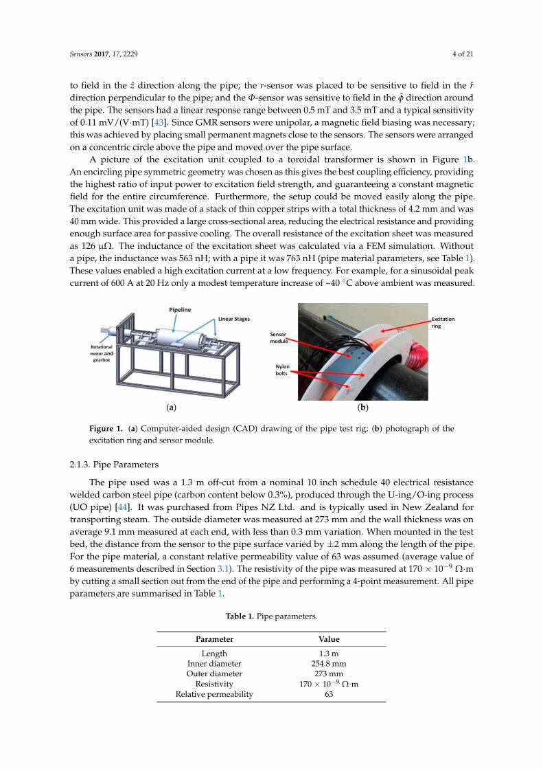
the system is shown in Figure 1a. The test rig included a support structure, linear motors for moving

the excitation unit and sensor module along the pipe, and a rotational motor and gearbox to rotate the

pipe. Due to distortions of the magnetic field at the end of the pipe, typically data was collected only

within the central 700 mm. Typically, a full pipe scan of 360 around the pipe with 5 resolution and

along the pipe with 5 mm resolution was undertaken; every measurement was carried out 5 times and

the average values plotted as a contour map of the pipe surface.

2.1.2. Magnetic Field Sensor and Excitation System

The measurement system consisted of a sensor module which is mounted directly above the

excitation sheet containing the GMR sensors and off-the-shelf instrumentation for processing the data

and communicating with the main LabVIEW program, run from a laptop computer.

The sensor module consisted of 3 perpendicularly aligned off-the-shelf GMR sensors from GMR

sensor manufacturer NVE cooperation (Model AA004) [43]. The z-sensor was placed to be sensitive

Sensors 2017, 17, 2229 4 of 21

to field in the z direction along the pipe; the r-sensor was placed to be sensitive to field in the r

direction perpendicular to the pipe; and the Φ-sensor was sensitive to field in the φ direction around

the pipe. The sensors had a linear response range between 0.5 mT and 3.5 mT and a typical sensitivity

of 0.11 mV/(V·mT) [43]. Since GMR sensors were unipolar, a magnetic field biasing was necessary;

this was achieved by placing small permanent magnets close to the sensors. The sensors were arranged

on a concentric circle above the pipe and moved over the pipe surface.

A picture of the excitation unit coupled to a toroidal transformer is shown in Figure 1b.

An encircling pipe symmetric geometry was chosen as this gives the best coupling efficiency, providing

the highest ratio of input power to excitation field strength, and guaranteeing a constant magnetic

field for the entire circumference. Furthermore, the setup could be moved easily along the pipe.

The excitation unit was made of a stack of thin copper strips with a total thickness of 4.2 mm and was

40 mm wide. This provided a large cross-sectional area, reducing the electrical resistance and providing

enough surface area for passive cooling. The overall resistance of the excitation sheet was measured

as 126 µΩ. The inductance of the excitation sheet was calculated via a FEM simulation. Without

a pipe, the inductance was 563 nH; with a pipe it was 763 nH (pipe material parameters, see Table 1).

These values enabled a high excitation current at a low frequency. For example, for a sinusoidal peak

current of 600 A at 20 Hz only a modest temperature increase of ~40 C above ambient was measured.

Ω

(a) (b)

Figure 1. (a) Computer-aided design (CAD) drawing of the pipe test rig; (b) photograph of the

− Ω

− Ω

Figure 1. (a) Computer-aided design (CAD) drawing of the pipe test rig; (b) photograph of the

excitation ring and sensor module.

2.1.3. Pipe Parameters

The pipe used was a 1.3 m off-cut from a nominal 10 inch schedule 40 electrical resistance

welded carbon steel pipe (carbon content below 0.3%), produced through the U-ing/O-ing process

(UO pipe) [44]. It was purchased from Pipes NZ Ltd. and is typically used in New Zealand for

transporting steam. The outside diameter was measured at 273 mm and the wall thickness was on

average 9.1 mm measured at each end, with less than 0.3 mm variation. When mounted in the test

bed, the distance from the sensor to the pipe surface varied by ±2 mm along the length of the pipe.

For the pipe material, a constant relative permeability value of 63 was assumed (average value of

6 measurements described in Section 3.1). The resistivity of the pipe was measured at 170 × 10−9Ω·m

by cutting a small section out from the end of the pipe and performing a 4-point measurement. All pipe

parameters are summarised in Table 1.

Table 1. Pipe parameters.

Parameter Value

Length 1.3 mInner diameter 254.8 mmOuter diameter 273 mm

Resistivity 170 × 10−9Ω·m

Relative permeability 63

Sensors 2017, 17, 2229 5 of 21

2.2. FEM Simulations

Apart from the experimental investigation, 3-dimensional FEM simulations using the quasi-static

eddy current solver of Ansys Maxwell 3D were performed. This allowed the evaluation of a much

wider parameter space and more detailed investigation of magnetic field and eddy current distribution.

Since the change in magnetic field amplitude induced by a typical defect is 2–3 orders of magnitude

lower than the overall strength of the magnetic field, a mesh noise-reduction technique was used: firstly,

the fields were simulated with the defect set to the same material parameters as the pipe, especially

refining the mesh around the defect and magnetic sensor locations. Then, a second simulation using

the same mesh, but setting the defect material to vacuum, was performed. The resulting fields were

then subtracted from each other. This enabled a very precise calculation of the magnetic field amplitude

change due to a defect (see Section 3.2).

3. Results and Discussion

3.1. Defect-Free Pipe

The excitation used for the initial tests and simulations was set to 20 Hz, with a sinusoidal 300 A

peak current and lift-off of 33 mm between excitation sheet and pipe (this lift-off distance was designed

to accommodate the insulation and shield used later). Tests and simulations presented in 3.1 were

done without insulation or weather shield.

3.1.1. Analysis of the Magnetic Field Distribution and Induced Eddy Currents

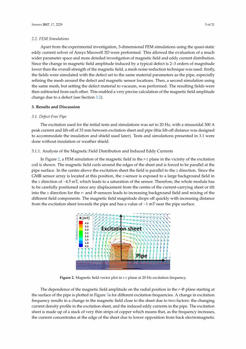
In Figure 2, a FEM simulation of the magnetic field in the r-z plane in the vicinity of the excitation

coil is shown. The magnetic field curls around the edges of the sheet and is forced to be parallel at the

pipe surface. In the centre above the excitation sheet the field is parallel to the z direction. Since the

GMR sensor array is located at this position, the z-sensor is exposed to a large background field in

the z direction of ~4.5 mT, which leads to a saturation of the sensor. Therefore, the whole module has

to be carefully positioned since any displacement from the centre of the current-carrying sheet or tilt

into the z direction for the r- and Φ-sensors leads to increasing background field and mixing of the

different field components. The magnetic field magnitude drops off quickly with increasing distance

from the excitation sheet towards the pipe and has a value of ~1 mT near the pipe surface.

Φ

Φ

Figure 2. Magnetic field vector plot in r-z plane at 20 Hz excitation frequency.

The dependence of the magnetic field amplitude on the radial position in the r-Φ plane starting at

the surface of the pipe is plotted in Figure 3a for different excitation frequencies. A change in excitation

frequency results in a change in the magnetic field close to the sheet due to two factors: the changing

current density profile in the excitation sheet, and the induced eddy currents in the pipe. The excitation

sheet is made up of a stack of very thin strips of copper which means that, as the frequency increases,

the current concentrates at the edge of the sheet due to lower opposition from back electromagnetic

Sensors 2017, 17, 2229 6 of 21

fields (EMFs) [45]. The current drops in the centre of the sheet and increases at the edge with increasing

frequency. This results in a decrease in the magnetic field in the centre and an increase at the edge.

A much stronger effect, however, is caused by the pipe, since induced eddy currents oppose and lower

the field between the pipe and excitation sheet. Also the field lines are diverted and concentrated due

to the presence of the pipe so the field amplitude decreases nearly linearly from the sheet edge to the

pipe surface. Outside the pipe and sheet, the field decays as 1/r (see Figure 3a).

Once we know the applied field at the surface of the pipe from our FEM simulation, the induced

eddy currents inside the pipe can be calculated analytically from the applied field,→

H = H0zeiωt z.

The currents could also be calculated by FEM, but the analytical results make it easier to produce data

for a wide range of geometries. By combining Faraday’s equation, Ampere’s law and the sinusoidal

time dependence, it can be shown that the electric field follows Bessel’s equation,

d2Eφ

dυ2+

1

υ

dEφ

dυ+

(

1 −1

υ2

)

Eφ = 0, (1)

with υ = k0r(i + 1) and k0 =√

ωµσ/2. The general solution for the electric field is

Eφ = Am J1(ν) + BmY1(ν) (2)

where J1 and Y1 are the Bessel and Neumann functions of first order. Likewise, the solution for the

magnetic field inside the pipe is

Hz =k0(i + 1)

iµω(Am J0(ν) + BmY0(ν)) (3)

where J0 and Y0 are the Bessel and Neumann functions of zero order. The constants Am and Bm can be

determined by applying the boundary condition that Hz must be continuous at the metal-air interfaces

and using the values for the applied field amplitudes H0z calculated by the FEM. We can then use

Jφ = σEφ (4)

to calculate the eddy currents.

The result for a subset of frequencies is shown in Figure 3b. This shows the expected behaviour:

at higher frequencies the current magnitude decays more rapidly from the outer surface, i.e., in common

terminology the skin depth is smaller. The surface current density is higher at higher frequencies in

line with the higher H0 at the surface, as seen in Figure 3a.

茎屎屎王 = 茎待佃結沈摘痛権鳥鉄帳這鳥鄭鉄 + 怠鄭 鳥帳這鳥鄭 + 岾な − 怠鄭鉄峇 継笛 = ど鉱 = 倦待堅岫件 + な岻 倦待 = 紐降航購 に⁄ 継笛 = 畦陳蛍怠岫荒岻 + 稽陳桁怠岫荒岻

茎佃 = 倦待岫件 + な岻件航降 岫畦陳蛍待岫荒岻 + 稽陳桁待岫荒岻岻

蛍笛 = 購継笛

(a) (b)

Figure 3. (a) Magnetic field magnitude in the r-Φ plane, through the centre of the excitation sheetFigure 3. (a) Magnetic field magnitude in the r-Φ plane, through the centre of the excitation sheet versus

distance from the pipe surface in the r direction at selected frequencies (5–200 Hz), calculated by the finite

element method (FEM); (b) eddy current density in the pipe wall from inner radius to outer radius at

selected frequencies (5–200 Hz), calculated analytically using the field values calculated by FEM.

Sensors 2017, 17, 2229 7 of 21

3.1.2. Measurements of Magnetic Field Distribution of a Bare Pipe

In Figure 4a the measurement of the magnetic field amplitude of the r-sensor over the pipe surface

is shown, with excitation of 20 Hz and 300 A. The average value over the whole pipe surface was

around 320 µT. A similar value was found for the Φ-sensor. The non-zero value could be attributed

to a non-perfect alignment of the sensors; the value found corresponded to a small tilt (~4) of the

sensors into the main field in the z direction.

When the end of the pipe was reached a rapid increase in the field amplitude was observed.

This was due to two different effects: firstly, as the excitation ring nears the end of the pipe,

the impedance of the excitation ring drops because the amount of steel that is acting as a core decreases.

This results in an increase in current and thus field, as the drive is a constant voltage. Secondly,

by reaching the end of the pipe the magnetic field lines start to curl in the r direction increasing the

field value in the r-sensor. This is also consistent with the finding that the r-sensor is more strongly

affected at the end of the pipe than the Φ-sensor.

In order to account for this influence, a correction algorithm was developed: To account for

the increasing current, the current was measured at each measurement location. This was done by

stepping the driving voltage from 0.1 V to 10 V in steps of 0.1 V, fitting the current field amplitude

with a linear function. This relationship was then used to correct the measured field amplitude to the

nominal 300 A level for each measurement.

To account for the effect of deviation of the field at the end of the pipe, a second algorithm was

applied. This algorithm first calculates the median value for each line of points around the pipe at each

z position. The difference between this z position median and the median value for the whole pipe is

calculated and added to all the data at this z position. This algorithm proved to be more effective than

the current correction algorithm, suggesting that the dominant cause of the increase in field along the z

axis is the effect of the fringe field rather than the drifting excitation current.

Once these factors are removed, the next major inhomogeneity of the magnetic field is revealed

(Figure 4b): stripes of similar magnetic field amplitude along the z axis. The most likely source of this

variation is a permeability variation around the pipe.

Overall, we expect the variations in pipe permeability to be a major influence. There is no

comprehensive understanding or database available that describes how the manufacturing process

and pipe usage e.g., thermal cycling, influence the permeability distribution. The literature mainly

reports on permeability variations produced by a seamless production process, which induces a helical

permeability variation seen in magnetic flux testing as “seamless pipe noise” [46]. Although the

literature reports on failures and stress distribution of UO-produced pipes [44], we did not find reports

regarding their magnetic properties.

In an attempt to quantify the variations due to permeability changes, permeability measurements

were performed on 6 samples of material removed from the pipe at different Φ values. The value

of the relative permeability varied between 20 and 128, with an average value of 63. Plotting the

permeability value versus the magnetic field amplitude for the 6 different locations gave inconclusive

data, possibly because drilling samples from the pipe can affect the permeability due to stress changes

in the material. First, simple FEM simulations of pipes with permeability variations indicate that large

area permeability variations can cause magnetic field patterns, as seen here. Furthermore, permeability

gradients can produce magnetic field variations similar to defect signals, as described in 3.3.1. The same

simulations as well as literature [37] indicate that, by using a multi-frequency algorithm, the response

for a defect can probably be separated from the response of a permeability variation.

Nevertheless, since for this pipe the observed magnetic field variation shows a simple stripe

pattern, in order to achieve a more homogeneous background a third simple algorithm was applied.

Essentially, this algorithm removes the stripe pattern by normalizing the median magnetic field value

for each angular position to the median overall value. This is done by calculating the median value

for all points along one angular position of the pipe and then subtracting this value from the median

value of the whole pipe. This correction value is then added to each data point at the angular position.

Sensors 2017, 17, 2229 8 of 21

(a) (b) (c)

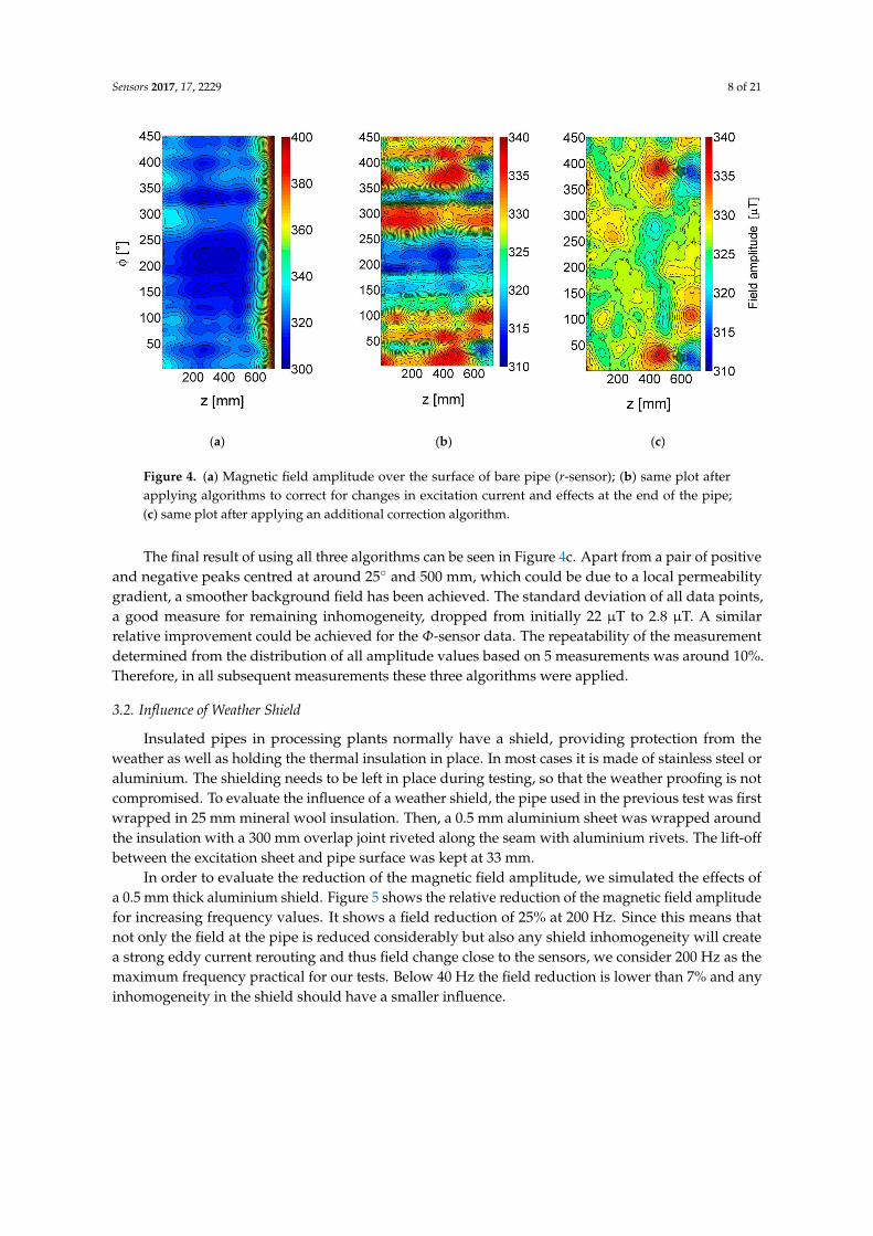
Figure 4. (a) Magnetic field amplitude over the surface of bare pipe (r-sensor); (b) same plot after

Φ

Figure 4. (a) Magnetic field amplitude over the surface of bare pipe (r-sensor); (b) same plot after

applying algorithms to correct for changes in excitation current and effects at the end of the pipe;

(c) same plot after applying an additional correction algorithm.

The final result of using all three algorithms can be seen in Figure 4c. Apart from a pair of positive

and negative peaks centred at around 25 and 500 mm, which could be due to a local permeability

gradient, a smoother background field has been achieved. The standard deviation of all data points,

a good measure for remaining inhomogeneity, dropped from initially 22 µT to 2.8 µT. A similar

relative improvement could be achieved for the Φ-sensor data. The repeatability of the measurement

determined from the distribution of all amplitude values based on 5 measurements was around 10%.

Therefore, in all subsequent measurements these three algorithms were applied.

3.2. Influence of Weather Shield

Insulated pipes in processing plants normally have a shield, providing protection from the

weather as well as holding the thermal insulation in place. In most cases it is made of stainless steel or

aluminium. The shielding needs to be left in place during testing, so that the weather proofing is not

compromised. To evaluate the influence of a weather shield, the pipe used in the previous test was first

wrapped in 25 mm mineral wool insulation. Then, a 0.5 mm aluminium sheet was wrapped around

the insulation with a 300 mm overlap joint riveted along the seam with aluminium rivets. The lift-off

between the excitation sheet and pipe surface was kept at 33 mm.

In order to evaluate the reduction of the magnetic field amplitude, we simulated the effects of

a 0.5 mm thick aluminium shield. Figure 5 shows the relative reduction of the magnetic field amplitude

for increasing frequency values. It shows a field reduction of 25% at 200 Hz. Since this means that

not only the field at the pipe is reduced considerably but also any shield inhomogeneity will create

a strong eddy current rerouting and thus field change close to the sensors, we consider 200 Hz as the

maximum frequency practical for our tests. Below 40 Hz the field reduction is lower than 7% and any

inhomogeneity in the shield should have a smaller influence.

Sensors 2017, 17, 2229 9 of 21

duction of the magnetic field amplitude due to a 0.5 mm aluFigure 5. Relative reduction of the magnetic field amplitude due to a 0.5 mm aluminium shield for

different excitation frequency values (FEM simulation).

In order to measure and quantify the influence of the aluminium shield, a set of tests was

undertaken from 5 Hz to 200 Hz. Normalized contour plots of the r field amplitude data at 20 Hz with,

and without the weather shield, are shown in Figure 6. Without the weather shield, a more or less

smooth background was found with only a small variation around the median value as expected from

the measurements discussed earlier. With the weather shield, a distinct negative and positive peak pair

centred at around 50 and 200 mm with a change in field amplitude of around 200 µT peak-to-peak

appeared. The signal was likely generated from the outside edge of the aluminium shield where the

shield is riveted to the inside. At this point the eddy currents induced in the shield are required to

make a rapid change in direction which, in turn, causes a change in the magnetic field.

Without weather shield With weather shield

Figure 6. Change in magnetic field amplitude (r-sensor) without (left) and with (right) 0.5 mm thick Figure 6. Change in magnetic field amplitude (r-sensor) without (left) and with (right) 0.5 mm thick

aluminium weather shield; 20 Hz, 300 A excitation frequency.

In processing plants, defects and dents (e.g., due to a heavy physical impact) are often present

in the shield. To investigate their influence in a second experiment, artificial dents were introduced

and the same measurements performed. In Figure 7 contour plots of the r-sensor field amplitude

change at 5 Hz, 20 Hz and 200 Hz are shown. The 5 Hz data show a noisy background and a weak

indication of the shield overlap around 50, but no clear signal from the dented aluminium, since most

Sensors 2017, 17, 2229 10 of 21

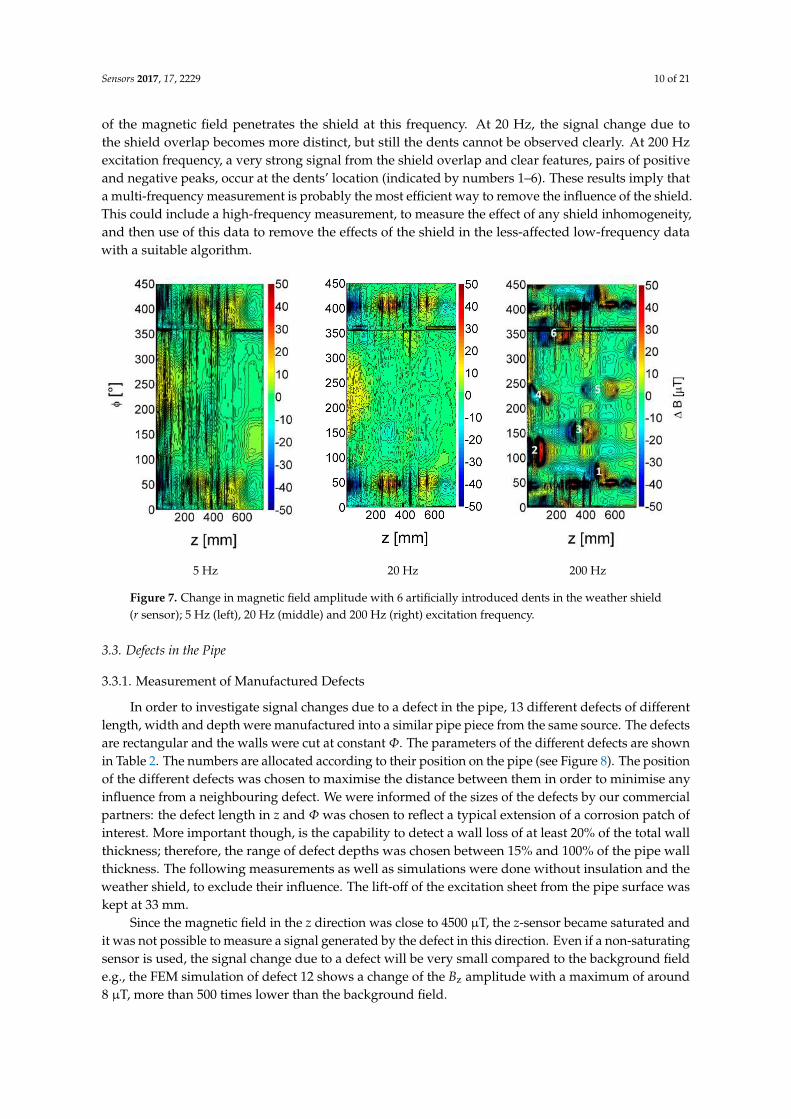
of the magnetic field penetrates the shield at this frequency. At 20 Hz, the signal change due to

the shield overlap becomes more distinct, but still the dents cannot be observed clearly. At 200 Hz

excitation frequency, a very strong signal from the shield overlap and clear features, pairs of positive

and negative peaks, occur at the dents’ location (indicated by numbers 1–6). These results imply that

a multi-frequency measurement is probably the most efficient way to remove the influence of the shield.

This could include a high-frequency measurement, to measure the effect of any shield inhomogeneity,

and then use of this data to remove the effects of the shield in the less-affected low-frequency data

with a suitable algorithm.

5 Hz 20 Hz 200 Hz

Figure 7. Change in magnetic field amplitude with 6 artificially introduced dents in the weather

Φ

Φ

Φ

Figure 7. Change in magnetic field amplitude with 6 artificially introduced dents in the weather shield

(r sensor); 5 Hz (left), 20 Hz (middle) and 200 Hz (right) excitation frequency.

3.3. Defects in the Pipe

3.3.1. Measurement of Manufactured Defects

In order to investigate signal changes due to a defect in the pipe, 13 different defects of different

length, width and depth were manufactured into a similar pipe piece from the same source. The defects

are rectangular and the walls were cut at constant Φ. The parameters of the different defects are shown

in Table 2. The numbers are allocated according to their position on the pipe (see Figure 8). The position

of the different defects was chosen to maximise the distance between them in order to minimise any

influence from a neighbouring defect. We were informed of the sizes of the defects by our commercial

partners: the defect length in z and Φ was chosen to reflect a typical extension of a corrosion patch of

interest. More important though, is the capability to detect a wall loss of at least 20% of the total wall

thickness; therefore, the range of defect depths was chosen between 15% and 100% of the pipe wall

thickness. The following measurements as well as simulations were done without insulation and the

weather shield, to exclude their influence. The lift-off of the excitation sheet from the pipe surface was

kept at 33 mm.

Since the magnetic field in the z direction was close to 4500 µT, the z-sensor became saturated and

it was not possible to measure a signal generated by the defect in this direction. Even if a non-saturating

sensor is used, the signal change due to a defect will be very small compared to the background field

e.g., the FEM simulation of defect 12 shows a change of the Bz amplitude with a maximum of around

8 µT, more than 500 times lower than the background field.

Sensors 2017, 17, 2229 11 of 21

Contrary to this behaviour, Φ- and r-sensors only experience a background field due to the tilt

into the main field; this means the expected background field is much lower and easier to account for,

as discussed in Section 3.1.

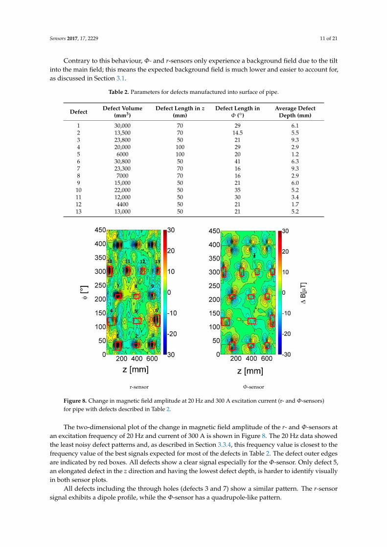
Table 2. Parameters for defects manufactured into surface of pipe.

DefectDefect Volume

(mm3)Defect Length in z

(mm)Defect Length in

Φ ()Average Defect

Depth (mm)

1 30,000 70 29 6.12 13,500 70 14.5 5.53 23,800 50 21 9.34 20,000 100 29 2.95 6000 100 20 1.26 30,800 50 41 6.37 23,300 70 16 9.38 7000 70 16 2.99 15,000 50 21 6.010 22,000 50 35 5.211 12,000 50 30 3.412 4400 50 21 1.713 13,000 50 21 5.2

Φ

r-sensor Φ-sensor

Figure 8. Change in magnetic field amplitude at 20 Hz and 300 A excitation current (r- and

Φ

Φ

Φ

Φ

Φ

Figure 8. Change in magnetic field amplitude at 20 Hz and 300 A excitation current (r- and Φ-sensors)

for pipe with defects described in Table 2.

The two-dimensional plot of the change in magnetic field amplitude of the r- and Φ-sensors at

an excitation frequency of 20 Hz and current of 300 A is shown in Figure 8. The 20 Hz data showed

the least noisy defect patterns and, as described in Section 3.3.4, this frequency value is closest to the

frequency value of the best signals expected for most of the defects in Table 2. The defect outer edges

are indicated by red boxes. All defects show a clear signal especially for the Φ-sensor. Only defect 5,

an elongated defect in the z direction and having the lowest defect depth, is harder to identify visually

in both sensor plots.

All defects including the through holes (defects 3 and 7) show a similar pattern. The r-sensor

signal exhibits a dipole profile, while the Φ-sensor has a quadrupole-like pattern.

Sensors 2017, 17, 2229 12 of 21

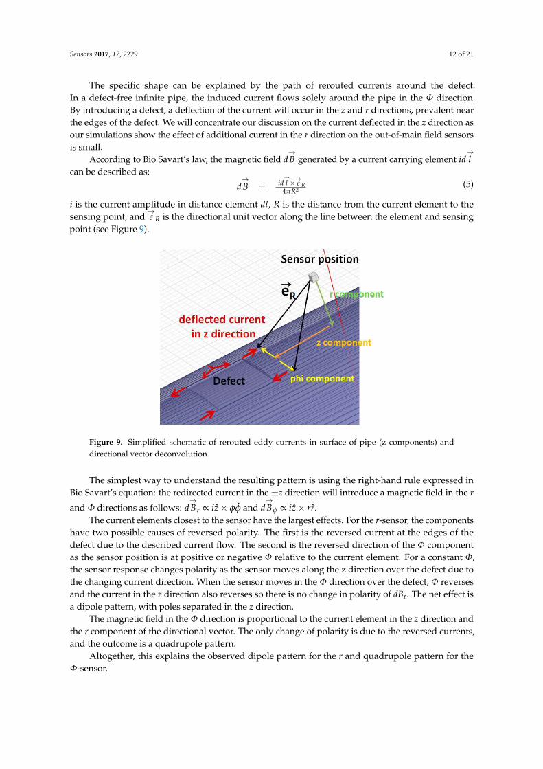
The specific shape can be explained by the path of rerouted currents around the defect.

In a defect-free infinite pipe, the induced current flows solely around the pipe in the Φ direction.

By introducing a defect, a deflection of the current will occur in the z and r directions, prevalent near

the edges of the defect. We will concentrate our discussion on the current deflected in the z direction as

our simulations show the effect of additional current in the r direction on the out-of-main field sensors

is small.

According to Bio Savart’s law, the magnetic field d→

B generated by a current carrying element id→

l

can be described as:

d→

B = id→

l ×→e R

4πR2(5)

i is the current amplitude in distance element dl, R is the distance from the current element to the

sensing point, and→

e R is the directional unit vector along the line between the element and sensing

point (see Figure 9).

穴稽屎王件穴健王穴稽屎王 = 件穴 健王× 結王眺4講迎態穴健蚕屎王三

Φ 穴稽屎王追 ∝ 件権 × 剛剛侮 穴稽屎王笛 ∝ 件権 × 堅堅Φ

ΦΦ

ΦΦ

Φ

Φ

Δ Φ

Figure 9. Simplified schematic of rerouted eddy currents in surface of pipe (z components) and

directional vector deconvolution.

The simplest way to understand the resulting pattern is using the right-hand rule expressed in

Bio Savart’s equation: the redirected current in the ±z direction will introduce a magnetic field in the r

and Φ directions as follows: d→

B r ∝ iz × φφ and d→

Bφ ∝ iz × rr.

The current elements closest to the sensor have the largest effects. For the r-sensor, the components

have two possible causes of reversed polarity. The first is the reversed current at the edges of the

defect due to the described current flow. The second is the reversed direction of the Φ component

as the sensor position is at positive or negative Φ relative to the current element. For a constant Φ,

the sensor response changes polarity as the sensor moves along the z direction over the defect due to

the changing current direction. When the sensor moves in the Φ direction over the defect, Φ reverses

and the current in the z direction also reverses so there is no change in polarity of dBr. The net effect is

a dipole pattern, with poles separated in the z direction.

The magnetic field in the Φ direction is proportional to the current element in the z direction and

the r component of the directional vector. The only change of polarity is due to the reversed currents,

and the outcome is a quadrupole pattern.

Altogether, this explains the observed dipole pattern for the r and quadrupole pattern for the

Φ-sensor.

Sensors 2017, 17, 2229 13 of 21

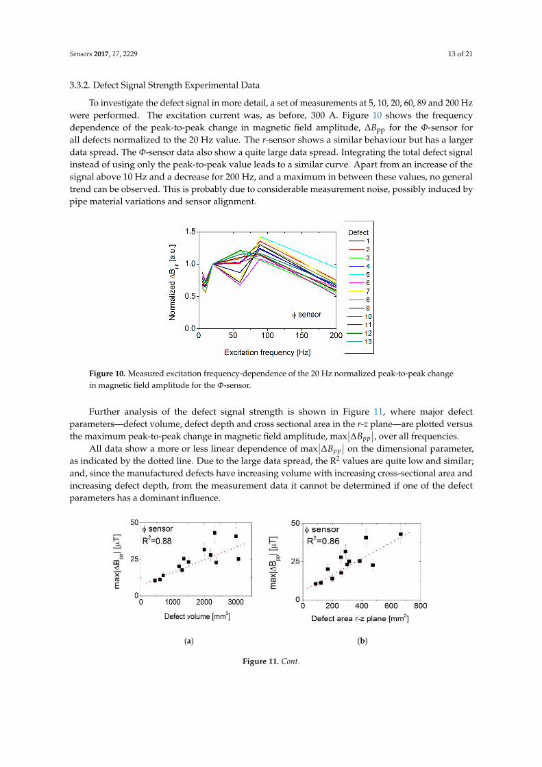
3.3.2. Defect Signal Strength Experimental Data

To investigate the defect signal in more detail, a set of measurements at 5, 10, 20, 60, 89 and 200 Hz

were performed. The excitation current was, as before, 300 A. Figure 10 shows the frequency

dependence of the peak-to-peak change in magnetic field amplitude, ∆Bpp for the Φ-sensor for

all defects normalized to the 20 Hz value. The r-sensor shows a similar behaviour but has a larger

data spread. The Φ-sensor data also show a quite large data spread. Integrating the total defect signal

instead of using only the peak-to-peak value leads to a similar curve. Apart from an increase of the

signal above 10 Hz and a decrease for 200 Hz, and a maximum in between these values, no general

trend can be observed. This is probably due to considerable measurement noise, possibly induced by

pipe material variations and sensor alignment.

Φ

Φ

弁∆稽椎椎弁弁∆稽椎椎弁

Figure 10. Measured excitation frequency-dependence of the 20 Hz normalized peak-to-peak change

in magnetic field amplitude for the Φ-sensor.

Further analysis of the defect signal strength is shown in Figure 11, where major defect

parameters—defect volume, defect depth and cross sectional area in the r-z plane—are plotted versus

the maximum peak-to-peak change in magnetic field amplitude, max∣

∣∆Bpp

∣

∣, over all frequencies.

All data show a more or less linear dependence of max∣

∣∆Bpp

∣

∣ on the dimensional parameter,

as indicated by the dotted line. Due to the large data spread, the R2 values are quite low and similar;

and, since the manufactured defects have increasing volume with increasing cross-sectional area and

increasing defect depth, from the measurement data it cannot be determined if one of the defect

parameters has a dominant influence.

Φ

Φ

弁∆稽椎椎弁弁∆稽椎椎弁

(a) (b)

Figure 11. Cont.

Sensors 2017, 17, 2229 14 of 21

(c)

e of maximum peak-to-peak change in magneti

弁∆稽椎椎弁Φ

Φ

Φ

Φ

Φ

Figure 11. Dependence of maximum peak-to-peak change in magnetic field amplitude on (a) defect

volume, (b) defect area in the r–z plane, and (c) defect depth.

3.3.3. Validation of FEM Simulations

To investigate the dependence of the defect signal in more detail, FEM simulations were performed.

Since the excitation current of 300 A was quite large, and the FEM solver assumes a linear constitutional

behaviour between magnetic field and excitation current, an experimental test was performed first.

In Figure 12a, the measured relationship between max∣

∣∆Bpp

∣

∣ normalized to the 300 A value for the

Φ-sensor is shown for all defects for an excitation current between 100 A and 500 A. This shows a linear

relationship with a relative increase of ~20% every 100 A. This means that the assumption of linear

constitutional behaviour of magnetic field amplitude and excitation current in the FEM solver is valid.

In order to validate the FEM simulations, a direct comparison of the simulated and measured

defect signals was made. In Figure 12b, the Φ-sensor signal at 20 Hz excitation frequency and 300 A

excitation current along the z axis is shown for 3 different defects: the defect with the lowest volume

(Nr 12), the corresponding through hole (Nr 3), and a large defect with average depth extended in the

z as well as the Φ directions (Nr 4). It can be seen that there is reasonable agreement between FEM

simulations and experimental data. The average deviation between measured and simulated data is

between 20% and 40%, and other simulated defects and the r-sensor data show a similar agreement.

The deviations are likely due to local variations of permeability around the defect; the FEM simulations

assumed a constant permeability of 63. Nevertheless, these data show that the FEM simulation can be

used to determine the influence of defect parameters.

弁∆稽椎椎弁Φ

Φ

Φ

(a) (b)

Figure 12. (a) Maximum peak-to-peak change in magnetic field amplitude for the Φ-sensor

Φ

Figure 12. (a) Maximum peak-to-peak change in magnetic field amplitude for the Φ-sensor normalized

to 300 A; (b) comparison of measured and FEM simulation results of change in magnetic field amplitude

for the Φ-sensor located at the defect edge and moving over the defect in the z direction.

Sensors 2017, 17, 2229 15 of 21

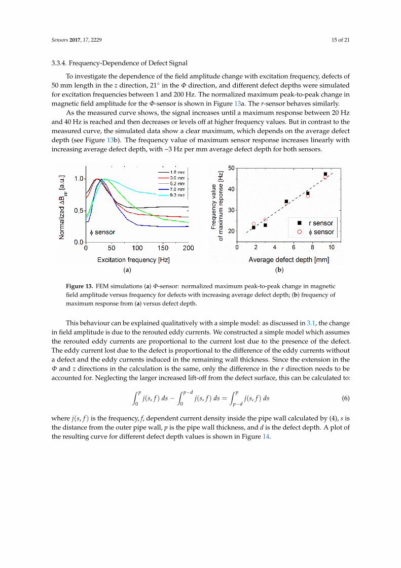
3.3.4. Frequency-Dependence of Defect Signal

To investigate the dependence of the field amplitude change with excitation frequency, defects of

50 mm length in the z direction, 21 in the Φ direction, and different defect depths were simulated

for excitation frequencies between 1 and 200 Hz. The normalized maximum peak-to-peak change in

magnetic field amplitude for the Φ-sensor is shown in Figure 13a. The r-sensor behaves similarly.

As the measured curve shows, the signal increases until a maximum response between 20 Hz

and 40 Hz is reached and then decreases or levels off at higher frequency values. But in contrast to the

measured curve, the simulated data show a clear maximum, which depends on the average defect

depth (see Figure 13b). The frequency value of maximum sensor response increases linearly with

increasing average defect depth, with ~3 Hz per mm average defect depth for both sensors.

Φ

Φ

(a) (b)

Figure 13. FEM simulations (a) Φ-sensor: normalized maximum peak-to-peak change in magnetic

Φ

完 倹岫嫌, 血岻穴嫌椎待 完 倹岫嫌, 血岻 穴嫌椎貸鳥待 = 完 倹岫嫌, 血岻 穴嫌椎椎貸鳥倹岫嫌, 血岻

Figure 13. FEM simulations (a) Φ-sensor: normalized maximum peak-to-peak change in magnetic

field amplitude versus frequency for defects with increasing average defect depth; (b) frequency of

maximum response from (a) versus defect depth.

This behaviour can be explained qualitatively with a simple model: as discussed in 3.1, the change

in field amplitude is due to the rerouted eddy currents. We constructed a simple model which assumes

the rerouted eddy currents are proportional to the current lost due to the presence of the defect.

The eddy current lost due to the defect is proportional to the difference of the eddy currents without

a defect and the eddy currents induced in the remaining wall thickness. Since the extension in the

Φ and z directions in the calculation is the same, only the difference in the r direction needs to be

accounted for. Neglecting the larger increased lift-off from the defect surface, this can be calculated to:

∫ p

0j(s, f ) ds −

∫ p−d

0j(s, f ) ds =

∫ p

p−dj(s, f ) ds (6)

where j(s, f ) is the frequency, f, dependent current density inside the pipe wall calculated by (4), s is

the distance from the outer pipe wall, p is the pipe wall thickness, and d is the defect depth. A plot of

the resulting curve for different defect depth values is shown in Figure 14.

Sensors 2017, 17, 2229 16 of 21

Φ

Φ

Φ −

Φ −

− Φ −

Φ

Φ

Φ

Figure 14. Normalized peak-to-peak change in magnetic field amplitude versus frequency for defects

with increasing defect depth using Formula (6).

The calculated curve shows a qualitatively similar dependence as the FEM simulation in

Figure 13a: increasing field amplitude until a maximum is reached, and levelling off at higher frequency

values. Also, the maximum of the response shifts with increasing defect depth. The absolute value

of the frequency where the maximum occurs as well as the increase per mm defect depth is higher

than the FEM simulated response, especially for deep defects; the curve is also wider. There are

probably several reasons for the deviation: the surface current at the bottom of the defect is not only

dependent on the increased distance from the excitation sheet but also the surrounding remaining

material. Notably, the proportion of the induced current that is redirected around the defect probably

depends on the exact shape and remaining wall thickness in a more complex way, which means this

simple model can only explain qualitative behaviour.

3.3.5. Influence of Defect Dimension on Signal Strength

Since from the experimental data the influence of the defect dimensions in the r, Φ and z directions

could not be determined, another set of FEM simulations was performed.

In order to distinguish the influence between defect volume and defect depth, a FEM simulation

was undertaken of 5 rectangular defects with a constant average depth of 5.2 mm but different

defect size in the Φ and z directions and thus different volumes, in a similar range as the measured

defects. The frequency of the maximum signal occurred at the same frequency value at around 30 Hz,

as expected from simulations discussed before. A linear dependence between the defect volume and

Φ and r peak-to-peak field amplitude change was found, with 1.2 × 10−3µT/mm3 for the Φ-sensor

and 1.4 × 10−3µT/mm3 for the r-sensor (see Figure 15a). This agrees well with the experimental

data: 1.3 × 10−3µT/mm3 for the Φ-sensor and 1.6 × 10−3

µT/mm3 for the r-sensor. The simulated

defect volumes change by 1320%, the defect signal change spans a similar range: r signal 570% and Φ

signal 2000%.

A second simulation was undertaken, keeping the volume in a narrow range of 11,000–15,000 mm3

but varying the defect depth between 1.8 mm and 8.7 mm. The volume normalized magnetic field

amplitude change of the Φ-sensor at the defect edge was very similar for all depths, apart from the

very large and shallow defect, as shown in Figure 15b. This means that the defect depth alone only has

a small influence on the signal strength.

In order to distinguish between the influence of the defect volume and the defect cross-sectional

area, a third simulation was undertaken. The volume was kept constant to 13,200 mm3 and the average

defect depth constant to 5.2 mm. The cross-sectional area was changed within the same range as the

measured defects between 100 mm2 and 700 mm2. In Figure 15c, the cross-sectional area in the r–z

plane is plotted versus the maximum peak-to-peak magnetic field amplitude change. A more complex

non-linear influence exists, but the defect signal variation is only 60% for the r-sensor and 115% for the

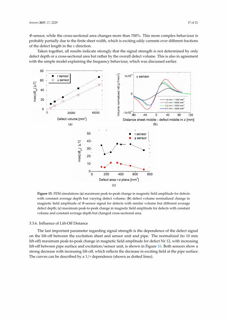
Sensors 2017, 17, 2229 17 of 21

Φ-sensor, while the cross-sectional area changes more than 700%. This more complex behaviour is

probably partially due to the finite sheet width, which is exciting eddy currents over different fractions

of the defect length in the z direction.

Taken together, all results indicate strongly that the signal strength is not determined by only

defect depth or a cross-sectional area but rather by the overall defect volume. This is also in agreement

with the simple model explaining the frequency behaviour, which was discussed earlier.

(a) (b)

(c)

Figure 15. FEM simulations (a) maximum peak-to-peak change in magnetic field amplitude for

Φ

Figure 15. FEM simulations (a) maximum peak-to-peak change in magnetic field amplitude for defects

with constant average depth but varying defect volume; (b) defect volume normalized change in

magnetic field amplitude of Φ-sensor signal for defects with similar volume but different average

defect depth; (c) maximum peak-to-peak change in magnetic field amplitude for defects with constant

volume and constant average depth but changed cross-sectional area.

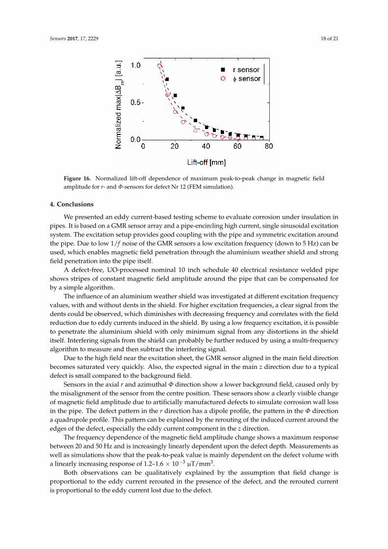
3.3.6. Influence of Lift-Off Distance

The last important parameter regarding signal strength is the dependence of the defect signal

on the lift-off between the excitation sheet and sensor unit and pipe. The normalized (to 10 mm

lift-off) maximum peak-to-peak change in magnetic field amplitude for defect Nr 12, with increasing

lift-off between pipe surface and excitation/sensor unit, is shown in Figure 16. Both sensors show a

strong decrease with increasing lift-off, which reflects the decrease in exciting field at the pipe surface.

The curves can be described by a 1/r dependence (shown as dotted lines).

Sensors 2017, 17, 2229 18 of 21

Φ

Φ

Φ

−

Figure 16. Normalized lift-off dependence of maximum peak-to-peak change in magnetic field

amplitude for r- and Φ-sensors for defect Nr 12 (FEM simulation).

4. Conclusions

We presented an eddy current-based testing scheme to evaluate corrosion under insulation in

pipes. It is based on a GMR sensor array and a pipe-encircling high current, single sinusoidal excitation

system. The excitation setup provides good coupling with the pipe and symmetric excitation around

the pipe. Due to low 1/f noise of the GMR sensors a low excitation frequency (down to 5 Hz) can be

used, which enables magnetic field penetration through the aluminium weather shield and strong

field penetration into the pipe itself.

A defect-free, UO-processed nominal 10 inch schedule 40 electrical resistance welded pipe

shows stripes of constant magnetic field amplitude around the pipe that can be compensated for

by a simple algorithm.

The influence of an aluminium weather shield was investigated at different excitation frequency

values, with and without dents in the shield. For higher excitation frequencies, a clear signal from the

dents could be observed, which diminishes with decreasing frequency and correlates with the field

reduction due to eddy currents induced in the shield. By using a low frequency excitation, it is possible

to penetrate the aluminium shield with only minimum signal from any distortions in the shield

itself. Interfering signals from the shield can probably be further reduced by using a multi-frequency

algorithm to measure and then subtract the interfering signal.

Due to the high field near the excitation sheet, the GMR sensor aligned in the main field direction

becomes saturated very quickly. Also, the expected signal in the main z direction due to a typical

defect is small compared to the background field.

Sensors in the axial r and azimuthal Φ direction show a lower background field, caused only by

the misalignment of the sensor from the centre position. These sensors show a clearly visible change

of magnetic field amplitude due to artificially manufactured defects to simulate corrosion wall loss

in the pipe. The defect pattern in the r direction has a dipole profile, the pattern in the Φ direction

a quadrupole profile. This pattern can be explained by the rerouting of the induced current around the

edges of the defect, especially the eddy current component in the z direction.

The frequency dependence of the magnetic field amplitude change shows a maximum response

between 20 and 50 Hz and is increasingly linearly dependent upon the defect depth. Measurements as

well as simulations show that the peak-to-peak value is mainly dependent on the defect volume with

a linearly increasing response of 1.2–1.6 × 10−3µT/mm3.

Both observations can be qualitatively explained by the assumption that field change is

proportional to the eddy current rerouted in the presence of the defect, and the rerouted current

is proportional to the eddy current lost due to the defect.

Sensors 2017, 17, 2229 19 of 21

Increasing insulation thickness means increasing lift-off between the pipe surface and excitation

sheet leads to a decreased defect signal and can be described with a 1/r dependence.

Taken together, the results suggest that our approach is well suited for measuring and quantifying

corrosion under insulation. Based upon our concept, a field-ready prototype tool including

a multi-frequency measurement, targeting insulation thickness of up to two inches, is being built

and tested.

Acknowledgments: The contents of this article are the subject of one or more patents and/or patent applications.This work was supported by the New Zealand Ministry of Business, Innovation and Employment under theprogram C08X1206 “Magnetic devices for security, non-destructive testing and instrumentation”. Financialsupport from Quest Integrated, LLC. is gratefully acknowledged. We would like to thank P. Bondurant andT. Mactutis (Quest Integrated LLC.), as well as K. Stevens and D. Drabble (Quest Integrity NZ Ltd.) for fruitfuldiscussions and support. We would also like to thank S. Granville, Robinson Research Institute, for the pipepermeability and conductivity measurements.

Author Contributions: J.B. built the pipe test setup, designed, performed and evaluated the experiments,analyzed the experimental data, provided input for the theoretical models and wrote parts of the manuscript.N.L. performed the theoretical calculations and wrote parts of the manuscript. A.H. performed the FEMsimulations, provided input for the theoretical models and wrote parts of the manuscript. The manuscriptwas revised and improved by all authors.

Conflicts of Interest: The authors declare no conflict of interest.

References

1. National Association of Corrosion Engineers, Corrosion Costs and Preventive Strategies in the United

States. 2014. Available online: http://www.nace.org/uploadedFiles/Publications/ccsupp.pdf (accessed on

18 August 2017).

2. Winnik, S. Corrosion-under-Insulation (CUI) Guidelines; Europaen Federation of Corrosion Publications No. 55;

Woodhead Publishing Limited: Cambridge, UK, 2016.

3. Winnik, S. Piping System CUI: Old Problem, Different Approaches, Minutes of EFC WP15 Corrosion in the Refinery

Industry; Budapest Congress Centre: Budapest, Hungary, 2003.

4. García-Martín, J.; Gómez-Gil, J.; Gar1Vázquez-Sánchez, E. Non-Destructive Techniques Based on Eddy

Current Testing. Sensors 2011, 11, 2525–2565. [CrossRef] [PubMed]

5. International Atomic Energy Agency. Development of Protocols for Corrosion and Deposits Evaluation in Pipes by

Radiography; IAEA-TECDOC-1445; International Atomic Energy Agency: Vienna, Austria, 2006.

6. Ong, P.; Patel, V.; Balasubramanyan, A. Quantitative characterization of corrosion under insulation.

J. Nondestruct. Eval. 1997, 16, 135–146. [CrossRef]

7. Abdullah, J.; Yahya, R. Application of CdZnTe Gamma-Ray Detector for Imaging Corrosion under Insulation.

AIP Conf. Proc. 2007, 909, 74–79.

8. Samir, A.; Balamesh, A. Imaging corrosion under insulation by gamma ray backscattering method.

In Proceedings of the 18th World Conference on Nondestructive Testing, Durban, South Africa,

16–20 April 2012.

9. Samir, A.; Balamesh, A. Single Side Imaging of Corrosion under Insulation Using Single Photon Gamma

Backscattering. Res. Nondestruct. Eval. 2014, 25, 172–185.

10. Zscherpel, U.; Ewert, U.; Infanzon, S.; Rastkhan, N.; Vaidya, P.; Einav, I.; Ekinci, S. Radiographic evaluation

of corrosion and deposits in pipes: Results of an IAEA co-ordinated research programme. In Proceedings of

the 9th European Conference on NDT DGZfP, Berlin, Germany, 25–29 September 2006.

11. Lopushansky, R.; Light, G.; Gupta, N. Digital radiography of process piping. In Proceedings of the SPIE

3398, Nondestructive Evaluation of Utilities and Pipes II, San Antonio, TX, USA, 31 March–4 April 1998.

12. Cawley, P.; Lowe, M.; Alleyne, D.; Pavlakovic, B.; Wilcox, P. Practical long range guided wave

inspection—Applications to pipes and rail. Mater. Eval. 2003, 61, 66–74.

13. Alleyne, D.; Pavlakovic, B.; Lowe, M.; Cawley, P. Rapid. Long Range Inspection of Chemical Plant Pipework

Using Guided Waves. Rev. Prog. QNDE 2001, 20, 180–187.

14. Rose, J.; Jiao, D.; Spanner, J. Ultrasonic Guided Waves for Piping Inspection. Rev. Prog. Quant. NDE 1996, 15,

1285–1290.

Sensors 2017, 17, 2229 20 of 21

15. Fateri, S.; Lowe, P.; Engineer, B.; Boulgouris, N. Investigation of Ultrasonic Guided Waves Interacting With

Piezoelectric Transducers. IEEE Sens. J. 2015, 15, 4319–4328. [CrossRef]

16. Demma, A.; Cawley, P.; Lowe, M.; Roosenbrand, A.; Pavlakovic, B. The reflection of guided waves from

notches in pipes: A guide for interpreting corrosion measurements. NDT E Int. 2003, 37, 167–180. [CrossRef]

17. Verma, B.; Mishra, T.; Balasubramaniam, K.; Rajagopal, P. Interaction of low-frequency axisymmetric

ultrasonic guided waves with bends in pipes of arbitrary bend angle and general bend radius. Ultrasonics

2014, 54, 801–808. [CrossRef] [PubMed]

18. Kwun, H.; Holt, A. Feasibility of under-lagging corrosion detection in steel pipe using the magnetostrictive

sensor technique. NDT E Int. 1995, 28, 211–214. [CrossRef]

19. TueV Sued. Detecting Corrosion under Insulation. E-ssentials 2012, 5, 2–4.

20. Jones, R.; Simonetti, F.; Lowe, M.; Bradley, I. Use of Microwaves for the Detection of Water as a Cause of

Corrosion under Insulation. J. Nondestruct. Eval. 2011, 31, 65–76. [CrossRef]

21. Jarvis, R.; Cawley, P.; Nagy, P. Current deflection NDE for the inspection and monitoring of pipes. NDT E Int.

2016, 81, 46–59. [CrossRef]

22. Garcıa-Martın, J.; Gomez-Gil, J.; Vazquez-Sanchez, E. Non-destructive techniques based on eddy current

testing. Sensors 2011, 11, 2525–2565. [CrossRef] [PubMed]

23. Uzal, E.; Rose, J. The impedance of eddy current probes above layered metals whose conductivity and

permeability vary continuously. IEEE Trans. Magn. 1993, 29, 1869–1873. [CrossRef]

24. Stutzke, N.; Russek, S.; Pappas, P. Low-frequency noise measurements on commercial magnetoresistive

magnetic field sensors. J. Appl. Phys. 2005, 97, 10Q107. [CrossRef]

25. Dogaru, T.; Smith, S.T. Giant magnetoresistence-based eddy-current sensor. IEEE Trans. Magn. 2002, 37,

3831–3838. [CrossRef]

26. Rifai, D.; Abdalla, A.; Ali, A.; Razali, R. Giant Magnetoresistance Sensors: A Review on Structures and

Non-Destructive Eddy Current Testing Applications. Sensors 2016, 16, 298. [CrossRef] [PubMed]

27. Nair, N.; Melapudi, V.; Hector, J.; Liu, X.; Deng, Y.; Zeng, Z.; Udpa, L.; Thomas, J.; Udpa, S. A GMR-based

eddy current system for NDE of aircraft structures. IEEE Trans. Magn. 2016, 42, 3312–3314. [CrossRef]

28. Yang, G.; Zeng, Z.; Deng, Y.; Liu, X.; Udpa, L.; Tamburrino, A. 3D EC-GMR sensor system for detection of

subsurface defects at steel fastener sites. NDT E Int. 2012, 50, 20–28. [CrossRef]

29. Lo, C.; Nakagawa, N. Evaluation of eddy current and magnetic techniques for inspecting rebars in bridge

barrier rails. AIP Conf. Proc. 2013, 1511, 1371–1377.

30. Yamada, S.; Chomsuwan, K.; Fukuda, Y.; Iwahara, M.; Wakiwaka, H.; Shoji, S. Eddy-current testing probe

with spin-valve type GMR sensor for printed circuit board inspection. IEEE Trans. Magn. 2004, 40, 2676–2678.

[CrossRef]

31. Wang, R.; Kawamura, Y. An automated sensing system for steel bridge inspection using GMR sensor array

and magnetic wheels of climbing robot. J. Sens. 2016. [CrossRef]

32. Du, W.; Nguyen, H.; Dutt, A.; Scallion, K. Design of a GMR sensor array system for robotic pipe inspection.

In Proceedings of the 2010 IEEE SENSORS, Kona, HI, USA, 1–4 November 2010; pp. 2551–2554.

33. Chen, L.; Que, P.; Jin, T. A giant-magnetoresistance sensor for magnetic-flux-leakage nondestructive testing

of a pipe. Russ. J. Nondestruct. Test. 2005, 41, 462–465. [CrossRef]

34. Kaack, M.; Orth, T.; Fischer, G.; Weingarten, W.; Koka, S.; Arzt, N. Application of GMR sensors for the

industrial inspection of seamless steel pipes. In Proceedings of the 11th Symposium on Magnetoresistive

Sensors and Magnetic Systems, Wetzlar, Germany, 29–30 March 2011.

35. Rifai, D.; Abdalla, A.; Razali, R.; Ali, K.; Faraj, M. An eddy current testing platform system for pipe defect

inspection based on an optimized eddy current technique probe design. Sensors 2017, 17. [CrossRef]

[PubMed]

36. Goldfine, N.; Dunford, T.; Washabaugh, A.; Haque, S.; Denenberg, S. MWM-Array Electromagnetic Techniques

for Crack Sizing, Weld Assessment, Wall Loss/Thickness Measurement and Mechanical Damage Profilometry;

Technical Document TR_2012_05_02(2012); Jentek sensors Inc.: Waltham, MA, USA, 2012.

37. Farea, S.; Hammad, R.; Dawoud, F.; Dossary, S.; Alzarani, S.; Binqorsain, A.; Minachi, A.; Goldfine, N.;

Denenberg, S.; Manning, B.; et al. Field Demonstrations of MR-MWM-Array Solution for Detection, Imaging

and Sizing of Corrosion under Fireproofing (CUF) with Wire Mesh. In Proceedings of the 15th Middle East

Corrosion Conference, Bahrain, 2–5 February 2014.

Sensors 2017, 17, 2229 21 of 21

38. Brett, C.; de Raad, J. Validation of pulsed eddy current system for measuring wall thinning trough insulation.

In Proceedings of the SPIE 2947, Nondestructive Evaluation of Utilities and Pipes, Scottsdale, AZ, USA,

14 November 1996.

39. Cheng, W. Pulsed Eddy Current Testing of Carbon Steel Pipes Wall-thinning Through Insulation and

Cladding. J. Nondestruct. Eval. 2012, 31, 215–224. [CrossRef]

40. Greiner, M.; Demers-Carpeneter, V.; Rochette, M.; Hardy, F. Pulsed Eddy Current: New Developments for

Corrosion under Insulation Examinations. In Proceedings of the 19th World Conference on Non-Destructive

Testing, Munich, Germany, 13–17 June 2016.

41. Majidnia, S.; Rudlin, J.; Nilavalan, R. A pulsed eddy current system for flaw detection using an encircling

coil on a steel pipe. In Proceedings of the First International Conference on Welding and Non Destructive

Testing (ICWNDT2014), Karaj, Iran, 25–26 February 2014.

42. Majidnia, S.; Rudlin, J.; Nilavalan, R. Investigations on a pulsed eddy current system for flaw detection using

an encircling coil on a steel pipe. Insight Non-Destr. Test. Cond. Monit. 2014, 56, 560–565. [CrossRef]

43. NVE. NVE Analog Sensors Catalogue. Available online: http://www.nve.com/Downloads/analog_catalog.

pdf (accessed on 18 August 2017).

44. Herynk, M.; Kyriakides, S.; Onoufriou, A.; Yun, H. Effects of the UOE/UOC pipe manufacturing processes

on pipe collapse pressure. Int. J. Mech. Sci. 2007, 49, 533–553. [CrossRef]

45. Murgatroyd, P.; Walker, N. Frequency-dependent inductance and of foil conductor loops. Proc. Inst. Electr.

Eng. 1977, 124, 493–496. [CrossRef]

46. Afzal, M.; Udpa, S. Advanced signal processing of magnetic flux leakage data obtained from seamless gas

pipeline. NDT E Int. 2002, 35, 449–457. [CrossRef]

© 2017 by the authors. Licensee MDPI, Basel, Switzerland. This article is an open access

article distributed under the terms and conditions of the Creative Commons Attribution

(CC BY) license (http://creativecommons.org/licenses/by/4.0/).