Embed Size (px)
Citation preview
Sensitivity of PPP-Based Income Estimates to Choice of AggregationProcedures
by
Yuri Dikhanov
Development Data GroupInternational Economics Department
The World BankWashington, D.C.
January, 1997

1Sensitivity of PPP-Based Income Estimates
Yuri DikhanovThe World Bank
08/17/99
Sensitivity of PPP-Based Income Estimates to Choice of Aggregation Procedures1
The choice of aggregation method significantly influences the results of internationalcomparisons (both real incomes and rankings). The two most widely used methods of aggregatingdetailed data to get GDP in international prices -- the EKS and Geary-Khamis (GK) -- arediscussed and contrasted here with the other additive and non-additive indexes (altogether 11indexes discussed). The additivity issue, Paasche-Laspeyres spread and Gerschenkron effect arediscussed in more detail. Special attention is paid to the Ikle index which while being additiveminimizes the Gerschenkron effect (in contrast to the EKS and GK, the first of which is notadditive and the second manifests significant Gerschenkron effect), and which is recommended foruse in analytical work involving comparisons of the GDP structures as well as levels. Some of theresults of this investigation include the following: (i) the system of international pricescorresponding to the Iklé system is developed; (ii) a generalized Geary-Khamis system (GGK) isintroduced; (iii) iteration procedures for solving the Iklé, Geary-Khamis and other systems weredeveloped and implemented in a Microsoft Excel environment; (iv) existence and uniqueness ofthe Ikle solution is shown. The indexes were used to aggregate the 1985 ICP results, which arediscussed as well.
1 I would like to thank Erwin Diewert (University of British Columbia) who kindly agreed to be the discussant of thispaper at the Twenty-Third General Conference of the International Association for Research in Income and Wealth held at St.Andrews, New Brunswick, Canada, August 21-27, 1994, and Jitendra Borpujari (World Bank) who helped to launch thisproject and provided helpful suggestions. I am especially thankful to Prasada Rao (University of New South Wales) fornumerous and productive discussions. I would like to thank Michael Ward (World Bank) for extensive reviewing of this paper.I have benefitted also from Kumaraswamy Velupillai (UCLA), Doris Iklé and B.J.Stone (Conservation ManagementCorporation), Alan Heston (University of Pennsylvania), Sultan Ahmad (World Bank), and Nancy Wagner (IMF), whocommented on earlier versions. The responsibility for any remaining errors is of course entirely my own. The author alone isresponsible for the paper’s findings, interpretations, and conclusions, which should not be attributed to the World Bank, itsboard of Directors, its management, or any of its member countries.

2Sensitivity of PPP-Based Income Estimates
Sensitivity of PPP-Based Income Estimates to Choice of Aggregation Procedures
The main use of PPPs is to extend the domain of usefulness of national accounts data by making it possible tocompare or combine data for different countries in an economically meaningful way. (P.Hill, MultilateralMeasurements of Purchasing Power and Real GDP, Eurostat, 1982, p. 8)
No one in normal practice bothers with theory, and quite rightly (S.N.Afriat, The Price Index, Cambridge UniversityPress, 1977, p. 27)
We cannot hope for one ideal formula for the index number (P.A.Samuelson and S.Swamy, Invariant Economic IndexNumbers and Canonical Duality: Survey and Synthesis, The American Economic Review, Vol. 64, N. 4, 1974, p.592)
I. Introduction
The United Nations International ComparisonProgramme (ICP) was launched in 1968 as a worldwideeffort to compare country income levels on a purchasingpower adjusted basis. Built on the earlier work of Clark(1940) and Gilbert and Kravis (1954), the initiative hasbeen developed under the guidance primarily of a groupof scholars from the University of Pennsylvannia. It alsorepresents a cooperative effort of the internationalagencies, including especially the United NationsStatistical Office (UNSTAT), the Statistical Office ofthe European Communities (EUROSTAT), theOrganisation of Economic Cooperation andDevelopment (OECD) and the World Bank.2
The ICP comparisons collect detailed statisticson prices and on expenditures on gross domesticproduct (GDP) as basis for making PPP-basedinternational comparisons of income levels. While lagsin basic data development constitute a major challengeto the prospects for this initiative, the focus of this paperis on the methodological issues posed by sensitivity ofICP comparisons to the choice of a procedure foraggregating the basic survey data. Mitigation of the dataas well as methodological concerns remains a matter ofpriority in view of ICP's importance as the onlyavailable worldwide basis for a comparisons of countryincomes on a purchasing power adjusted basis.
2 For more details on ICP history, methodologyand data base, see, for instance, Kravis et al (1982) andKurabayashi et al (1990) and World Bank (1993).
The ICP methodology can be briefly describedas follows. First, observed prices and expenditures inlocal currency for individual commodity and servicecomponents of GDP are grouped into separate basicheadings. Unweighted PPPs or price relatives are thenobtained for each of these groupings on a comparableand representative basis, with adjustments made asneeded for quality differences.3 Finally, theseunweighted basic heading parities are aggregated toarrive at the PPPs--and hence price-adjusted realquantities--for each expenditure category up to the levelof GDP. This paper's focus is on the choice ofaggregation procedures in the final step of ICPcomputations rather than on the generation of basicheading PPPs.
Section II below assesses the relative merits ofGeary-Khamis (GK) and Elteto-Köves-Szulc (EKS)systems in the context of the various index numberproperties considered desirable in such aggregationprocedures. Section III provides a formulation of Iklésystem. Section IV describes a generalized GeneralizedGeary-Khamis system and analyzes alternativeweighting schemes for the system. It is shown that theIklé system is essentially an equal-weighted Geary-Khamis system. Section V discusses the Gerschenkroneffect in additive procedures in the Paasche-Laspeyres
3 One can note that the idea of achieving bothcomparability and representativity in the PPP context isnot unlike the Heisenberg Uncertainty Principle in nuclearphysics on determining location and speed of anelementary particle: it is impossible to determine bothsimultaneously.

Sensitivity of PPP-Based Income Estimates 3
Spread (PLS) framework. Section VI discussessensitivity of diffrerent indexes to stochastic errors inestimation. Section VII discusses uniqueness of thesolution of the Ikle system. Section VIII assessesresults from implementation of the Generalized Geary-Khamis framework and a number of other indexes tomake PPP-adjusted GDP comparisons for 57 of thecountries that participated in the 1985 ICP surveys. Thissection discusses the stability and correlation of PPPresults (both real incomes and rankings) with respect todifferent aggregation procedures. The concludingSection IX points out that the Iklé system, whichminimizes the Gerschenkron effect without loss of theadditivity of ICP results can be used simultaneously forcomparisons of economic structures as well as incomelevels. It is also stressed that the choice of aggregationprocedure does influence the comparisons, especially forthe lower income countries.
II. Desired properties of aggregation procedure andGeary-Khamis (G-K) and Eltetö-Köves-Szulc (EKS)approaches
The aggregation procedures are to satisfycertain properties. There is no universal agreement,however, on what properties should be satisfied. Listedbelow are a number of important properties foraggregation procedures (see, Kravis et al, (1982) pp.71-74), which is presented more formally in, for instance, Diewert (1987), p. 767).
Base-country invariance The choice of a base countrydoes not affect the relative income or price levels ofindividual countries, i.e., the country selected as thebase serves as a numéraire only. (In intertemporalcomparisons this is equal to the time-reversal test.)4
Matrix consistency This property is sometimes calledadditivity. Quantities obtained through applyingthe index should satisfy the two requirements: thevalues for any category should be directlycomparable between countries as well as between categories.
Factor-reversal test The product of the price andquantity ratios equals the nominal expenditureratio.
Transitivity Any pairwise comparisons between theindexes are transitive in the sense that Ik
j = Ilj / Il
k.
4 It can be shown that the base-country invariancerequires homothetic preferences.
Transactions equality This property, which requiresthat the relative importance of each transaction bedependent only on its magnitude.
World representativeness This property implies that theinternational price structure reflects the price andquantity structures of the world.5
Statistical efficiency The results should be minimallysensitive with respect to the sampling errors in theoriginal data on prices and expenditures.
However, it is theoretically impossible todevelop the perfect index for generating internationallycomparable data that meet all the conditions above. Inreal life, one thus has to sacrifice some properties. Inthis paper we pursue a mixture of the so-calledaxiomatic (statistical) and functional approaches to theconstruction of index number6.
Geary-Khamis and EKS aggregation procedures
The most widely used methods of aggregationused in ICP's international comparisons are the EKSand G-K.
An aggregation procedure that deliversadditivity of the real expenditures on the level of GDPprovides a set of common international prices (pricevector to be applied to notional quantities to generateGDP in real terms), and is called an additive procedure.Some aggregation procedures are non-additive so thatthe resulting PPP-adjusted GDP components do not sumup to total GDP. An example of additive procedure isthe GK system, an example of non-additive procedure isthe EKS method.
5 In KHS [Kravis-Heston-Summers, see Kravis etal. (1982)] version of Geary-Khamis this property issatisfied through introducing super-country weights. Thisallows treating the countries-participants in the ICP as therepresentatives of their respective income groups. Inpractice, this procedure assumes that all the othercountries not present in the comparison have price andquantity structures identical to those in their respectiveincome groups. In our view, this is not fully compatiblewith the transaction equality principle.
6 As stated in Kravis et al, (1982), p. 74 the statisticalapproach "compares two situations by a summary number thatsimply reflects in some sense the average difference betweenthe statistics describing each of the situations. The functionalapproach, on the other hand, compares two situations on thebasis of a theoretical structure derived from economicconsiderations... "

Sensitivity of PPP-Based Income Estimates 4
EKS (Fisher) procedureThe simplest procedure used in international
comparisons is the binary Fisher index, which is ageometric mean of country A-based and country B-based indexes. This index was used in the very firstinternational comparisons (see, Gilbert and Kravis(1954)). The Fisher index is hard to justify theoreticallyand it lacks some important properties, includingtransitivity and matrix consistency (additivity). A logicalextension of the Fisher index is the EKS index, whichcan be seen as a multilateral Fisher. In the EKSprocedure, countries are treated as a set of independententities and each country is assigned an equal weight.The EKS method does not produce a set of internationalprices for the aggregation, although for each category ofexpenditures, it produces a set of price relatives. TheEKS can be seen as a procedure that minimizes thedifferences between multilateral binary PPPs andbilateral binary PPPs. Or, it can be presented as:
j,kl
j,l k,l1/ mF = ( F F )/∏ (1)
where Fj,k - Fisher index for country j and country km - the number of all countries
The EKS provides: base country invariance; transitivity; direct information for two countries, including real prices; less vulnerability to stochastic errors (in tests,EKS has shown less sensitivity to stochasticerrors in price and quantity data than GK); reduction7 of the Gerschenkron effect (whichis because the EKS is an unweightedgeometric mean of the Fishers, and the Fishersdo not have this effect); and compliance with the factor-reversal test.
The EKS fails to provide:
7 Some researchers would probably argue that I should havewritten “elimination” rather than “reduction”, but as it turns out theEKS (Fisher) might become relatively more biased due to themeasurement errors in basic data than some of other indexes, such asTörnqvist. This behavior is based upon the following fact: in thetwo-country case the EKS (Fisher) is equal to Van-Yzeren balancedmethod (see Annex I). Because the Van-Yzeren balanced methodgenerates a common price vector equal to an unweighted arithmeticmean of relative prices in two countries, the errors in prices willdistort the outcome more than in the Törnqvist case. Nevertheless,the EKS (Fisher) was chosen as the benchmark in this study becausethe 1985 ICP database was or rather high quality and other biasesbecome more manifested.
matrix consistency; andtransactions equality (i.e., the index providesneither invariance to changes in politicalsubdivisions nor equal treatment of individualtransactions in different countries).
It should be noted that it is possible tointroduce a weighting scheme into the EKS to allow forlarger countries to play a greater role in determiningPPPs (i.e., to allow for some transactions equality). Thus, this modified EKS can be represented as aweighted geometric mean of Fisher indexes, where theweights are the shares of individual countries' GDP inworld GDP. The modified EKS is, however, close tothe original EKS in terms of results (see Table 1 of theAppendix).
G-K systemAnother widely used index is the classic
Geary-Khamis index (G-K), in which countries aretreated as elements of a set rather than independententities. The G-K method yields a vector ofinternational prices and a vector of PPPs such that theinternational price for an individual good is a weightedaverage of relative prices in individual countries. Eachcountry has a weight corresponding to its share in theGDP of the group /for each of the basic headings/. Thus,the larger countries have more influence in thisprocedure than the smaller ones. Hence, a change in thecomposition of the group can change the average pricesas well as the relationships between countries. Providing a set of international prices makes the G-K anadditive procedure.The system can be written as follows:
=p
PPP *
q
q
PPP
p q
q
ij=1
nij
j
ij
j=1
n
ij
ji=1
m
ij ij
i=1
m
i ij
=
Π
Π
∑∑
∑
∑
(2)
where Πi - international price of commodity i;pij - price of commodity i in country j;qij -quantity of commodity i in country j;PPPj - overall PPP for country j;
The GK satisfies: base-country invariance; transitivity; matrix consistency; and

Sensitivity of PPP-Based Income Estimates 5
transactions equality, or "world representativeness".
The GK does not satisfy:• neutrality with respect to the Gerschenkron effect
(GK is biased towards countries with large GDPs).
The GK method results in the situation wherea country with an unusual price structure will be shownas having higher volume levels than it would have if aset of prices closer to this country's price structure hadbeen used instead. In this sense the GK "rewards" thecountries that deviate in terms of structure from a“norm”. This so called Gerschenkron effect occursbecause the GK international price structure becomesskewed to the price structure of large (in terms of totalGDP) countries. In general, the developing countriesare especially, but not exclusively, affected by this. Thedeveloped countries with significant deviations in theirprice structures from the GK international alsodemonstrate this effect.
Before 1990, the UNSTAT, the OECD andEurostat all used the GK method in their comparisons. The GK had been widely criticized by experts in theICP, but then some sort of compromise was reached. Asthe authors of OECD (1992) note:
"nevertheless, the method [the GK] never gainedgeneral acceptance, being criticized by experts,countries and, on different occasions, by theinternational organizations themselves. Eurostat, inparticular, has always had reservations about theGK method... The experts [of Eurostat] recognizedthat the results of such calculations are used formany different purposes and that there is no onemethod of aggregation which can be consideredsatisfactory for all these purposes. Theyrecommended the calculation and dissemination oftwo sets of results: one set to be aggregated usingthe EKS method, the other to be aggregated usingthe GK method".
Additional statistical testsDiewert (1987) thoroughly summarized
statistical, axiomatic, and micro-economic propertiesof the index number. Analyzing different indexes hestated that given the imperfections of the real worldGeneralized EKS (GEKS) seems to be the leastbiased index. The GEKS can be used with theFisher indexes (regular EKS) or with indirecttranslog indexes (with Törnqvist indexes for priceindex, we use this version of GEKS in ourcalculations, it is marked as Törnqvist). He noted:
“... how are we to discriminate between PF, PW
and PT [Fisher, Walsh and Törnqvist]?
Fortunately, it does not matter very much whichof these formulae we chose to use inapplications: they will all give the same answerto a reasonably high degree of approximation.”(Diewert, 1987)8
Because the GEKS is not additive, andadditivity is highly desirable property, we canexplicitly specify the proximity of an index to theGEKS as a requirement. Adding here imperfectionsof the real world, where our data are subject toerrors, we can add to the usual set of tests two more:
1) distance (in some sense) from GEKS;2) sensitivity of the index to data errors;
In defining the test of proximity of theresults to the GEKS, we shall keep in mind that theGEKS itself is an approximation (though a“reasonably” good one) to the “ideal” index.
III. Formulation of the Iklé system
The Iklé system was first introduced in 1972 ina paper published in The Quarterly Journal ofEconomics (Iklé, 1972). In what follows, the system ofinternational prices corresponding to the Iklé system isdeveloped based on a proposed system of notation. Therelation of the Iklé system to the G-K is shown as well.
To obtain an explicit expression for an Ikléprice vector in the two country case, we will useequation (2) from Iklé's paper :
R =
qe REe
q Rq
qe REe
q Rq
iIi I
iIIi
Ii
IIi
iIIi I
iIIi
Ii
IIi
( ++
)
(++
)
∑
∑(3)
where p=prices, q=quantities, e=p x q, R - ratio ofquantities, E - ratio of prices
Hence, the price vector can be written as follows:
8 We should like to note, however, that the degree ofapproximation, although of the same order, might vary due todifferent responses of the indexes to basic data deficiencies (see alsoprevious note).

Sensitivity of PPP-Based Income Estimates 6
iIi
IIi
Ii
IIi= e + REe
q + RqΠ (4)
Or, it can be rewritten as:
i
Ii
II
IIi
IIII
I
II
Ii
Ii
IIi
IIi
I
II
II
I
=
eE
E + eE
EEE
ep
+ ep
EE
PPPPPP
Π (5)
where
ji
ji
ji I
II
I
II
II
IE = p q , RE = E
E, R = E
EPPPPPP
∑
Let δji=ej
i/Ej be the share of commodity i in the totalexpenditures of country j.
Thus, (5) can be rewritten as follows:
iIi
I IIi
I
Ii
Ii I
IIi
IIi I
II
I
IIi
IIi
Ii I
Ii II
i II
IIi
= E + E
pE +
pE
PPPPPP
= PPP +
PPPp
+ PPPp
Π δ δδ δ
δ δ
δ δ
(6)
Or, knowing that prices are defined with accuracy up toa scalar, we can write:
iIi
IIi
Ii I
Ii II
i II
IIi
= +
PPPp
+ PPPp
Π δ δ
δ δ
(7)
In the multilateral case, formula (7) can be generalizedas follows:
ij
ji
jji j
ji
= PPP
p
Π∑
∑
δ
δ
(8)
Let us now introduce a system of notation thatallows us to represent such indexes in a more obviousway:
A and H - operators of the arithmetic andharmonic means, respectively. They are determined as:
H 1
A
i ji
ji j
ji
j ji j
i
i ji
ji j
ji
ji
jji
( , )
( , )
φ δδ
φ δ
φ δφ δ
δ
=
=
∑
∑∑∑
(9)
Thus, (6) can be rewritten as Hi(pji / PPPj , δj
i). This isjust a different way of saying that (6) is a harmonicmean of the relative commodity prices pj
i / PPPj
weighted by shares δji. Let's discuss some properties of
the index operator:
I. Hi( φji , δj
i) = A i( φji , δj
i/φji)9
II. Ai( α φji , δj
i) = α A i( φji , δj
i)
III. Ai( φji , α δj
i) = A i( φji , δj
i)
IV. Ai( φji+ψ j
i, δji) = A i( φj
i , δji) + Ai(ψ j
i, δji)
V. Ai( 1, δji) = 1
VI. Ai( 0, δji) = 0
Now we can rewrite (8) using respectively properties Iand II in the following form10:
i iji
j
ji
ji
iji
ji i
ji
j
ji
ji
iji
ji
j
ji
iji
j
ji
i ji
i
ji
i ji
j
ji i
ji
j
i ji
ii j
ii
iji
j
i ji
i
= H (p
PPP ,
p q
p q) = A (
p
PPP ,
p q
p q
PPP
p) =
= A (p
PPP ,
p q /
PPP q
PPP
p) = A (
p
PPP ,
q
q
1) =
= A (p
PPP ,
q
Π
Π Π
Π
Π
Π Π
Π
∑ ∑
∑ ∑
∑ i ji i
ji
jji
q) = A (
p
PPP , )
Πω
where
ji i j
i
ii j
i = q
qω
ΠΠ∑
ωji can be seen as the real share of commodity i in the
total expenditures of country j measured in internationalprices.
9 Proof can be seen from the following:
jji
jji
ji
jji
ji
ji
jji
ji1 =
( / )
( / )
∑
∑
∑∑
δ
δφ
δ φ φ
δ φ
10 Note that this notation allows δji
j∑ ≠ 1 ,
because: Ai ji
ji
ji
ji
j
ji
j
( , )ϕ δϕ δ
δ=
∑∑
Sensitivity of PPP-Based Income Estimates 7
On the other hand, to close the system, we need to addan expression for PPPj.
By definition:PPPj = Hj(pj
i /Π i , δji)
Or, as it can be easily shown:PPPj = Aj(pj
i /Π i , δji Π i/pj
i) = Aj(pji /Π i , ωj
i)
Thus, the Iklé system can be written as follows:Π i = Ai(pj
i /PPPj , ωji)
PPPj = Aj(pji /Π i , ωj
i) (10)
We can also represent Iklé and Geary-Khamis prices as:
i iji
jji
i iji
jji
(Ikle) = A (p
PPP , )
(G - K) = A (p
PPP , q )
Π
Π
ω(11)
In general, based on representation (11) one can introduce the Generalized Generalized Geary-Khamis System (GGK) as:
Π i = Ai(pji /PPPj , ξj
i( pji ,qj
i,Π i))PPPj = Aj(pj
i /Π i , ωji)
where ξji( pj
i ,qj i,Π i) is a weight function of local
prices, quantities and international prices.
As we can see from (10) and (11), the Iklé andGK systems have some symmetry with both PPPs andΠs expressed as arithmetic means weighted by thesame real shares. For the Iklé index, the internationalprices on commodities are determined by the respectiverelative prices in individual countries, weighted by theshares of these commodities in total expenditures in therespective countries, expressed in real terms.
Comparison of the Geary-Khamis and Iklé indexes
The difference between the Geary-Khamis andIklé systems can be understood as the differencebetween weights: in the Geary-Khamis system, theweights are the elements of the matrix of real quantities,whereas in the Iklé system, the weights are the elementsof the matrix of the same real quantities normalized toset the sums of the entries into the matrix columnsequal to unity. The Iklé system can be represented as an equal-weighted Geary-Khamis as well, so that we have:
i iji
jji
i iji
jji
j
(Ikle) = A (p
PPP , )
(G - K) = A (p
PPP , * Y )
Π
Π
ω
ω
(12)
whereYj ≡ Ej/PPPj is the total GDP of country j ininternational prices.
Thus, the Iklé system can be seen as a“democratic” Geary-Khamis system, in which eachcountry exercises the same influence on theinternational price structure. The Geary-Khamissystem becomes the Iklé system when all the economiesare of the same size in terms of real total GDP. It shouldalso be noted that such a "democratization" entails lossof some information in the transaction equalityframework.
The Geary-Khamis index displays an explicitbias towards high-income (which happen to be large inGDP terms) countries, the so called Gerschenkroneffect. To increase the representativity of the GK and toreduce the Gerschenkron effect, a procedure based onintroducing "super-country weights" has beendeveloped by Kravis, Heston and Summers see Footnote5). However, it should be noted that the procedure (i)does not eliminate the Gerschenkron effect completely,and (ii) contains a very strong assumption that thecountries that are represented by a country-representative have the same price and quantitystructures as the country-representative does. TheGeary-Khamis price structure might changesignificantly when we bring a new large economy intothe analysis, and is not practically influenced by addinga number of small countries. In its turn, the Iklé indexhas a selection bias, i.e., a number of small countrieswith unusual price and quantity structures mightinfluence the index. Although, in practice, the selectionbias is significantly smaller than the Gerschenkroneffect, for example.
IV. Alternative weighting schemes in GeneralizedGeary-Khamis Systems
Let us discuss some possible arithmeticweighting schemes for the price vector. We can useweights based on either (a) nominal quantities (innational currency), or (b) real (notional) quantities (ininternational prices). On the other hand, we canimplement either (1) quantities in absolute value, or (2)
Sensitivity of PPP-Based Income Estimates 8
normalized ones. Normalization can be only "vertical"(i.e. the sum of commodity weights for each countryequals unity), since "horizontal" normalization isalready embodied into the calculation of internationalprices. Finally, the last possibility is with no weights atall (0). We consider the latter as the reference point forstudying the effects of introducing a weight into ourweighting scheme.
These weighting schemes are represented in thefollowing table:
Weighting schemes for Generalized Geary-KhamisSystems
Quantities expressedin national prices
Quantities expressedin international
prices
Unweighted scheme
weightsji =1
GK-I B (Van-Yzeren)(0)
Non-normalizedweights j
iji
ji = p qφ
(1a)
i jiqΠ
Geary-Khamis(1b)
Weights,normalized by
columnsji j
iji
iji
ji =
p q
p qδ ∑
GK-I A
(Own Weights)(2a)
ji i j
i
ii j
i =
q
qω
Π
Π∑
Iklé(2b)
Thus, we can summarize the following possibilities:
no weights (0)
weights are defined as: ji
ji
ji = p qφ
This option (1a) makes little sense from aneconomic point of view.
weights are δji = ej
i / Ej - shares of commodity iin total expenditures in country j in local currency(2a):
ji j
iji
ii j
iji
i ji
j ii
i ji
ji
j iji =
p q
p q =
p q
PPP q =
p
PPP δ ω∑ ∑
Π
Π Π Π
weights are ji i j
i
ii j
i = q
qω
Π
Π∑
This is the Iklé index (2b)
weights are qji. This is the Geary-Khamis index
(1b).
Hence, one can introduce two modificationsof the Generalized Geary-Khamis indexes:
(2a) GK-I A: with the shares δji as weights
(Own Weights);(0) GK-I B: unweighted (Van-Yzeren)11
These indexes are shown in expression (13):
i iji
jji
i iji
j
(Own Weights) = A (p
PPP , )
(Van Yzeren) = A (p
PPP , 1)
Π
Π
δ
−
(13)
V. The Gerschenkron effect and Paashe-Laspeyres spread (PLS) in internationalcomparisons
The Gerschenkron effect can be defined as anovervaluation of a country's real GDP due to thedeviation of the country's price structure from the baseprice structure. The base price structure can be anothercountry’s price structure or, under the aggregationmethod that produces a set of international prices, theinternational price structure. Thus, the Gerschenkron
11 It can be shown that the Van-Yzeren balanced index isequivalent to our GK-I B (referred to as Van-Yzerenthroughout this paper). The Van-Yzeren index is equal tothe GK when qi
j =1. In the two-country case, the Van-Yzeren is equivalent to the EKS (Fisher), i.e. the Van-Yzeren yields prices that, when applied to the quantities,produce solution equal to that of EKS (Fisher) [see AnnexI].

Sensitivity of PPP-Based Income Estimates 9
effect translates into an overvaluation of the poorercountry, while utilizing for the comparison the richercountry's price structure, and, correspondingly, anovervaluation of the richer country, while using for thecomparison the poorer country's price structure. Todetermine the Gerschenkron effect, we have to referencethis “overvaluation” to some “true” index and establishboundaries between which the effect can potentially lie.
Let’s consider the Paasche and Laspeyresindexes in the two-country case. It is known that inbilateral comparisons the Laspeyres index is an upperbound on a "true" index, corresponding to thepreference ordering and indifference curve attained inthe base-country situation, and the Paasche index is alower bound on the other "true" index corresponding tothe preference ordering and indifference curve attainedin the comparison-country situation. However, it is notgenerally true that the Paasche and Laspeyres indexesare the lower and upper bounds of one "true" index. But, if the preference ordering is homothetic, then the"true" index lies between its Paasche and Laspeyresbounds (Pollak (1990), p. 30). Thus,
Q Laspeyresp qp q
Qp qp q
Q Paasche
p qp q
Qp qp q
Q
12 1 2
1 112 2 2
2 112
2 1
2 221 1 2
1 112
( ) ( )≡ ≥ ≥ ≡ ⇒
⇒ ≥ ∧ ≥
r rr r
r rr r
r rr r
r rr r
(14)
if preference ordering is homothetic.
That is, the fixed-country-based Laspeyresprice (and quantity) index is, under homotheticpreferences, always higher than the "true" index, andthe Gerschenkron effect is bounded by the Paasche-Laspeyres spread.
As Samuelson and Swamy (1974) note,"Empirical experience is abundant that the Santa Claushypothesis of homotheticity in tastes and in technicalchange is quite unrealistic." However, Konüs (1924)showed that bounds similar to (15) hold in the generalnonhomothetic case as well, provided we choose areference vector q = λq1 +(1-λ)q2 , which is a weightedaverage of the two observed quantity points. Thefollowing description of the Konüs index is adaptedfrom W. Diewert (1987). Konüs introduced an indexthat can be approached as follows: Given a referenceutility level, u ≡ F(q), the Konüs index PK (p1, p2, q) isthe ratio of the minimum cost of achieving the utilitylevel u when facing prices p2 relative to the minimumcost of achieving the same u when facing prices p1. Or
we can write PK ( , , )( ( ), )
( ( ), )p p q
C F q p
C F q p1 2
1
2= , where
C u p pq F q uq
( , ) min : ( ) = ≥ . The Laspeyres-Konüs
price index is defined as PK (p1, p2, q1) and,correspondingly, the Paasche-Konüs price index isdefined as PK (p1, p2, q2). Specifically, Konüs showedthat there exists a λ between 0 and 1 such that if PP ≤PL , then
PP ≤ PK (p1, p2, λq1 +(1-λ)q2) ≤ PL (15)
W. Diewert (1987) noted that "the bounds given by (15)are the best bounds that we can obtain without makingfurther assumptions on the utility function."
In addition, Diewert (1981) has shown that the
Allen quantity index Q A ( , , )( ( ), )( ( ), )
q q pC F q pC F q p
1 21
2= is
also bounded by the Paasche and Laspeyres indexes inthe general nonhomothetic case12:
QP ≤ QA (q1, q2, λ′p1 +(1-λ′)p2) ≤ QL (16)
Or, we can say that Paasche-Laspeyresboundaries are valid for quite a wide range ofunderlying utility functions.
The Paasche-Laspeyres spread
Thus, we can deduce that the Gerschenkroneffect is intrinsically related to that of the Paasche-Laspeyres spread13. Let us define QL = Q1
2
(Laspeyres), QP = Q12 (Paasche) for quantity indexes,
and, correspondingly, PL = P12 (Laspeyres), PP = P1
2
(Paasche) for price indexes. Then, following vonBortkiewicz (1922, 1924), we obtain:
12 It should be noted, however, that QA*PK = p1 q1/ p2 q2 onlyin the homothetic case.13 In the two-country case the Gerschenkron effect isequal to the Paasche-Laspeyres spread.
Sensitivity of PPP-Based Income Estimates 10
L1
00 L
1
00
p2 1
0L
20 q
2 1
0L
20
p,q
1
0L
1
0L 0
p q
1 1
0 0L L 0
p q
P L L L
p q
P
L
P
L
P =pp
, Q =qq
= (pp
- P ) , = (qq
- Q )
hence,
r = (
pp
- P )(qq
- Q ) =
(p qp q
- P Q ) =
= P Q - P Q
thus,
PP
= 1
∑ ∑
∑ ∑
∑ ∑
ω ω
σ ω σ ω
ω
σ σ
ω
σ σ
σ σ
+ rP Q
(von Bortkiewicz formula)p,qp
L
q
L
σ σ
(17)
where rp,q -- weighted coefficient of correlationbetween price and quantities relatives.σp , σq -- weighted variances in prices and quantities.weights ω0 are base-country weights.
Or, we can write this formula as:
PLS = QQ
= 1+ r P
Lp,q p
P
qQL L
σ σ (18)
where σp/P , σq/Q -- weighted variances in relative prices and quantities.
The above expression 18 simply states that theLaspeyres index exceeds the Paasche index if thecorrelation between relative price and quantity changesis negative, i.e., the direction of movements in priceratios en masse is opposite to those in quantity ratios [ormost of the product mix are normal goods]. Thisintuitively looks right: if technical change (or somethingelse) makes products cheaper then their consumptionincreases; or, when some goods experience a priceshock, their consumption decreases. Moreover, it canbe observed that the hypothesis of normality of goods isvalidated by the whole experience of the InternationalComparison Programme: examining a table of the PLScompiled from the ICP results for different years, onecan find that the PLS is always less than unity for anypair of countries.
Given actual ICP or growth rates detailed data,it is difficult to separate components of the PLS. Insome countries, for example, expenditures for certaincommodities are reported to be equal to zero, whichreflects inadequate information, rather than the actualexpenditure pattern.
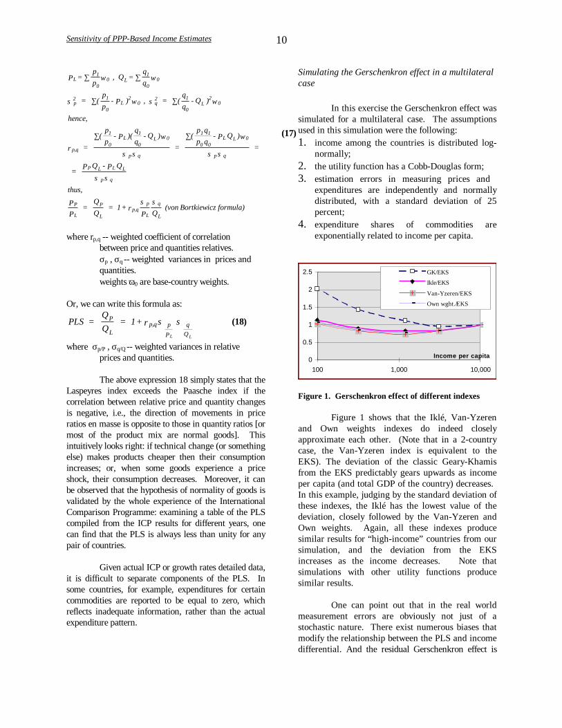
Simulating the Gerschenkron effect in a multilateralcase
In this exercise the Gerschenkron effect wassimulated for a multilateral case. The assumptionsused in this simulation were the following:1. income among the countries is distributed log-
normally;2. the utility function has a Cobb-Douglas form;3. estimation errors in measuring prices and
expenditures are independently and normallydistributed, with a standard deviation of 25percent;
4. expenditure shares of commodities areexponentially related to income per capita.
0
0.5
1
1.5
2
2.5
100 1,000 10,000
Income per capita
GK/EKS
Ikle/EKS
Van-Yzeren/EKS
Own wght./EKS
Figure 1. Gerschenkron effect of different indexes
Figure 1 shows that the Iklé, Van-Yzerenand Own weights indexes do indeed closelyapproximate each other. (Note that in a 2-countrycase, the Van-Yzeren index is equivalent to theEKS). The deviation of the classic Geary-Khamisfrom the EKS predictably gears upwards as incomeper capita (and total GDP of the country) decreases. In this example, judging by the standard deviation ofthese indexes, the Iklé has the lowest value of thedeviation, closely followed by the Van-Yzeren andOwn weights. Again, all these indexes producesimilar results for “high-income” countries from oursimulation, and the deviation from the EKSincreases as the income decreases. Note thatsimulations with other utility functions producesimilar results.
One can point out that in the real worldmeasurement errors are obviously not just of astochastic nature. There exist numerous biases thatmodify the relationship between the PLS and incomedifferential. And the residual Gerschenkron effect is
Sensitivity of PPP-Based Income Estimates 11
not readily distinguishable in the “democratic”Generalized Geary-Khamis case, i.e. for the Iklé, Van-Yzeren and Own weights (see Appendix, Figure 1),because of the randomly [and systematically] distributedmeasurement errors. On the other hand, in the Geary-Khamis case, the Gerschenkron effect is clearly visible.
The PLS and income per capita
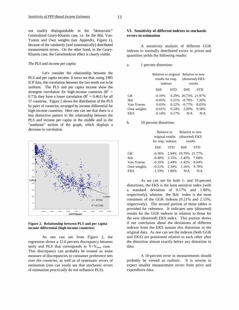
Let's consider the relationship between thePLS and per capita income. It turns out that, using 1985ICP data, the correlation between the two tends not to beuniform. The PLS and per capita income show thestrongest correlation for high-income countries (R2 =0.73); they have a lower correlation (R2 = 0.461) for all57 countries. Figure 2 shows the distribution of the PLSby pairs of countries, arranged by income differential forhigh-income countries. Here one can see that there is aless distinctive pattern to the relationship between thePLS and income per capita in the middle and in the"southeast" section of the graph, which displays adecrease in correlation.
y = .8741e-0.3093x
R^2=0.72850
0.1
0.2
0.3
0.4
0.5
0.6
0.7
0.8
0.9
1
- 0.500 1.000 1.500 2.000 2.500 3.000 3.500 4.000 4.500
ln(Y/Ybase)
1-PLS
Figure 2. Relationship between PLS and per capitaincome differential (high-income countries)
As one can see from Figure 2, theregression shows a 12.6 percent discrepancy betweenunity and PLS that corresponds to Y=Ybase case. This discrepancy can probably be treated as somemeasure of discrepancies in consumer preference setsover the countries, as well as of systematic errors ofestimation (one can easily see that stochastic errorsof estimation practically do not influence PLS).
VI. Sensitivity of different indexes to stochasticerrors in estimation
A sensitivity analysis of different GGKindexes to normally distributed errors in prices andquantities yields the following results:
a. 1 percent distortion:
Relative to original results for resp.
indexes
Relative to new (distorted) EKS
results
Diff. STD Diff. STD
GK -0.19% 0.29% 20.73% 21.97%Ikle -0.05% 0.21% -0.79% 7.26%Van-Yzeren 0.03% 0.22% -0.77% 8.03%Own weights -0.01% 0.24% 2.00% 9.58%EKS -0.14% 0.17% N/A N/A
b. 10 percent distortion:
Relative to original results
for resp. indexes
Relative to new (distorted) EKS
results
Diff. STD Diff. STD
GK -0.36% 2.94% 19.70% 21.77%Ikle -0.40% 2.15% -1.45% 7.68%Van-Yzeren -0.35% 2.44% -1.42% 8.04%Own weights -0.21% 2.34% 1.16% 9.79%EKS -1.19% 1.80% N/A N/A
As we can see for both 1- and 10-percentdistortions, the EKS is the least sensitive index (witha standard deviation of 0.17% and 1.80%,respectively), whereas the Iklé index is the mostconsistent of the GGK indexes (0.21% and 2.15%,respectively). The second portion of these tables isprovided for reference. It indicates new (distorted)results for the GGK indexes in relation to those forthe new (distorted) EKS index. This portion showsif our conclusion about the deviations of differentindexes from the EKS sustain this distortion in theoriginal data. As one can see the indexes (both GGKand EKS) are positioned relative to each other afterthe distortion almost exactly before any distortion indata.
A 10-percent error in measurements shouldprobably be viewed as realistic. It is unwise toexpect smaller measurement errors from price andexpenditure data.
Sensitivity of PPP-Based Income Estimates 12
The above could be expanded to include theerrors in expenditure data that are not independent,in which case the expenditure categories can bemisrepresented due to inconsistencies inspecifications across countries. As for prices, onecan note that the systematic errors (like those inprices of services in low-income countries) influencethe outcome more than the stochastic ones.
VII. Existence and uniqueness for the Iklé procedure
Proofs of existence and uniqueness for theIkle system in this chapter will use some propertiesof the system discussed earlier in this paper. We willshow that the existence and uniqueness of thesolution of the Iklé system follows immediatelyfrom the relation of the Iklé to the Geary-Khamissystem, and from the fact that the Geary-Khamisprocedure is a continuous transformation Ψ withrespect to prices p and quantities q (with respect toquantities it is a continuous monotonously increasingtransformation limited from above as we think of Qas a share in “world” output), and it has a uniquesolution14. This proof can be seen also as acomputational algorithm for solving the Iklé system. In fact, it is useful to use this algorithm tocheck both other Iklé and Geary-Khamisalgorithmae simultaneously.
Let us start with some sets of prices p ji and
quantities q ji . We know that there exists a unique
Geary-Khamis solution for these sets. We will showthat certain transformation of q j
i will yield a Geary-Khamis prices that is equal to the Iklé prices for theoriginal q j
i . Let us write:
Q q q qj j ji
i ji
ji
i= ⋅ = ⋅∑Ψ Π( ,( ) ) ( ,( ) ) (19) is
the Geary-Khamis solution for quantities q ji , prices
are assumed to be constant; Πi(qji,(.)) - are Geary-
Khamis prices (throughout this chapter).
Let’s introduce the following transformation ofquantities q j
i :
q q Qji N
ji N
jN= − −1 1/ (20)
14 See, Khamis (1970), Rao (1971) for proofs ofexistence and uniqueness for the solution to the Geary-Khamis system.
Iterations to arrive at the Ikle solution will consist ofestimating consecutive GK solutions for each q j
i N :
Q q qq
Q
q
Qj
Ni j
i N
iji N
iji N
jN
i
ji N
jN= ⋅ = ⋅
∑ ∑
−
−
−
−Π Π( ,( )) ,( )1
1
1
1
Without restricting generality we can assume that
Q MjN
j
M
=∑ =
1. We will prove that lim
N ji N
ji Nq q
→ ∞
−= 1,
or, equivalently, limN j
NQ→ ∞
= 1.
Let us rewrite (20) as: q q Qji N
ji
L
N
jL=
=
−( ) /0
1
1Π
Then, substituting it in expression (19), we obtain
Π ΠL
N
jL
i ji N
ji
iQ q q
== ⋅∑
0
0( ,( ) )
( ), which is limited
from above and below.We will rewrite two consecutive Q j
L+ 1and Q jL as
follows:
1
1
= ⋅
= ⋅
∑
∑+
Π
Π
i ji L j
i L
jL
i
jL
iji L
jL
ji L
jL
i
Q
Q
q
Q
( ,( ) )
( ,( ) )
(21)
It follows from here that Ln Q Ln QjL
jL( ) ( )+ <1 ,
because εΠi ji
j
q
Q
( ) - the elasticity of Q j on
international prices Πi jiq( ,( ) )⋅ due to changes in
q ji - is less than unity in absolute value15. This
means that each iteration produces smaller changes
in ΠL
N
jLQ
=0 than the previous one, and because
15 One can easily show that
ε ω εΠΠ
i ji
j
jii
ji
iq( )
= <∑ 1 (21a),
because | |εq ji
iΠ < 1 . Here εq ji
iΠ stands for the elasticity of
Πi jiq( ,( ) )⋅ on quantities q qj
iji
j= ( )0 ζ , where ζ j is a
scalar.

Sensitivity of PPP-Based Income Estimates 13
Ln Q Ln QL
N
jL
L
N
jLΠ Σ
= =
=
0 0( ) has a limit16 we get
limN
jNQ
→ ∞= 1 .
Thus, we can writelim lim ( ,( ) )L j
L
L i ji L
ji L
iQ q q
→ ∞ → ∞= ⋅ =∑ Π 1, which is the
solution for a Geary-Khamis system with~ lim /
( )q q Qj
i
Lji
N
L
jN=
→ ∞ =
0
1Π . Then, using expression (12)
we can say that international prices Πi jiq(~ ,( ) )⋅ are
the Iklé international prices both for the original setq j
i and for the transformed set ~q ji (because under the
Iklé system, international prices are determined by
expenditure structures ω ji i j
i
i ji
i
q
q= ∑
ΠΠ
) and, in turn,
correspond to the Geary-Khamis international prices
for the transformed set ~ lim /( )
q q Qji
Lji
N
L
jN=
→ ∞ =
0
1Π .
Weights in the Iklé system in this case are
ω ji j
i
LjL
jiq
Q
q= =
→ ∞
~
lim
~
1. Thus, we can write that
Q Q q q
q
q Q q
jIkle
L N
L
jN
i ji
ji
i
i L
ji
N
L
jN
ji
i
i ji
jIkle
ji
i
= = ⋅ =
=
⋅
=
= ⋅
→ ∞ =
→ ∞
=
∑
∑
∑
lim (~ ,( ) )
lim ,( )
( / ,( ) )
( )
( )( )
( ) ( )
Π Π
ΠΠ
Π
0
0
0
0
0
0 0
(22)
and, thus, the iterations converge to a uniquesolution, which is the Ikle solution. QED
The above discourse provides a proof ofexistence and uniqueness, as well as an algorithm tosolve the Ikle system. Uniqueness and existencealone can be shown easier:
16 According to D’Alembert’s Test Σ
L
N Lx=0
is convergent
if x
xq
L
L
+
≤ <1
1. On the other hand, if a series is
absolutely convergent (i.e. convergent for moduli) then the
series is convergent. I.e., ∃ finite limL
L
L
x→ ∞ =
∞∑
0
.
PROPOSITION. Solution for the Ikle systemdefined in (10) exists and is unique.
Existence: Consider the following transformationΩ Π( ) ( / ,( ) )Q q Q qj
Ii j
ijI
ji
i= ⋅∑ , again Πi(qj
i,(.)) -
are Geary-Khamis prices, 1
11MQ j
I
j
M
=∑ = . The
solution obviously exists and is unique. Ω ( )Q jI is a
continuous mapping of M-dimensional simplex Q j
I onto itself, henceforth, applying Brouwer’s
Fixed Point Theorem, we have at least one pointwhere Q Qj j
* *( )= Ω . This is the Ikle solution17.
Uniqueness: Assume, we have two Iklesolutions: Q Qj j
* **, . Then, denoting
x Q y Q qji
j ji
j ji* **= = , we can write:
1 = ⋅ = ⋅∑ ∑Π Πi ji
ji
ii j
iji
ix x y y( ,( ) ) ( ,( ) )
and
Q Q y Q Q y
Q Q x Q Q x
j j i ji
j j ji
i
j j i ji
j j ji
i
* ** ** *
** * * **
( ,( ) )
( ,( ) )
= ⋅
= ⋅
∑∑
Π
Π
Q Qj j* **/ and 1 are Ikle solutions for quantities yj
i,
Q Qj j** */ and 1 are Ikle solutions for quantities xj
i.
This would involve Q Q Q Q Mj jj
j jj
** * * **∑ ∑= = ,
which, for positive Q Qj j* **, , is possible only when
Q Qj j* **≡ 18. QED
VIII. Implementation of alternative aggregationprocedures
17 In a way, previous proof can be seen as a computationalrealization of Brouwer’s FPT for this system (compare itwith equation (22)).
18 In fact, the elasticity consideration of expression (21a)can be applied here as well: one can consider movingbetween Ikle solutions 1 to Q Qj j
* **/ for quantities yji,
which would require εΠ i ji
j
q
Q
( )=1 : a contradiction.

Sensitivity of PPP-Based Income Estimates 14
In this section, the effect of individualweighting schemes in the Generalized Geary-Khamisframework first discussed. Algorithms solving theGeneralized Geary-Khamis systems were implementedusing environment of Microsoft Excel Visual Basic forApplications. The results of the GGK and some other indexes (11 of them are presented in Figures 1 and 2and Tables 1and 2 of the Appendix) have been used inthis analysis. The PPPs for 56 countries that took partin the 1985 ICP Phase have been estimated for thisexercise (seven Caribbean countries were excluded fromconsideration because of the unreliability of theirresults).
As could be expected from formula (11), theresults shown in Figures 1 and 2 indicate that the Ikléindex approximated both the Van-Yzeren and OwnWeights (the "democratically" modified indexes from(13)). Thus, in our case, the difference between usingweights δj
i and ωji for our aggregation is marginal.
Moreover, even unweighted, the arithmetic meanproduces results approximating both weightedarithmetic means. The GK in its turn deviatessignificantly from these three indexes as could bepredicted. All four Generalized Geary-Khamis indexesare arithmetic mean operators applied to the vector ofrelative prices. The only difference among the four isthe weighting scheme, which leads to a case where thenormalization of weights by columns yields results closeto the unweighted index (Van-Yzeren). Put in otherterms, the variation in normalized weights acrosscountries is considerably less than that of total realexpenditures on the category level. One can see fromFigures 1 and 2 of the Appendix that the Iklé index isnot biased towards the price structure of the high-income countries as the original Geary-Khamis is.
In this investigation, the Geary-Khamismethod was applied directly to 139 basic headings, andno supercountry weighting was used; thus, the GKresults became closer in value to those obtained usingthe bilateral USA-based Laspeyres index (Table 1 ofAppendix). It should be noted that introducing the"super-country weighting" would shift the GK indexcloser to the Iklé and EKS. The introduction of the"fixity principle" would cause a similar shift, but wouldbring about a loss of additivity.
The considerable discrepancies one can seebetween the Iklé and Geary-Khamis indexes stem fromthe fact that in the GK system the high-incomecountries influence the international prices more thanthe low-income countries do. In the Iklé world, it is
only the relative expenditure shares of individualcountries expressed in international currency thatmatter, irrespective of the total GDP in those countries.
To illustrate this point, Figure 3 of theAppendix plots international prices according to variousGGK indexes. We observe that the GK prices arepredictably geared towards the US price structure (onthis graph all international prices are plotted against theUS price background).
Table 2 of the Appendix also explicitly showsthe results of one of the statistical tests for additiveindexes that we introduced (closeness to the EKS). TheGK system predictably displays the highest deviation ofGGK indexes, 20.3 percent; the Ikle displays thesmallest magnitude, 6.3 percent. The other two - Van-Yzeren and Own weights - generate a 7.4 and 8.5percent deviation, respectively. Thus, the test shows thatcompared to other GGK indexes the Ikle minimizes theGerschenkron effect.
A correlation analysis for the indexes19 demonstratesthe following (see Table 2 of Appendix):• the GEKS indexes aggregated from bilateral
Fishers and Törnqvist indexes display the strongestcorrelation (r = 0.9999);
• the Iklé and Own Weights, and the Iklé and Rao
show the same high degree of correlation (r =0.9999);
• in general, equal-weighted GGK indexes ( Iklé,
Van-Yzeren and Own Weights) and the Rao indexare a highly correlated group of indexes (r = 0.9993- 0.9999);
• of all equal-weighted GGK indexes ( Iklé, Van-
Yzeren and Own Weights) and the Rao index, the Iklé index displays the highest correlation with theGEKS (aggregated from both Fishers andTörnqvists) and the EKS (weighted) indexes;
The income levels according to differentindexes are presented in Figures 1 and 2. In general,one can see that all aggregation procedures, with thenotable exception of the Paasche, Laspeyres and Geary-Khamis indexes, yield per capita incomes similar to
19 Logarithms are used here in order to emphasizerelative differences as opposed to absolute ones.

Sensitivity of PPP-Based Income Estimates 15
those of the EKS (Fisher) index. The EKS index hasbeen chosen as the reference point, because being amultilateral Fisher, it is practically devoid of theGerschenkron effect. The GEKS index aggregatedfrom bilateral Törnqvist indexes is shown as well. Aswas mentioned above, the EKS index could be modifiedby introducing weights corresponding to the GDP sizeof the countries (weighted EKS index or EKS(w))20. Correlation analysis shows a very tight correlationbetween the EKS (w) and the Fisher, as well as with theoriginal EKS (see Table 2 of the Appendix). The EKS(w) does not have the selection bias that the EKS has,thereby reflecting some of the transaction equalityproperty.
Finally, one has to mention a data problemthat is generated by the ICP itself: the expenditures andprice data collection are not related to each other. Thisgenerates significant incompatibilities not only betweendifferent countries but between different benchmarkyears for the same country. Moreover, introducingquality adjustment coefficients might create anadditional distortion. This produces significant errors inthe data. We can see this from the example of India andBangladesh: these countries seem not to follow thegeneral pattern in the Paasche-Laspeyres spread. Indianprices for goods were adjusted by coefficients that weretoo large (or services, by ones too low), thereby makingthe Indian price structure closer to that of the high-income countries than it apparently is. WithBangladesh, the reverse occurred. This results insignificantly different rankings for the countriesdepending on what aggregation procedure is used.
Rankings 20 The EKS (w) was realized as an iterationprocedure, with the weights being the GDP of individualcountries in EKS (w) terms:
EKS w Fjk k
j
EKS wEKS w
j
kk( ) ( )
( )( )
=∑
Π
Thus defined “plutocratic” version of the EKS opposes the“democratic” EKS, where all the countries have the sameweight in the formula. However, as it can be seen fromour calculations, the EKS (w) produces results practicallyidentical to those obtained using the regular EKS. Fromthe theoretical point of view, the EKS (w) betters the EKSbecause the former satisfies the insignificance of smallcountry property. Being aggregated from the same Fisherindexes, EKS (w) and EKS share all other majorproperties.
One of the most important issues to deal within international comparisons is that of rankings amongthe countries. All the aggregation procedures discussedhere produce rankings that are substantially differentfrom exchange rate rankings. Yet, there exists a muchstronger internal relationship among all the indexesconstructed on the basis of PPP aggregation proceduresthan between any of the PPP indexes and the exchange-rate-converted index. This is related to the fact that allthe aggregation procedures are applied to the same setof national prices and quantities, but they are aggregatedin different ways.
In this analysis, we used standardizedlogarithmic rankings. One can see that a significantdrawback to using discrete rankings (simple ranks) isthat the same difference in ranks for very disparatedifferences in income level can be assigned. Thenormalization of rankings can allow for thisdrawback21.
Next, to elaborate the rankings they wereconverted to logarithms and standardized.Standardization22 allows us to compare the beginning aswell as the end of the list (the discrete rankings andnormalized nominal rankings have restrictedcomparability at the beginning and the end of the list). For example, the USA is ranked number one accordingto all indexes, which does not mean that the relative andabsolute position of the country with respect to othercountries is not affected by the choice of aggregationprocedure. Again, logarithms emphasize relativedifferences instead of absolute ones. In other words thisintends to emphasize the situation when 10 % deviationat $10,000 level would be comparable with the 10 %deviation at $100 level.
Using these calculations we can now addressthe issue of sensitivity from a different prospective:namely, how different countries react to the applicationof various indexes. The sensitivity of the results fordifferent countries due to the aggregation procedureused is presented in Figure 4. Here, the rankings basedon different aggregation procedures are compared on
21 The normalization procedure used here ascribes100 to the highest income level and 0 to the lowest.
22 The standardization procedure involves thedivision of nominal values over their standard deviation.
Sensitivity of PPP-Based Income Estimates 16
the basis of standard deviation in standardizedlogarithmic rankings (standard deviation is estimatedacross indexes). As one can see, the aggregationprocedures under discussion produce the most coherentresults for OECD and Group II countries. A number ofcountries such as Congo, India, Bangladesh, Nepal,Sierra-Leone and Tanzania display rather unstableresults. All these countries have standard deviations inrankings of 10 or more percent. This possibly tells usthat these countries have problems with their basiccategory data. However, in part, the variation isaccounted for by the differences in aggregationprocedures themselves. If the price structure of acountry is distorted (e.g., the relative commodity pricesare too high), the different aggregation procedures willyield results incorporating this distortion to varyingextent.
We can deduce from these results thatalthough the Ikle, Van-Yzeren and Own weightsindexes all exibit a smaller Gerschenkron effect than theGeary-Khamis does, the Ikle index is superior to otherGGK indexes in all conducted statistical tests (namely,standard deviation from the EKS for the simulated andactual 1985 ICP details, the sensitivity to data errors,and the correlation with the GEKS proceduresaggregated from both Fisher and Törnqvist pairwiseindexes). One can conclude that though the Iklé index does not eliminate the Gerschenkron effect completely,as some residual effect is intrinsically embodied in anyadditive aggregation procedure, it does minimize theinfluence of this effect.
IX. Conclusion
The Geary-Khamis index provides additivity(matrix consistency), but it also displays a significantGerschenkron effect. The EKS index is free from theGerschenkron effect, but it does not deliver additivity. On one hand, additivity is important in comparing priceand expenditure structures across different countries. This property is crucial in comparing, for instance,poverty levels, which is important for operationalpurposes in international organizations engaged indevelopment issues. On the other hand, theGerschenkron effect might significantly distort theincome levels in the developing countries, which aremore sensitive to the results of internationalcomparisons. Thus, from the axiomatic (statistical)point of view, the Iklé index is seen as the most suitableindex for specific purposes of the World Bank and otherinternational organizations that prefer making use of a
single index in their analytical work. The Iklé index(like G-K and EKS) is simple for the algorithmization,it minimizes the Gerschenkron effect (being essentiallythe equal-weighted Geary-Khamis index), and itmaintains additivity (being an additive procedure with aset of international prices).
Sensitivity of PPP-Based Income Estimates 17
Annex I
Some theory of the Fisher Index
Lemma 1. If utility function f(x) is linearhomogeneous, and the constraint is linear, then
yff p
xx =∇)()( .
Proof: Assume that x* is a solution to the utilitymaximization problemmaxxf(x): px≤y, then
λ=∇px*)(f , and **)(*)( xxx ⋅∇= ff because f(x) is
linear homogeneous. Thus, we obtain
yf λλ == **)( pxx , and yf
f pxx =∇*)(*)( .
Lemma 2. Fisher index corresponds to quadraticutility function.
Proof: Consider the following optimization problem- ν(p,y)=maxx 2/1)()( Axxx ′=f : p⋅x≤y. Then,
yff p
xx =∇)()( (see Lemma 1).
And, consequently,AxxAxp
′′=
y.
Selecting two points x1,p1 and x0,p0, we obtain
11
01
1
01
Axx
Axxxp′′
=y
, and 00
10
0
10
Axx
Axxxp′
′=
y.
Finally, taking the ratio of the two and noting thatA=A′, we arrive at
)()(),( 02
12
00
11
11
01
00
10
1
01
0
10102
xx
Axx
Axx
Axx
Axx
Axx
Axxxpxpxxff
yyQ =′
′=′
′
′
′==
. I.e. Q(Fisher)=f.
Lemma 3. The Fisher index can be represented asan additive index with common prices
01 / ppp +Π= .
Proof: Consider the following optimization problem- maxx )(xf : p⋅x≤y, where f(x) is linearhomogeneous. Thus, we can write xx ff ∇=)(
(Euler's Theorem). On the other hand,
pxp
ff =∇ (see Lemma 1).
We, thus, can write:=∇−∇+∇−∇=∇−∇=− 1
01
00
01
10
01
101 xxxxxx ffffffff
=∇−+∇−∇+∇−∇ 01
0
101
10
00
11 )1( xxxxx f
ff
ffff
01
0
010101 )())(( xxx f
fff
ff ∇−−−∇+∇ ,
because 11
01
10
1 xpxpx ff =∇ , and
00
10
01
0 xpxp
x ff =∇ , and
therefore 0
10
1
10
ff
ff =
∇∇
xx .
Or, ))(()1)(( 0101
0
01
01 xxx −∇+∇=∇+− ff
ff
ff , and
)(1
012/1
0101 xx −
+∇+∇=− −PLS
ffff , where
00
10
01
11
)spreadLaspeyresPaasche(xpxp
xpxp=−PLS .
Which translates into )(1
012/101
01 xxpp −
++Π=− −PLS
ff .
Or, written differently, 12/1
011*10
*001 )1)()(( −−+−+=− PLSff xxpp λλ ,
where λ* is marginal utility of income.
Lemma 4. Contributions of individual componentsto the growth expressed by the Fisher index is
001
0101
0
01
)())(()(
xppxxpp
pxxxp
+Π−+Π=−=
iiiii
iC .
Proof: We can express growth as follows:
001
0101
0
0101 )(
))(()(1
xppxxpp
pxxxp
+Π−+Π=−=−ff (see
Lemma 3). Thus, contributions of individualcomponents to the total growth will be written as
001
0101
0
01
)())(()(
xppxxpp
pxxxp
+Π−+Π=−=
iiiiiii
iC .
Sensitivity of PPP-Based Income Estimates 18
References
S.N.Afriat (1977), The Price Index, CambridgeUniversity Press
L. von Bortkiewicz (1922, 1924), Zweck undStructur einer Preisindexzahl, Nordisk StatistiskTidskrift, 1 and 3
C. Clark (1940), The Conditions of EconomicProgress, London: Macmillan
W.E. Diewert (1981), The Economic Theory of IndexNumbers: a Survey, in Essays in the Theory andMeasurements of Consumer Behavior in Honor ofSir Richard Stone, ed. A. Deaton, CambridgeUniversity Press, London
W.E. Diewert (1987), Index Numbers, in The NewPalgrave: Dictionary of Economics, W.W. Norton& Company, New York
M. Gilbert and I. Kravis (1954), An InternationalComparison of National Products and thePurchasing Power of Currencies, Paris: OEEC
P.Hill (1982), Multilateral Measurements ofPurchasing Power and Real GDP, Eurostat
Doris Iklé (1972), A New Approach to the IndexNumber Problem, Quarterly Journal of Economics
Salem H. Khamis (1970), Properties and Conditionsfor the Existence of a New Type of Index Numbers,Sankhya: The Indian Journal of Statistics, Series B.
A.A. Konüs (1924), Ê Âîïðîñó î Íàñòîÿùåì ÈíäåêñåÑòîèìîñòè Æèçíè, Moscow, [The Problem of theTrue Index of the Cost of living, Trans. inEconometrica, 7 (1939)]
I. Kravis, A. Heston, R. Summers (1982), WorldProduct and Income, The Johns Hopkins UniversityPress, Baltimore and London
Y. Kurabayashi and I. Sakuma (1990), Studies inInternational Comparisons of Real Product andPrices, Kinokuniya Company Ltd., Tokyo
OECD (1992), Purchasing Power Parities and RealExpenditures, 1990, Paris
R.A. Pollak (1990), The Theory of the Cost-of-livingIndex, in Price Level Measurement (ed. W.E.Diewert), North-Holland
D.S. Prasada Rao (1971), On the Existence andUniqueness of a New Class of Index Numbers,Sankhya: The Indian Journal of Statistics, Series B.
P.A. Samuelson and S. Swamy (1974), InvariantEconomic Index Numbers and Canonical Duality:Survey and Synthesis, The American EconomicReview, Vol. 64, N. 4
World Bank (1993), Purchasing Power ofCurrencies: Comparing National Incomes UsingICP Data, Washington, D.C.
Sensitivity of PPP-Based Income Estimates Appendix18
ESP
IRL
NZL
HKG
AUT
BELJPN
ITA
GBR
FIN
FRA
SWE
NLDDEU
DNKAUS
LUXNOR
CAN
USA
85.00%
90.00%
95.00%
100.00%
105.00%
40.00 50.00 60.00 70.00 80.00 90.00 100.00
ETH
TZA
MLI
MWI
SLENPL
MDG
BGD
RWA
IND
ZMB
KENBEN
NGA
SEN
ZWEPAK
EGY
CIV
PHI
LKA
CMR
SWZ
MAR
COG
THATUNBWA
TUR
MUS
KOR
POL
IDN
PRTYUG
GRCHUN
ESP
IRL
NZLHKG
AUTBELJPNITAGBR
FINFRA
SWE
NLDDEUDNKAUSLUXNOR CAN
USA
80.00%
90.00%
100.00%
110.00%
120.00%
130.00%
140.00%
150.00%
160.00%
170.00%
180.00%
1.00 10.00 100.00
Fisher
Tornkvist
EKS(weighted)
GK
Ikle
Van-Yzeren
Own weights
Rao
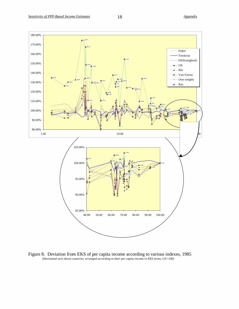
Figure 8. Deviation from EKS of per capita income according to various indexes, 1985(Horizontal axis shows countries arranged according to their per capita income in EKS terms, US=100)

Sensitivity of PPP-Based Income Estimates Appendix19
ESP
IRL
NZL
HKG
AUT
BELJPN
ITA
GBR
FIN
FRA
SWE
NLDDEU
DNKAUS
LUXNOR
CAN
USA
85.00%
90.00%
95.00%
100.00%
105.00%
40.00 50.00 60.00 70.00 80.00 90.00 100.00
ETH
TZA
MLI
MWI
SLENPL
MDG
BGD
RWA
IND
ZMB
KENBEN
NGA
SEN
ZWEPAK
EGY
CIV
PHI
LKA
CMR
SWZ
MAR
COG
THATUNBWA
TUR
MUS
KOR
POL
IDN
PRT
YUGGRC
HUN
ESP
IRL
NZLHKG
AUTBELJPNITAGBR
FIN
FRA
SWE
NLDDEUDNKAUS
LUXNOR CANUSA
80.00%
90.00%
100.00%
110.00%
120.00%
130.00%
140.00%
150.00%
160.00%
170.00%
180.00%
1.00 10.00 100.00
GK
Ikle
Van-Yzeren
Own weights
Figure 9. Deviation from EKS of per capita income according to various additive indexes (GGK),1985
(Horizontal axis shows countries arranged according to their per capita income in EKS terms, US=100)
Sensitivity of PPP-Based Income Estimates Appendix20
0.1
1.0
10.0R
ice
Bre
ad
Mac
aron
i & s
imila
Bee
f & V
eal
Pork
Oth
er fr
esh/
froz
e
Fres
h/fr
ozen
fish
Pres
erve
d/pr
oc'd
Fres
h m
ilk
Che
ese
Eggs
Mar
gari
ne,o
ils &
Dri
ed fr
uit &
nut
Dri
ed/fr
ozen
/pre
Pota
to p
rodu
cts
Cof
fees
Coc
oa
Cho
cola
te &
con
fe
Min
eral
wat
er
Spir
its &
liqu
eur
Bee
r
Oth
er to
bacc
o pr
o
Wom
en's
clot
hing
Clo
th.m
ater
&ac
ces
Men
's fo
otw
ear
Chi
ldre
n's
foot
we
Gro
ss re
nts
Rep
air &
mai
nt.h
o
Gas
Coa
l,fir
ewoo
d&ot
h
Floo
r cov
erin
gs
Hse
hold
text
iles,
Was
hing
app
lianc
e
Hea
t&ai
r-co
nditi
o
Rep
airs
to m
ajor
.
Hou
se c
lean
ing
su
Dom
estic
ser
vice
s
Dru
g, m
edic
al p
re
Ther
apeu
tic a
ppli
Svc
of p
hysi
cian
s
Svc
of n
urse
s
Mot
orcy
cle/
bicy
cl
Mai
nt &
Rep
air s
v
Oth
er p
erso
nal t
r
Long
dis
t.coa
ch/r
Oth
er p
urch
ased
t
Tele
phon
e,te
legr
a
Phot
ogra
phic
eqi
p
Non
-dur
able
rec.
g
Cin
ema,
thea
tre,
sp
Boo
ks, n
ewsp
, pri
Educ
atio
n se
rvic
e
Toile
t art
icle
s
Stat
ione
ry
Staf
f can
teen
s
Fina
ncia
l ser
vice
Res
iden
tial b
ldgs
Bld
gs m
arke
t
Agr
icul
tura
l bld
g
Land
impr
ovem
ent,
Mot
or v
ehic
les
&
Ship
s &
boa
ts
Mac
h.fo
od,c
hem
,pl
Offi
ce e
quip
.pre
c
Equi
p.m
inin
g &
co
Text
ile m
achi
nery
Offi
ce e
quip
.pre
c
Com
pens
. em
ploy
ee
Cha
nge
in s
tock
s
GKIkleVYOW
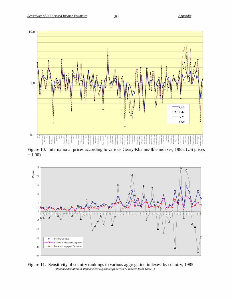
Figure 10. International prices according to various Geary-Khamis-Ikle indexes, 1985. (US prices= 1.00)
-25
-20
-15
-10
-5
0
5
10
15
20
25
USA
CA
N
NO
R
LUX
AU
S
DN
K
DEU
NLD
SWE
FRA
FIN
GB
R
ITA
JPN
BEL
AU
T
HK
G
NZL IR
L
ESP
HU
N
GR
C
YU
G
PRT
IRN
POL
KO
R
MU
S
TUR
BW
A
TUN
THA
CO
G
MA
R
SWZ
CM
R
LKA
PHL
CIV
EGY
PAK
ZWE
SEN
NG
A
BEN
KEN
ZMB
IND
RW
A
BG
D
MD
G
NPL SL
E
MW
I
MLI
TZA
ETH
Perc
ent
STD w/o FisherSTD w/o Paasche&LaspeyresPaasche-Laspeyres Deviation
Figure 11. Sensitivity of country rankings to various aggregation indexes, by country, 1985 (standard deviation in standardized log-rankings across 11 indexes from Table 1)

Sensitivity of PPP-Based Income Estimates Appendix21
Table 1. GDP per capita in International Dollars, 1985
Country EK
S
GK
Ikle
Van
-Yze
ren
Ow
n w
eigh
ts
Rao
Fis
her
Paas
che
Lasp
eyre
s
Torn
kvis
t
EK
S(w
eigh
ted)
Exc
hang
e R
ate
United States 16,786 16,786 16,786 16,786 16,786 16,786 16,786 16,786 16,786 16,786 16,786 16,786 Canada 15,408 15,200 15,143 15,161 15,244 15,170 15,352 15,599 15,109 15,537 15,363 13,805 Norway 13,859 13,769 13,300 13,564 13,663 13,369 13,232 14,736 11,882 13,930 13,324 14,010
Luxembourg 12,953 12,794 12,641 12,866 13,036 12,842 12,650 13,217 12,107 12,953 12,660 9,416 Australia 12,562 12,256 11,983 12,541 12,556 12,217 12,127 13,070 11,252 12,687 12,205 10,648 Denmark 12,448 12,131 11,555 11,507 11,484 11,529 12,030 13,188 10,972 12,386 12,098 11,347 Germany 12,226 11,801 11,225 11,595 11,516 11,348 11,775 12,622 10,985 12,104 11,834 10,147
Netherlands 11,881 11,484 10,840 11,276 11,197 10,977 11,354 11,931 10,806 11,791 11,456 8,901 Sweden 11,861 12,254 11,626 11,168 11,260 11,465 12,111 13,148 11,157 12,041 11,878 12,051 France 11,724 11,597 10,973 11,237 11,296 11,126 11,503 12,540 10,552 11,597 11,550 9,482
Finland 11,314 11,461 11,028 10,769 10,897 10,968 10,971 12,155 9,903 11,357 11,090 11,026 United Kingdom 10,941 10,773 9,880 9,814 9,865 9,888 10,893 11,809 10,049 10,796 10,851 8,072
Italy 10,855 10,886 10,220 10,277 10,321 10,277 10,862 12,056 9,786 10,733 10,735 7,431 Japan 10,839 10,701 10,196 10,586 10,849 10,483 10,113 11,918 8,581 10,462 10,332 11,121
Belgium 10,687 10,509 9,809 9,818 9,910 9,880 10,748 11,450 10,088 10,584 10,619 8,099 Austria 10,584 10,568 9,913 9,798 10,092 10,032 10,592 11,600 9,671 10,422 10,526 8,624
Hong Kong 10,500 10,767 9,426 9,471 9,475 9,462 9,848 12,064 8,039 10,232 10,191 6,142 New Zealand 10,031 10,102 9,684 9,816 10,029 9,825 9,586 11,014 8,342 10,064 9,605 6,865
Ireland 7,111 6,917 6,689 6,681 6,827 6,779 6,935 7,305 6,584 6,996 6,979 5,315 Spain 6,730 6,826 6,306 6,086 6,315 6,342 6,754 7,364 6,194 6,697 6,751 4,301
Hungary 5,720 6,100 5,466 5,369 5,560 5,554 5,790 6,682 5,018 5,794 5,669 1,936 Greece 5,504 5,735 5,210 5,048 5,221 5,232 5,833 6,986 4,870 5,417 5,608 3,366
Yugoslavia 5,086 5,209 4,676 4,665 4,830 4,783 5,249 5,998 4,593 5,062 5,076 2,024 Portugal 4,412 4,624 3,947 3,779 4,005 4,006 4,425 5,583 3,507 4,297 4,351 2,042
Iran 4,292 4,877 4,247 3,993 4,091 4,209 4,385 5,831 3,298 4,307 4,288 3,880 Poland 4,210 4,536 4,211 4,109 4,296 4,282 4,084 4,860 3,433 4,161 4,056 1,908 Korea 3,984 4,189 4,020 3,918 4,114 4,079 3,666 4,691 2,865 3,936 3,758 2,277
Mauritius 3,296 4,418 3,238 3,227 3,348 3,321 3,261 5,284 2,012 3,231 3,169 1,055 Turkey 3,033 3,332 3,127 3,005 3,129 3,142 2,764 3,785 2,019 3,208 2,770 1,049
Botswana 2,696 3,307 2,539 2,486 2,617 2,586 2,704 3,914 1,868 2,650 2,649 1,058 Tunisia 2,472 3,051 2,407 2,311 2,422 2,432 2,475 3,694 1,658 2,449 2,421 1,140
Thailand 2,067 2,575 2,162 2,086 2,204 2,205 2,136 3,470 1,315 2,073 2,036 722 Congo 1,925 2,975 1,916 2,010 2,105 2,048 2,152 3,982 1,163 1,856 1,983 1,115
Morocco 1,781 2,345 1,824 1,701 1,825 1,838 1,758 2,924 1,057 1,829 1,706 584 Swaziland 1,679 1,760 1,430 1,407 1,462 1,449 1,722 2,681 1,106 1,660 1,694 548 Cameroon 1,584 2,112 1,532 1,542 1,569 1,563 1,588 2,494 1,011 1,526 1,549 817 Sri Lanka 1,504 1,968 1,630 1,586 1,687 1,665 1,456 2,654 798 1,550 1,411 384
Philippines 1,480 1,856 1,595 1,494 1,591 1,606 1,348 1,976 919 1,463 1,365 562 Cote d'Ivoire 1,461 1,878 1,334 1,430 1,407 1,382 1,448 2,188 958 1,414 1,418 716
Egypt 1,362 1,876 1,396 1,311 1,416 1,423 1,356 2,473 744 1,350 1,309 746 Pakistan 1,144 1,343 1,031 1,025 1,098 1,081 1,104 1,841 663 1,114 1,095 324
Zimbabwe 1,119 1,334 1,053 1,042 1,067 1,061 1,061 1,517 741 1,114 1,060 538 Senegal 951 1,254 856 908 902 883 1,010 1,676 608 899 974 404 Nigeria 947 1,051 753 795 766 766 890 1,268 624 934 884 973
Benin 794 1,027 768 763 780 780 791 1,297 482 801 764 259 Kenya 722 938 716 675 715 721 699 1,119 436 728 682 303
Zambia 709 1,043 701 698 744 732 771 1,308 455 694 728 334 India 644 715 644 587 638 646 596 819 433 652 599 280
Rwanda 604 898 580 668 658 624 641 1,194 344 568 611 288 Bangladesh 600 1,005 704 719 783 757 678 1,572 292 576 629 135 Madagascar 592 795 581 580 604 598 576 977 339 576 567 286
Nepal 568 996 654 682 755 719 720 1,633 317 533 642 150 Sierra Leone 536 936 568 664 622 604 604 1,304 280 500 561 360
Malawi 443 588 434 437 455 446 425 726 249 439 426 157 Mali 355 462 336 327 346 344 376 640 221 343 357 157
Tanzania 317 401 309 292 317 316 340 495 234 313 323 284 Ethiopia 217 292 207 211 216 212 227 392 131 206 218 110
St. deviation from EKS, % 20.3 6.3 7.4 8.5 7.6 6.1 40.9 14.6 2.3 3.5 23.4
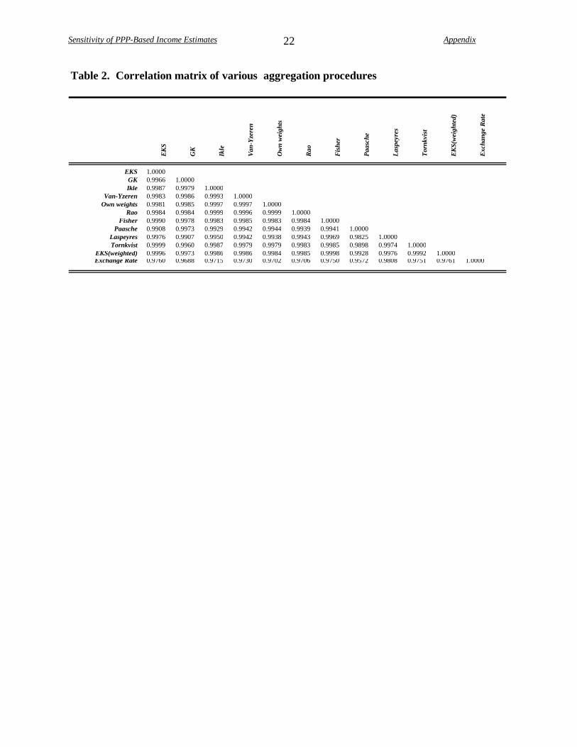
Sensitivity of PPP-Based Income Estimates Appendix22
Table 2. Correlation matrix of various aggregation procedures
EK
S
GK
Ikle
Van
-Yze
ren
Ow
n w
eigh
ts
Rao
Fis
her
Paas
che
Lasp
eyre
s
Torn
kvis
t
EK
S(w
eigh
ted)
Exc
hang
e R
ate
EKS 1.0000GK 0.9966 1.0000Ikle 0.9987 0.9979 1.0000
Van-Yzeren 0.9983 0.9986 0.9993 1.0000Own weights 0.9981 0.9985 0.9997 0.9997 1.0000
Rao 0.9984 0.9984 0.9999 0.9996 0.9999 1.0000Fisher 0.9990 0.9978 0.9983 0.9985 0.9983 0.9984 1.0000
Paasche 0.9908 0.9973 0.9929 0.9942 0.9944 0.9939 0.9941 1.0000Laspeyres 0.9976 0.9907 0.9950 0.9942 0.9938 0.9943 0.9969 0.9825 1.0000Tornkvist 0.9999 0.9960 0.9987 0.9979 0.9979 0.9983 0.9985 0.9898 0.9974 1.0000
EKS(weighted) 0.9996 0.9973 0.9986 0.9986 0.9984 0.9985 0.9998 0.9928 0.9976 0.9992 1.0000Exchange Rate 0.9760 0.9688 0.9715 0.9730 0.9702 0.9706 0.9750 0.9572 0.9808 0.9751 0.9761 1.0000


![[01.08]siteresources.worldbank.org/ICPINT/Resources/270056...section 4, we note that since the median price of the houses sold in each quarter never declined, it is likely that the](https://img.dokumen.tips/doc/110x75/5e42195e0d092f3ec33c258a/0108-section-4-we-note-that-since-the-median-price-of-the-houses-sold-in.jpg)