Sensitivity of compaction-induced multicomponent seismictime shifts to variations in reservoir properties

Steven Shawn Smith1 and Ilya Tsvankin1

ABSTRACT

Pore-pressure variations inside producing reservoirs resultin excess stress and strain that influence the arrival times ofreflected waves. Inversion of seismic data for pressure changesrequires better understanding of the dependence of compaction-induced time shifts on reservoir pressure reduction. Usinggeomechanical and full-waveform seismic modeling, we inves-tigate pressure-dependent behavior of P-, S-, and PS-wave timeshifts from reflectors located above and below a rectangularreservoir embedded in a homogeneous half-space. Our geome-chanical modeling algorithm generates the excess stress/strainfield and the stress-induced stiffness tensor as linear functionsof reservoir pressure. Analysis of time shifts obtained fromfull-waveform synthetic data shows that they vary almostlinearly with pressure for reflectors above the reservoir, but

become nonlinear for reflections from the reservoir or deeperinterfaces. Time-shift misfit curves computed with respectto noise-contaminated data from a reference reservoir fora wide range of pressure reductions display well-defined globalminima corresponding to the actual pressure. In addition, weevaluate the influence of the reservoir width on time shiftsand the possibility of constraining the width using time-lapsedata. We also discuss the impact of moderate perturbations inthe strain-sensitivity coefficients (i.e., third-order stiffnesses)on time shifts and on the accuracy of pressure inversion. Ourfeasibility analysis indicates that the most stable pressure esti-mation from noisy data is provided by multicomponent timeshifts from reflectors below the reservoir. For multicompartmentreservoirs, time shifts can be accurately modeled by linearsuperposition of the excess stress/strains computed for the indi-vidual compartments.

INTRODUCTION

Compaction-induced seismic traveltime shifts can potentially beinverted for pressure and fluid distributions inside a producing res-ervoir. Such an inversion contributes to the understanding of howfluids are moving (sweeping) through a reservoir, of levels of inter-compartment pressure communication, and whether fluid is producedfrom locations away from the wells (Greaves and Fulp, 1987; Landrø,2001; Lumley, 2001; Calvert, 2005; Hodgson et al., 2007; Wikel,2008). Knowledge of reservoir pressure can also be used to estimatestress and strain variations outside the reservoir (Herwanger andHorne, 2005; Dusseault et al., 2007; Scott, 2007). Identifying thosestress patterns helps to guide drilling decisions and reduce the cost ofrepairing or replacing wells snapped or sheared by high stresses.Conventional methodologies employ poststack data and compac-

tion-induced vertical stress/strain to estimate time-lapse velocity

and volume changes (Hatchell and Bourne, 2005; Janssen et al.,2006; Carcione et al., 2007; Hodgson et al., 2007; Roste, 2007; Sta-ples et al., 2007; De Gennaro et al., 2008). However, migration andstacking of data represents a complex filtering process that can cor-rupt phase relationships and arrival times. Further, velocity/strainestimation from field data using this approach often producesresults that disagree with laboratory experiments (Bathija et al.,2009). Also, it has been shown that shear (deviatoric) strains gen-erate significant time shifts, requiring the use of triaxial geomechan-ical interpretation of time-lapse data (Schutjens et al., 2004; Sayersand Schutjens, 2007; Herwanger, 2008; Sayers, 2010; Smith andTsvankin, 2012). Finally, offset dependence of P-wave time shiftsis sensitive to stress-induced anisotropy (Fuck et al., 2009).Estimation of compaction-related time shifts requires geome-

chanical computation of excess strains, strain-induced stiffnesses,and modeling of time-lapse wavefields. Fuck et al. (2009, 2011)

Manuscript received by the Editor 31 August 2012; revised manuscript received 17 April 2013; published online 26 September 2013.1Colorado School of Mines (CSM), Geophysics Department, Center for Wave Phenomena (CWP), Golden, Colorado, USA.

E-mail: SteveSmithCSM@aol.com; ilya@mines.edu.© 2013 Society of Exploration Geophysicists. All rights reserved.

T151

GEOPHYSICS, VOL. 78, NO. 5 (SEPTEMBER-OCTOBER 2013); P. T151–T163, 12 FIGS.10.1190/GEO2012-0361.1

Dow

nloa

ded

10/1

4/13

to 1

38.6

7.12

.93.

Red

istr

ibut

ion

subj

ect t

o SE

G li

cens

e or

cop

yrig

ht; s

ee T

erm

s of

Use

at h

ttp://

libra

ry.s

eg.o

rg/

develop a modeling methodology based on a triaxial strain formu-lation and the nonlinear theory of elasticity, and estimate P-waveshifts using anisotropic ray tracing. Smith and Tsvankin (2012) con-firm the main results of Fuck et al. (2009) and analyze time shifts forS- and PS-waves using finite-difference elastic modeling. Thesestudies demonstrate that volumetric (hydrostatic) and deviatoric(shear) strains generate significant time-shift contributions for allthree (P, S, and PS) modes. According to the results of Smithand Tsvankin (2012), sensitivity of time shifts to reservoir pressurestrongly varies with wave type and reflector location.Here, we use geomechanical and finite-difference seismic mod-

eling to study the dependence of P-, S-, and PS-wave time shifts onreservoir pressure. For a set of reflectors located above and below asingle-compartment reservoir, we evaluate the linearity of timeshifts expressed as a function of reservoir pressure. Time-shift mis-fits with respect to a reference reservoir are examined for a realisticrange of pressure reductions and reservoir widths. We also studythe sensitivity of pressure estimation to noise in the input data andto moderate errors in the third-order stiffness coefficients. We con-clude by analyzing time shifts of P-, S-, and PS-waves for multi-compartment reservoirs.

THEORETICAL BACKGROUND

Modeling traveltime shifts caused by production-inducedchanges in a reservoir is typically treated as a three-step process(Smith and Tsvankin, 2012). First, changes in reservoir parameters(here, pressure reduction) result in excess stress and strain in andaround the reservoir (Figure 1). Second, the excess stress/strain per-turbs the stiffness coefficients (Cij) that govern the velocities andtraveltimes of seismic waves. Third, the stress-induced stiffnessesare used to model time-lapse seismic data and compute the timeshifts between the baseline and monitor surveys. In the tests below,we compute time shifts for the reflectors shown in Figure 2 for a

wide range of pressure reductions and corresponding changes instrain.

Strain, stiffness, and traveltime perturbation

We employ a simplified, 2D rectangular reservoir model afterFuck et al. (2009, 2011) (Figure 1), composed of isotropic Bereasandstone that follows standard Biot-Willis compaction theory(Hofmann et al., 2005; Zoback, 2007). The effective pressure inthe reservoir (Peff ) changes according to a reduction in the porefluid pressure (Pfluid)

ΔPeff ¼ Pc − αPfluid ¼ Pc − α ðξP 0fluidÞ; (1)

where Pc ¼ ρgz is the confining pressure of the overburden, ρ is thedensity of the overburden column, g is acceleration due to gravity, zis reservoir depth, and α is known as the effective stress coefficient(Biot-Willis coefficient for “dry” rock, with air as the only pore in-fill; here, α ¼ 0.85). The coefficient ξ (0 ≤ ξ ≤ 1) expresseschanges in the fluid pressure through its initial value, P 0

fluid, whichcorresponds to a stress/strain equilibrium. Velocities in the modelare reduced by 10% from laboratory-measured values to accountfor differences between static and dynamic stiffnesses in low-porosity rocks (Yale and Jamieson, 1994). Pressure changes occuronly inside the reservoir block.By definition,

α ¼ 1 −Ka

Kg; (2)

where Ka is the aggregate bulk modulus of the material, and Kg isthe bulk modulus of the grains (Zoback, 2007). The value of Ka

varies with pore volume and the pressure-dependent bulk moduliof the pore fluid and matrix (Batzle and Han, 2009; Fjær, 2009).As the material compacts and fluid is removed, the aggregate bulkmodulus of the rock approaches that of the grains (Ka → Kg), and αtends to zero (Hornby, 1996). For the range of pressure/strainchanges used in our studies, we assume uniform fluid type (“deadoil”), such that fluid moduli and Ka remain constant. Also, depres-surization of the reservoir compartment is taken to be uniform.Finally, the material is assumed to remain undamaged and to behavein a linear fashion. Therefore, the value of α in our algorithm staysconstant. However, for cases where compaction-induced changes inthe rock are sufficiently large, α will vary with pressure, porosity, orbulkmoduli. This will make effective pressure changes in equation 1nonlinear in Pfluid.The resulting displacement, stress, and strain changes throughout

the section can be computed from analytic equations discussed byHu (1989), Downs and Faux (1995), and Davies (2003). However,here we perform geomechanical modeling using the finite-element,plane-strain solver from COMSOL (COMSOL AB, 2008), whichhas the ability to handle more complicated, multicompartment res-ervoir geometries. Based on the reduction in the effective pressure,COMSOL computes displacement changes and changes to stressand strain as linear functions of ΔPeff and, in our algorithm, of thefluid pressure Pfluid. The 2.0 km × 0.1 km reservoir is located in a20 km × 10 km model space to obtain stress, strain, and displace-ment close to those for a half-space. Here, we model a single-compartment 2D reservoir, assuming that the reservoir lengthin the X2-direction is large. Reducing the out-of-plane reservoir

P P

P P

P P

Figure 1. Reservoir geometry after Fuck et al. (2009) and Smithand Tsvankin (2012). Pore-pressure (Pp ¼ Pfluid) reduction in-side the reservoir results in an anisotropic velocity field due tothe excess stress and strain. The reservoir is composed of andembedded in homogeneous Berea sandstone (VP ¼ 2300 m∕s,VS ¼ 1640 m∕s, ρ ¼ 2140 kg∕m3) with the following third-orderstiffness coefficients: C111 ¼ −13; 904 GPa, C112 ¼ 533 GPa, andC155 ¼ 481 GPa (Sarkar et al., 2003). The effective stress coeffi-cient α is introduced in equation 1. The coefficient ξ scales fluidpressure with respect to its initial value (see equation 1).

T152 Smith and Tsvankin

Dow

nloa

ded

10/1

4/13

to 1

38.6

7.12

.93.

Red

istr

ibut

ion

subj

ect t

o SE

G li

cens

e or

cop

yrig

ht; s

ee T

erm

s of

Use

at h

ttp://

libra

ry.s

eg.o

rg/

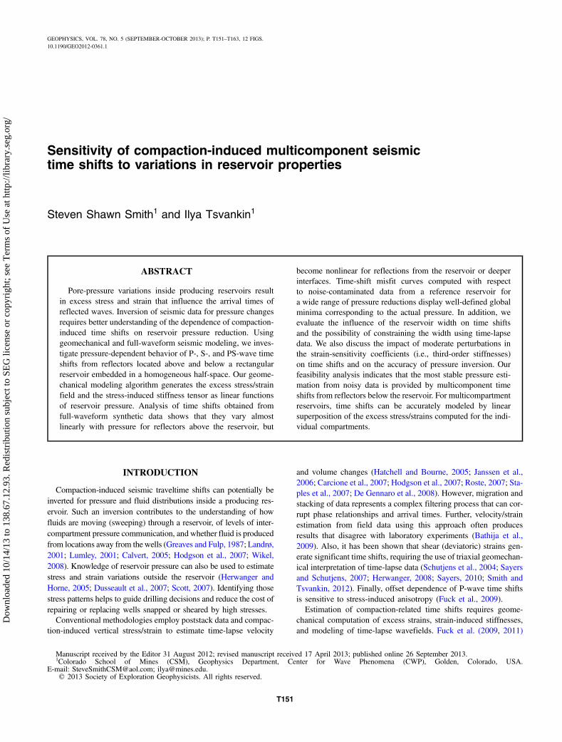
dimensions or adding 3D structure may perturb the in-plane stress/strain field, requiring the use of a 3D geomechanical model. Further,pressure variations inside the reservoir or segmentation of thereservoir volume by faults will require a multicompartment geome-chanical model (an example is discussed below).Typical modeled volumetric and deviatoric strains for the range

of pressures used in our study are shown in Figure 3 for reflector A(Figure 2) and for a horizontal line through the center of the res-ervoir. The volumetric strain (a scalar), which is equal to one-thirdof the trace of the strain tensor, varies linearly with reservoir pres-sure, as expected (Figure 3a). The components of the deviatoricstrain tensor have been summed to illustrate that its variation withpressure reduction is also linear (Figure 3b). The modeled strains inFigure 3 are one or two orders of magnitude higher inside the res-ervoir than in the overburden, and are comparable to those given byBarton (2006) for compacting reservoirs.The strain-induced variations of the stiffness tensor cijkl can be

expressed using the so-called nonlinear theory of elasticity (Hear-mon, 1953; Thurston and Brugger, 1964; Fuck et al., 2009)

cijkl ¼ c0ijkl þ∂cijkl∂emn

Δemn

¼ c0ijkl þ cijklmn Δemn; (3)

where c0ijkl is the second-rank stiffness tensor ofthe background (unperturbed) medium, cijklmn isa sixth-order tensor containing the derivativesof the second-order stiffnesses with respect tostrain, and Δemn is the excess strain tensor.Despite the term “nonlinear,” which applies toHooke’s law, equation 3 expresses the stiffnessescijkl as linear functions of the strainsΔemn. Thus,because the strains Δemn in equation 3 are linearfunctions of the pressure reduction ΔPeff , so arethe second-order stiffnesses cijkl.Wave propagation through the stressed

medium is modeled using Hooke’s law withthe stiffness tensor cijkl. By applying the Voigtconvention, the tensor cijklmn can be convertedinto a matrix Cαβγ , as described by Fuck andTsvankin (2009). For 2D models, we need onlytwo elements of that matrix (C111 and C112), andemploy the values measured on Berea sandstonesamples by Sarkar et al. (2003) (Figure 1). Itshould be noted that measurements of C111

and C112 are rare, and both coefficients are esti-mated with significant uncertainty. For actualreservoir conditions, the coefficients Cαβγ canvary with pressure, temperature, and saturation.Such in situ changes are particularly importantshould α tend toward zero, as this would com-pound variations of the stiffnesses cijkl that de-termine velocity. Here, however, we hold thecoefficients C111 and C112 constant, which keepsthe stiffnesses cijkl linear functions of Δemn andreservoir pressure.While we work with full-waveform data gen-

erated by finite differences, the influence of localstiffness perturbations on time shifts can be

easier understood by analyzing traveltimes computed along rays.Fuck et al. (2011) obtain the P-wave time shifts δt along a certainraypath using a Fermat integral with the integrand linearized in theexcess strains:

Figure 3. Strains generated by geomechanical modeling of a reservoir at 1.5 km depth(Figure 1). (a, b) Volumetric and (c, d) deviatoric strains at (a, c) reflector A and (b, d) ona horizontal line through the center of the reservoir. Legends on each plot indicate hori-zontal distances from the reservoir center (see diamond markers in Figure 2). In this andthe following figures, ΔP is the percentage change in reservoir fluid pressure, which canbe expressed through the coefficient ξ in equation 1 as ΔP ¼ ð1 − ξÞ100.

Figure 2. Reservoir (shaded) and reflectors (marked A, B, and C)used in our study. Strains in Figure 3 are measured at X ¼ 0 km, 1and 2 km on reflector A and on a horizontal line through the res-ervoir center (marked by gray diamonds).

Sensitivity of compaction-induced time shifts T153

Dow

nloa

ded

10/1

4/13

to 1

38.6

7.12

.93.

Red

istr

ibut

ion

subj

ect t

o SE

G li

cens

e or

cop

yrig

ht; s

ee T

erm

s of

Use

at h

ttp://

libra

ry.s

eg.o

rg/

δt ¼ 1

2

Zτ2

τ1

½B1 Δekk þ B2 ðnTΔϵ nÞ� dτ; (4)

where Δekk is the change of the volumetric strain (ekk is 1∕3 of thetrace of strain tensor), Δϵ is the change of the deviatoric straintensor, n is the slowness vector, and

B1 ¼C111 þ 2C112

3C 033

; B2 ¼C111 − C112

C 033

; (5)

where C 033 is the background stiffness coefficient. Equation 4 is

valid only for small stiffness perturbations. The first term of theintegrand in equation 4 corresponds to time shifts due to volumetric(hydrostatic) strains, while the second term accounts for the contri-bution of deviatoric (shearing) strains. Clearly, the time shifts de-scribed by equation 4 are linear in excess strains and, therefore, inthe pressure drop inside the reservoir.In general, however, time shifts are nonlinear in the stiffness

coefficients. Indeed, even the P-wave velocity in a homogeneous,isotropic medium is given by

ffiffiffiffiffiffiffiffiffiffiffiffiC33∕ρ

p, and the traveltime over dis-

tance R is

t ¼ Rffiffiffiffiffiffiffiρ

C33

r. (6)

From equations 4 and 6, we expect time shifts to vary linearly onlyfor small changes in stiffness (ΔCij). Therefore, it is important toevaluate the range of pressure drops, and thus Δemn and ΔCij, forwhich traveltime shifts can be accurately described as linear func-tions of stiffnesses and reservoir pressure. Additional nonlinearity

could be introduced by a pressure/porosity-dependent effectivestress coefficient α (equations 1 and 2) or variations in the coeffi-cients Cαβγ , but such variations are not accounted for by our mod-eling algorithm.The character of the pressure dependence of time shifts from spe-

cific reflectors influences the methodology one would use to invertfor reservoir pressure. Should time shifts vary linearly with reser-voir pressure, estimation of the pressure drop ΔP is possible withstandard linear inversion techniques. Otherwise, it is necessary toemploy a nonlinear/global inversion method.

Time-shift trends versus reflector depth

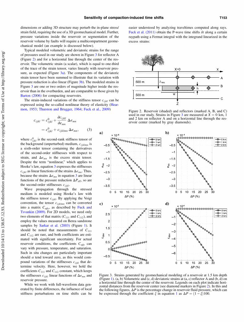
Smith and Tsvankin (2012) use an elastic finite-difference algo-rithm to model P-, S-, and PS-wave reflections for baseline(Pfluid ¼ P 0

fluid) and monitor surveys. Time shifts for each wave typeare computed by isolating specific arrivals in the baseline and mon-itor surveys, computing trace-by-trace crosscorrelations betweenthe surveys, and smoothing the resulting time-shift curves. Figure 4shows typical time-shift surfaces (hulls) for a reservoir at 1.5 kmdepth with a pressure drop of 20%, constructed using data from22 reflectors located between the surface and z ¼ 3 km. For P-waves (Figure 4a), the results are close to those obtained by raytracing (Fuck et al., 2009). Strain-induced P-wave velocityanisotropy around the reservoir causes offset-dependent traveltimeshifts. Laterally varying P-wave time-shift patterns below thereservoir are due to elevated shearing (deviatoric) strains at thereservoir endcaps. The excess strain does not cause substantialSV-wave anisotropy because the resulting symmetry of the mediumis close to elliptical.Time shifts for various wave types/reflector combinations

exhibit different sensitivities to reservoir pressurechanges. For P-waves above and below thereservoir, time shifts vary with offset due tochanging deviatoric stress around the reservoir(Figure 4a). The combination of increased volu-metric and deviatoric strains inside the reservoirgenerates large S- and PS-wave time shifts fromreflectors beneath it (Figure 4b and 4c). Thesetrends provide useful guidance for designing astable pressure-inversion procedure. For thisstudy, reflectors A, B, and C (Figure 2) are usedto measure time shifts of P-, S- and PS-waves fora range of pressure drops and to evaluate the lin-earity of the pressure dependence of time shifts.P-wave time shifts in Figure 4 are somewhat

larger than typical values measured in the field(Guilbot and Smith, 2002; Hatchell and Bourne,2005; Herwanger et al., 2007; Hodgson et al.,2007; Rickett et al., 2007; Staples et al., 2007;De Gennaro et al., 2008). Smaller values ofthe third-order stiffnesses Cαβγ , or a decreasein the effective stress coefficient (α) at largerpressure drops will reduce the magnitude ofmodeled time shifts. However, direct comparisonof our results with time shifts from real-worldreservoirs is nontrivial. In particular, we use lab-oratory data for rock samples with an R-factorthat is much higher than that estimated from fielddata (Hatchell and Bourne, 2005; Bathija et al.,

Figure 4. Typical time-shift surfaces for (a) P-waves, (b) S-waves, and (c) PS-waves,measured using 22 reflectors around the reservoir of Figure 1 (Smith and Tsvankin,2012). The time shifts correspond to hypothetical specular reflection points at each(X; Z) location in the subsurface. Positive shifts indicate lags and negative shifts areleads. Source location is indicated by the white asterisk on top; ΔP ¼ 20%. ReflectorsA, B, and C from Figure 2 are shown for reference.

T154 Smith and Tsvankin

Dow

nloa

ded

10/1

4/13

to 1

38.6

7.12

.93.

Red

istr

ibut

ion

subj

ect t

o SE

G li

cens

e or

cop

yrig

ht; s

ee T

erm

s of

Use

at h

ttp://

libra

ry.s

eg.o

rg/

2009). Also, third-order stiffnesses obtained in a laboratory may notbe suitable for modeling reservoirs without certain adjustment.Complex reservoir models typically incorporate multiple updates

(history matching) of geology and rock-physics properties (strain,velocity, porosity, saturation, temperature, and R-factor) using well-log data (Staples et al., 2007; De Gennaro et al., 2008). Althoughthis approach cannot be implemented here, the spatial patterns inFigure 4 will remain largely unchanged by rock-property updates.For example, the spatial distribution of P-wave time shifts inFigure 4a is similar to that of the time shifts from the Stillwaterfield shown by Staples et al. (2007), despite differences in time-shiftmagnitudes.

METHODOLOGY

Modeling and assumptions

Here, we examine the variation of compaction-induced timeshifts for the three reflectors from Figure 2 due to the pressure dropand the corresponding stiffness change ΔCijðx; zÞ. The initiallyhomogeneous stiffness/velocity field across the section becomesheterogeneous and anisotropic as reservoir pressure is reduced. Fol-lowing geomechanical finite-element modeling of compaction-induced strain [Δemnðx; zÞ], changes in the stiffnesses are computedfrom equation 3. These stiffnesses are used by an elastic finite-difference code (Sava et al., 2010) to generate shot records of re-flected waves.Reflectors A, B, and C are inserted as density perturbations to sam-

ple traveltimes and estimate time shifts for each shot. Then, the multi-component synthetic data are processed to isolate arrivals from thespecific reflector, and time shifts between the reference (baseline) andmonitor reservoir models are computed by crosscorrelation. P-wavetime shifts are measured from the shot records of the vertical displace-ment, while S- and PS-shifts are measured on the horizontal compo-nent. Additional smoothing is applied to reduce time-shift anomaliescaused by interfering arrivals that distort the wavelet shape. For allmodels discussed here, the reservoir depth is 1.5 km, and the source islocated above the center of the reservoir (X ¼ 0).

Misfit (objective) functions

In the tests below, we individually vary reservoir pressure andwidth. Misfits (objective functions) between P-, S-, and PS-wave’stime shifts for a given reservoir ðΔtÞ and reference reservoir modelðΔt refÞ are computed as the L2-norm,

μ ¼ffiffiffiffiffiffiffiffiffiffiffiffiffiffiffiffiffiffiffiffiffiffiffiffiffiffiffiffiffiffiffiffiffiffiffiffiXNk¼1

ðΔt refk − ΔtkÞ2vuut ; (7)

where k ¼ 1; 2; : : : ; N are the individual traces in the shot record.The time-shift misfit between a modeled (test) reservoir and thereference reservoir is calculated by depressurizing both reservoirsfrom the zero-stress/strain initial state. Joint misfit is found asthe L2-norm of the individual wave type misfits,

μjoint ¼ffiffiffiffiffiffiffiffiffiffiffiffiffiffiffiffiffiffiffiffiffiffiffiffiffiffiffiffiμ2P þ μ2S þ μ2PS

q: (8)

Misfits discussed below have not been normalized to facilitate com-parison of results for different wave types at specific reflectors.

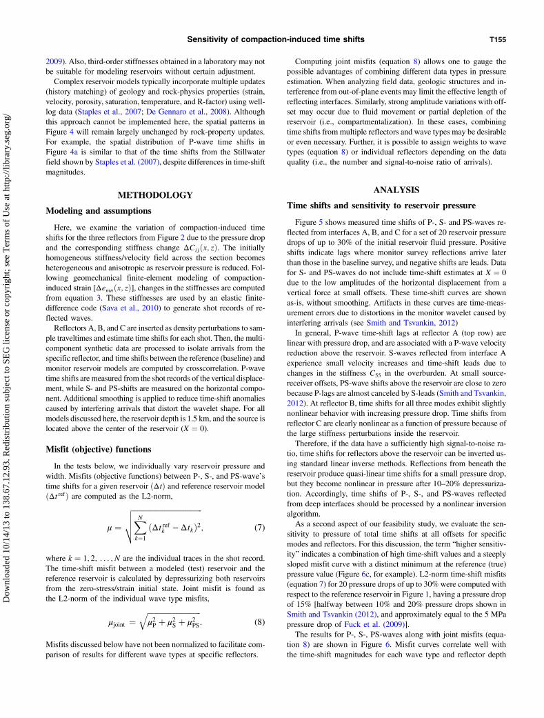
Computing joint misfits (equation 8) allows one to gauge thepossible advantages of combining different data types in pressureestimation. When analyzing field data, geologic structures and in-terference from out-of-plane events may limit the effective length ofreflecting interfaces. Similarly, strong amplitude variations with off-set may occur due to fluid movement or partial depletion of thereservoir (i.e., compartmentalization). In these cases, combiningtime shifts from multiple reflectors and wave types may be desirableor even necessary. Further, it is possible to assign weights to wavetypes (equation 8) or individual reflectors depending on the dataquality (i.e., the number and signal-to-noise ratio of arrivals).

ANALYSIS

Time shifts and sensitivity to reservoir pressure

Figure 5 shows measured time shifts of P-, S- and PS-waves re-flected from interfaces A, B, and C for a set of 20 reservoir pressuredrops of up to 30% of the initial reservoir fluid pressure. Positiveshifts indicate lags where monitor survey reflections arrive laterthan those in the baseline survey, and negative shifts are leads. Datafor S- and PS-waves do not include time-shift estimates at X ¼ 0

due to the low amplitudes of the horizontal displacement from avertical force at small offsets. These time-shift curves are shownas-is, without smoothing. Artifacts in these curves are time-meas-urement errors due to distortions in the monitor wavelet caused byinterfering arrivals (see Smith and Tsvankin, 2012)In general, P-wave time-shift lags at reflector A (top row) are

linear with pressure drop, and are associated with a P-wave velocityreduction above the reservoir. S-waves reflected from interface Aexperience small velocity increases and time-shift leads due tochanges in the stiffness C55 in the overburden. At small source-receiver offsets, PS-wave shifts above the reservoir are close to zerobecause P-lags are almost canceled by S-leads (Smith and Tsvankin,2012). At reflector B, time shifts for all three modes exhibit slightlynonlinear behavior with increasing pressure drop. Time shifts fromreflector C are clearly nonlinear as a function of pressure because ofthe large stiffness perturbations inside the reservoir.Therefore, if the data have a sufficiently high signal-to-noise ra-

tio, time shifts for reflectors above the reservoir can be inverted us-ing standard linear inverse methods. Reflections from beneath thereservoir produce quasi-linear time shifts for a small pressure drop,but they become nonlinear in pressure after 10–20% depressuriza-tion. Accordingly, time shifts of P-, S-, and PS-waves reflectedfrom deep interfaces should be processed by a nonlinear inversionalgorithm.As a second aspect of our feasibility study, we evaluate the sen-

sitivity to pressure of total time shifts at all offsets for specificmodes and reflectors. For this discussion, the term “higher sensitiv-ity” indicates a combination of high time-shift values and a steeplysloped misfit curve with a distinct minimum at the reference (true)pressure value (Figure 6c, for example). L2-norm time-shift misfits(equation 7) for 20 pressure drops of up to 30% were computed withrespect to the reference reservoir in Figure 1, having a pressure dropof 15% [halfway between 10% and 20% pressure drops shown inSmith and Tsvankin (2012), and approximately equal to the 5 MPapressure drop of Fuck et al. (2009)].The results for P-, S-, PS-waves along with joint misfits (equa-

tion 8) are shown in Figure 6. Misfit curves correlate well withthe time-shift magnitudes for each wave type and reflector depth

Sensitivity of compaction-induced time shifts T155

Dow

nloa

ded

10/1

4/13

to 1

38.6

7.12

.93.

Red

istr

ibut

ion

subj

ect t

o SE

G li

cens

e or

cop

yrig

ht; s

ee T

erm

s of

Use

at h

ttp://

libra

ry.s

eg.o

rg/

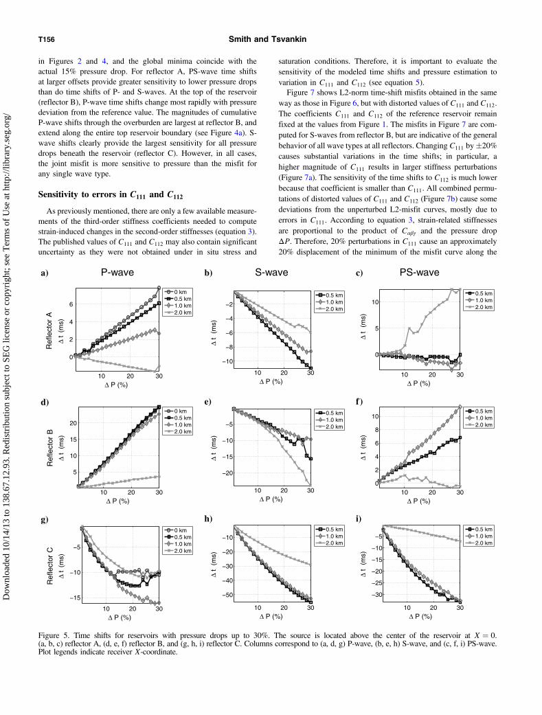
in Figures 2 and 4, and the global minima coincide with theactual 15% pressure drop. For reflector A, PS-wave time shiftsat larger offsets provide greater sensitivity to lower pressure dropsthan do time shifts of P- and S-waves. At the top of the reservoir(reflector B), P-wave time shifts change most rapidly with pressuredeviation from the reference value. The magnitudes of cumulativeP-wave shifts through the overburden are largest at reflector B, andextend along the entire top reservoir boundary (see Figure 4a). S-wave shifts clearly provide the largest sensitivity for all pressuredrops beneath the reservoir (reflector C). However, in all cases,the joint misfit is more sensitive to pressure than the misfit forany single wave type.

Sensitivity to errors in C111 and C112

As previously mentioned, there are only a few available measure-ments of the third-order stiffness coefficients needed to computestrain-induced changes in the second-order stiffnesses (equation 3).The published values of C111 and C112 may also contain significantuncertainty as they were not obtained under in situ stress and

saturation conditions. Therefore, it is important to evaluate thesensitivity of the modeled time shifts and pressure estimation tovariation in C111 and C112 (see equation 5).Figure 7 shows L2-norm time-shift misfits obtained in the same

way as those in Figure 6, but with distorted values of C111 and C112.The coefficients C111 and C112 of the reference reservoir remainfixed at the values from Figure 1. The misfits in Figure 7 are com-puted for S-waves from reflector B, but are indicative of the generalbehavior of all wave types at all reflectors. Changing C111 by�20%

causes substantial variations in the time shifts; in particular, ahigher magnitude of C111 results in larger stiffness perturbations(Figure 7a). The sensitivity of the time shifts to C112 is much lowerbecause that coefficient is smaller than C111. All combined permu-tations of distorted values of C111 and C112 (Figure 7b) cause somedeviations from the unperturbed L2-misfit curves, mostly due toerrors in C111. According to equation 3, strain-related stiffnessesare proportional to the product of Cαβγ and the pressure dropΔP. Therefore, 20% perturbations in C111 cause an approximately20% displacement of the minimum of the misfit curve along the

P-wave

Refl

ecto

rA

10 20 30

0

2

4

6

∆ P (%)

∆ t

(ms)

0 km0.5 km1.0 km2.0 km

a) S-wave

10 20 30

−10

−8

−6

−4

−2

∆ P (%)

∆ t

(m

s)

0.5 km1.0 km2.0 km

b) PS-wave

10 20 30

0

5

10

∆ P (%)

∆ t

(m

s)

0.5 km1.0 km2.0 km

c)

d) e) f)

g) h) i)

Refl

ecto

rB

10 20 30

5

10

15

20

∆ P (%)

∆ t

(ms)

0 km0.5 km1.0 km2.0 km

10 20 30

−20

−15

−10

−5

∆ P (%)

∆ t

(ms)

0.5 km1.0 km2.0 km

10 20 300

2

4

6

8

10

∆ P (%)

∆ t

(ms)

0.5 km1.0 km2.0 km

Refl

ecto

rC

10 20 30

−15

−10

−5

∆ P (%)

∆ t

(ms)

0 km0.5 km1.0 km2.0 km

10 20 30

−50

−40

−30

−20

−10

∆ P (%)

∆ t

(ms)

0.5 km1.0 km2.0 km

10 20 30

−30

−25

−20

−15

−10

−5

∆ P (%)

∆ t

(m

s)

0.5 km1.0 km2.0 km

Figure 5. Time shifts for reservoirs with pressure drops up to 30%. The source is located above the center of the reservoir at X ¼ 0.(a, b, c) reflector A, (d, e, f) reflector B, and (g, h, i) reflector C. Columns correspond to (a, d, g) P-wave, (b, e, h) S-wave, and (c, f, i) PS-wave.Plot legends indicate receiver X-coordinate.

T156 Smith and Tsvankin

Dow

nloa

ded

10/1

4/13

to 1

38.6

7.12

.93.

Red

istr

ibut

ion

subj

ect t

o SE

G li

cens

e or

cop

yrig

ht; s

ee T

erm

s of

Use

at h

ttp://

libra

ry.s

eg.o

rg/

pressure axis (i.e., a 20% increase in C111 is com-pensated by a 20% decrease in ΔP).

Influence of reservoir width

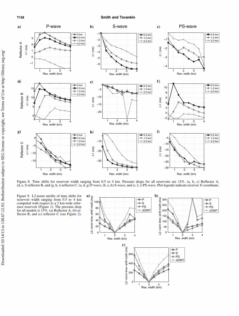
Whereas reservoir depth is typically wellknown from borehole data, the true width ofthe reservoir (or a given reservoir compartment)may be estimated with an error. Because thestress/strain field around the reservoir is a func-tion of the compartment dimensions, the strain-dependent time shifts change with reservoirwidth. In particular, shear (deviatoric) stressesare largest at the endcaps of the reservoir, evenfor reservoirs of elliptical shape (Smith andTsvankin, 2012). The distance between theseshear-strain anomalies varies with reservoirwidth, thus changing the ratio of volumetric todeviatoric strain around the reservoir. An illustra-tion of this variation for multicompartmentreservoirs is shown in Figure 11g and 11h below.Figure 8 displays time shifts of P-, S- and PS-

waves at reflectors A, B, and C for reservoirwidth ranging from 0.5 to 4 km. The referencereservoir width for misfit measurements is 2 km. Time shifts abovereflector A do not vary significantly with reservoir width, exceptwhen shearing strains from the reservoir endcaps are close toone another. However, directly above the reservoir at reflector B,P-wave time shifts change by up to 10 ms. The largest time shiftsoccur for smaller source-receiver offsets at reflector C for wider (ex-ceeding 3 km) reservoirs with ΔP ¼ 15%, reaching magnitudessimilar to those for the reservoir withΔP ¼ 20% shown in Figure 4.The elevated time shifts in the region below the center of wider res-ervoirs (at reflector C) are indicative of a more significant compac-tion within the reservoir (i.e., the ratio of the vertical-to-horizontalstrain inside the reservoir increases with reservoir width). The sen-sitivity curves for P-, S-, and PS-waves (Figure 9) are reasonablysmooth, with the exception of the S-wave misfit for reflector B and areservoir width of 3 km (this is likely due to a processing artifact).As is the case with pressure dependence, joint misfit data from re-flector C are most sensitive to variations in reservoir width.We have also studied the influence of distortions in the stiffnesses

C111 and C112 on the time-shift misfits computed as functions ofreservoir width. As discussed above, the magnitude of time shiftschanges significantly for �20% variation in C111 (less so for var-iations in C112), which results in perturbations for the misfits of allwave types at reflector C (similar to those of the ΔP misfitminima in Figure 7). In particular, the largest shift of the misfit min-imum at reflector C occurs for S-waves, producing a �10%

deviation from the reference value (2 km). Little deviation of themisfit minimum for 20% perturbations to C111 and C112 occursat reflectors A and B. An exception is the misfit curve for S-wavesat reflector A, where the C111 perturbation shifts the misfit mini-mums by up to 50% of the reference width. This is due to compac-tion-induced lateral variations of the stiffness C55 in the overburden(i.e., between the reservoir and the surface). Similar misfit devia-tions do not occur for P-waves at reflector A because significantspatial variations of stiffness C33 take place primarily inside the res-ervoir (Smith and Tsvankin, 2012).

0 10 20 300

100

200

300

400

∆ P (%)

L2−

norm

tim

e−sh

ift m

isfit

(m

s)

UNPERTURBEDC

111 = 20%, C

112 = 0%

C111

= −20%, C112

= 0%

C111

= 0%, C112

= 20%

C111

= 0%, C112

= −20%

a)

b)

0 10 20 300

100

200

300

400

∆ P (%)

L2−

norm

tim

e−sh

ift m

isfit

(m

s)

UNPERTURBEDC

111 = 20%, C

112 = 20%

C111

= −20%, C112

= −20%

C111

= 20%, C112

= −20%

C111

= −20%, C112

= 20%

Figure 7. L2-norm misfits of time shifts for S-waves from reflectorB computed with distorted third-order stiffness coefficients C111and C112. The values of C111 and C112 for the reference reservoir(at ΔP ¼ 15%) are unchanged. The coefficients C111 and C112 aredistorted by �20% (a) independently; (b) simultaneously.

10 20 30

50

100

150

200

250

300

∆ P (%)

L2−

norm

tim

e−sh

ift m

isfit

(m

s)

PSPSJOINT

a) b)

10 20 30

100

200

300

400

∆ P (%)

L2−

norm

tim

e−sh

ift m

isfit

(m

s)

PSPSJOINT

c)

10 20 30

200

400

600

800

∆ P (%)

L2−

norm

tim

e−sh

ift m

isfit

(m

s)

PSPSJOINT

Figure 6. L2-norm misfits of time shifts for reservoir pressure drops ranging from 0% to30%. The reference reservoir corresponds to a pressure drop of 15%. (a) Reflector A,(b) reflector B, and (c) reflector C.

Sensitivity of compaction-induced time shifts T157

Dow

nloa

ded

10/1

4/13

to 1

38.6

7.12

.93.

Red

istr

ibut

ion

subj

ect t

o SE

G li

cens

e or

cop

yrig

ht; s

ee T

erm

s of

Use

at h

ttp://

libra

ry.s

eg.o

rg/

P-wave

Refl

ecto

rA

1 2 3 4

−1

0

1

2

3

Res. width (km)

∆ t

(ms)

0 km0.5 km1.0 km2.0 km

a) S-wave

1 2 3 4

−6

−5

−4

−3

−2

−1

Res. width (km)

0.5 km1.0 km2.0 km

b) PS-wave

1 2 3 4

−4

−3

−2

−1

Res. width (km)

0.5 km1.0 km2.0 km

c)

d) e) f)

g) h) i)

Refl

ecto

rB

1 2 3 4

0

5

10

15

Res. width (km)

0 km0.5 km1.0 km2.0 km

1 2 3 4

−20

−15

−10

−5

Res. width (km)

0.5 km1.0 km2.0 km

1 2 3 4−2

0

2

4

6

8

10

Res. width (km)

0.5 km1.0 km2.0 km

Refl

ecto

rC

1 2 3 4

−15

−10

−5

0

Res. width (km)

0 km0.5 km1.0 km2.0 km

1 2 3 4

−30

−20

−10

Res. width (km)

0.5 km1.0 km2.0 km

1 2 3 4−30

−25

−20

−15

−10

−5

Res. width (km)

0.5 km1.0 km2.0 km

∆ t

(ms)

∆ t

(ms)

∆ t

(ms)

∆ t

(ms)

∆ t

(ms)

∆ t

(ms)

∆ t

(ms)

∆ t

(ms)

Figure 8. Time shifts for reservoir width ranging from 0.5 to 4 km. Pressure drops for all reservoirs are 15%. (a, b, c) Reflector A,(d, e, f) reflector B, and (g, h, i) reflector C. (a, d, g) P-wave, (b, e, h) S-wave, and (c, f, i) PS-wave. Plot legends indicate receiver X-coordinate.

a)

1 2 3 40

50

100

150

200

250

300

Res. width (km)

L2−

norm

tim

e−sh

ift m

isfit

(m

s)

PSPSJOINT

b)

1 2 3 40

200

400

600

Res. width (km)

L2−

norm

tim

e−sh

ift m

isfit

(m

s)

PSPSJOINT

c)

1 2 3 40

20

40

60

80

100

Res. width (km)

L2−

norm

tim

e−sh

ift m

isfit

(m

s)

PSPSJOINT

Figure 9. L2-norm misfits of time shifts forreservoir width ranging from 0.5 to 4 kmcomputed with respect to a 2 km-wide refer-ence reservoir (Figure 1). The pressure dropfor all models is 15%. (a) Reflector A, (b) re-flector B, and (c) reflector C (see Figure 2).

T158 Smith and Tsvankin

Dow

nloa

ded

10/1

4/13

to 1

38.6

7.12

.93.

Red

istr

ibut

ion

subj

ect t

o SE

G li

cens

e or

cop

yrig

ht; s

ee T

erm

s of

Use

at h

ttp://

libra

ry.s

eg.o

rg/

Sensitivity to noise in reference time shifts

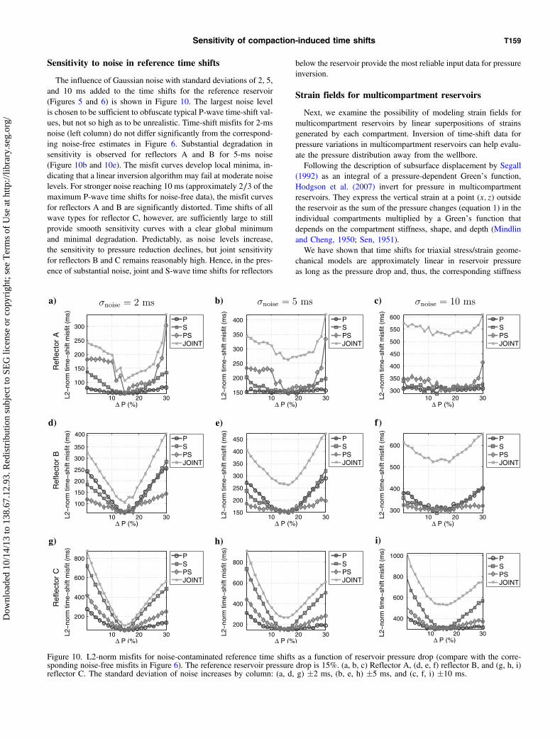
The influence of Gaussian noise with standard deviations of 2, 5,and 10 ms added to the time shifts for the reference reservoir(Figures 5 and 6) is shown in Figure 10. The largest noise levelis chosen to be sufficient to obfuscate typical P-wave time-shift val-ues, but not so high as to be unrealistic. Time-shift misfits for 2-msnoise (left column) do not differ significantly from the correspond-ing noise-free estimates in Figure 6. Substantial degradation insensitivity is observed for reflectors A and B for 5-ms noise(Figure 10b and 10e). The misfit curves develop local minima, in-dicating that a linear inversion algorithm may fail at moderate noiselevels. For stronger noise reaching 10 ms (approximately 2∕3 of themaximum P-wave time shifts for noise-free data), the misfit curvesfor reflectors A and B are significantly distorted. Time shifts of allwave types for reflector C, however, are sufficiently large to stillprovide smooth sensitivity curves with a clear global minimumand minimal degradation. Predictably, as noise levels increase,the sensitivity to pressure reduction declines, but joint sensitivityfor reflectors B and C remains reasonably high. Hence, in the pres-ence of substantial noise, joint and S-wave time shifts for reflectors

below the reservoir provide the most reliable input data for pressureinversion.

Strain fields for multicompartment reservoirs

Next, we examine the possibility of modeling strain fields formulticompartment reservoirs by linear superpositions of strainsgenerated by each compartment. Inversion of time-shift data forpressure variations in multicompartment reservoirs can help evalu-ate the pressure distribution away from the wellbore.Following the description of subsurface displacement by Segall

(1992) as an integral of a pressure-dependent Green’s function,Hodgson et al. (2007) invert for pressure in multicompartmentreservoirs. They express the vertical strain at a point (x; z) outsidethe reservoir as the sum of the pressure changes (equation 1) in theindividual compartments multiplied by a Green’s function thatdepends on the compartment stiffness, shape, and depth (Mindlinand Cheng, 1950; Sen, 1951).We have shown that time shifts for triaxial stress/strain geome-

chanical models are approximately linear in reservoir pressureas long as the pressure drop and, thus, the corresponding stiffness

Refl

ecto

rA

10 20 30

100

150

200

250

300

∆ P (%)

L2−

norm

tim

e−sh

ift m

isfit

(m

s)

PSPSJOINT

a)

10 20 30150

200

250

300

350

400

∆ P (%)

L2−

norm

tim

e−sh

ift m

isfit

(m

s)

PSPSJOINT

b)

10 20 30300

350

400

450

500

550

600

∆ P (%)

L2−

norm

tim

e−sh

ift m

isfit

(m

s)

PSPSJOINT

c)

Refl

ecto

rB

10 20 30

100

150

200

250

300

350

400

∆ P (%)

L2−

norm

tim

e−sh

ift m

isfit

(m

s)

PSPSJOINT

d)

10 20 30150

200

250

300

350

400

450

∆ P (%)

L2−

norm

tim

e−sh

ift m

isfit

(m

s)

PSPSJOINT

e)

10 20 30300

400

500

600

∆ P (%)

L2−

norm

tim

e−sh

ift m

isfit

(m

s)

PSPSJOINT

f)

Refl

ecto

rC

10 20 30

200

400

600

800

∆ P (%)

L2−

norm

tim

e−sh

ift m

isfit

(m

s)

PSPSJOINT

g)

10 20 30

200

400

600

800

∆ P (%)

L2−

norm

tim

e−sh

ift m

isfit

(m

s)

PSPSJOINT

h)

10 20 30

400

600

800

1000

∆ P (%)

L2−

norm

tim

e−sh

ift m

isfit

(m

s)

PSPSJOINT

i)

Figure 10. L2-norm misfits for noise-contaminated reference time shifts as a function of reservoir pressure drop (compare with the corre-sponding noise-free misfits in Figure 6). The reference reservoir pressure drop is 15%. (a, b, c) Reflector A, (d, e, f) reflector B, and (g, h, i)reflector C. The standard deviation of noise increases by column: (a, d, g) �2 ms, (b, e, h) �5 ms, and (c, f, i) �10 ms.

Sensitivity of compaction-induced time shifts T159

Dow

nloa

ded

10/1

4/13

to 1

38.6

7.12

.93.

Red

istr

ibut

ion

subj

ect t

o SE

G li

cens

e or

cop

yrig

ht; s

ee T

erm

s of

Use

at h

ttp://

libra

ry.s

eg.o

rg/

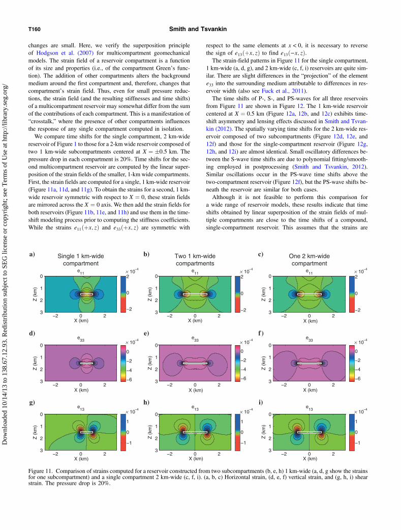
changes are small. Here, we verify the superposition principleof Hodgson et al. (2007) for multicompartment geomechanicalmodels. The strain field of a reservoir compartment is a functionof its size and properties (i.e., of the compartment Green’s func-tion). The addition of other compartments alters the backgroundmedium around the first compartment and, therefore, changes thatcompartment’s strain field. Thus, even for small pressure reduc-tions, the strain field (and the resulting stiffnesses and time shifts)of a multicompartment reservoir may somewhat differ from the sumof the contributions of each compartment. This is a manifestation of“crosstalk,” where the presence of other compartments influencesthe response of any single compartment computed in isolation.We compare time shifts for the single compartment, 2 km-wide

reservoir of Figure 1 to those for a 2-km wide reservoir composed oftwo 1 km-wide subcompartments centered at X ¼ �0.5 km. Thepressure drop in each compartment is 20%. Time shifts for the sec-ond multicompartment reservoir are computed by the linear super-position of the strain fields of the smaller, 1-km wide compartments.First, the strain fields are computed for a single, 1 km-wide reservoir(Figure 11a, 11d, and 11g). To obtain the strains for a second, 1 km-wide reservoir symmetric with respect to X ¼ 0, these strain fieldsare mirrored across the X ¼ 0 axis. We then add the strain fields forboth reservoirs (Figure 11b, 11e, and 11h) and use them in the time-shift modeling process prior to computing the stiffness coefficients.While the strains e11ðþx; zÞ and e33ðþx; zÞ are symmetric with

respect to the same elements at x < 0, it is necessary to reversethe sign of e13ðþx; zÞ to find e13ð−x; zÞ.The strain-field patterns in Figure 11 for the single compartment,

1 km-wide (a, d, g), and 2 km-wide (c, f, i) reservoirs are quite sim-ilar. There are slight differences in the “projection” of the elemente33 into the surrounding medium attributable to differences in res-ervoir width (also see Fuck et al., 2011).The time shifts of P-, S-, and PS-waves for all three reservoirs

from Figure 11 are shown in Figure 12. The 1 km-wide reservoircentered at X ¼ 0.5 km (Figure 12a, 12b, and 12c) exhibits time-shift asymmetry and lensing effects discussed in Smith and Tsvan-kin (2012). The spatially varying time shifts for the 2 km-wide res-ervoir composed of two subcompartments (Figure 12d, 12e, and12f) and those for the single-compartment reservoir (Figure 12g,12h, and 12i) are almost identical. Small oscillatory differences be-tween the S-wave time shifts are due to polynomial fitting/smooth-ing employed in postprocessing (Smith and Tsvankin, 2012).Similar oscillations occur in the PS-wave time shifts above thetwo-compartment reservoir (Figure 12f), but the PS-wave shifts be-neath the reservoir are similar for both cases.Although it is not feasible to perform this comparison for

a wide range of reservoir models, these results indicate that timeshifts obtained by linear superposition of the strain fields of mul-tiple compartments are close to the time shifts of a compound,single-compartment reservoir. This assumes that the strains are

Single 1 km-widecompartment

X (km)

Z (

km)

e11

−2 0 2

0

1

2

3−2

0

2× 10

−4

a) Two 1 km-widecompartments

Z (

km)

e11

−2 0 2

0

1

2

3 −2

0

2× 10

−4 × 10−4

× 10−4 × 10

−4 × 10−4

× 10−4 × 10

−4 × 10−4

b) One 2 km-widecompartment

Z (

km)

e11

−2 0 2

0

1

2

3 −2

0

2

c)

Z (

km)

e33

−2 0 2

0

1

2

3 −6

−4

−2

0

d)

Z (

km)

e33

−2 0 2

0

1

2

3−6

−4

−2

0

e)

Z (

km)

e33

−2 0 2

0

1

2

3−6

−4

−2

0

f )

Z (

km)

e13

−2 0 2

0

1

2

3

−1

0

1

g)

Z (

km)

e13

−2 0 2

0

1

2

3

−1

0

1

h)

Z (

km)

e13

−2 0 2

0

1

2

3

−1

0

1

i)

X (km) X (km)

X (km) X (km) X (km)

X (km) X (km) X (km)

Figure 11. Comparison of strains computed for a reservoir constructed from two subcompartments (b, e, h) 1 km-wide (a, d, g show the strainsfor one subcompartment) and a single compartment 2 km-wide (c, f, i). (a, b, c) Horizontal strain, (d, e, f) vertical strain, and (g, h, i) shearstrain. The pressure drop is 20%.

T160 Smith and Tsvankin

Dow

nloa

ded

10/1

4/13

to 1

38.6

7.12

.93.

Red

istr

ibut

ion

subj

ect t

o SE

G li

cens

e or

cop

yrig

ht; s

ee T

erm

s of

Use

at h

ttp://

libra

ry.s

eg.o

rg/

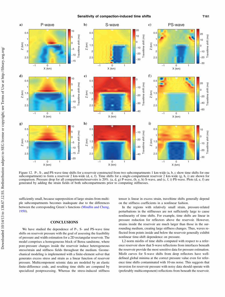
sufficiently small, because superposition of large strains from multi-ple subcompartments becomes inadequate due to the differencesbetween the corresponding Green’s functions (Mindlin and Cheng,1950).

CONCLUSIONS

We have studied the dependence of P-, S- and PS-wave timeshifts on reservoir pressure with the goal of assessing the feasibilityof pressure and width estimation for a 2D rectangular reservoir. Themodel comprises a homogeneous block of Berea sandstone, wherepore-pressure changes inside the reservoir induce heterogeneousstress/strain and stiffness fields throughout the medium. Geome-chanical modeling is implemented with a finite-element solver thatgenerates excess stress and strain as a linear function of reservoirpressure. Multicomponent seismic data are modeled by an elasticfinite-difference code, and resulting time shifts are computed byspecialized postprocessing. Whereas the stress-induced stiffness

tensor is linear in excess strain, traveltime shifts generally dependon the stiffness coefficients in a nonlinear fashion.In the regions with relatively small strain, pressure-related

perturbations in the stiffnesses are not sufficiently large to causenonlinearity of time shifts. For example, time shifts are linear inpressure reduction for reflectors above the reservoir. However,strains inside the reservoir are much larger than those in the sur-rounding medium, creating large stiffness changes. Thus, waves re-flected from points inside and below the reservoir generally exhibitnonlinear time-shift dependence on pressure.L2-norm misfits of time shifts computed with respect to a refer-

ence reservoir show that S-wave reflections from interfaces beneaththe reservoir provide the most sensitive data for pressure estimation.Misfit curves for S-wave shifts from deep reflectors have well-defined global minima at the correct pressure value even for refer-ence time shifts contaminated with 10-ms noise. This suggests thatinversion for reservoir pressure with noisy data should operate with(preferably multicomponent) reflections from beneath the reservoir.

Z (

km)

−1 0 1

0.5

1

1.5

2

2.5 Tra

velti

me

shift

(m

s)

−15

−10

−5

0

5

10

a)

Z (

km)

−1 0 1

0.5

1

1.5

2

2.5 Tra

velti

me

shift

(m

s)

−30

−20

−10

0

10

20

b)

Z (

km)

−1 0 1

0.5

1

1.5

2

2.5 Tra

velti

me

shift

(m

s)

−30

−20

−10

0

10

20

c)

Z (

km)

−1 0 1

0.5

1

1.5

2

2.5 Tra

velti

me

shift

(m

s)

−15

−10

−5

0

5

10d)

Z (

km)

−1 0 1

0.5

1

1.5

2

2.5 Tra

velti

me

shift

(m

s)

−40

−30

−20

−10

0e)

Z (

km)

−1 0 1

0.5

1

1.5

2

2.5 Tra

velti

me

shift

(m

s)

−60

−40

−20

0

20

f )

Z (

km)

−1 0 1

0.5

1

1.5

2

2.5 Tra

velti

me

shift

(m

s)

−20

−15

−10

−5

0

5

10g)

Z (

km)

−1 0 1

0.5

1

1.5

2

2.5 Tra

velti

me

shift

(m

s)

−40

−30

−20

−10

h)

Z (

km)

−1 0 1

0.5

1

1.5

2

2.5 Tra

velti

me

shift

(m

s)

−30

−20

−10

0

10

i)

X (km) X (km) X (km)

X (km) X (km) X (km)

X (km) X (km) X (km)

P-wave S-wave PS-wave

Figure 12. P-, S-, and PS-wave time shifts for a reservoir constructed from two subcompartments 1 km-wide (a, b, c show time shifts for onesubcompartment) to form a reservoir 2 km-wide (d, e, f). Time shifts for a single-compartment reservoir 2 km-wide (g, h, i) are shown forcomparison. Pressure drop for all compartments/reservoirs is 20%. (a, d, g) P-wave, (b, e, h) S-wave, and (c, f, i) PS-wave. Plots (d, e, f) aregenerated by adding the strain fields of both subcompartments prior to computing stiffnesses.

Sensitivity of compaction-induced time shifts T161

Dow

nloa

ded

10/1

4/13

to 1

38.6

7.12

.93.

Red

istr

ibut

ion

subj

ect t

o SE

G li

cens

e or

cop

yrig

ht; s

ee T

erm

s of

Use

at h

ttp://

libra

ry.s

eg.o

rg/

One source of uncertainty in interpretation of time-lapse data isthe strain-sensitivity tensor (i.e., third-order stiffnesses), which ispoorly constrained by existing measurements. Although time shiftsvary substantially with the coefficient C111 (the other coefficient,C112, is much smaller in our model), errors of up to 20% in thethird-order stiffnesses do not alter the general shape of the time-shiftmisfit curves. Still, the minimum misfit moves from the correctpressure value, with the percentage deviation close to the errorin C111.Rock-property differences between laboratory and in situ (i.e.,

from seismic or borehole data) measurements are illustrated bylarge discrepancies between lab- and field-estimated R-factors. Itmay be possible to scale velocities measured on small, dry, low-tem-perature samples in the lab to in situ velocity values. When appliedto reservoir models of the type used here, this may yield modeledtime shifts that are closer to those estimated from field data.Another important parameter that can be potentially estimated

from time shifts is the width of the reservoir. The magnitude of timeshifts increases with reservoir width in a nonlinear fashion. Oursensitivity analysis indicates that, as with pressure estimation, themost reliable information for constraining reservoir width is pro-vided by deep S-wave reflections.Our numerical testing confirms that time shifts for multicompart-

ment reservoirs can be modeled by superposition of the strain fieldsgenerated by the individual compartments. Such linear superposi-tion, however, is valid only when the excess stress/strain is suffi-ciently small. Superposition of the strain-induced time shiftscomputed for each subcompartment is much less accurate becausetime shifts are nonlinear in strain and stiffness.For reservoirs composed of a single or multiple compartments, a

linear inversion method may be sufficient for pressure estimation aslong as pressure changes are small (up to approximately 10%).However, time shifts measured at larger pressure drops shouldbe inverted by a more general, nonlinear (global) algorithm.

ACKNOWLEDGMENTS

We wish to thank the associate editor and reviewers of GEOPHYS-

ICS for helpful comments and suggestions. We are also grateful toRodrigo Fuck (CWP, now HRT-Brazil), Mike Batzle (CSM/CRA),Roel Snieder (CWP), Jyoti Behura (CWP), Matt Reynolds (CUBoulder), Ritu Sarker (CSM/CRA now Shell) for discussions, com-ments, and suggestions, and to Jeff Godwin (CWP, now TransformSoftware) and John Stockwell (CWP) for technical assistance. Thiswork was supported by the Consortium Project on Seismic InverseMethods for Complex Structures at CWP.

REFERENCES

Barton, N., 2006, Rock quality, seismic velocity, attenuation and anisotropy:Taylor & Francis.

Bathija, A. P., M. Batzle, and M. Prasad, 2009, An experimental study of thedilation factor: Geophysics, 74, no. 4, E181–E191, doi: 10.1190/1.3137060.

Batzle, M., and D. Han, 2009, Rock and fluid properties: Seismic rock phys-ics: SEG Continuing Education Series, Denver Geophysical Society.

Calvert, R., 2005, Insights and methods for 4D reservoir monitoring andcharacterization: Distinguished instructor short course: SEG.

Carcione, J. M., M. Landrø, A. F. Gangi, and F. Cavallini, 2007, Determin-ing the dilation factor in 4D monitoring of compacting reservoirs by rock-physics models: Geophysical Prospecting, 55, 793–804, doi: 10.1111/j.1365-2478.2007.00633.x.

COMSOL AB, 2008, COMSOL multiphysics. COMSOL AB, http://www.comsol.com/.

Davies, J. H., 2003, Elastic field in a semi-infinite solid due to thermal ex-pansion of a coherently misfitting inclusion: Journal of Applied Mechan-ics and Technical Physics, 70, 655–660, doi: 10.1115/1.1602481.

De Gennaro, S., A. Onaisi, A. Grandi, L. Ben-Brahim, and V. Neillo, 2008,4D reservoir geomechanics: A case study from the HP/HT reservoirs ofthe Elgin and Franklin fields: First Break, 26, 53–59.

Downs, J., and D. A. Faux, 1995, Calculation of strain distributions in multi-ple-quantum-well strained-layer structures: Journal of Applied Physics,77, 2444–2447, doi: 10.1063/1.358771.

Dusseault, M. B., S. Yin, L. Rothenburg, and H. Han, 2007, Seismic mon-itoring and geomechanics simulation: The Leading Edge, 26, 610–620,doi: 10.1190/1.2737119.

Fjær, E., 2009, Static and dynamic moduli of a weak sandstone: Geophysics,74, no. 2, WA103–WA112, doi: 10.1190/1.3052113.

Fuck, R. F., A. Bakulin, and I. Tsvankin, 2009, Theory of traveltime shiftsaround compacting reservoirs: 3D solutions for heterogeneous anisotropicmedia: Geophysics, 74, no. 1, D25–D36, doi: 10.1190/1.3033215.

Fuck, R. F., and I. Tsvankin, 2009, Analysis of the symmetry of a stressedmedium using nonlinear elasticity: Geophysics, 74, no. 5, WB79–WB87,doi: 10.1190/1.3157251.

Fuck, R. F., I. Tsvankin, and A. Bakulin, 2011, Influence of backgroundheterogeneity on traveltime shifts for compacting reservoirs: GeophysicalProspecting, 59, 78–89, doi: 10.1111/j.1365-2478.2010.00909.x.

Greaves, R. J., and T. J. Fulp, 1987, Three-dimensional seismic monitoringof an enhanced oil recovery process: Geophysics, 52, 1175–1187, doi: 10.1190/1.1442381.

Guilbot, J., and B. Smith, 2002, 4-D constrained depth conversion for res-ervoir compaction estimation: Application to Ekofisk Field: The LeadingEdge, 21, 302–308, doi: 10.1190/1.1463782.

Hatchell, P., and S. Bourne, 2005, Rocks under strain: Strain-induced time-lapse time shifts are observed for depleting reservoirs: The Leading Edge,24, 1222–1225, doi: 10.1190/1.2149624.

Hearmon, R., 1953, ‘Third-order’ elastic coefficients: Acta Crystallographia,6, 331–340, doi: 10.1107/S0365110X53000909.

Herwanger, J., 2008, R we there yet?: 70th Annual International Meeting,EAGE, Extended Abstracts.

Herwanger, J., and S. Horne, 2005, Predicting time-lapse stress effects inseismic data: The Leading Edge, 24, 1234–1242, doi: 10.1190/1.2149632.

Herwanger, J., E. Palmer, and C. R. Schiøtt, 2007, Anisotropic velocitychanges in seismic time-lapse data: 77th Annual International Meeting,SEG, Expanded Abstracts, 26, 2883–2887.

Hodgson, N., C. MacBeth, L. Duranti, J. Rickett, and K. Nihei, 2007,Inverting for reservoir pressure change using time-lapse time strain:Application to Genesis Field, Gulf of Mexico: The Leading Edge, 26,649–652, doi: 10.1190/1.2737104.

Hofmann, R., X. Xu, M. Batzle, M. Prasad, A.-K. Furre, and A. Pillitteri,2005, Effective pressure or what is the effect of pressure?: The LeadingEdge, 24, 1256–1260, doi: 10.1190/1.2149644.

Hornby, B. E., 1996, Experimental investigation of effective stress principlesfor sedimentary rocks: 66th Annual International Meeting, SEG, Ex-panded Abstracts, 1707–1710.

Hu, S. M., 1989, Stress from a parallelepipedic thermal inclusion in a semi-space: Journal of Applied Physics, 66, 2741–2743, doi: 10.1063/1.344194.

Janssen, A. L., B. A. Smith, and G. W. Byerley, 2006, Measuring velocitysensitivity to production-induced strain at the Ekofisk field using time-lapse time-shifts and compaction logs: 76th Annual International Meet-ing, SEG, Expanded Abstracts, 3200–3204.

Landrø, M., 2001, Discrimination between pressure and fluid saturationchanges from time lapse data: Geophysics, 66, 836–844, doi: 10.1190/1.1444973.

Lumley, D., 2001, Time-lapse seismic reservoir monitoring: Geophysics, 66,50–53, doi: 10.1190/1.1444921.

Mindlin, R. D., and D. H. Cheng, 1950, Nuclei of strain in the semi-infinitesolid: Journal of Applied Physics, 21, 926–930, doi: 10.1063/1.1699785.

Rickett, J., L. Duranti, T. Hudson, B. Regel, and N. Hodgson, 2007, 4D timestrain and the seismic signature of geomechanical compaction at Genesis:The Leading Edge, 26, 644–647, doi: 10.1190/1.2737103.

Roste, T., 2007, Monitoring overburden and reservoir changes from prestacktime-lapse seismic data — applications to chalk fields: Ph.D. thesis, Nor-wegian University of Science and Technology.

Sarkar, D., A. Bakulin, and R. L. Kranz, 2003, Anisotropic inversion ofseismic data for stressed media: Theory and a physical modeling studyon Berea sandstone: Geophysics, 68, 690–704, doi: 10.1190/1.1567240.

Sava, P., J. Yan, and J. Godwin, 2010, SFEWE elastic finite difference wave-propagation development code for the Madagascar seismic softwarecollection: http://www.reproducability.org.

Sayers, C. M., 2010, Geophysics under stress: Geomechanical applicationsof seismic and borehole acoustic waves: Distinguished instructor shortcourse: SEG.

Sayers, C. M., and P. M. Schutjens, 2007, An introduction to reservoir geo-mechanics: The Leading Edge, 26, 597–601, doi: 10.1190/1.2737100.

T162 Smith and Tsvankin

Dow

nloa

ded

10/1

4/13

to 1

38.6

7.12

.93.

Red

istr

ibut

ion

subj

ect t

o SE

G li

cens

e or

cop

yrig

ht; s

ee T

erm

s of

Use

at h

ttp://

libra

ry.s

eg.o

rg/

Schutjens, P. M. T. M., T. H. Hanssen, M. H. H. Hettema, J. Merour, P. deBree, J. W. A. Coremans, and G. Helliesen, 2004, Compaction-inducedporosity/permeability reduction in sandstone reservoirs: Data and modelfor elasticity-dominated deformation: SPE Reservoir Evaluation & Engi-neering, SPE 88441, 202–216.

Scott, T. E., 2007, The effects of stress path on acoustic velocities and 4Dseismic imaging: The Leading Edge, 26, 602–608, doi: 10.1190/1.2737101.

Segall, P., 1992, Induced stresses due to fluid extraction from axisymmetricreservoirs: Pure and Applied Geophysics, 139, no. 3/4, 535–560, doi: 10.1007/BF00879950.

Sen, B., 1951, Note on the stresses produced by thermoelastic strain in asemi-infinite elastic solid: Quarterly of Applied Mathematics, 8, 365–369.

Smith, S., and I. Tsvankin, 2012, Modeling and analysis of compaction-induced traveltime shifts for multicomponent seismic data: Geophysics,77, no. 6, T221–T237, doi: 10.1190/geo2011-0332.1.

Staples, R., J. Ita, R. Burrel, and R. Nash, 2007, Monitoring pressuredepletion and improving geomechanical models of the Shearwater fieldusing 4D seismic: The Leading Edge, 26, 636–642, doi: 10.1190/1.2737120.

Thurston, R. N., and K. Brugger, 1964, Third-order elastic constants and thevelocity of small amplitude elastic waves in homogeneously stressed me-dia: Physical Review, 133, A1604–A1610, doi: 10.1103/PhysRev.133.A1604.

Wikel, K. R., 2008, Three-dimensional geomechanical modeling of a tightgas reservoir, Rulison Field, Colorado: M.Sc. thesis, Colorado School ofMines.

Yale, D. P., and W. H. Jamieson, 1994, Static and dynamic mechanicalproperties of carbonates, in P. P. Nelson, and S. E. Laubach, eds., Rockmechanics, models, and measurements challenges from industry: Proceed-ings of the 1st North American Rock Mechanics Symposium, 463–471.

Zoback, M. D., 2007, Reservoir geomechanics: Cambridge University Press.

Sensitivity of compaction-induced time shifts T163

Dow

nloa

ded

10/1

4/13

to 1

38.6

7.12

.93.

Red

istr

ibut

ion

subj

ect t

o SE

G li

cens

e or

cop

yrig

ht; s

ee T

erm

s of

Use

at h

ttp://

libra

ry.s

eg.o

rg/