SENSING SOLUBLE ORGANIC COMPOUNDS WITH MICROBIAL FUEL CELLS

by

Yinghua Feng

B.S., Renmin University of China, 2008

M.S., University of Pittsburgh, 2010

Submitted to the Graduate Faculty of

Swanson School of Engineering in partial fulfillment

of the requirements for the degree of

Doctor of Philosophy

University of Pittsburgh

2012

ii

UNIVERSITY OF PITTSBURGH

SWANSON SCHOOL OF ENGINEERING

This dissertation was presented

by

Yinghua Feng

It was defended on

November 13, 2012

and approved by

Radisav D. Vidic, Ph.D., Professor, Civil and Environmental Engineering Department

Willie F. Harper, Jr., Ph.D., Associate Professor, Civil and Environmental Engineering

Department

Di Gao, Ph.D., Associate Professor, Chemical and Petroleum Engineering Department

Jason D. Monnell, Ph.D., Research Assistant Professor, Civil and Environmental Engineering

Department

Dissertation Director: Willie F. Harper, Jr., Ph.D., Associate Professor, Civil and

Environmental Engineering Department

iii

Copyright © by Yinghua Feng

2012

iv

Water quality is central to the social, economic, and ecological well-beings, so it becomes vital

to monitor aquatic ecosystems. In recent years, multifarious biosensors have demonstrated great

potential to support environmental analysis and water quality monitoring. As one type of

biosensors, microbial fuel cells (MFCs) have been investigated and shown good operational

capabilities. However, the response patterns during MFC-based biosensing process have not

been characterized.

This study explored the start-up, operation, and data analysis associated with an air-

cathode MFC system. Electrical signals were generated in response to the injections of synthetic

water and field samples. The highest coefficient of determination in laboratory testing was

produced when the peak area (PA) was correlated with influent COD concentrations, which is

the approach that has not been previously reported. However, the peaks obtained in field testing

of the MFC were smaller in size and with longer cycle time, and the samples with lower COD

produced smaller peak areas (PAs) and peak heights (PHs). Higher coefficients of determination

(0.99 for synthetic water and 0.95 for field samples) were obtained the artificial neural network

(ANN) model was used for COD determination. Furthermore, the use of ANN permitted

accurate identification of acetate, butyrate, glucose and corn starch.

This study also revealed that addition of BES (2-bromoethane sulfonic acid) increased the

magnitude of peak area (PA) and columbic efficiency (CE) by inhibiting the activity of

methanogens when glucose was used as the primary substrate. A revised ANN was utilized to

SENSING SOLUBLE ORGANIC COMPOUNDS WITH MICROBIAL FUEL CELLS

Yinghua Feng, PhD

University of Pittsburgh, 2012

v

interpret the low concentration peaks and the result showed that ANN processing expanded

detection limits (the lowest linear detectable COD) of MFC biosensor from 20mg/l to a below

5mg /l.

Another properly-trained mathematical model, time series analysis (TSA, at f=0.2)

successfully predicted the temporal current trends in properly functioning MFCs, and in a device

that was gradually failing.

This study was the first MFC biosensing effort to propose peak area as an appropriate

response metric and the first to integrate ANNs and TSA model into MFC-based biosensing.

This study is expected to provide a template for future MFC-based biosensing efforts.

vi

TABLE OF CONTENTS

ACKNOWLEDGEMENTS ..................................................................................................... XII

1.0 INTRODUCTION ........................................................................................................ 1

2.0 LITERATURE REVIEW ............................................................................................ 5

2.1 MICROBIAL FUEL CELLS.............................................................................. 5

2.1.1 History and Typical Operation ...................................................................... 5

2.1.1.1 Air-cathode MFCs................................................................................. 6

2.1.1.2 Aqueous cathode MFCs ........................................................................ 8

2.1.2 Ecology and Metabolism ................................................................................. 9

2.1.2.1 Anode-respiring microorganisms and metabolisms ........................ 10

2.1.2.2 Synergetic microorganisms and metabolisms .................................. 11

2.1.2.3 Competing microorganisms and metabolisms ................................. 13

2.1.3 Extracellular Electron Transfer (EET) Mechanisms ................................. 14

2.1.3.1 Nanowires ............................................................................................ 14

2.1.3.2 Membrane-bound cytochromes ......................................................... 15

2.1.3.3 Soluble mediators ................................................................................ 16

2.1.4 Electrochemical Thermodynamics ............................................................... 16

2.1.5 Sources of Overpotential ............................................................................... 18

vii

2.1.6 MFCs as Biosensors ....................................................................................... 18

2.2 ARTIFICIAL NEURAL NETWORKS ........................................................... 19

2.2.1 Typical Features and Transfer functions .................................................... 20

2.2.2 Development and Training ........................................................................... 22

2.2.3 Using ANNs in Environmental Monitoring................................................. 23

2.3 TIME SERIES ANALYSIS .............................................................................. 24

2.3.1 Typical Features ............................................................................................ 24

2.3.2 Development and Modeling .......................................................................... 25

2.3.3 TSA applications ............................................................................................ 26

2.4 HOMO-LUMO GAP ......................................................................................... 27

3.0 RESEARCH OBJECTIVES ..................................................................................... 28

4.0 MATERIALS AND METHODS .............................................................................. 30

4.1 MICROBIAL FUEL CELL CONFIGURATION AND OPERATION ....... 30

4.2 SYNTHETIC SOLUTION ................................................................................ 33

4.3 ENRICHMENT ................................................................................................. 34

4.4 ANALYTICAL METHODS ............................................................................. 34

4.4.1 Chemical oxygen demand ............................................................................. 34

4.4.2 Columbic efficiency ....................................................................................... 35

4.4.3 Methane measurements ................................................................................ 35

4.5 ELECTROCHEMICAL TESTS ...................................................................... 35

4.6 FIELD TESTING .............................................................................................. 36

4.7 ALGORITHMS DEVELOPMENT ................................................................. 38

4.7.1 Artificial Neural Networks ........................................................................... 38

viii

4.7.2 Times Series Analysis .................................................................................... 41

5.0 RESULTS AND DISCUSSION ................................................................................ 42

5.1 MFC RESPONSES ............................................................................................ 42

5.1.1 Laboratory tests ............................................................................................. 42

5.1.2 Field tests ........................................................................................................ 48

5.1.3 Integration with ANNs .................................................................................. 55

5.2 IDENTIFICATION OF CHEMICALS ........................................................... 63

5.2.1 Systematic Testing ......................................................................................... 63

5.2.2 Random Testing ............................................................................................. 70

5.2.3 Factors Related to Chemical Identification ................................................. 75

5.3 INTEGRATION WITH TSA ........................................................................... 78

5.4 EFFECT OF BES ADDITION ON DETECTION LIMITS.......................... 85

5.4.1 Effect of BES addition on current production ............................................ 85

5.4.2 Effect of BES addition on electron balance ................................................. 86

5.4.3 Integration of ANNs ...................................................................................... 90

6.0 CONCLUSION ........................................................................................................... 92

APPENDIX A .............................................................................................................................. 96

APPENDIX B ............................................................................................................................ 100

APPENDIX C ............................................................................................................................ 103

APPENDIX D ............................................................................................................................ 106

APPENDIX E ............................................................................................................................ 108

BIBLIOGRAPHY ..................................................................................................................... 109

ix

LIST OF TABLES

Table 1. Biosensor examples for determination of compounds and relevant parameters in the environment. ............................................................................................................ 2

Table 2. Regressions obtained from field experiments. ........................................................... 55

Table 3. Response metrics for MFC#1, MFC#2 and MFC#3. ................................................ 56

Table 4. Statistics for 500 training simulations using pseudo steady-state metrics. ............. 58

Table 5. Electron equivalent balance in four MFCs at COD=50mg/l, expressed as COD (mg)................................................................................................................................ 89

x

LIST OF FIGURES

Figure 1. Schematic of Microbial Fuel Cell. ............................................................................... 3

Figure 2. A model for electron transfer. ................................................................................... 10

Figure 3. Artificial neural network schematic. ........................................................................ 20

Figure 4. Schematic of a neuron and the mathematical components..................................... 21

Figure 5. The hyperbolic tangent sigmoid function. ................................................................ 22

Figure 6. Schematic of all investigation objectives in this MFC biosensing study. ............... 29

Figure 7. Schematic diagrams and actual photo of the single-chamber MFCs system used in this study. .................................................................................................................... 32

Figure 8. Four sampling sites in OWC...................................................................................... 37

Figure 9. Schematic of artificial neural network in this study. .............................................. 39

Figure 10. Revised schematic of artificial neural network in substrate identification study...................................................................................................................................... 40

Figure 11. Operating history of MFC #1. ................................................................................. 44

Figure 12. The effect of influent COD on current peak area and current peak height for MFC #1. ..................................................................................................................... 45

Figure 13. Operating history of MFC #2. ................................................................................. 46

Figure 14. The effect of influent COD on current peak area and current peak height for MFC #2. ..................................................................................................................... 47

Figure 15. Operating history of MFC #3. ................................................................................. 49

Figure 16. The effect of influent COD on current peak area and current peak height for MFC #3. ..................................................................................................................... 50

xi

Figure 17. Typical MFC response profile. ................................................................................ 51

Figure 18. Surface water testing for MFC#5. ........................................................................... 52

Figure 19. MFC #2 response, injection of a septic tank sample. ............................................ 53

Figure 20. Normally-distributed current profile (laboratory water sample, 200 mg/L COD)...................................................................................................................................... 57

Figure 21. The relationship between measured and ANN-derived COD concentrations. ... 60

Figure 22. The relationship between actual and ANN-derived values for secondary parameters. ................................................................................................................ 62

Figure 23. Systematic testing results (a)for MFC #1and (b)for MFC #2. .............................. 65

Figure 24. Systematic testing summary. ................................................................................... 67

Figure 25. ANN results in systematic testing. ........................................................................... 69

Figure 26. Random testing result for MFC#1. ......................................................................... 71

Figure 27. Random testing result for MFC #2. ........................................................................ 72

Figure 28. ANN results in random testing. ............................................................................... 74

Figure 29. HOMO-LUMO gap data in MFC#1 and MFC#2.................................................. 77

Figure 30. The effect of training fraction on coefficient of determination. ........................... 79

Figure 31. Training results at f=0.03. ........................................................................................ 80

Figure 32. Training results at f=0.20. ........................................................................................ 81

Figure 33. Temporal current profiles for MFC #1, measurement and modeling. ................ 83

Figure 34. Temporal current profiles for a device requiring maintenance, measurement and modeling. ............................................................................................................ 84

Figure 35. The effect of BES addition on peak area for COD < 50 mg/L. ............................. 87

Figure 36. The effect of BES addition on columbic efficiency for COD < 50 mg/L. ............. 88

Figure 37. ANN correlations for acetate and glucose at COD concentrations less than 50mg/L. ...................................................................................................................... 91

xii

ACKNOWLEDGEMENTS

I am profoundly grateful to my advisor and mentor, Professor Willie Harper, for giving me the

opportunity to work on this fellowship project that is of both fundamental and applied

significances. My doctoral studies under his direction have been an unforgettable journey full of

challenge, inspiration, and reward. The profound knowledge I have gained from Dr. Harper and

the unreserved support I have received are priceless assets for my continued pursuit of a

professional career in environmental engineering and science.

I also thank my Ph.D. committee members: Professors, Radisav Vidic, Di Gao, and Jason

Monnell. They were pleasure to work with and provided me a lot of instrumental guidance and

critiques for the completion of my PhD work.

My studies at Pittsburgh were joyful and productive with the countless interactions and

mutual learning from my student colleagues and laboratory collaborators: Wenjing (Lisa) Cheng,

William Barr, David Sanchez, Bo Niu and Christine Currie.

This study was financial supported by the National Oceanic and Atmospheric

Administration (NOAA), Grant No. NA09NOS4200029. Special thanks go to Frank Lopez and

Dr. David Klarer (Old Woman Creek National Estuary Research Reserve, Huron, OH) for

technical and logistical assistance.

1

1.0 INTRODUCTION

Pollution arising from human activity is causing poor water quality, ecosystem damage, and

negative impacts on human health and local economies (Ayenew and Legesse, 2007; Gupta et

al., 2009; Ghumman, 2011). Pollutants often originate from anthropogenic effluents derived

from urban areas, industry, and agriculture (Singh et al., 2005; Gomes et al., 2011). For example,

leachate from coal combustion wastes affects numerous communities throughout Midwestern

states and dyeing activity is causing water pollution in numerous communities. Hydraulic

fracturing activity is also causing water pollution (Gregory et al., 2011). In order to better

understand and minimize negative impacts, it is vital to monitor the presence of a variety of

pollutants in natural and engineered aquatic systems. There number of initiatives and related

legislative actions is growing in proportion to the rising scientific and social concerns in this area

(Khadka and Khanal, 2008; Kazi et al., 2009; Yerel, 2010; Juahir et al., 2011).

Many biosensors have been investigated to support water monitoring efforts (Riedel et

al., 1988; Kim and Kwon, 1999; Liu and Mattiasson, 2002; Chee et al., 2005; Sara et al., 2006).

Biosensors are defined by the International Union of Pure and Applied Chemistry (IUPAC) as

self-contained integrated devices that are capable of providing specific quantitative or semi-

quantitative analytical information using a biological recognition element (biochemical receptor),

which is retained in direct spatial contact with a transduction element (Sara et al., 2006). They

2

are useful, for example, for the continuous monitoring of a contaminated area. Biosensors offer

the possibility of determining the presence of specific chemicals, or their toxicity. Compared to

conventional analytical methods, biosensors also provide the possibility of portability and

miniaturization.

Biosensors can be used as environmental quality monitoring tools in the monitoring of

both inorganic and organic water pollutants. A wide variety of compounds of environmental

concern can be addressed. Table 1 lists some recent reports on the use of biosensors for different

environmental applications.

Table 1. Biosensor examples for determination of compounds and relevant parameters in the environment.

Biosensor type Biorecognition element

Transducing element

Environmentally relevant compounds

or parameters Features Reference

Optical /Whole-cell

Genetically engineered

bioluminescent bacteria

Bioluminescence Toxicity Portable Lee et al., 2005.

Electrochemical /Whole-cell

Multispecies culture Amperometric Low BOD BODmin=0.088mg/LO2;

BOD/BOD5=0.80 Tan and Wu,

1999.

Optical /Whole-cell

Pseudomonas putida Optical Low BOD

BODmin=0.5mg/L O2; comparison with BOD5:

R2=0.971

Chee et al., 2000.

Electrochemical /DNA

DNA (hybridisation) Chronopotentiometric Chlamydia trachomatis

(DNA)

Previous PCR amplification, LOD: 0.2mg/L

Marrazza et al., 1999.

Optical /Immunochemical Antibodies Fluorescence Propanil (Organic

compounds) LOD: 0.6ng/L Tschmelak et al., 2004.

Electrochemical /Enzymatic Enzyme (AChE) Amperometric

Paraoxon and carbofuran (pesticides)

Discrimination between different AChE

inhibitors by neuronal networks, LOD: 0.2μg/L

Bachmann and Schmid, 1999.

Optical /Whole-cell

Recombinant Escherichia coli Bioluminescence Heavy metals Bioavailable fraction in

soils Liao et al.,

2006. Electrochemical

/Enzymatic Enzymatic Amperometric Inorganic phosphate LOD: 0.57mg/L Parellada et al., 1998.

3

One of the biosensors is a microbial fuel cell (MFC), and these devices have been tested in

water quality monitoring and assessment (Kang et al., 2003; Moon et al., 2004). MFCs consist of

an anode exposed to an electron donor (e.g. an organic pollutant), and a cathode exposed to a

terminal electron acceptor (e.g. oxygen). The two chambers are typically separated by a

permeable membrane. Bacteria grow on the anode, oxidizing organic compounds, and producing

electrons that are transported exogenously to the electrode. The electrons then travel through a

wire (and sometimes across an external resistor) to the cathode, where the terminal electron

acceptor is reduced (Figure 1). Therefore, the presence of soluble organic pollutants should

trigger the generation of current that can be measured and correlated with water quality data.

Figure 1. Schematic of Microbial Fuel Cell.

4

MFCs can be used as biosensors, but the response patterns during MFC-based biosensing

process have not been characterized and there is a need to develop better metrics to improve the

utility of these devices. The overall goal of this study is to improve our understanding of MFC-

based biosensing and develop smart MFC biosensors for water quality monitoring. This work

will involve retrieving performance data for an air-cathode MFC system, exploring quantitative

and qualitative response patterns of MFC-based biosensing.

MFCs have not yet been tested at an estuary, where a lower COD concentration is usually

present. This work will fill this gap by testing MFCs at the Old Woman Creek Estuary in Huron,

OH.

5

2.0 LITERATURE REVIEW

2.1 MICROBIAL FUEL CELLS

2.1.1 History and Typical Operation

MFCs generate current by exploiting the activity of anode-respiring bacteria (ARB) which drive

the process. ARBs grow at the anode by transferring electrons from electron donors (e.g., organic

substrates) to an electrode. MFCs can be operated in batch or continuous mode under a variety of

experimental conditions and with a number of novel architectures. Early work on MFCs

demonstrated that both pure and mixed cultures could generate current, but these experiments

assumed that chemical mediators were required to enable current production (Potter, 1911;

Cohen, 1931). The more recent breakthrough occurred when Kim et al. demonstrated that the

mediator-less operation was feasible and stable (Kim et al., 1999a; Kim et al., 1999b). Now,

MFCs can be configured as a two chamber device (i.e. both anode and cathode submerged in

water), with an air-cathode (i.e. a submerged anode and a cathode exposed to air), as a stack with

anodes and cathodes, or with a biocathode (i.e. with cells that extract electrons from the cathodic

electrode). The air-cathode and two-chamber designs are the most common and are reviewed

here.

6

2.1.1.1 Air-cathode MFCs

Air-cathode MFCs use ambient air to provide the electron acceptor that is required at the anode.

These devices are well-established as suitable MFCs. For example, Liu and Logan (2004) tested

an air-cathode cube MFC that was inoculated with bacteria present in domestic wastewater. They

fed both glucose and raw wastewater as substrates and they discovered that by removing the

proton exchange membrane (PEM) increased the current density in spite of significant oxygen

diffusion into the anode. They also found that the air cathode MFC generally produced current

levels that were significantly greater than those observed from two chamber devices. These

results showed that air cathode MFCs generated more current than two chamber devices and that

the PEM was unnecessary.

Min et al. (2005) also observed an improved electricity generation in an air-cathode

microbial fuel cell by feeding swine wastewater. They fed the same swine wastewater into both

air-cathode MFCs and two-chamber MFCs with an aqueous cathode. They found that a triple

stable current density was achieved in the air-cathode MFC than that from two-chamber devices.

They also found that a COD removal up to 92% and NH4-N removal up to 87% in the animal

wastewater. Their results demonstrated that air-cathode MFCs could utilize animal wastewaters

to generate electricity and simultaneously treat wastewater.

7

Fan et al. (2007) examined the performance of a PEM-less air-cathode microbial fuel

cells. In their experiments, they applied J-cloth layers on the water-facing side of air cathode to

reduce oxygen diffusion to the anode by a lacking of PEM. The MFCs with two-layers of J-cloth

obtained a ≥ 100% increase in columbic efficiency and current density of 0.6mA/cm2. They also

produced 15 times higher power density than those reported for air-cathode MFCs using similar

electrode materials in continuous operational mode. Their study indicated that double J-cloth air-

cathode MFCs prominently increased the feasibility in the practical applications of MFCs for

greatly improvement of the columbic efficiency and power density.

Using brush anodes and tubular cathodes appears to improve the current density of air-

cathode MFCs. For example, Zuo et al. (2007) fed glucose into an air cathode MFC that had a

two tube cathode and a brush anode; the brush was used to create a high-surface-area electrode.

The MFC produced 17.7W/m3 and the power increased when they increased the total surface

area of the tubular cathodes. These results show the performance of a novel modification to the

air-cathode design. Logan et al. (2007) also showed that brush anodes amplify the current density

of air-cathode MFCs with wastewater.

You et al. (2007) tested the performance of a graphite-granule membrane-less tubular air-

cathode microbial fuel cell by continuous operations. They fed glucose into a membrane-less air-

cathode MFC that had a tubular graphite-granule anode (GTMFC). The GTMFC produced a

stable current density of 7.52mA and a very low overall internal resistance of 27Ω, which

generated a high maximum volumetric power of 50.2W/m3. Their results suggested that using a

tubular anode and a membrane-less cathode reduced internal resistance and improved power

generation of sustainable air-cathode MFCs.

8

2.1.1.2 Aqueous cathode MFCs

Two chamber MFCs include an anode chamber separated from the cathode chamber by a cation

exchange membrane (CEM). Most MFCs operate this design with aqueous cathodes with

dissolved oxygen, soluble catholytes or poised potentials (Park and Zeikus, 2003; Bergel et al.,

2005; Oh and Logan, 2005).

Zhang et al. (2006) tested the effect of substrate type on electron recovery in a two-bottle

type MFC with ferricyanide. They fed acetate and glucose into two parallel MFCs after an

inoculation by sedimentary bacteria. They found that acetate-fed MFC generated a higher stable

current generation than that in glucose-fed MFC, and also showed different microbial

communities on the two anodes.

The use of soluble catholytes can improve the current generation compared to systems

using dissolved oxygen at the cathode. For example, Oh et al. (2004) studied the electricity

generation in a two-bottle MFC with a Pt-carbon cathode. The MFC produced a maximum of

0.097mW with dissolved oxygen (saturated) and the maximum power increased by 50-80%

when ferricyanide was utilized. They also found a larger cathode potential for ferricyanide. The

soluble catholytes increase the efficient of electron transfer at the cathode and lower the internal

resistance of the system.

You et al. (2006) examined the current generation with glucose using an H-type two-

chamber MFC. In their experiment, they used different terminal electron accepter at the cathode

and generated a highest power of 116mW/m2 with permanganate catholyte, followed by

26mW/m2 with ferricyanide and 10mW/m2 with dissolved oxygen. They found that the larger

power density was a result of the higher cathode potential.

9

Mohan et al. (2008) also compared the effect of catholyte on bioelectricity generation in a

two-chamber MFC. They separately fed wastewater into two anode media-less MFCs with

aerated cathode and ferricyanide catholyte. The current generation and the COD removal

efficiency increased by 41% and 20% when ferricyanide was catholyte. They also discovered

that an improvement on maximum power yield in the MFC with ferricyanide, respectively. Their

study was consistent with previous studies and also revealed that ferricyanide catholyte could

improve the current generation and helped to remove more substrate compared to systems using

oxygen at the cathode.

In a poised potential experiment, the anode potential can be set at any value using a

potentiostat. Thus, in a MFC with poised penitential, the transfer of those electrons to the anode

surface occurs at a precisely known potential. Bond et al. (2002) poised the potentials in a two-

chamber MFC to examine the electricity generation from marine sediments with

Desulfuromonas acetoxidans and G. metallireducens. They found that 82% and 84% of electrons

were accounted for as current when acetate and benzoate were the substrates.

2.1.2 Ecology and Metabolism

The bacterial communities relevant to MFC operation include anode-respiring bacteria (ARB),

synergetic microorganisms and competing microorganisms. ARBs are responsible for generating

current, synergetic microorganisms interact with ARB, and competing microorganisms may

interfere with current production.

10

2.1.2.1 Anode-respiring microorganisms and metabolisms

ARBs are the microorganisms that can generate an electrical current from organic compounds by

transferring electrons to a solid anode. The most commonly accepted conceptual model for

electron transfer is shown in Figure 2. As ARBs oxidize organic compounds, they harvest

NADH which is then transferred to proteins that are imbedded within the inner membrane. The

energy required to transfer these electrons is partially conserved by the pumping of protons into

the periplasm and then back into the cytoplasm by ATPase. The electron transport chain is

composed of proteins that occupy sequentially higher electrical potentials. Electrons are

ultimately transferred to the surface via a membrane bound protein (as depicted in Figure 2) or

via nanowires. It is also possible for ARBs to transfer electrons to a soluble compound (i.e. a

mediator) that diffuses to the electrode.

Figure 2. A model for electron transfer.

11

The most commonly reported ARB geneses are Geobacter and Shewanella (Logan,

2007); both groups have been recovered from mixed communities and they have been used to

inoculate new devices (Park and Zeikus, 2002; Bond and Lovley, 2003; Li et al., 2011). Recent

research has clarified important metabolic details. Several species of Geobacter and Shewanella

species are well known to use acetate, organic acids and alcohols to generate current (Kim et al.,

2007; Kim and Lee, 2010; Choi and Chae, 2012). Reguera et al. (2006) generated current with

wild type Geobacter sulfurreducens and a mutant that was unable to form pili. They found that

the wild type strain formed thick biofilms that where highly conductive, but the mutant formed

thin biofilms that produced very little current. These results showed that pili are important

electron transfer mechanisms for Geobacter sulfurreducens. Richter et al. (2009) carried out

similar experiments with Geobacter sulfurreducens and mutants that did not have the genes

needed for outer membrane c-type cytochromes (Omc). They found that the proteins OmcZ and

OmcB were both involved in electron transfer. Various species of Shewanella (including

Shewanella putrefaciense and Shewanella oneidensis) have been shown to utilize Omc and pilin

proteins to generate current (Dobbin et al., 1995; Beliaev and Saffarini, 1998; Lower et al., 2001;

Myers and Myers, 2001).

2.1.2.2 Synergetic microorganisms and metabolisms

Fermentation is an energy-yielding process in which organic molecules serve as both the electron

donor and electron acceptor. Fermentation can be carried out by many different groups of

bacteria (e.g. Enterobacter, Serratia, Bacillus and Escherichia) and it is common in both

engineered and natural environments (Tortora et al., 2007). Fermentative microorganisms

12

convert sugars, long chain fatty acids, and proteins into alcohols and volatile fatty acids which

are in turn used by ARBs. Therefore, fermenting microorganisms may cooperate with ARBs

synergistically to generate current when the primary substrates are fermentable. However,

fermenters also generate hydrogen, which is not used by ARBs but is instead used by a

competing group of microorganisms (i.e. methanogens). Therefore, the cooperation between

fermenters and ARBs has been the subject of recent research.

Oh and Logan (2005) treated cereal wastewater by prefermenting the raw wastewater and

then feeding the primary effluent into a single-chamber MFC. Keily et al. (2011) fermented

lignocelluloses and feed a single chamber MFC with the endproducts, and they detected several

groups of ARBs present at the anode. Similar results were obtained from Borole et al. (2009),

who carried out two stage operations for treatment of biorefinary wastewater. These previous

studies established that fermentation and ARB activity may be used together, in spite of the

possibility that hydrogen may be produced.

13

2.1.2.3 Competing microorganisms and metabolisms

Researchers have documented the presence of a variety of specific microbial groups that play a

role in the anaerobic production of methane (Black, 2002). Numerous groups of methanogens

have been identified, including Methanobacterium, Methanobrevibacter, Methanococcus,

Methanosarcina, and Methanothrix (Paul and Diana, 2006). Many methanogens compete

directly with ARBs for one- or two- carbon substrates (such as acetate), while other

methanogenic groups use hydrogen. Therefore, in order to enhance the performance of MFCs,

several studies have studied inhibiting methanogens by exposure to air, heat treatment, acid/base

treatment, and chemical inhibitors (Kim et al., 2004a; Li and Fang, 2007).

Kim et al. (2010) found that lowering the resistance from 600 to 50 Ω reduced the

methanogenic electron loss by 24%. They also inhibited methanogens by adding 2-

bromoethanesulfonate (BES); this strategy increased the columbic efficiency from 35% to 70%.

Oxygen stress also successfully inhibited methanogens, while slightly suppressing the

exoelectrogens, and was believed to be a practical option due to its low operating cost. In

addition, Rittmann et al. (2009) also inhibited methanogens with 50mM of BES and they

observed a 24% increase in the CE.

14

2.1.3 Extracellular Electron Transfer (EET) Mechanisms

ARBs generate current in one of three ways. They may use nanowires, membrane-bound

cytochrome, or soluble mediators to complete extracellular electron transfer (EET). These

electron transfer mechanisms are fundamentally responsible for the current generation observed

in MFCs. It appears that the ability to carry out exogenous electron transfer is widely distributed

among naturally-occurring microorganisms (Bond and Lovely, 2003; Lanthier et al., 2008;

Lovley, 2008).

2.1.3.1 Nanowires

Gorby and Beveridge (2005) first observed the production of the conductive appendages in iron-

reducing bacteria and photosynthetic microorganisms (e.g. phototrophic, oxygenic

cyanobacteria), termed as bacterial “nanowires”. By using conductive scanning tunneling

microscopy, they demonstrated that the appendages were electrically conductive and functioned

as nanowires to transfer electrons from the cell to the surface of electrodes.

Reguera et al. (2005) also similarly reported the production of conductive appendages by

G. sulfurreducens with an atomic force microscope. They found that the structure of nanowires

produced by G. sulfurreducens looked different from those associated with S. oneidensis: the

appendages of G. sulfurreducens appeared relatively thin, but S. oneidensis had thick “cables”,

which might be composed of several conductive wires bundled together.

15

2.1.3.2 Membrane-bound cytochromes

Shewanella and Geobacter are capable of transferring electrons through a chain of c-type

cytochromes across the cell envelope to extracellular electron acceptors (e.g., anodes in MFCs).

Cytochromes are iron-containing electron transfer proteins that are imbedded in the cell

membrane. C-type cytochromes are those that absorb light near a 550 nm wavelength when the

heme iron group is in the reduced (Fe2+) state (Tateo, 1992). C-type cytochromes are nearly

ubiquitous in aerobic microorganisms and very common among facultative and strict anaerobic

groups (Lemberg and Barrett, 1973). Many of the c-type cytochromes are associated with the

outer membrane.

For example, terminal reductases – OmcA and MtrC for S. oneidensis, or OmcE and

OmcS for G. sulfurreducens can either directly transfer electrons to solid extracellular electron

acceptors (anode), or donate electrons to soluble extracellular redox compounds (e.g., humic

compounds, riboflavins) (Rosenbaum et al., 2011).

The genome of G. sulfurreducens contains 111 predicted c-type cytochromes, although

many of them remain uncharacterized (Wei et al., 2010).

16

2.1.3.3 Soluble mediators

It has been widely reported that some soluble mediators added into MFCs resulted in electron

transfer by bacteria (Bond et al., 2002; Logan, 2004; Rabaey and Verstraete, 2005). These

exogenous mediators facilitate EET from the inside of the cell to the outside electrodes.

Common chemical mediators include methyl viologen (MV) (Aulenta et al., 2007; Steinbusch et

al., 2010), anthraquinone-2,6-disulfonate (AQDS) (Hatch and Finneran, 2008), thionin,

potassium ferricyanide (Bond et al., 2002) and neutral red (NR) (Park et al., 1999).

Except for these exogenous mediators above, some endogenous chemical mediators by

Pseudomonas spp. (Venkataraman et al., 2010) or S. oneidensis (Marsili et al., 2008) have also

been reported, such as pyocyain, phenazines or flavins. For example, Rabaey et al. (2005)

investigated a two-chamber MFC primarily containing P. aeruginosa and observed a high

concentration of pyocyanin when electricity was generated in their MFC. They found that

pyocyanin produced by P. aeruginosa also worked for other microorganisms to enhance their

efficiency of electron transfer.

2.1.4 Electrochemical Thermodynamics

Similar to any chemical battery, the electromotive force (or maximum potential), Eemf, in an

MFC can be given by

0 ( )ln( tan )

p

emf r

RT productsE EnF reac ts

= −

17

where E0 is the standard cell electromotive force, R(=8,31447J/mol-K) is the gas

constant, T is the absolute temperature (K), n is the number of electrons transferred, and

F(=96485 C/mol) is Faraday’s constant. All reactions are written in the reduction form.

For anode in MFC, the anode electromotive force (or maximum potential) is expressed as

0 ( )- ln( tan )

p

an an r

RT productsE EnF reac ts

=

Then the cathode electromotive force (or maximum potential) is

0 ( )- ln( tan )

p

cat cat r

RT productsE EnF reac ts

=

In terms of the change in Gibbs free energy (ΔGr), the expression becomes

rGEnF∆

= −

Here, E=Ecat-Ean.

Note here that the reaction is exothermic when ΔGr is negative. Thus, a positive

measured voltage is associated with energy-yielding metabolisms and positive current (due to

Ohm’s Law).

18

2.1.5 Sources of Overpotential

In MFCs, the chemical potential is also influenced by the microbial ecology, the presence and

absence of CEM, and specific catholytes. These processes can result in a difference between the

actual measured potentials and the theoretical maximum open circuit potentials; this difference is

the overpotential.

In electrochemistry, the overpotentials can be caused by activation losses, ohmic losses

and mass transfer losses (Larminie and Dicks, 2000). In MFCs, the activation losses are

predominant and mainly dependent on the current through the electrodes, the surface roughness

and electrochemical characteristics of the electrodes, the mechanism of EET, and the operational

temperature or pressure (Rabaey and Verstraete, 2005). There are many sources of overpotentials

in MFCs, so the potential generated by an MFC is more complicated and difficult to be predicted

than that by a chemical fuel cell. The ohmic losses reflect the resistance to the electrons flows

through the electrodes, as well as the resistance to the ions flow through the electrolyte. Various

MFCs with soluble mediators or catholytes have been discussed and tested to decrease the ohmic

losses (in section 2.1.1.2). Mass transfer losses are caused by the reduction in substrate

concentration during MDFC operation. This is a result of insufficient transportation of reactant to

the electrode surface.

2.1.6 MFCs as Biosensors

There is direct evidence that MFCs can be used as biosensors for water quality monitoring. A

linear relationship between the BOD value and the coulomb produced was observed up to 150

19

ppm in a mediator-less two-chamber microbial fuel cell system (Kim et al., 2003). Chang et al.

(2004) applied a two-chamber microbial fuel cell (MFC) to predict BOD concentrations by the

continuous operation. In their study, a mediator-less microbial fuel cell (MFC) was used as a

biochemical oxygen demand (BOD) sensor in an amperometric mode for real-time wastewater

monitoring. At a hydraulic retention time of 1.05 h, BOD values of up to 100 mg/l were

determined based on a linear relationship. Their results showed that the operations of MFC

biosensors are stable.

Single chamber air-cathode MFCs have also been extensively studied. For example,

Kumlanghan et al. (2007) investigated single-chamber MFCs to produce a cell potential that

correlated well with glucose levels in water samples. Lorenzo et al. (2009) showed that an air

cathode MFC produced a linear relationship between BOD concentration and current output up

to 350 ppm. In their study, they evaluated the performance of an MFC-based biosensor in terms

of its COD range, response time, reproducibility and operational stability with both artificial and

real wastewater. The effect of the reactor volume was also investigated. Their results showed a

linear relationship between current and BOD concentration.

2.2 ARTIFICIAL NEURAL NETWORKS

With the development of computing technology, numerical models are often employed to

simulate water flow and water quality processes to solve specific problems. As one of artificial

intelligence (AI) technologies, Artificial Neural Networks (ANNs) have been integrated into

water quality modeling to analyze engineering problems or environmental problems.

20

2.2.1 Typical Features and Transfer functions

ANNs are based on our present understanding of central nervous systems. In general, the ANN

has an input layer, output layer, and at least one hidden layer (shown in Figure 3). It is also

flexible mathematical model, which is capable of identifying complex nonlinear relationships

between input and output data sets, especially where it is too difficult to represent by

conventional mathematical equations. A neural network is composed of an interconnected group

of artificial neurons, where a neuron represents a point at which data is processed and then

further propagated. Each neuron uses a transfer function, numerical weights, and biases to

propagate data through the network (Figure 4). During training, the proper weights and biases are

determined for each neuron.

Figure 3. Artificial neural network schematic.

21

Figure 4. Schematic of a neuron and the mathematical components.

In ANNs, the transfer functions convert a neuron's weighted input to its output activation,

and they can be divided into two parts: continuous and discontinuous functions.

Continuous functions convert all non-zero input data elements into a non-zero output

value, typically including log-sigmoid transfer function, inverse transfer function, linear transfer

function, radial basis transfer function, normalized radial basis transfer function, soft max

transfer function and hyperbolic tangent sigmoid function. A classic continuous function used in

this current work is the hyperbolic tangent sigmoid function (Figure 5). This function uses input

data to compute the corresponding hyperbolic tangent according to the following:

( )ii

2tansig x = -1 Eq(1)1+exp(-2*x )

22

Figure 5. The hyperbolic tangent sigmoid function.

The discontinuous functions systematically assign zeros to some output values, including

competitive transfer function, hard-limit transfer function, symmetric hard-limit transfer

function, positive linear transfer function, saturating linear function, symmetric saturating linear

function and triangular basis transfer function (MathWorks ®, 2012).

2.2.2 Development and Training

It is difficult to select a suitable numerical model to simulate a specialized case or solve a

practical problem, requiring both detailed learning on the application and limitations of model.

Compared to other modeling techniques, the greatest advantage of ANNs is their capability to

model complex, non-linear processes under ignoring the correlation form between input and

output variables.

23

Training in ANNs involves adjusting the weights and biases associated with each neuron.

During the training phase, the program first takes the input and propagates data forward to

generate output. Then, there is back-propagation of the training pattern input in order to generate

delta functions associated with the output and hidden neurons. The weights and biases are

updated, and the propagation of data is repeated until #1) network performance (i.e. performance

coefficient) is optimized, #2) the change in the network performance (i.e. the gradient

coefficient) is minimized, #3) the number of iterations reached a maximum value, #4) the

number of validation checks reaches a maximum value, #5) the network training method

parameter (μ) reaches a maximum. The value of μ increases in value when there are large errors.

Training will be terminated either when the network performance is optimized or the gradient

reaches the minimum value.

2.2.3 Using ANNs in Environmental Monitoring

ANNs are useful for problems for which the characteristics of the processes are difficult to

describe using physical equations. A large number of researchers have established the

applicability of ANNs to problems in environmental monitoring.

Kralisch et al. (2003) employed an ANN model to optimize a balance between water

quality demand and farming industry restrictions. They transformed a complex hydrological

model into a neural network, trained the network by a modified back-propagation procedure, and

then obtained a 100% success. Compared to classical hydrological models, this ANN approach

simulates common land use scenarios.

24

Maier et al. (2004) tested the accuracy to utilize ANN models to predict optimal

coagulant doses and treated water quality parameters by southern Australian surface waters. In

their study, their models for both predictions showed very good performance by producing a

high coefficient of determination (R2) up to 0.94 and 0.98. The ANN helped decrease coagulant

costs and was useful for monitoring water quality changes in real time.

Patricio (2012) investigated a combined model by an ANN and a nearest neighbor model

(NNM) for air quality forecasting in Santiago. Their findings showed that the combined ANN-

NNM model improved the accuracy of high concentrations forecasting and could be applied as

an important tool for air quality management in any places.

2.3 TIME SERIES ANALYSIS

2.3.1 Typical Features

A time series is typically defined as a sequence of data points, measured at successive time

instants spaced over uniform time intervals (Brillinger, 1975). Time series analysis (TSA) is a

methodology to extract meaningful statistics and other characteristics by analyzing sequences of

data. It has been widely applied from the original statistics into medicine, econometrics,

mathematical finance or water fluxes forecasting (Wen and Zeng, 1999; Lu et al., 2009; Stavros

et al., 2010; Mustafa and Catbas, 2011).

25

Time series data have a natural temporal sequencing, which makes TSA distinct from

other common data analysis problems without natural ordering, or spatial data analysis related to

geographical locations. Time series models are always in the natural one-way ordering of time so

that values will be derived from past values, rather than from future values (Shumway, 1988;

Howell, 1993).

2.3.2 Development and Modeling

A time series represents the temporal evolution of a dynamic process. Basing on different

purposes, TSA has been applied into exploratory analysis, prediction and forecasting,

classification and regression analysis. It can be run by various automated statistical software or

programming languages, e.g. R, SAS, SPSS or MATLAB.

TSA is designed to predict future values based on trends and parameters in various

models, e.g. the linear autoregressive (AR) models, the linear integrated (I) models, and the

linear moving average (MA) models, the autoregressive integrated moving average (ARIMA)

models, or the nonlinear autoregressive with exogenous input (NARX) models.

For example, NARX models search for serially dependency, that is, they estimate a set of

coefficients that describe consecutive elements of the series from specific, time-lagged (i.e.

previous) elements. The defining equation for the NARX model is:

( ) ( ) ( ) ( ) ( ) ( ) ( )y uy t f y t 1 , y t 2 , , y t n , u t 1 ,u t 2 , , u t n Eq. (2)= − − … − − − … −

26

The next value of the dependent output signal y(t) is regressed on previous values of the

output signal and previous values of an independent (exogenous) input signal. Here, u is he

externally determined variable is u.

2.3.3 TSA applications

TSA has been widely employed in a variety of science, engineering and industry applications

(Schwartz et al., 2001; Cressie and Holan, 2011).

Kerry et al. (2007) investigated a TSA model to simulate the changes of vertical water

fluxes across the riverbeds. They measured the temperature oscillation by deploying the data

logger in the river and riverbed, and then used a temperature time series to model the temporal

and spatial variations of the vertical fluxes across the riverbeds since temperature reflected the

conductivity and heat transfers during the changes of water fluxes. They compared the derived

fluxes by their model and the actual one by some conventional methods (e.g. Darcian flux) and

demonstrated that they fitted very well.

Kim et al. (2012) combined TSA and ANNs to develop short- and long-term ecological

models for prediction in the dynamics of biomass. They employed recurrent neural networks

tuned by genetic algorithm (GA-RNN) and moving average (MA) model to pre-process the data.

Twenty-five common physical, chemical and biological parameters (e.g. water temperature, DO,

pH, river flow, nutrient concentration, etc.) in the past twelve years were used as input variables.

They evaluated the effect of noise downscaling on model predictability and estimate its

usefulness for management strategies. Their results demonstrated that different combined models

fitted short and long-term decision making very well.

27

2.4 HOMO-LUMO GAP

The HOMO-LUMO energy gap is a measure of chemical stability (Aihara, 1999). HOMO stands

for highest occupied molecular orbital; LUMO stands for lowest unoccupied molecular orbital.

As the HOMO-LUMO gap increases, more energy is required to excite an electron to the next

orbital, and therefore a larger HOMO-LUMO gap is associated with increased chemical stability

and lower reactivity. Different substrates have various transformation pathways during the

degradation reactions in MFCs, which fundamentally produces different HOMO-LUMO gaps. In

principle, it would be convenient to associate electrical signals with the fundamental chemical

properties of a given constituent, as a type of structure activity relationship useful for biosensing.

HOMO-LUMO is fundamentally connected to current generation in MFCs but practical

interactions have yet been explored.

28

3.0 RESEARCH OBJECTIVES

The overall goal of this study is to improve our understanding of MFC-based biosensing and

develop smart MFC biosensors for water quality monitoring. The specific objectives are as

follows.

• The first objective is to determine correlations between response metrics and

COD levels by a direct analysis of the raw data

• The second objective is to integrate artificial neural networks (ANNs) with MFC-

based biosensing for detection of COD.

• The third objective is to integrate ANN with MFC-based biosensing to identify

specific chemicals present in water.

• The fourth objective is to integrate time series analysis (TSA) with MFC-based

biosensing operation.

• The fifth objective is to detect the effect of methanogenesis on detection limits.

29

The first objective is the groundwork of this research to provide basic correlations

between MFC-based biosensing signals and water quality. The 2nd and the 4th objectives focus on

exploring and developing better quantitative and qualitative algorithms for water quality

monitoring and MFCs operations. All of this work aims to develop a model which can properly

interpret MFC signals, in spite of the quantitative and structurally differences between laboratory

and field peaks. A schematic of all experimental investigation objectives is shown Figure 6.

Figure 6. Schematic of all investigation objectives in this MFC biosensing study.

30

4.0 MATERIALS AND METHODS

The overall strategy is to retrieve response peaks produced by the injection of water samples into

the biosensors. For each profile, I analyze the metrics, including the peak height (PA), the peak

area (PA), the acceleration rate (AR, i.e. rate of current increase), and the subsidence rate (SR,

i.e. rate of current decrease). I generated manual correlations by plotting each response metric vs.

the influent COD concentration and calculated coefficient of determination (R2) values. I also

used and retrained ANNs to generated ANN-derived correlations and R2 values related to various

parameters (including influent COD concentration and substrate type). I explored the effect of

methanogenesis on detection limits of MFC biosensors with fermentable and non-fermentable

substrates. In addition, I used a TSA-model to predict future values of MFC current levels. Data

will be retrieved from synthetic waters and samples collected in the field (Old Woman Creek,

OH).

4.1 MICROBIAL FUEL CELL CONFIGURATION AND OPERATION

Nine single-chamber microbial fuel cells (SCMFC) are utilized and operated as batch reactors in

this study (Figure 7). MFC #1-5 were operated for quantitative and structural tests in the first

four objectives, and other four MFCs were tested for methanogenesis suppression in objective

31

5.The MFCs are made from two clear acrylic plates (3 in2 and 0.38" thick), one clear section of

acrylic tubing (2.25" OD x 2" ID), carbon fiber for the anode (surface area, 20cm2; thickness,

1mm) and four stabilizing bolts (2.25" or 2.63" in length). Each of these devices includes a

cation exchange membrane (CEM), an exposed air cathode, a separate chamber for the built-in

anode and a fixed 470Ω external resistor. MFCs #3, #4 and #5 have an anode volume of 20ml,

and other six (MFCs #1, #2 and #6-8) have anode volumes of 40ml. Valve-sealed rubber tubing

facilitates the flow of influent and effluent streams. The air cathode is coated by powdered

activated carbon with 5% platinum. The CEM is pretreated in 30% peroxide for 1 hr, deionized

water for 2 hrs, 0.5M sulfuric acid for 1 hr, and again with deionized water for 2 hrs. Carbon

fiber is soaked in de-ionized water for 24 hours before being installed into the anode chambers of

each device. The operating temperature is 23˚C. Some details on assembling process of MFCs

were shown in Appendix B. I chose the 2-electrode, single chamber design for this work because

of the simplicity and effectiveness. There are numerous reviews of alternative designs discussed

elsewhere (e.g. Logan, 2007; Ponomareva et al., 2011; Su et al., 2011).

32

Figure 7. Schematic diagrams and actual photo of the single-chamber MFCs system used in this study.

33

4.2 SYNTHETIC SOLUTION

In laboratory tests, the feed solution consisted of sodium acetate, sodium butyrate, glucose or

corn starch as a carbon source, ammonium chloride as a nitrogen source, a 100mM phosphate

buffer, and a trace metals solution. The composition of acetate synthetic feed was typically:

sodium acetate, 0.43g/l; NH4Cl, 0.02g/l; KH2PO4, 1.36g/l; K2HPO4, 0.20g/l; MgCl2, 0.25g/l;

CoCl2, 20mg/l; ZnCl2, 10mg/l; CuCl2, 10mg/l; CaCl2, 4mg/l; MnCl2,10 mg/l. The stock solution

was autoclaved at 110 C for 30 min for sterilizing prior to use.

2-bromoethanesulfonate (BES), as an effective inhibitor (Chiu and Lee, 2001; Rittmann

et al., 2009; Chae et al., 2010), was added into the test group (MFC#7 and MFC#9) in

methanogenesis suppression tests. In these experiments, 1mM BES was used to inhibit

acetoclastic methanogens and 50mM BES was used to inhibit hydrogentrophic methanogens

(Zinder and Koch, 1984).

34

4.3 ENRICHMENT

These MFC devices were inoculated with a mixed microbial consortia originating from the

McKeesport (PA) Water Reclamation Facility in batch mode. When acetate solution was used as

fuel, a COD of 200 mg/L was selected for enrichment and anaerobic sludge was added to the fuel

as a bacterial inoculum (10% by volume). Once a stable peak current was observed, the cells

were fed AW with a COD of 200 mg/L and no inoculum. Previous MFC studies have induced

ARB activity by inoculating these devices with activated sludge (Park and Zeicus, 2003; Kim et

al., 2004b; Fan et al., 2007).

4.4 ANALYTICAL METHODS

4.4.1 Chemical oxygen demand

Soluble chemical oxygen demand (COD) was determined on filtered, aqueous samples using the

closed reflux colorimetric method (APHA, 1992). Briefly, samples were filtered using 0.45um

glass microfiber filters (934-AH Whatman). Then, 2ml of filtered sample was digested with a

commercial COD Digestion Vials (Cat. No. 2415825 and 2125825, HACH, Loveland, Colorado,

USA). For each sample, light absorbance was determined at 420nm (for high levels) or 610nm

(for low levels in methanogenesis test) using a Spectronic 20 spectrophotometer (Bausch and

Lomb, Rochester, NY). Calibration curves were used to determine the COD of test samples.

35

4.4.2 Coulombic efficiency

The coulombic efficiency (CE) is the ratio of electron equivalents transformed as electric current

from the electron-donor substrate. It was calculated as follows:

CE(coulombic efficiency)= *100% *100% Eq. (3)E

removedTh

oxy

C PACODC Fz

Mν

=

4.4.3 Methane measurements

Methane concentration was measured in the biogas by using gas chromatography (GC) with

thermal conductivity detector (TCD), equipped with a packed column (Porapak Q 80/100 with a

length of 1.83m and a diameter of 3mm); Helium was used as carrier gas (5mL/min). The gas

chromatograph was calibrated using a standard gas mixture consisting of 40%CH4 /60% CO2.The

temperatures of the injector, column and detector were 60, 50 and 280 C, respectively.

4.5 ELECTROCHEMICAL TESTS

I tested the biosensors systematically over a range of influent COD concentrations (5-200mg/L)

with various carbon sources. I carried out pulse addition and retrieved data at two minute

intervals using a Keithley Meter as data processor. For each profile, I analyzed the metrics,

including the peak height (PH), the peak area (PA), the acceleration rate (AR, i.e. rate of current

increase), and the subsidence rate (SR, i.e. rate of current decrease). Current was calculated using

36

Ohm’s Law. Subsequent injections were carried out when the current returned to baseline levels.

For each COD concentration, I continued testing until I observed the stable peak current where

three consecutive current response profiles present the same peak height (within 5% error).

4.6 FIELD TESTING

I tested the biosensors with water samples taken from four different locations throughout the Old

Woman Creek (OWC) Estuary in Huron, Ohio (shown in Figure 8). These locations included a

septic tank effluent stream and three different surface water locations, labeled as WM, OL and

DR. Site WM is near the mouth of OWC estuary where the estuary empties into Lake Erie. Site

OL is located in the lower estuary upstream from the WM site. Septic tank effluents were

collected near the visitor center. Site DR is located in the upper estuary of Old Woman Creek

(OWC). I injected grab samples into the biosensors and retrieved data as described in analytical

methods.

37

Figure 8. Four sampling sites in OWC.

38

4.7 ALGORITHMS DEVELOPMENT

I integrated artificial neural network (ANN) algorithms and time series analysis (TSA) into this

biosensing effort. The outcomes are expected to help users to determine more about the

constituents present in a water sample, to identify parameters related to the MFC device, and to

make decisions in time, for example, anticipating when the MFCs require maintenance.

4.7.1 Artificial Neural Networks

Although ANN models has been studied and utilized in gas or optical sensors, there have not

been any applications of ANN for MFC-based biosensors. ANN maps the implicit relationship

between inputs and outputs through training by field observations. The model may require

significantly less input data than a similar conventional mathematical model, since variables that

remain fixed from one simulation to another do not need to be considered as inputs. In this study,

a customized, supervised, feed-forward network is used with one-way connections between the

input layer, the hidden layer(s), and the output layer. A specific code was shown in Appendix C.

The peak height (PH), the peak area (PA), the acceleration rate (AR) and the subsidence rate

(SR) were selected as the elements of input layer; influent COD of water sample, sensor number

(SN), sensor volume (SV) and sensor electrode distance (ED) present the output layer parameters

(in Figure 9).

39

In chemical identification tests, four different chemicals were tested at the same COD

concentration of 50mg/L, so in the output layer, the specific substrate replaced the fixed influent

COD into the output layer and worked together with sensor number (SN), sensor volume (SV)

and sensor electrode distance (ED). This architecture is shown in Figure 10.

Figure 9. Schematic of artificial neural network in this study. (PH: peak height; AR: acceleration rate; SR: subsidence rate; PA: peak area; SN: sensor number; SV: Sensor volume; ED: electrode distance of MFC sensor).

40

Figure 10. Revised schematic of artificial neural network in substrate identification study. (PH: peak height; AR: acceleration rate; SR: subsidence rate; PA: peak area; SN: sensor number; SV: Sensor volume; ED: electrode distance of MFC sensor).

The model was trained using 70% of the measured data taken from both laboratory-scale

and field experiments. I used the Levenberg-Marquardt algorithm (LMA) (Marquardt, 1963).

LMA updates parameter values using either the Gradient Descent Method (GDM) or the Gauss

Newton Method (GNM) (Snyman, 2005). When the current solution is far from the correct one,

the algorithm behaves like a GDM, which is slow, but guaranteed to converge. However, when

the current solution is close to the correct solution, it becomes a GNM which is faster and more

accurate. Thus, I used this approach because of its flexibility.

41

4.7.2 Times Series Analysis

In my study, time series analysis (TSA) was integrated to predict future values based on trends

and parameter determined from past values. I utilized the nonlinear autoregressive with

exogenous input (NARX) model. The specific modeling equation had been shown in Equation

(2) of section 2.3.2. I trained this NARX model using a fraction of the measured time series data.

The training fraction (f) ranged between 0.01-0.6. The model was then tested against the

remaining time series data to see how well the model simulated measured values. Matlab

(R2010b) was the computational platform. A specific code was shown in Appendix D.

42

5.0 RESULTS AND DISCUSSION

5.1 MFC RESPONSES

5.1.1 Laboratory tests

40 ml MFCs

Figure 11 provided the operating history for MFC #1, starting with inoculation and continuing

through the stepwise testing stages. The arrows indicated when I injected the MFCs with acetate

substrate. Qualitatively, the response peaks showed the expected rise in current, a peak height,

and a relatively fast current subsidence. During the 200mg/L testing period, the response profiles

generally showed more than one local maximum. When the COD concentration was 150mg/L or

less, the current profiles were normally distributed, showing one clear local maximum. It

therefore appears that a relatively high COD concentration can cause the shape of the current

profile to have two local maximums. This observation had not been reported previously. The

cycle time (i.e. Tc, the time between injections) was approximate 140 hours during inoculation,

approximate 100 hours when the influent COD concentration was 200mg/L, and it continued to

decrease as I decreased the influent COD concentration. Tc was approximate 40 hours (COD =

150 mg/L), 50 hours (COD = 100mg/L), and 27 hours (COD = 50mg/L). The smallest Tc value

43

was observed at the lowest COD concentration. Tc will likely be approximate 24 hours (or less)

when these devices are used to monitor low strength water samples, such as those obtained from

rivers or estuaries. The height of the response peak is a major response metric. The peak heights

at 200mg/L COD were typically around 0.10mA, but the peak heights at 150mg/L COD were

greater, between 0.12 and 0.14mA. Peak heights at 100mg/L COD were between 0.08 and

0.11mA, and at 50mg/L COD the peak heights were 0.07 to 0.09mA. Surprisingly, the highest

peak heights were retrieved at 150mg/L, not 200mg/L. Peak area is another important metric.

The effect of COD on the peak area is qualitatively discernible from Figure 11, and I

quantitatively observe strong, nonlinear correlations between the influent COD level and the

peak area (Figure 12). This makes sense because the peak area is directly related to the energy

transferred to the electrode, which in turn should be related to the COD concentration that is

introduced into the anode.

I operated another 40ml device (MFC#2) under the same test conditions, except that the

electrode distance was 2cm (Figure 13). The inoculation period for this device was far longer

(~1900 hours) than that of MFC#1 (~ 300 hours), however, the peak height present after the

inoculation was greater than that of MFC #1 (0.13mM vs. 0.08mA). This latter finding was a

surprise, given that the electrode distance of MFC #2 is greater than that of MFC #1. The peak

heights of MFC #1 were higher than MFC #2, and the Tc values were similar. I also found that

the MFC #2 COD concentration correlated better with peak area (R2 = 0.94) than peak height

(R2= 0.86) (Figure 14). These findings are consistent with the well-established premise for

utilizing MFCs as biosensors, but I break new ground here insofar as this report emphasizes the

response curve area as a key metric.

44

Figure 11. Operating history of MFC #1.

45

Figure 12. The effect of influent COD on current peak area and current peak height for MFC #1.

46

Figure 13. Operating history of MFC #2.

47

Figure 14. The effect of influent COD on current peak area and current peak height for MFC #2.

48

20ml MFCs

Figure 15 shows the operating history for MFC #3, which had a 20 ml anode volume and a 1cm

electrode distance. Tc decreased with influent COD concentration and it was less than 24 hours

at 50 and 25mg/L COD. The peak height increased as the influent COD was decreased from 200

to 100mg/L COD. Similar with MFC #1 and #2, the peak area correlated strongly with the

influent COD (R2 = 0.92, Figure 16).

5.1.2 Field tests

In general, peaks generated from synthetic water in the laboratory were well-organized, normally

distributed with temporal tails. However, the electrochemical responses observed during field

tests were structurally distinct from those recovered during laboratory testing. Field peaks were

smaller in size with longer cycle time (Figure 17). For example, MFC #1 signals showed

secondary peaks (i.e. peaks that occur after the initial peak) when injected with 45 and 28mg

COD/L respectively. This may be the result of mass transport limitations at the anode. MFC #5

generated signals with a clear peak followed by a staggered (i.e. not smooth) subsidence profile

(Figure 18). In another example, we injected a 17.7mg COD/L filtered effluent from a septic tank

into the MFC #2, and the peak height was 6μA and the peak area was 156μA-hr (Figure 19).

For a given COD concentration (e.g. 50mg COD/L), the laboratory signals had larger

peak heights and areas when compared to the field signals. This makes sense because the

laboratory testing was done with acetate, which readily bioavailable, whereas the field samples

contained a mixture of compounds, including chemicals that are not readily bioavailable (e.g.

humic substances).

49

Figure 15. Operating history of MFC #3.

50

Figure 16. The effect of influent COD on current peak area and current peak height for MFC #3.

51

Figure 17. Typical MFC response profile.

52

Figure 18. Surface water testing for MFC#5.

53

Figure 19. MFC #2 response, injection of a septic tank sample.

54

The response metrics retrieved in the field were generally not well correlated to the COD

concentrations (Table 2). One notable exception was observed at the DR site (i.e. PA vs. COD,

R2 = 0.96), but in general, the coefficients of determination were low. Two important points

should be noted. First, there is a dramatic contrast between the field regressions and those that

are generated under laboratory conditions. This is an underreported aspect of biosensing but it

makes sense because the heterogeneous nature of the water samples retrieved in dynamics

situations like estuaries. The relationship between COD and MFC response metrics is more

complicated in field samples. Second, each MFC shows unique regressions, which also makes

sense, because each device houses a distinct ARB community that has evolved under the

influence of a particular operating history beginning with the distinctive inoculation profiles

(discussed in Appendix A). Therefore, it does not make sense to pursue a regression that applies

broadly to all MFCs or one that always holds true for a given MFC. Optimal biosensing

protocols must account for the fact that MFC regressions are unique and complex; this is the

primary reason why ANNs were included in the scope of my current study.

55

Table 2. Regressions obtained from field experiments.

MFC No. Substrate Peak height (y) vs. COD (x) Peak area (y) vs. COD (x)

1 OL COD y=0.00006x-0.0016 (R2=0.53) y=0.0016x+0.058(R2=0.37)

2 Septic tank COD y=0.0005x-0.0012 (R2=0.57) y=0.0505x-0.5162 (R2=0.50)

4 WM COD y=0.00002x+0.0001 (R2=0.66) y=0.00005x-0.0003 (R2=0.89)

5 DR COD y=0.0002lnx-0.0002 (R2=0.89) y=0.0001exp(-0.09) (R2=0.97)

Note: See Figure 8 for a description of the sampling locations.

5.1.3 Integration with ANNs

A range of response metrics for MFC #1-3 biosensors were derived from the laboratory

experiments (shown in Table 3. The response metrics for other cells were shown in Appendix

E.). In addition to the peak height and peak area, the quantitative metrics also include the

acceleration rate, and the subsidence rate. These metrics are definable for normally-distributed

response profiles (e.g. Figure 20). I correlated the acceleration rate and subsidence rate with

influent COD in all MFC biosensors, both of parameters had a low R2 value for all MFCs. Later

then, I extracted these metrics for each peak, and used these values for the development of

ANNs.

56

Table 3. Response metrics for MFC#1, MFC#2 and MFC#3.

MFC#1 MFC#2 MFC#3

COD (mg/l)

PH (mA) x10-2

PA (mA*hr)

AR (mA/hr)

x10-3

SR (mA/hr)

x10-3

Tc (hr)

COD (mg/l)

PH (mA) x10-2

PA (mA*hr)

AR (mA/hr)

x10-3

SR (mA/hr)

x10-3

Tc (hr)

COD (mg/l)

PH (mA) x10-2

PA (mA*hr)

AR (mA/hr)

x10-3

SR (mA/hr)

x10-3

Tc (hr)

200 9.47 9.65 9.43

4.54 4.78 5.01

8.71 10.94 16.97

-1.48 -2.76 -2.82

78.5 68.8 69.3

200 12.6112.0311.71

1.76 1.19 1.02

46.18 40.63 13.72

-4.18 -3.62 -4.44

29.9 25.5 20.2

200 7.86 7.95 7.66

1.99 2.42 2.52

34.36 38.45 39.87

-5.99 -5.87 -7.40

33.0 38.1 38.9

150 12.56 13.00 12.46

2.96 2.81 3.98

38.51 50.12 30.87

-8.04 -5.61 -4.31

31.8 33.0 45.8

150 6.93 6.70 6.54

1.00 0.76 1.57

14.28 8.91 7.92

-16.25 -7.20 -5.45

18.6 16.8 29.5

150 11.38 11.01 11.22

1.83 2.39 2.46

61.63 56.39 49.56

-8.53 -8.97 -5.39

23.6 26.6 33.3

100 8.73 8.65 8.39

2.48 3.14 2.93

18.18 23.60 16.34

-5.63 -2.70 -3.49

35.0 48.9 45.0

100 5.79 5.76 5.56

1.29 1.37 1.10

3.38 7.83 5.62

-4.64 -4.53 -4.39

27.9 29.7 25.9

100 11.57 11.26 11.50

1.29 1.49 1.29

86.07 71.12 94.71

-11.44 -13.00 -11.20

16.8 18.1 16.9

50 8.10 7.95 7.64

1.41 1.34 1.37

23.76 26.03 16.56

-4.64 -4.26 -4.39

26.5 26.0 27.4

50 3.25 3.13 3.11

0.54 0.52 0.46

7.04 4.29 3.65

-2.31 -1.70 -2.18

21.6 22.7 19.1

50 2.67 2.61 2.63

0.08 0.08 0.12

24.86 21.14 15.67

-6.88 - 6.97 -6.45

19.0 15.1 16.9

25 6.55 6.24 6.09

0.31 0.35 0.31

45.56 44.96 43.65

-9.11 -6.62 -8.08

7.9 9.9 8.4

25 0.24 0.23 0.22

0.012 0.011 0.011

1.08 1.35 1.11

-3.75 -3.75 -3.51

6.07 5.93 7.33

25 0.15 0.14 0.14

0.012 0.014 0.010

0.20 0.18 0.28

- 0.28 -0.10 -0.45

12.0 16.3 8.8

Comment: All data shown-above are on pseudo steady state.

57

Figure 20. Normally-distributed current profile (laboratory water sample, 200 mg/L COD).

58

I carried out 500 separate training simulations using metrics retrieved from laboratory

and field testing (Table 4). As training proceeded, the performance coefficient decreased because

the network improved. The gradient coefficient also decreased because the change in the

performance became smaller. The results show low values for the performance coefficient (2.12

x e-20), average number of iterations required (8), and for μ (1.8 x e-3), as is typical of ANNs that

reach optimal performance quickly (Schalkoff, 1997). The standard deviations were relatively

small, which shows that these training results were highly reproducible. Training was terminated

either because the network performance was optimized or because the gradient reached the

minimum value. The network training was never terminated due to validation checks, which is

another indication of good network performance.

Table 4. Statistics for 500 training simulations using pseudo steady-state metrics.

Parameters Average Maximum Minimum Standard Deviation Limit *# of training

terminations #of Iterations 8 15 1 3.5 1000 None Performance coefficient 2.12 x e-20 3.02 x e-20 0 1.1 x e-21 0 476

Gradient coefficient 8.91 x e-9 1.0 x e-5 8.41 x e-10 1.05 x e-11 1.0 x e-5 24

Μu (μ) 1.8 x e-3 3.1 x e-3 5.6 x e-7 8.1 x e-6 1.0 x e10 None Validation checks 0.1 0.1 0.1 8.33 x e-5 6 None

*These values indicate the number of times that training was terminated because the parameter values reached an upper (or lower) limit.

All parameters values shown were obtained at the end of each training period.

59

The data shown in Figure 21 compared the ANN-derived COD concentrations generated

from the trained model with the measured COD concentrations for both laboratory and field

samples. The ANN precisely predicted the COD levels, even with just one hidden layer of

neurons and the correlations between the measured COD concentrations and the ANN outputs

(R2 = 0.99) was significantly better than those of the manual correlations described in Figure 12,

Figure 14 and Figure 16. Accuracy was maintained with two and three layer networks, which

was expected. The ANN accurately revealed the COD concentration of the field samples, which

was remarkable because the field samples generated electrical signals that were small and driven

by a mixture of constituents. These results show that an ANN can be useful in determining the

COD concentration of field samples. ANNs should be incorporated into MFC-based biosensing

in order to account for the complex relationship between water quality (i.e. COD) and MFC

signals.

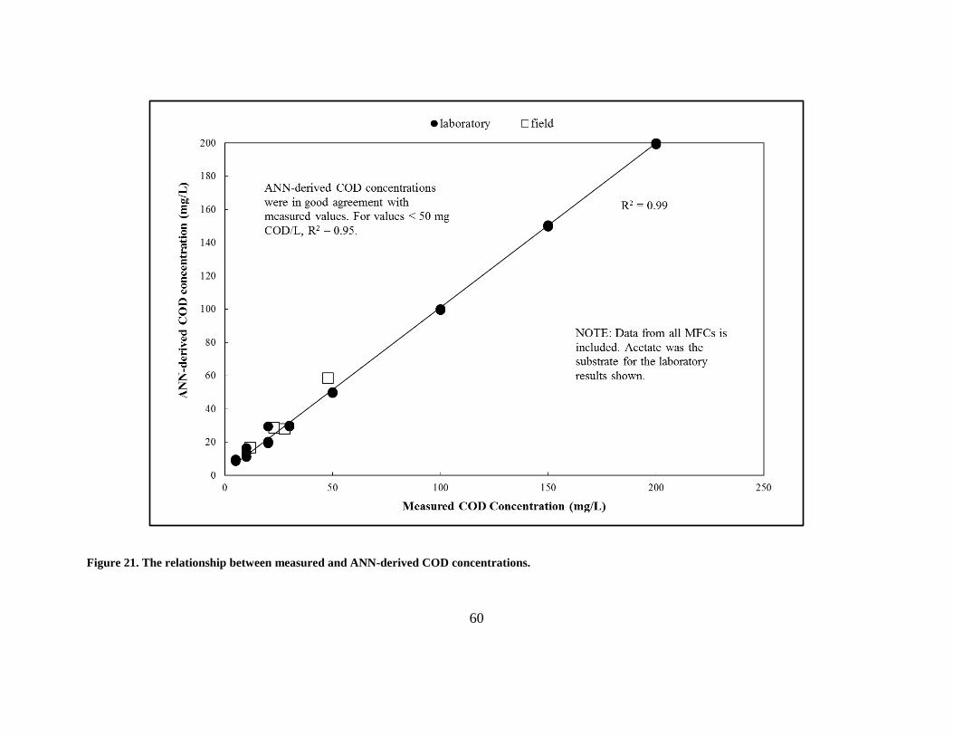
60

Figure 21. The relationship between measured and ANN-derived COD concentrations.

61

I also used the ANN to retrieve two physical properties of the MFCs, the electrode

distance and the anode volume. For these two secondary parameters, I found that one-layer ANN

simulations had low R2 values, but ANNs with two layers had R2 values equal to 1 (Figure 22).

This indicates that retrieving secondary information required a more complicated neural network,

which makes sense because the secondary parameters had a more subtle effect on current

generation. These results have broader implications. In principle, the raw signals produced from

MFCs can be used to determine wide range of operating parameters. For example, the user can

identify parameters related to the MFC device, such as the location or operating condition. The

user may also determine more about the constituents present in a water sample, such as the

presence of particular chemical of concern, the salinity, or the presence of pathogens. The future

efforts will explore the retrieval of these parameters.

62

Figure 22. The relationship between actual and ANN-derived values for secondary parameters.

63

5.2 IDENTIFICATION OF CHEMICALS

5.2.1 Systematic Testing

To identify different chemicals, acetate, butyrate, glucose and corn starch at 50mg as COD/L

were selected as four different substrates to be fed into MFC #1 and MFC #2. Acetate and

butyrate were tested first, followed by glucose and corn starch.

I initially injected acetate into MFCs until the response signals reached a pseudo steady

state, and then I switched to butyrate. For MFC No. 1 in Figure 23(a), acetate generated the

largest values of peak area and height, 1.4mA-hr and 0.08mA respectively. This result was

expected, especially given that the cultures were inoculated with acetate. After I switched to

butyrate, the electrical signals were smaller. For example, for MFC #1 the height of the non-

pseudo steady state butyrate peaks decreased immediately after the substrate transition, followed

by a gradually increasing trend to produce a pseudo steady state PA of 0.07mA-hr and PH of

0.04mA. The pseudo steady state butyrate peaks were smaller than that of acetate. Glucose and

corn starch caused electrical responses that were lower in magnitude than the two acids (as

expected) and very similar to each other. The non-pseudo steady sate peaks of glucose gradually

decreased to a pseudo steady state PH of 0.02mA. The corn starch peaks had similar PH to those

of glucose, however, the signals were structurally different.

64

65

Figure 23. Systematic testing results (a) for MFC #1and (b)for MFC #2.

66

In Figure 23(b) of MFC #2, acetate was again associated with the most prominent

electrical responses, but in this less-responsive sensor, the other peaks were similar in area and

height. The acetate PH and PA were 0.032mA and 0.5mA-hr respectively. The remaining

chemicals induced PH and PA values of approximate 0.002mA and 0.02mA-hr respectively,

significantly smaller than the acetate metrics.

A summary of the average pseudo steady state metrics generated by MFC #1 and MFC

#2 for each of the four substrates was shown in Figure 24. The results for MFC #1 showed that

acetate and butyrate could be easily distinguished with the raw data and without the need for

further neural network processing, but only acetate can be distinguished in MFC #2. These

results demonstrated the limitations associated with trying to identify chemicals using basic

correlations.

67

Figure 24. Systematic testing summary.

68

To further identify the chemicals, a revised ANN was trained and applied where the

specific substrate, as the target of ANN prediction, replaced influent COD into the output layer.

In Figure 25, the ANN successfully discriminated between the peaks of all four substrates for

both MFC #1 and MFC #2, including both the pseudo-steady state and non-pseudo steady state

peaks. It achieved this agreement with one layer of hidden neurons. In this layer, weights, biases,

and the hyperbolic tangent sigmoid transfer function were used to convert the four quantitative

metrics (PA, PH, SR, and AR) into a numerical value on the interval between -1 and 1. These

new values were then propagated to the output layer, which used a linear transfer function to

arrive at a final metric that was associated with one of the four substrates. The key to the ANN

performance was that all four quantitative metrics were used for chemical identification. The

transfer functions propagated information related to the major (i.e. most obvious) response

metrics (PA and PH), as well as the secondary (i.e. more subtle) metrics (AR, SR). This means

that the more subtle differences in the electrochemical signals assist with chemical identification.

For example, glucose and corn starch had PH and PA values that were very similar, but the ANN

accounted for the AR or SR. For example, in MFC #1, the SRs for glucose were1.2-2.7 times

greater than the corn starch SRs and this difference was used to distinguish peaks that are

otherwise similar. Multi-parameter modeling permits accurate chemical discrimination.

69

Figure 25. ANN results in systematic testing.

70

5.2.2 Random Testing

The random testing program demonstrated that the largest signals were associated with acetate,

but these peaks were dynamic (Figure 26). For example in MFC #1, the initial acetate peak

(injection at ~ 50 hours) had a PA and PH of 0.43mA-hr and 0.02mA respectively, but the

acetate peaks observed at 180 and 310 hours had PA and PH values that were significantly (p <

0.01) greater (1.65mA-hr, 0.065mA and 3.47mA-hr, 0.071mA respectively). Interestingly, the

acetate peaks retrieved at later times were also structurally unique, having smaller peak areas.

The electrical signals generated by the other substrates also showed significant temporal

evolution. For example, many of the corn starch and glucose peaks had similar PA and PH to

those generated by butyrate, and a few corn starch peaks are actually larger than the smallest

butyrate peaks. The random testing results for MFC #2 also showed significant temporal

variation (in Figure 27). Clearly, manually interpreting these random signals was difficult, in part

because peaks retrieved at any given time may be influenced by the preceding signal.

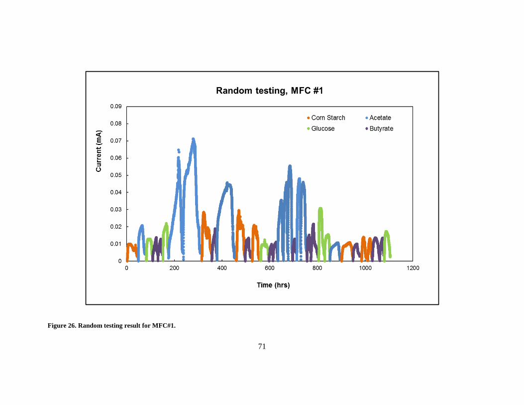
71

Figure 26. Random testing result for MFC#1.

72

Figure 27. Random testing result for MFC #2.

73

ANN modeling of these signals was carried out in two ways. First, I used an ANN that

had three hidden neuron layers (ANN-3), and I trained another that had four hidden layers

(ANN-4). Both ANNs were trained with data taken from systematic testing and some of the data

retrieved from random testing. ANN-3 correctly predicted all acetate peaks, and correctly

predicted the peaks associated with the other chemicals, when they were not preceded by acetate.

When acetate injection preceded that of butyrate, glucose, or corn starch, ANN-3 failed to

correctly predict the post-acetate peak in 26% of the test cases (i.e. 5 of 19 post-acetate test

peaks). This appears to be due lingering effects related to the acetate injection. Specifically, this

could be due to the presence of residual acetate in the anode, or it could be due to an ecological

impact. The acetate “carry-over” effect probably impacted the shape of the post-acetate signals.

Butyrate, glucose, and corn starch did not interfere with the identification of the signal that

followed, likely because these chemicals do not produce peaks that are as prominent as those of

acetate. ANN-4 correctly identified all peaks, including those that appeared after acetate

injection. This showed that a more sophisticated ANN may be needed when different types of

substrates were randomly introduced into the MFC.

74

Figure 28. ANN results in random testing.

75

5.2.3 Factors Related to Chemical Identification

Acetate and butyrate are both non-fermentable substrates, and the present work showed that

these substrates can be distinguished from the fermentable chemicals, glucose and corn starch.

However, I also expected acetate to have a larger PH and PA than butyrate, because the true

microbial growth yield for butyrate (Ybutyrate) is larger than that of acetate (Yacetate) (Metcalf and

Eddy, 2003). This means that the fraction of electrons used for cell synthesis is higher for

butyrate, leaving fewer electrons available for the generation of current. In general, differences in

growth yield should help distinguish between compounds that belong to the same chemical

family.

Electron density is fundamentally related to the biosensor signals, but it is not yet clear

how or when HOMO-LUMO gaps can be used to predict biosensor signals. In principle, it would

be convenient to associate electrical signals with the fundamental chemical properties of a given

constituent, as a type of structure activity relationship useful for biosensing. With this in mind, I

carried out a preliminary investigation to evaluate the possibility that the HOMO-LUMO gap of

a substrate can be used to predict the relative value of two major response metrics, peak area

(PA) and peak height (PH).

The HOMO-LUMO energy gap is a measure of chemical stability (Aihara, 1999).

HOMO stands for highest occupied molecular orbital; LUMO stands for lowest unoccupied

molecular orbital. As the HOMO-LUMO gap increases, more energy is required to excite an

electron to the next orbital, and therefore a larger HOMO-LUMO gap is associated with

increased chemical stability and lower reactivity. I found that the chemicals with the highest

HOMO-LUMO gap had the highest PA and PH (shown in Figure 29). For example, the highest

76

PH and PA are associated with acetate, which has the highest HOMO-LUMO gap of 0.318. The

butyrate PH and PA were 0.04mA and 0.60mA-hr, and the HOMO-LUMO gap was 0.315.

However, these data did not suggest that HOMO-LUMO gap indices were connected to the

relative values of the response metrics.

77

Figure 29. HOMO-LUMO gap data in MFC#1 and MFC#2.

78

5.3 INTEGRATION WITH TSA

Time series analysis (TSA) was also integrated with MFC-based biosensing. To determine how

much data is needed to properly train a time series-model, I studied the relationship between the

training fraction (f) and the average coefficient of determination (R2) is shown in Figure 30. The

f is the fraction of total current data (i.e. data that is on-hand currently) needed to train the TSA

to predict future values. The lowest f value (0.01) resulted in a R2 of 0.93, and I observed a R2 of

0.99 when the f was between 0.05-0.2. When the f exceeded 0.2, I also observed a steep drop in

R2 and I also observed a dramatic increase in the standard deviations. In other words, when I

used values of f greater than 0.2, the quality of the model training was poor on average and it

varied more widely. This is a characteristic of overtraining, which occurs when the model is

fitted to features in the training data set that do not generalize to future time periods.

The TSA regressions also reveal important features. For example, when f = 0.03, the R2 is

0.98, but the regression shows nonlinearity at both high and low current values (Figure 31). The

relatively high R2 value is due to the high density of intermediate current values, but the f value

is not high enough to properly train the network to accurately model the current levels that reside

at either extreme. This shows that a high R2 value is not a sufficient metric for evaluating TSA

model training. When I carried at training at f = 0.2, the R2 value improve slightly, and the

nonlinear regions diminish considerably (Figure 32). These results illustrate why it is best to use

the highest f value that does not cause over-fitting. This critical value was 0.20 in the current

study.

79

Figure 30. The effect of training fraction on coefficient of determination.

80

Figure 31. Training results at f=0.03.

81

Figure 32. Training results at f=0.20.

82

I tested the TSA model on two different time series groups. The first time series was

derived from a MFC exposed to a range of influent COD levels. The properly trained TSA model

predicted the measured values, as expected (Figure 33). The model simulated the shape of the

response peaks and it followed the time-varying magnitude and area associated with the

responses. The model was not as accurate when the measured maximum current levels were

greater than or equal to 0.12mA. This finding is in keeping with what was observed during

training. In other words, the model is less accurate at the highest (and lowest) current levels. The

TSA model also successfully predicted the decreasing current trend that was present in a MFC

was experienced a gradual process failure (Figure 34). The model accurately followed the

decrease from maximum current levels (near 0.06mA) to the lowest current levels (< 0.01).

Further, the model simulated the shape and magnitude of the time-varying peaks. This latter

finding is important because it shows that TSA can be successfully used to predict the need to

maintain or re-inoculate a failing MFC.

83

Figure 33. Temporal current profiles for MFC #1, measurement and modeling.

84

Figure 34. Temporal current profiles for a device requiring maintenance, measurement and modeling.

85

5.4 EFFECT OF BES ADDITION ON DETECTION LIMITS

5.4.1 Effect of BES addition on current production

For less electron consumption by fermenters and methanogens, a lower detection limit can be

generated by a higher peak area, a higher columbic efficiency or a wider dynamic response

range. And 2-bromoethanesulphonate (BES) can inhibit electron consumption by methanogens at

high COD concentrations (Kim et al., 2010; Zhuang et al., 2012). So to further more diminish

detection limits of MFC biosensors, four new cells were utilized lower than 50mg COD/L to test

the effect of BES addition on fermentable and non-fermentable substrates. 50mM BES as

methanogen-specific inhibitor was added into glucose-MFC#7 and 1Mm BES was done into

acetate-MFC#9. And MFC#6 and #8 worked as their control group.

Figure 35 shows the effect of BES on the peak area (PA) for COD concentrations equal

to 50mg/L or less. As expected, the addition of BES caused the peak area to increase when

glucose was added to the MFC. At 50 mg COD/L, the glucose peak areas were 1.31 and

0.71mA-hr with and without BES respectively; the peak area increased by a factor of 1.8.

Significant impacts were observed at 30mg glucose-COD/L (peak areas of 0.89 and 0.11mA-hr

with and without BES respectively), 20mg glucose-COD/L (peak areas of 0.41 and 0.19mA-hr

with and without BES respectively), and 10mg glucose-COD/L (peak areas of 0.37 and 0.05mA-

hr with and without BES respectively). These results make sense because glucose is fermentable,

and BES is known to inhibit methanogens and improve power production in MFCs. BES

86

addition had more subtle impacts on the peak areas generated by acetate addition, and when

20mg acetate-COD/L was injected into the MFCs, the peak areas with and without BES were the

same. These results confirmed that BES addition increased current production in the presence of

fermentable substrates and the impact was observable in the concentration range relevant to an

estuary (i.e. < 50 mg COD/L).

5.4.2 Effect of BES addition on electron balance

In MFCs, electricity is generated through the degradation of organic substrates, so the coulombic

efficiency (CE) was also determined in this study. I found that the columbic efficiencies for these

four MFCs were higher when the COD was lower than 20mg COD/L and the highest CEs were

observed at their lowest COD concentrations (Figure 36).

A dramatic increase of CE was obtained in the presence of BES for glucose at each

corresponding concentration. The difference in CE was 46% at 10mg/l of glucose-COD, 22% at

50mg/l glucose-COD, and the average was 33%. The highest CE in glucose-BES-fed MFC#7

was 71% at 5mg/l COD. The lowest CE was obtained in MFC#6 in the absence of BES (11%) at

30mg/l COD. BES suppresses methanogenesis, which in known to interfere with current

production. CEs for acetate were also improved by the addition of BES but the increase was not

as big as with glucose. The highest CEs of acetate in the presence and absence of BES were 76%

and 40% respectively at the acetate-COD concentration of 5mg/l.

87

Figure 35. The effect of BES addition on peak area for COD < 50 mg/L.

88

Figure 36. The effect of BES addition on coulombic efficiency for COD < 50 mg/L.

89

In MFCs, biomass, residual organic products, and CH4 are possible non-electricity sinks,

and Table 5 summarized the distribution of electron equivalents in all four MFCs at 50mg/l COD

cycles. Except in MFC#6, the residual organic compounds were the largest non-electricity sink:

48.0% for the glucose-BES-MFC#7, 46.0% of the initial COD for the acetate-MFC#8, and

44.0% for the acetate-BES-MFC#9. The unknown portion includes biomass formation and

instrumental loss. In MFC#6, one possible reason for a higher unknown fraction is due to the

growth yield associated with methane-producing cells (Abraham et al., 2005). To detect the

methanogenesis, methane (CH4) was determined in all four MFCs. A low level of CH4 was only

observed in MFC#6 where glucose was fed as fuel and methanogens consumed electrons to

produce methane. No methane was detected in MFC #7 where methanogenesis had been

suppressed by the addition of BES.

Table 5. Electron equivalent balance in four MFCs at COD=50mg/l, expressed as COD (mg).

# of MFC 6 7 8 9

COD (mg)

Fraction (%)

COD (mg)

Fraction (%)

COD (mg)

Fraction (%)

COD (mg)

Fraction (%)

Initial COD 2.000 100.0 2.000 100.0 2.000 100.0 2.000 100.0

Final COD 0.680 34.0 0.960 48.0 0.920 46.0 0.880 44.0

Current 0.212 10.6 0.391 19.6 0.442 22.1 0.549 27.5

Methane 3.68 E-3 0.02 ND -- ND -- ND --

Unknown 1.104 55.38 0.649 32.4 0.638 31.9 0.571 28.5 * Not detected.

90

5.4.3 Integration of ANNs

An increase of peak area with BES addition had been observed in Figure 35 for both glucose and

acetate, but clear linear correlations were lost when COD was lower than 20mg/L, especially for

acetate where similar PAs were present at different COD levels. To better identify these peaks

and expand the direct detection limits, I investigated whether the non-linear complex ANN could

properly interpret the glucose or acetate peaks when the COD concentration is less than 50mg/L.

I re-trained the aforementioned ANN, this time including 15 glucose peaks and 15 acetate peaks

(3 for each COD concentration) in the training data set. The re-trained ANN properly interpreted

the low COD (i.e. < 50mg COD/L) electrical signals for acetate and glucose injections (Figure

37). This means that using the ANN permits proper interpretation of electrical signals at low

COD concentrations when the principle substrate is glucose. So neural network signal processing

expands the detection limit of MFC as biosensor beyond its dynamic range when

methanogenesis suppress cannot work. This result is important, because water quality monitoring

will involve analysis of samples that are known to contain fermentable substrates.

91

Figure 37. ANN correlations for acetate and glucose at COD concentrations less than 50mg/L.

92

6.0 CONCLUSION

This study explored the start-up, operation, and data analysis associated with MFC-based

biosensing. Electrical signals were generated in response to the injection of synthetic water and

field samples, and the results showed a variety of qualitative and quantitative responses that were

generated by single chamber air-cathode MFCs. During laboratory testing, well-organized

normally-distributed responses when the influent COD was 150mg/l or less were observed, while

peaks with two local maxima were observed when the influent COD was 200mg/l. During field

testing, normally-distributed and multi-peak profiles were observed at low COD concentrations

(from 3 to 45mg/l). The peaks with lower COD concentrations produced smaller peak areas

(PAs) and peak heights (PHs). Compared to the results obtained with synthetic water in the

laboratory, field peaks were smaller in size and with longer cycle time. Analysis of all possible

correlations between the influent COD concentration and a variety of quantitative metrics

revealed that the highest coefficient of determination was obtained peak area (PA) was correlated

with the influent COD concentrations, which has not been previously reported. Even higher

coefficients of determination (0.99 for synthetic water and 0.95 for field water) were obtained

with the use of artificial neural network (ANN) model containing just one hidden layer.

It was also established that the MFC electrical signal was dependent on the fed substrates

and ANN processing of MFC data permitted accurate identification of four simple substrates

(acetate, butyrate, glucose and corn starch). Each substrate injection generated four response

93

metrics, namely AR (acceleration rate), SR (subsidence rate), PH (peak height) and PA (peak

area), and these data were used to identify the substrates present in the water samples. As a

result, the non-fermentable substrates, acetate and butyrate, resulted in peak areas (PA) and peak

heights (PH) that were generally larger than those caused by the injection of fermentable

substrates, glucose and corn starch. Acetate generated the most dominant response peaks, PH of

approximate 0.08mA and PA of 1.4mA-hr, respectively. Glucose and corn starch resulted in

electrical signals that were lower than both acids and were very similar in magnitude, about 0.01

mA but structurally different. For the four substrates, it was found that manual discrimination

was only possible for acetate. But when I used the trained ANN, all four substrates were properly

identified using both the sensitive and the less-sensitive biosensor since ANN is multi-parameter

model and allows secondary metrics (such as AR and SR) involved to reflect the structural

differences of various substrates. When different substrates were randomly introduced into MFC

biosensors, the peaks were also correctly identified when an ANN that had four hidden layers of

neurons was employed. The success of ANN-based chemical identification is due to the use of

continuous transfer functions, which propagate information related to all metrics involved.

ANNs should be integrated into water quality monitoring efforts for smart biosensing.

The results also revealed that addition of BES (2-bromoethane sulfonic acid) successfully

inhibited the activity of methanogens in the anode of MFC and increased the magnitude of the

peak area (PA) and columbic efficiency (CE) in laboratory experiments when glucose was the

primary substrate. E.g., at 30 mg-COD/l, the glucose PAs of 0.89 and 0.11mA-hr with and

without BES were observed, increasing by a factor of 8. When glucose was the substrate, a

dramatic increase for CE was also observed in the presence of BES at each COD concentration.

The biggest improvement in CE was 46% at 10mg/l of glucose-COD, and an average increase

94

was 33%. CEs for acetate were also improved by the addition of BES, but not as big as with

glucose. It was revealed that the highest CEs for both acetate and glucose in the presence and

absence of BES were obtained at their lowest COD concentrations. This confirmed that the

methanogenesis suppression was important, especially at very low COD concentrations. It was

also noticed that linear detection limits (the lowest detectable COD concentration) were lost

lower than 20mg/l even in the presence of BES, so a revised ANN was utilized to interpret the

low concentration peaks and the result showed that ANN processing expanded the detection limit

of MFC as biosensor from 20 mg-COD/l to a lower level of 5 mg-COD/l when methanogenesis

suppress cannot work.

Another mathematic model, time series analysis (TSA) with the nonlinear autoregressive

with exogenous input (NARX) method, was also integrated into MFC-based biosensing. It was

found that over-fitting occurred at training fractions greater than 0.2. The properly-trained TSA

model predicted the temporal current trends present in properly functioning MFCs, and in a

device that was gradually failing which predicted the need to maintain or re-inoculation of MFCs

in actual operations.

This work has successfully developed a model that can properly interpret MFC signals, in

spite of the quantitative and structural differences between laboratory and field peaks. It is a

significant accomplishment for water quality monitoring and it establishes a framework with

which MFC-based biosensing can be conducted. This report is the first to integrate artificial

neural network with MFC-based biosensing, the first MFC biosensing effort to propose peak area

as an appropriate response metric and it is also the first to incorporate time series analysis into

MFC-based biosensing. It is now possible to for environmental groups, water utilities, and other

stakeholders to carry out MFC-based biosensing; they simply need to collect the data required to

95

properly train an ANN that can support the monitoring goals. Future research can also exploit

ANNs to determine the concentration of nutrients, electron acceptors, salinity, and other water

quality parameters that are of interest to the water quality community.

96

APPENDIX A

INOCULATION

In this study, ARB activities in the anode chambers were induced by inoculating these MFC

devices with activated sludge, so its induction rates were also investigated and compared.

Inoculation gave rise to a steady electrical signal that is produced by the newly established ARB

community. Each peak generated is response to the injection of both substrate (i.e. acetate) and

activated sludge, and gradually the height and area of the electrical signal increased toward a

nearly constant value.

I observed two distinct inoculation profiles. The first (type I) was observed in the 40ml

MFC#2 and it was a slow, gradually increasing profile (e.g. Figure A1). In this case, each

successive operating cycle gave rise to progressively larger peak area and height values. The

average type I ARB induction rates for MFC#1 and MFC#2 were 0.001mA/day and

0.003mA/day respectively; MFC#2 had a lower internal resistance than MFC#1. The second

(type II) ARB induction profile was observed in the 20ml MFCs and in this case there was an

extensive lag period followed by a relatively fast inoculation rate (e.g. Figure A2). The post-lag

type II ARB induction rates are faster than the more gradual induction rates observed in the type

I profiles. For example, the ARB induction rates for MFC#3 and MFC#5 were 0.0134 and

97

0.0161mA/day respectively. These rates are faster than those associated with the type I

inoculation profiles, and they showed that ARB induction could occur relatively quickly after an

extensive lag period. The 40ml MFCs showed type I induction profiles, whereas the smaller

MFCs showed type II profiles, therefore, the physical dimensions of the MFC biosensor appear

to play a role in causing two distinct ARB induction profiles. This is the first published account

of type II ARB induction in MFC-biosensors.

The type II ARB induction rates documented in the current study are comparable to rates

that have been previously published. For example, the type II ARB induction rates observed in

the current study are in agreement with the rates reported by Peixoto et al. (2011) (average of

0.013mA/day), Gil et al. (0.05mA/day), and Kim et al. (0.05mA/day). Chang et al. (2004)

observed a significantly higher ARB induction rate of approximately 0.20mA/day while

inoculating with glucose and glutamate. None of these previous accounts discussed lag periods.

Future MFC-based biosensor work should document lag periods (when present) and determine

ARB induction rates so that more general trends can be identified.

98

Figure A1. Type I ARB inoculation profile, MFC#2.

99

Figure A2. Type Il ARB inoculation profile, MFC #4.

100

APPENDIX B

DETAILS ON SCMFC ASSEMBLY

Figure B1. Pretreatment for cation exchange membranes (CEMs).

101

Figure B2. Acrylic plates, before and after machining.

102

Figure B3. Drying after application of activated carbon.

Figure B4. Completely assembled SCMFCs, including stabilizing bolts and inlet/outlet ports.

103

APPENDIX C

EXAMPLE MATLAB CODE FOR ANN

C.1 PARAMETERS INVOLVED IN MATLAB CODE FOR ANN

The format for the input matrix is: ['acceleration_rate' deceleration_rate' peak_current' 'current_area'] The acceleration rate is in mA/hr The deceleration rate is in mA/hr The peak current is in mA The current area is in mA-hr The format for the output matrix is: ['inoculation' 'influent_COD' 'anode_volume' 'electrode_distance'] The inoculation is a binary code (1 for yes and 0 for no) The influent_COD is in mg/L The anode volume is in ml The electrode distance is in cm

C.2 OPERATION AND GRAPHING PARTS IN MATLAB CODE FOR ANN

tstart = clock; inputs = [0.008708 -0.001480 0.094727 4.1; 0.010944 -0.002762 0.096474 4.56; 0.016968 -0.002818 0.094373 4.76; 0.038512 -0.008042 0.125 2.8;

104

0.050120 -0.005612 0.129984 2.6; 0.030871 -0.004306 0.124551 3.66; ……

0.000164 -0.000045 0.001767 0.028194; 0.002205 -0.001318 0.004268 0.022404]; targets = [0 200 40 1; 0 200 40 1; 0 200 40 1; 0 150 40 1; 0 150 40 1; 0 150 40 1; …… 0 13.2 20 1; 0 25.3 20 1]; % Preallocate the plotting matrix (PM) PM = zeros (64,10); % the variable of interest is vv (1 for inoculation, 2 for COD, 3 for anode volume, and 4 %for electrode distance) vv = 2; for count = 1:1:10

% Create a Fitting Network hiddenLayerSize = count; net = fitnet(hiddenLayerSize);

% Set up Division of Data for Training, Validation, and Testing net.divideParam.trainRatio = 80/100; net.divideParam.valRatio = 10/100; net.divideParam.testRatio = 10/100;

% Train the Network [net,tr] = train(net,inputs,targets);

% Test the Network outputs = net(inputs); errors = gsubtract(outputs,targets); performance = perform(net,targets,outputs);

% View the Network %view(net)

plotperf(tr)

Outputs = net(inputs); %trOut = Outputs(tr.trainInd); %vOut = Outputs(tr.valInd); %tsOut = Outputs(tr.testInd); %trTarg = Outputs(tr.trainInd); %vTarg = targets(tr.valInd); %tsTarg = targets(tr.testInd); %plotregression(trTarg,trOut,'Train',vTarg,vOut,'Validation',tsTarg,tsOut,'Testing');

PM(:,count) = Outputs(:,vv);

end

105

figure(1) %plot(targets(:,vv),PM(:,1),'ro',targets(:,vv),PM(:,2),'r-')

plot(targets(:,vv),PM(:,1),'ko',targets(:,vv),PM(:,2),'r-',targets(:,vv),PM(:,3),'--m+',targ ets(:,vv),PM(:,4),'bv',targets(:,vv),PM(:,5),'kx') title('Targets vs. Outputs') xlabel('Targets') ylabel('Outputs') legend('1 layer','2 layers','3 layers','4 layers','5 layers')

%AXIS([50 200 50 200]) figure(2) %plot(targets(:,vv),PM(:,1),'ro',targets(:,vv),PM(:,2),'r-')

plot(targets(:,vv),PM(:,6),'ko',targets(:,vv),PM(:,7),'r-',targets(:,vv),PM(:,8),'--m+',targets(:,vv),PM(:,9),'bv',targets(:,vv),PM(:,10),'kx') title('Targets vs. Outputs') xlabel('Targets') ylabel('Outputs') legend('6 layers','7 layers','8 layers','9 layers','10 layers')

%AXIS([50 200 50 200]) tstop = clock; runtime = etime(tstop,tstart); disp('length of run in seconds:') disp(runtime)

106

APPENDIX D

EXAMPLE MATLAB CODE FOR TSA

D.1 PARAMETERS INVOLVED IN MATLAB CODE FOR TSA

Parameter “a” is the time point and parameter “b” is the relative current. Load INPUTS and OUTPUTS INPUT defines many 2-element input vectors (column vectors) OUTPUT defines the associated 1-element targets (column vectors) Figure(3) is for a linear model for prediction. Figure(4) is for investigating residuals. Figure(5) is for comparing the linear model and the original free response.

D.2 OPERATION AND GRAPHING PARTS IN MATLAB CODE FOR TSA

a=[0.482883333 0.549552778 … 46.8179575]; b=[1.48936E-05 0.002461702

107

… 0.010580851]; for i = 3:1391,

INPUT(1,i-2) = b(i-1); INPUT(2,i-2) = b(i-2); OUTPUT(i-2) = b(i);

end %OUTPUT(1389) = OUTPUT(1389); % Let's make a linear model (and recover coefficients c1 and c2): parameters = INPUT'\OUTPUT'; predictions = INPUT' * parameters; figure(3) plot(predictions) % Let’s investigate residuals residuals = predictions - OUTPUT'; figure(4) plot(residuals) % Note change of vertical scale. % Let's compare the linear model and the original free response point(1) = 1.48936E-05; point(2) = 1.48936E-05; for i = 1:1391

response(i) = parameters(1)*point(1) + parameters(2)*point(2); point(2) = point(1); point(1) = response(i);

end figure(5) plot(1:1391,response,'r-',1:1391,b,'b--') legend('model','data');

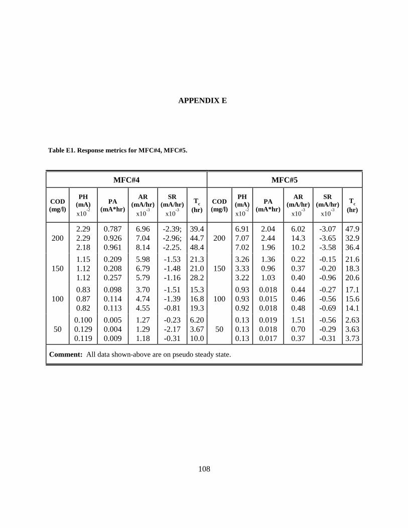
108

APPENDIX E

Table E1. Response metrics for MFC#4, MFC#5.

MFC#4 MFC#5

COD (mg/l)

PH (mA) x10

-2

PA (mA*hr)

AR (mA/hr)

x10-3

SR (mA/hr)

x10-3

Tc (hr)

COD (mg/l)

PH (mA) x10

-2

PA (mA*hr)

AR (mA/hr)

x10-3

SR (mA/hr)

x10-3

Tc (hr)

200 2.29 2.29 2.18

0.787 0.926 0.961

6.96 7.04 8.14

-2.39; -2.96; -2.25.

39.4 44.7 48.4

200 6.91 7.07 7.02

2.04 2.44 1.96

6.02 14.3 10.2

-3.07 -3.65 -3.58

47.9 32.9 36.4

150 1.15 1.12 1.12

0.209 0.208 0.257

5.98 6.79 5.79

-1.53 -1.48 -1.16

21.3 21.0 28.2

150 3.26 3.33 3.22

1.36 0.96 1.03

0.22 0.37 0.40

-0.15 -0.20 -0.96

21.6 18.3 20.6

100 0.83 0.87 0.82

0.098 0.114 0.113

3.70 4.74 4.55

-1.51 -1.39 -0.81

15.3 16.8 19.3

100 0.93 0.93 0.92

0.018 0.015 0.018

0.44 0.46 0.48

-0.27 -0.56 -0.69

17.1 15.6 14.1

50 0.100 0.129 0.119

0.005 0.004 0.009

1.27 1.29 1.18

-0.23 -2.17 -0.31

6.20 3.67 10.0

50 0.13 0.13 0.13

0.019 0.018 0.017

1.51 0.70 0.37

-0.56 -0.29 -0.31

2.63 3.63 3.73

Comment: All data shown-above are on pseudo steady state.

109

BIBLIOGRAPHY

Abraham, E.N., Mary, R., Manju, S. and Lovley, D.R. (2005). Growth of Geobacter sulfurreducens under nutrient-limiting conditions in continuous culture. Environmental Microbiology 7(5), 641-648.

Aihara, J. (1999). Reduced HOMO-LUMO gap as an index of kinetic stability for polycyclic aromatic hydrocarbons. Journal of Physical Chemistry A 103(37), 7487-7495.

APHA (1992). Standard Methods for the Examination of Water and Wastewater (18th edition). American Public Health Association, American Water Works Association, Water Pollution Control Federation, Washington, D.C..

Aulenta, F., Catervi, A., Majone, M., Panero, S., Reale, P. and Rossetti, S. (2007). Electron transfer from a solid-state electrode assisted by methyl viologen sustains efficient microbial reductive dechlorination of TCE. Environmental Science & Technology 41(7), 2554-2559.

Ayenew, T. and Legesse, D. (2007). The changing face of the Ethiopian rift lakes and their environs: call of the time. Lakes and reservoirs: Research & Management 12(3), 149-165.

Bachmann, T.T. and Schmid, R.D. (1999). A disposable multielectrode biosensor for rapid simultaneous detection of the insecticides paraoxon and carbofuran at high resolution. Analytica Chimica Acta 401, 95-103.

Beliaev, A.S. and Saffarini, D.A. (1998). Shewanella putrefaciens mtrB encodes an outer membrane protein required for Fe(III) and Mn(IV) reduction. Journal of Bacteriology 180(23), 6292-6297.

Bergel, A., Feron, D. and Mollica, A. (2005). Catalysis of oxygen reduction in PEM fuel cell by seawater biofilm. Electrochemistry Communications 7(9), 900-904.

110

Black, J. G. (2002). Microbiology: principles and explorations (5th edition). Wiley, New York, NY.

Bond, D.R., Holmes, D.E., Tender, L.M. and Lovley, D.R. (2002). Electrode-reducing microorganisms that harvest energy from marine sediments. Science 295(5554), 483-485.

Bond, D.R. and Lovley, D.R. (2003). Electricity production by Geobacter suljiurreducens attached to electrodes. Applied and Environmental Microbiology 69(3), 1548-1555.

Borole, A.P., Mielenz, J.R., Vishnivetskaya, T.A. and Hamilton, C.Y. (2009). Controlling accumulation of fermentation inhibitors in biorefinery recycle water using microbial fuel cells. Biotechnology for Biofuels 2, 7.

Brillinger, D.R. (1975). Time series: Data analysis and theory. New York: Holt, Rinehart.&Winston.

Chae, K.J., Choi, M.J., Kim, K.Y., Ajayi, F.F., Park, W., Kim, C.W. and Kim, I.S. (2010). Methanogenesis control by employing various environmental stress conditions in two-chambered microbial fuel cells. Bioresource Technology 101(14), 5350-5357.

Chang, I.S., Jang, J.K., Gil, G.C., Kim, M., Kim, H.J., Cho, B.W. and Kim, B.H. (2004). Continuous determination of biochemical oxygen demand using microbial fuel cell type biosensor. Biosensors & Bioelectronics 19(6), 607-613.

Chee, G.J., Nomura, Y., Ikebukuro, K. and Karube, I. (2000). Optical fiber biosensor for the determination of low biochemical oxygen demand. Biosensors & Bioelectronics 15(7-8), 371-376.

Chee, G.J., Nomura, Y., Ikebukuro, K. and Karube, I. (2005). Development of photocatalytic biosensor for the evaluation of biochemical oxygen demand. Biosensors & Bioelectronics 21(1), 67-73.

Chiu, P.C. and Lee, M. (2001). 2-Bromoethanesulfonate affects bacteria in a trichloroethene-dechlorinating culture. Applied and Environmental Microbiology 67(5), 2371-2374.

Choi, S. and Chae, J. (2012). Optimal biofilm formation and power generation in a micro-sized microbial fuel cell (MFC). Sensors and Actuators A, In Press.

111

Cressie, N. and Holan, S.H. (2011). Special issue on time series in the environmental sciences. Journal of Time Series Analysis 32(4), 337-338.

Cohen, B. (1931). The bacterial culture as an electrical half-cell. Journal of Bacteriology 21, 18-19.

Dobbin, P.S., Powell, A.K., McEwan, A.G. and Richardson, D.J. (1995). The influence of chelating-agents upon the dissimilatory reduction of Fe(III) by Shewwzella putrefuciens. Biometals 8(2), 163-173.

Fan, Y., Hu, H. and Liu, H. (2007). Enhanced coulombic efficiency and power density of air-cathode microbial fuel cells with an improved cell configuration. Journal of Power Sources 171(2), 348-354.

Ghumman, A. R. (2011). Assessment of water quality of Rawal Lake by long-time monitoring. Environmental Monitoring and Assessment 180(1-4), 115-126.

Gregory, K.B., Vidic, R.D. and David, A.D. (2011). Water management challenges associated with the production of shale gas by hydraulic fracturing. Elements 7(3), 181-186.

Gomes, L., Troiani, E.P. and Nozaki, J. (2011). Analysis of the environmental impact on a stream: Is only tannery to blame? Environmental Monitoring and Assessment 173(1-4), 489-498.

Gorby, Y.A. and Beveridge, T.J. (2005). Composition, reactivity, and regulation of extracellular metal-reducing structures (nanowires) produced by dissimilatory metal reducing bacteria. Warrenton, VA.

Gupta, I., Dhage, S. and Kumar, R. (2009). Study of variations in water quality of Mumbai Coast through multivariate analysis technique. Indian Journal of Marine Sciences 38(2), 170-177.

Hatch, J.L. and Finneran, K.T. (2008). Influence of reduced electron shuttling compounds on biological H2 production in the fermentative pure culture Clostridium beijerinckii. Current Microbiology 56, 268-273.

Howell, T. (1993). Non-linear Time Series: A Dynamical System Approach. Oxford.

112

Juahir, H., Zain, S.M., Yusoff, M.K., Hanidza, T.T.I., Armi, A.S.M., Toriman, M.E. and Mokhtar, M. (2011). Spatial water quality assessment of Langat River Basin (Malaysia) using environmetric techniques. Environmental Monitoring and Assessment 173(1-4), 625-641.

Kang, K.H., Jang, J.K., Pham, T.H., Moon, H., Chang, I.S. and Kim, B.H. (2003). A microbial fuel cell with improved cathode reaction as a low biochemical oxygen demand. Biotechnology Letters 25(16), 1357-1361.

Kazi, T.G., Arain, M.B., Jamali, M.K., Jalbani, N., Afridi, H.I. and Sarfraz, R.A. (2009). Assessment of water quality of polluted lake using multivariate statistical techniques: A case study. Ecotoxicology and Environmental Safety 72(20), 301-309.

Keery, J., Andrew, B., Nigel, C. and Smith, J.W.N. (2007). Temporal and spatial variability of groundwater–surface water fluxes: Development and application of an analytical method using temperature time series. Journal of Hydrology 336(1-2), 1-16.

Khadka, R.B. and Khanal, A.B. (2008). Environmental Management Plan (EMP) for Melamchi water supply project, Nepal. Environmental Monitoring and Assessment 146(1-3), 225-234.

Kiely, P.D., Rader, G., Regan, J.M. and Logan, B.E. (2011). Long-term cathode performance and the microbial communities that develop in microbial fuel cells fed different fermentation endproducts. Bioresource Technology 102(1), 361-366.

Kim, B.H., Chang, I.S., Gil, G.C., Park, H.S. and Kim, H.J. (2003). Novel BOD sensor using mediator-less microbial fuel cell. Biotechnology Letters 25(7), 541-545.

Kim, B.H., Park, D.H., Shin, P.K., Chang, I.S. and Kim, H.J. (1999a). Mediator-less biofuel cell. U.S. Patent 5976719.

Kim, B.H., Park, H.S., Kim, H.J., Kim, G.T., Chang, I.S., Lee, J., Phung, N.T. (2004b). Enrichment of microbial community generating electricity using a fuel-cell-type electrochemical cell. Applied Microbiology and Biotechnology 63(6), 672–681.

Kim, D.K., Jeong, K.S., McKay, R.I.B., Chon, T.S. and Joo, G.J. (2012). Machine learning for predictive management: short and long term prediction of phytoplankton biomass using genetic algorithm based recurrent neural networks. International Journal of Environmental Research 6(1), 95-108.

113

Kim, H.J., Hyun, M.S., Chang, I.S. and Kim, B.H. (1999b). A microbial fuel cell type lactate biosensor using a metal-reducing bacterium, Shewanella putrefaciens. Journal of Microbiology and Biotechnology 9(3), 365-367.

Kim, J.R., Jung, S.H., Regan, J.M. and Logan, B.E. (2007). Electricity generation and microbial community analysis of alcohol powered microbial fuel cells. Bioresource Technology 98(13), 2568-2577.

Kim, M.N. and Kwon, H.S. (1999). Biochemical oxygen demand sensor using Serratia marcescens LSY 4. Biosensors & Bioelectronics 14(1), 1-7.

Kim, M.S. and Lee, Y.J. (2010). Optimization of culture conditions and electricity generation using Geobacter sulfurreducens in a dual-chambered microbial fuel-cell. International Journal of Hydrogen Energy 35(23), 3028-3034.

Kim, I.S., Hwang, M.H., Jang, N.J., Hyun, S.H. and Lee, S.T. (2004a). Effect of low pH on the activity of hydrogen utilizing methanogen in bio-hydrogen process. International Journal of Hydrogen Energy 29(11), 1133-1140.

Kim, I.S., Chae, K.J., Choi, M.J., Kim, K.Y., Ajayi, F.F., Park, W. and Kim, C.W. (2010). Methanogenesis control by employing various environmental stress conditions in two-chambered microbial fuel cells. Bioresource Technology 101(14), 5350-5357.

Kralisch, S., Fink, M., Flügel, W.A. and Beckstein, C. (2003). A neural network approach for the optimisation of watershed management. Environmental Modelling & Software 18(8-9), 815-823.

Kumlanghan, A., Liu, J., Thavarungkul, P., Kanatharana, P. and Mattiasson, B. (2007). Microbial fuel cell based biosensor for fast analysis of biodegradable organic matter. Biosensors & Bioelectronics 22(12), 2939-2944.

Lanthier, M., Gregory, K.B., Lovley D.R. (2008). Growth with high planktonic biomass in Shewanella oneidensis fuel cells. FEMS Microbiology Letters 278(1), 29-35.

Larminie, J. and Dicks, A. (2000). Fuel cell systems explained. John Wiley & Sons.

Lee, J.H., Mitchell, R.J., Kim, B.C., Cullen, D.C. and Gu, M.B. (2005). A cell array biosensor for environmental toxicity analysis. Biosensors & Bioelectronics 21(3), 500-507.

114

Lemberg, R. and Barrett, J. (1973). Cytochromes. London, New York.

Li, C.L. and Fang, H.H.P. (2007). Fermentative hydrogen production from wastewater and solid wastes by mixed cultures. Critical Reviews in Environmental Science and Technology 37(1), 1-39.

Li, W.W., Sheng, G.P., Liu, X.W., Cai, P.J., Sun, M., Xiao, X., Wang, Y.K., Tong, Z.H., Dong, F. and Yu, H.Q. (2011). Impact of a static magnetic field on the electricity production of Shewanella-inoculated microbial fuel cells. Biosensors & Bioelectronics 26(10), 3987-3992.

Liao, V.H.C., Chien M.T, Tseng, Y.Y. and Ou K.L (2006). Assessment of heavy metal bioavailability in contaminated sediments and soils using green fluorescent protein-based bacterial biosensors. Environmental Pollution 142(1), 17-23.

Liu, H. and Logan, B.E. (2004). Electricity generation using an air-cathode single chamber microbial fuel cell in the presence and absence of a proton exchange membrane. Environmental Science & Technology 38(14), 4040-4046.

Liu, J. and Mattiasson, B. (2002). Microbial BOD sensors for wastewater analysis. Water Research 36(15), 3786-3802.

Logan, B.E., Cheng, S., Watson, V. and Estadt, G. (2007). Graphite fiber brush anodes for increased power production in air-cathode microbial fuel cells. Environmental Science & Technology 41(9), 3341-3346.

Logan, B.E. (2004). Extracting hydrogen and electricity from renewable resources. Environmental Science & Technology 38(9), 160A-167A.

Logan, B.E. (2007). Microbial Fuel Cells. John Wiley & Sons Publishers, Hoboken, N.J..

Lorenzo, M.D., Curtis, T.P., Head, I.M. and Scott, K. (2009). A single-chamber microbial fuel cell as a biosensor for wastewaters. Water Research 43(13), 3145-3154.

Lovley, D.R. (2008). Extracellular electron transfer: wires, capacitors, iron lungs, and more. Geobiology 6, 225-231.

115

Lower, S.K., Hochella, M.F. and Beveridge, T.J. (2001). Bacterial recognition of mineral surfaces: nanoscale interactions between Shewanella and α-FeOOH. Science 292(5520), 1360-1363.

Lu, C.J., Lee, T.S. and Chiu, C.C. (2009). Financial time series forecasting using independent component analysis and support vector regression. Decision Support Systems 47(2), 115-125.

Maier, H.R., Morgan, N. and Chow, C.W.K. (2004). Use of artificial neural networks for predicting optimal alum doses and treated water quality parameters. Environmental Modelling & Software 19(5), 485-494.

Marrazza, G., Chianella, I. and Mascini, M. (1999). Disposable DNA electrochemical biosensors for environmental monitoring. Analytica Chimica Acta 387, 297-307.

Marquardt, D. (1963). An algorithm for least-squares estimation of nonlinear parameters. SIAM Journal on Applied Mathematics 11(2), 431-441.

Marsili, E., Baron, D.B., Shikhare, I.D., Coursolle, D., Gralnick, J.A. and Bond, D.R. (2008). Shewanella secretes flavins that mediate extracellular electron transfer. Proceedings of the National Academy of Sciences 105(10), 3968-3973.

MathWorks, Inc. (2012). MATLAB® Data Analysis. Natick, MA.

Metcalf and Eddy (2003). Wastewater Engineering: Treatment and Reuse. McGraw-Hill Publishers, New York, NY.

Min, B., Kim, J.R., Oh, S., Regan, J.M. and Logan, B.E. (2005). Electricity generation from swine wastewater using microbial fuel cells. Water Research 39(20), 4961-4968.

Mohan, S.V., Saravanan, R., Raghavulu, S.V., Mohanakrishna, G. and Sarma, P.N. (2008). Bioelectricity production from wastewater treatment in dual chambered microbial fuel cell (MFC) using selectively enriched mixed microflora: Effect of catholyte. Bioresource Technology 99(3), 596-603.

Moon, H., Chang, I.S., Kang, K.H., Jang, J.K. and Kim, B.H. (2004). Improving the dynamic response of a mediator-less microbial fuel cell as a biochemical oxygen demand (BOD) sensor. Biotechnology Letters 26(22), 1717-1721.

116

Mustafa, G. and Catbas, F.N. (2011). Structural health monitoring and damage assessment using a novel time series analysis methodology with sensor clustering. Journal of Sound and Vibration 330(6), 1196-1210.

Myers, J.M. and Myers, C.R. (2001). Role for outer membrane cytochromes OmcA and OmcB of Shewanella putrefaciens MR-1 in reduction of manganese dioxide. Applied and Environmental Microbiology 67(1), 260-269.

Oh, S.E. and Logan, B.E. (2005). Hydrogen and electricity production from a food processing wastewater using fermentation and microbial fuel cell technologies. Water Research 39(19), 4673-4682.

Oh, S.E., Min, B. and Logan, B.E. (2004). Cathode performance as a factor in electricity generation in microbial fuel cells. Environmental Science & Technology 38(8), 4900-4904.

Parellada, J., Narvaez, A., Lopez, M.A., Dominguez, E., Fernandez, J.J., Pavlov, V. and Katakis, I. (1998). Amperometric immunosensors and enzyme electrodes for environmental applications. Analitica Chimica Acta 362, 47-57.

Park, D.H., Laivenieks, M., Guettler, M.V., Jain, M.K. and Zeikus, J.G. (1999). Microbial utilization of electrically reduced neutral red as the sole electron donor for growth and metabolite production. Applied and Environmental Microbiology 65(7), 2912-2917.

Park, D.H. and Zeikus, J.G. (2002). Impact of electrode composition on electricity generation in a single-copartment fuel cell using Shewanella putrefucians. Applied Microbiology and Biotechnology 59(1), 58-61.

Park, D.H. and Zeikus, J.G. (2003). Improved fuel cell and electrode designs for producing electricity from microbial degradation. Biotechnology and Bioengineering 81(3), 348-355.

Patricio, P. (2012). Combined model for PM10 forecasting in a large city. Atmospheric Environment 60, 271-276.

Paul, S. and Diana, S. (2006). Dictionary of Microbiology & Molecular Biology (3rd edition). Chichester, West Sussex ; Hoboken, NJ : Wiley.

117

Peixoto, L., Min, B., Martins, G., Brito, A.G., Kroff, P., Parpot, P., Angelidaki, I. and Nogueira, R. (2011). In situ microbial fuel cell-based biosensor for organic carbon. Bioelectrochemistry 81, 99-103.

Ponomareva, O., Arlyapov, V., Alferov, V. and Reshetilov, A. (2011). Microbial biosensors for detection of biological oxygen demand. Applied Biochemistry and Microbiology 47(1), 1-11.

Potter, M.C. (1911). Electrical effects accompanying the decomposition of organic compounds. Proceeding of the Royal Society B 84(571), 260-276.

Rabaey, K., Boon, N., Hofte, M. and Verstraete, W. (2005). Microbial phenazine production enhances electron transfer in biofuel cells. Environmental Science & Technology 39(9), 3401-3408.

Rabaey, K. and Verstraete, W. (2005). Microbial fuel cells: novel biotechnology for energy generation. TRENDS in Biotechnology 23(6), 291-298.

Reguera, G., McCarthy, K.D., Mehta, T., Nicoll, J.S., Tuominen, M.T. and Lovley, D.R. (2005). Extracellular electron transfer via microbial nanowires. Nature 435(7045), 1098-1101.

Reguera, G., Nevin, K.P., Nicoll, J.S., Covalla, S.F., Woodard, T.L., and Lovley, D.R. (2006). Biofilm and nanowire production leads to increased current in Geobacter sulfurreducens fuel cells. Applied and Environmental Microbiology 72(11), 7345-7348.

Richter, H., Nevin, K.P., Jia, H., Lowy, D.A., Lovley, D.R., and Tender, L.M. (2009). Cyclic voltammetry of biofilms of wild type and mutant Geobacter sulfurreducens on fuel cell anodes indicates possible roles of OmcB, OmcZ, type IV pili, and protons in extracellular electron transfer. Energy & Environmental Science 2(5), 506-516.

Riedel, K., Renneberg, R., Kuhn, M. and Scheller, F. (1988). A fast estimation of biochemical oxygen demand using microbial sensors. Applied and Environmental Microbiology 28, 316-318.

Rittmann, B.E., Parameswaran, P., Torres, C.I., Lee, H.S. and Rosa K.B. (2009). Syntrophic interactions among anode respiring bacteria (ARB) and Non-ARB in a biofilm anode: electron balances. Biotechnology and Bioengineering 103(3), 513-523.

118

Rosenbaum, M., Aulenta, F., Villano, M. and Angenent, L.T. (2011). Cathodes as electron donors for microbial metabolism: Which extracellular electron transfer mechanisms are involved? Bioresource Technology 102(1), 324-333.

Sara R.M., Maria J.L.A. and Damià B. (2006). Biosensors as useful tools for environmental analysis. Analytical and Bioanalytical Chemistry 386(4), 1025-1041.

Schwartz, I.B., Billings, L., Pancrazio, J.J. and Schnur, J.M. (2001). Methods for short time series analysis of cell-based biosensor data. Biosensors & Bioelectronics 16(7-8), 503-512.

Schalkoff, R. (1997). Artificial neural networks. McGraw-Hill Publishers, New York, NY.

Shumway, R.H. (1988). Applied statistical time series analysis. Englewood Cliffs, NJ: Prentice Hall.

Singh, K.P., Malik, A., Singh, V.K., Mohan, D. and Sinha, S. (2005). Chemometric analysis of groundwater quality data of alluvial aquifer of Gangetic Plain, North India. Analytica Chimica Acta 550(1-2), 82-91.

Snyman, J.A. (2005). Practical mathematical optimization: An introduction to basic optimization theory and classical and new gradient-based algorithms. Springer Publishing.

Stavros, I.D., Nikolaos, A.L., Vasso, T., Michael, V., Sifis, M. and Spiros, F. (2010). Tracking brain dynamics via time-dependent network analysis. Journal of Neuroscience Methods 193, 145-155.

Steinbusch, K.J., Hamelers, H.V., Schaap, J.D., Kampman, C. and Buisman, C.J. (2010). Bioelectrochemical ethanol production through mediated acetate reduction by mixed cultures. Environmental Science & Technology 44(1), 513-517.

Su, L., Jia, W., Hou, C. and Lei, Y. (2011). Microbial biosensors: a review. Biosensors & Bioelectronics 26(5), 1788-1799.

Tan, T.C. and Wu, C. (1999). BOD sensors using multi-species living or thermally killed cells of a BODSEED microbial culture. Sensors and Actuators B 54(3), 252-260.

119

Tateo, Y. (1992). The biochemistry of bacterial cytochromes. Tokyo: Japan Scientific Societies Press, Berlin, New York: Springer-Verlag.

Tortora, G.J., Funke B.R., Case C.L. (2007). Microbiology: an introduction (9th edition). San Francisco: Pearson Benjamin Cummings.

Tschmelak, J, Proll, G. and Gauglitz, G. (2004). Ultra-sensitive fully automated immunoassay for the detection of propanil in aqueous samples - steps of progress towards a sub-nanogram per liter detection. Analytical and Bioanalytical Chemistry 379, 1004-1012.

Venkataraman, A., Rosenbaum, M., Arends, J.B.A., Halitsche, R. and Angenent, L.T. (2010). Quorum sensing regulates electric current generation of Pseudomonas aeruginosa PA14 in bioelectrochemical systems. Electrochemistry Communications 12(3), 459-462.

Wei, J., Liang, P., Cao, X., and Huang, X. (2010). A new insight into potential regulation on growth and power generation of Geobacter sulfurreducens in microbial fuel cells based on energy viewpoint. Environmental Science & Technology 44(8), 3187-3191.

Wen, Y. and Zeng, B. (1999). A simple nonlinear filter for economic time series analysis. Economics Letters 64, 151-160.

Yerel, S. (2010). Water quality assessment of Porsuk River, Turkey. E-Journal of Chemistry 7(2), 593-599.

You, S., Zhao, Q., Zhang, J., Jiang, J., Wan, C., Dua, M. and Zhao, S. (2007). A graphite-granule membrane-less tubular air-cathode microbial fuel cell for power generation under continuously operational conditions. Journal of Power Sources 173, 172-177.

You, S., Zhao, Q., Zhang, J., Jiang, J. and Zhao, S. (2006). A microbial fuel cell using permanganate as the cathodic electron acceptor. Journal of Power Sources 162, 1409-1415.

Zhang, E., Xu, W., Diao, G. and Shuang, C. (2006). Electricity generation from acetate and glucose by sedimentary bacterium attached to electrode in microbial-anode fuel cells. Journal of Power Sources 161, 820-825.

Zhuang, L., Chen, Q., Zhou, S., Yuan, Y. and Yuan, H. (2012). Methanogenesis control using 2-Bromoethanesulfonate for enhanced power recovery from sewage sludge in air-cathode microbial fuel cells. International Journal of Electrochemical Science 7, 6512-6523.

120

Zinder, S.H. and Koch, M. (1984). Non-acetoclastic methanogenesis from acetate: acetate oxidation by thermophilic syntrophic coculture. Archives of Microbiology 138(3), 263-272.

Zuo, Y., Cheng, S., Call, D. and Logan, B.E. (2007). Tubular membrane cathodes for scalable power generation in microbial fuel cells. Environmental Science & Technology 41(9), 3347-3353.