Semi-transitive graphs

Semi-Transitive Graphs

Steve WilsonDEPARTMENT OF MATHEMATICS AND STATISTICS

NORTHERN ARIZONA UNIVERSITY FLAGSTAFF

ARIZONA 86011-5717

E-mail: [email protected]

Received March 15, 2000; Revised April 9, 2003

DOI 10.1002/jgt.10152

Abstract: In this paper, we first consider graphs allowing symmetrygroups which act transitively on edges but not on darts (directed edges).We see that there are two ways in which this can happen and we introducethe terms bi-transitive and semi-transitive to describe them. We examinethe elementary implications of each condition and consider families ofexamples; primary among these are the semi-transitive spider-graphsPS(k,N;r ) and MPS(k,N;r ). We show how a product operation can be usedto produce larger graphs of each type from smaller ones. We introduce thealternet of a directed graph. This links the two conditions, for each alternetof a semi-transitive graph (if it has more than one) is a bi-transitive graph.We show how the alternets can be used to understand the structure ofa semi-transitive graph, and that the action of the group on the set ofalternets can be an interesting structure in its own right. We use alternetsto define the attachment number of the graph, and the important specialcases of tightly attached and loosely attached graphs. In the case of tightlyattached graphs, we show an addressing scheme to describe the graphwith coordinates. Finally, we use the addressing scheme to complete theclassification of tightly attached semi-transitive graphs of degree 4 begunby Marusic and Praeger. This classification shows that nearly all suchgraphs are spider-graphs. � 2003 Wiley Periodicals, Inc. J Graph Theory 45: 1–27, 2004

Keywords: graph symmetry; graph automorphism; alternet; semi-transitive graph

� 2003 Wiley Periodicals, Inc.

1

1. PRELIMINARIES

All graphs considered in this paper are connected, and have no loops or parallel

edges. We think of an edge of the graph � as an unordered pair fu; vg of vertices.

If fu; vg is an edge of �, we think of the ordered pair ðu; vÞ as a directed edge

from u to v. We call ðu; vÞ a dart (or arc or directed edge) of �. If � is a graph, a

symmetry (or automorphism) of � is a permutation of its vertices which preserves

edges. Autð�Þ is the collection of all symmetries of �, and it is a group under

composition. If two vertices (or two edges) are in the same orbit under Autð�Þ,we call the two vertices (or edges) similar.

Consider a graph � such that Autð�Þ contains a subgroup G which is transitive

on the edges of � but not on its darts. Let d be any one dart of �. Then the orbit of

d under G consists of one dart from each edge. We can think of this orbit of darts

as a directed graph �. We call � an orientation of �.

Consider a vertex v and consider the edges of � which meet v. There are two

possibilities:

I: v is a source or a sink (that is, it has only out-directed edges or only in-

directed edges) or

II: v meets at least one in-directed edge and at least one out-directed edge.

Because all vertices at the heads of darts of � must be in the same orbit, and

similarly for tails, we see that if case II holds at v then every vertex has both in-

and out-directed edges; therefore, if case I holds at v, every vertex must be a

source or a sink.

2. BI-TRANSITIVE GRAPHS

Consider case I briefly. Every vertex is a source or a sink and every edge leads

from one to the other. So the graph is bi-partite (i.e., two-colorable) and every

edge leads from, say, a white vertex to a black vertex. We say that � is bi-

transitive and that � is a bi-transitive orientation for �. Then all of the white

vertices are in one orbit and so must all have the same degree d; all black vertices

are in the other orbit and have the same degree e. If W and B are the numbers of

vertices of each color, then the easy count gives dW ¼ E ¼ eB. Of course if

W 6¼ B, the graph cannot be vertex transitive.

Looking at it the other way, we will call a graph � bi-transitive provided that it

is bipartite and that Autþð�Þ, the group of color-preserving automorphisms of �,

is transitive on edges. We say � is strictly bi-transitive provided that it is bi-

transitive and Autþð�Þ ¼ Autð�Þ.

2.1. Examples

1. The graph KM;N is bi-transitive for all M, N, and strictly bi-transitive unless

M ¼ N.

2 JOURNAL OF GRAPH THEORY

2. Let X be the set f1; 2; 3; 4; . . . ;Ng. The graph PðN; a; bÞ, defined for

integers 0 < a < b < N, has two kinds of vertices: the black vertices

correspond to subsets of X of size b, the whites to subsets of X of size a. The

set A of size a is connected to a set B of size b exactly when A � B.

PðN; a; bÞ is bi-transitive for all a; b;N, and strictly bi-transitive unless

a þ b ¼ N.

3. A slight generalization, TðN; a; b; cÞ, has vertices corresponding to sets of

size a and b, with two sets connected when their intersection has size c.

In the first two of these examples, the graph is dart-transitive whenever B ¼ W

and d ¼ e. A graph is called regular provided that all of its vertices have the same

degree. In this case, regular means that d ¼ e, and B ¼ W . Many examples of

strictly bi-transitive graphs in which B ¼ W are unworthy, i.e., they have the

property that same two distinct vertices have exactly the same set of neighbors.

We will discuss later a construction that gives an example which is regular,

strictly bi-transitive and worthy. A graph which is regular and strictly bi-transitive

is called semi-symmetric, and some very fruitful research is being done in the case

of semi-symmetric graphs in which d ¼ e ¼ 3.

3. SEMI-TRANSITIVE GRAPHS AND THEIR ORIENTATIONS

Now we examine case II with some care.

If every vertex of � has both in- and out-edges, then again because all vertices

at the heads of darts must be in the same orbit, the group must be transitive on

vertices. Let d be the number of heads and e the number of tails per vertex. Then

the easy count yields dV ¼ E ¼ eV , from which we get d ¼ e, so that every

vertex of � has degree 2d.

We will call such a graph semi-transitive, and the directed graph � a (semi-

transitive) orientation for �. If � is an orientation for �, then so is the directed

graph ��, in which every arrow in � has been reversed. Looking at it the other

way, we call a graph � semi-transitive provided that (1) it is the underlying graph

of a directed graph � such that Autð�Þ is transitive on edges and on vertices, or

equivalently, (2) Autð�Þ has a subgroup G which acts transitively on edges and

on vertices, but not on darts. If Autð�Þ ¼ Autð�Þ, we say � is strictly semi-

transitive, or 1/2-transitive. A semi-transitive graph is dart-transitive if there is a

symmetry which reverses an edge, and otherwise, it is 1/2-transitive. Equivalently

it is dart-transitive when Autð�ÞnAutð�Þ is non-empty.

The notion of a 1/2-transitive graph was the beginning of this topic, with a

simple result (that 1/2-transitive graphs have even degree) by Tutte in 1966 [13].

In 1970, Bouwer [3] proved that there are infinitely many 1/2-transitive graphs,

and that they exist with all possible degrees. In 1981, Holt [6], gave an example

of one of degree 4 with 27 vertices. In 1991, Alspach et al. [1] showed this to

be the smallest such graph. In the late 1990s Marusic, Waller, and Nedela made

progress on 1/2-transitive graphs of degree 4 [8,9,12], while Du and Xu examined

SEMI-TRANSITIVE GRAPHS 3

those having group actions which are primitive on the vertices [4,5]. Semi-

transitive and 1/2-transitive graphs are of interest in their own right, and their

study is also motivated by the study of group actions having non-self-paired

orbitals, as in [10].

3.1. Examples

Let us first examine some families of semi-transitive graphs:.

The Power-Spidergraph, PS(k,N; r). This, named by my student Leah

Berman in Ref. [2] and called Xðr; k;NÞ in [8], is the natural generalization

of Holt’s original example. The numbers must satisfy k � 2;N � 3; rk � �1

(mod N). There are kN vertices, which we think of as being arranged in k

concentric rings and N spokes, as in Figure 1. The vertices in one ring are joined

only to vertices in the ring before and after. By regarding the set of vertices as

Zk � ZN , we can use coordinates to show the edges explicitly: each ði; jÞ is joined

to ði þ 1; j � riÞ. See Figure 1.

FIGURE 1. � ¼PS (3, 7; 2).


In fact, if we let PS½k;N; r� be the directed graph �, with each edge leading

from ði; jÞ to ði þ 1; j � riÞ, we can show that � is a semi-transitive orientation for

the undirected graph PSðk;N; rÞ.Consider the functions:

ði; jÞ� ¼ ði; j þ 1Þði; jÞ� ¼ ði;�jÞði; jÞ� ¼ ði þ 1; rjÞ.

We can see that these are symmetries of �. For example, we apply � to the

directed edge

ði; jÞ ! ði þ 1; j þ riÞ:

First, the image of the initial vertex is ði; jÞ� ¼ ði þ 1; rjÞ; second, the image of

the terminal vertex is ði þ 1; j þ riÞ� ¼ ði þ 2; rðj þ riÞÞ ¼ ði þ 2; rj þ riþ1Þ, and

finally,

ði þ 1; rjÞ ! ði þ 2; rj þ riþ1Þ

is an edge of the graph and a directed edge of the directed graph. Thus � is a

symmetry of the graph and of the digraph.

From � and �, we see that all vertices in one ring are similar, and all edges in

the webbing directed from one ring to the next are similar. Then � sends every

vertex lying in one ring to the next ring in, and so these symmetries act semi-

transitively on the graph, and so PSðk;N; rÞ is semi-transitive.

It is not hard to see that if r2 ¼ �1 mod N then the graph is dart-transitive.

It may be dart-transitive in other cases. The smallest such is � ¼ PSð3; 7; 2Þ,shown in Figure 1.

Holt’s original example of a (1/2)-transitive graph is PSð3; 9; 2Þ. For Holt’s

graph, both Autð�Þ and Autð�Þ have order 54. In the graph � ¼ PSð3; 7; 2Þ,contrastingly, Autð�Þ has order 42ð¼ EÞ, while Autð�Þ has order 336, so this

graph is not 1/2-transitive; i.e., it is dart-transitive. The graph � has many

interesting properties and we will meet it again several times later in this paper.

Marusic [8] classifies all dart-transitive power-spidergraphs for odd values of N.

Mutant Power-Spidergraphs: MPS (k,N; r). This is a slight modification of

PSðk;N; rÞ. Again with k;N, greater than 2; rk � �1 mod N, and N even, we

regard the vertices as Zk � ZN . We use coordinates to show the edges explicitly:

each ði; jÞ is joined to ði þ 1; j � riÞ except when i ¼ k � 1; then ðk � 1; jÞ is

joined to ð0; j þ N=2 � rk�1Þ. This describes a directed graph � ¼ MPS½k;N; r�and the following symmetries apply:

ði; jÞ� ¼ ði; j þ 1Þði; jÞ� ¼ ði;�jÞði; jÞ� ¼ ði þ 1; rjÞ if i < k � 1

ðk � 1; jÞ� ¼ ð0; rj þ N=2Þ

�


We can see that these are symmetries of �, and that they act semi-transitively on

the graph, so MPSðk;N; rÞ is semi-transitive. The question of dart-transitivity for

these graphs is still open.

Notice that if k and N are both even (and so r is odd), then PS½k;N; r� has two

components: one in which edges join (even, even) to (odd, odd) to (even even)

and one in which (even odd) is joined to (odd, even) to (even, odd). Similarly, if k

and M are both even or both odd, then MPS½k; 2M; r� has two components. In

each case, we reassign the name PS½k;N; r� or MPS½k; 2M; r� to the connected

component containing (0,0).

With these conventions in place, we see that a number of isomorphisms

between spidergraphs hold; these are listed in the Appendix. By using facts A–F

from this list, we can show that every directed spidergraph is isomorphic to one in

which the number of vertices is kN=2, rather than kN. This is the form referred to

in the final theorem of this paper.

Cayley graphs. These are well-known in general. If S is any subset of a

group G not containing the identity of G, we can define the directed graph

� ¼ Cay½G; S� whose vertices are the elements of G; its edges are of the form

g ! xg where x is an element of S. The undirected graph of � ¼ Cay½G; S� is the

underlying graph of Cay½G; S�. Any Cayley digraph or graph is vertex-transitive,

because for each h in G, the function g ! gh is a symmetry of both � and �.

Thus G, as a subgroup of Autð�Þ, acts transitively on the vertices of �.

Suppose now that H is a subgroup of AutðGÞ, and that b is an element of G

such that the orbit S of b under H is ‘‘closed against inverses,’’ i.e., that if x is in

S; x�1 is not in S. Then H acts as a group of symmetries of � and �. H acts

transitively on the edges emanating from the identity vertex in �. Together with

G (in a semi-direct product) these symmetries act edge-and vertex-transitively on

�, showing that the Cayley graph � is semi-transitive.

If H is a subgroup of a subgroup K of AutðGÞ such that the orbit of b under K is

S [ S�1, (i.e., fx 2 Gjx 2 S or, x�1 2 SgÞ, or, equivalently, if there is f in AutðGÞsuch that f normalizes H and f ðbÞ ¼ b�1, then the graph is dart-transitive. It may

be dart-transitive in other circumstances, however. The graph �, shown in

Figure 1, may also be regarded as a Cayley graph for the non-abelian group of

order 21 with two generators of order 3. This graph is dart-transitive, although the

subgroup K suggested above does not exist.

The directed graph shown in Figure 2, above, is the Cayley digraph for A4 with

generating set S ¼ fð2 3 4Þ; ð1 3 4Þ; ð1 2 4Þ; ð1 2 3Þg.

Circulant graphs. These are a special case of Cayley graphs but worth

separate attention. Let S be a non-empty subset of the non-zero numbers mod N.

The circulant digraph CN ½S� has ZN as its vertex set, with directed edges i ! i þ s

for each i in ZN ; s in S. The circulant graph CNðSÞ is its underlying graph. If S is a

subgroup of UN , the multiplicative group of units mod N, and does not contain

�1, then CNðSÞ is semi-transitive; of course, it may be semi-transitive in many

other circumstances. The directed graph shown below is C13½1; 3; 9�. It is a semi-

transitive orientation of C13ð1; 3; 4Þ.


Wreaths and depleted wreaths. For integers k � 3;N � 2, the wreath graph

Wðk;NÞ has kN vertices arranged in a circle of k bunches of N vertices each.

Every vertex in one bunch is joined by edges to every vertex in the bunch

immediately before and after it in circular order. If we direct the edges from

bunch i to bunch i þ 1 mod k, this is clearly a semi-transitive orientation of the

graph.

The depleted wreath graph, DWðk;NÞ is formed from Wðk;NÞ by removing

the edges of n disjoint k-cycles from the graph. DWðk;NÞ is semi-transitive.

Figure 4 below shows Wð5; 3Þ and DWð5; 3Þ:We can label the vertices with ordered pairs from Zk � ZN , and say that

vertex ði; jÞ is connected all vertices ði þ 1; hÞ in Wðk;NÞ, and ði; jÞ is connected

to all ði þ 1; hÞ with h 6¼ j in DWðk; nÞ. The orientations are given by ði; jÞ !ði þ 1; hÞ.

FIGURE 2. Cayley digraph for A 4.


Wðk;NÞ is always a circulant graph; Wðk;NÞ ¼ CkNðSÞ where S ¼ fx 2ZkN jx � �1ðmod kÞg. DWðk;NÞ is circulant if k and N are relatively prime and

not otherwise.

Medial graphs. If M is an orientable rotary map, its medial graph is formed

on the same surface by creating one new vertex at the midpoint of each edge, and

then joining two of these if they appear consecutively around some face. The

graph is called MGðMÞ. If we orient the new edges so that each one points

FIGURE 3. C13[1, 3, 9]

FIGURE 4. W (5, 3) and DW (5, 3).


counter-clockwise about the face of M in which it appears (and hence clockwise

about its vertex), the result is an orientation of MGðMÞ: a rotation around a face

(or a vertex) of M preserves the map and so MGðMÞ, and also preserves the

orientation of the surface and so the orientations of the edges. Thus the group

AutþðMÞ, of orientation-preserving symmetries of M, acts semi-transitively on

MGðMÞ. So every MG of an orientable rotary map is semi-transitive.

Figure 5, below, shows the cube (in thin lines) and its medial graph, directed,

in bold lines.

If M is reflexible, then a reflection is an orientation-reversing symmetry of

MG, and so the graph is dart-transitive. If the map is directly self-dual, i.e. if there

is an orientation-preserving homeomorphism of the surface onto itself which

sends the map to its dual, then also, MG is dart-transitive. It may be dart-transitive

in other circumstances as well; for example M ¼ f3; 6g2;1 is a non-self-dual

chiral (non-reflexible) rotary map, but its medial graph is the graph � which we

know to be dart-transitive.

Products. If �1 and �2 are graphs, the product �1 � �2 is a graph whose

vertices are ordered pairs of vertices from the factors, with ða; bÞ connected to

FIGURE 5. The cube and its medial graph.


ðc; dÞ if fa; cg is an edge in �1 and fb; dg is an edge in �2. If each factor is

connected, then the product is connected unless both factors are bipartite, in

which case the product has two components, one in which ðW ;WÞ vertices are

connected to ðB;BÞ vertices and one in which ðB;WÞ’s are connected to ðW ;BÞ’s.

For example, (Figs. 6 and 7):

It is clear that if �i is in Autð�iÞ; i ¼ 1; 2, then �, defined by ða; bÞ� ¼ ða�1; b�2Þ, is in Autð�1 � �2Þ. From this, we derive the following list of

results:

1. If �1 and �2 are vertex-transitive then �1 � �2 is vertex-transitive.

2. If �1 and �2 are dart-transitive then �1 � �2 is dart-transitive.

3. If �1 is dart-transitive and �2 is semi-transitive then �1 � �2 is semi-

transitive.

4. If �1 and �2 are bitransitive then each component of �1 � �2 is bitransitive.

Fact 4 enables us to construct bitransitive graphs which are worthy and which

might be strictly bitransitive. �1 ¼ Pð5; 4; 2Þ has 5 black vertices of degree 6 and

10 white vertices of degree 3. �2 ¼ Pð5; 2; 1Þ has 10 black vertices of degree 2

and 5 white vertices of degree 4. So one component of � ¼ �1 � �2 has 50 black

vertices of degree 12 and 50 white vertices of degree 12. So � is bitransitive,

regular and worthy. It is, I claim, strictly bitransitive.

To see this most easily, note that in �1 and �2, any two vertices of the same

color have at least one common neighbor, except for black vertices in �2 (such as

{1,2} and {3,4}). Then in the product �, every pair of white vertices will have a

common neighbor but some pairs of black vertices will not. Therefore, no

FIGURE 6. k1, 2 and k1, 3.

FIGURE 7. k1, 2� k1, 3.


symmetry can interchange white and black vertices, and so � is strictly bi-

transitive.

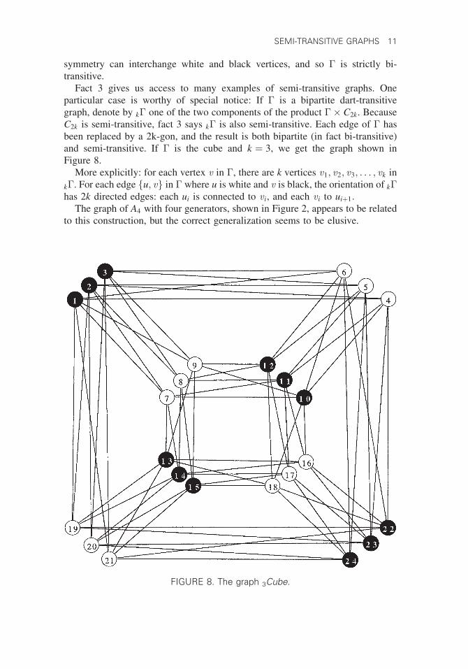
Fact 3 gives us access to many examples of semi-transitive graphs. One

particular case is worthy of special notice: If � is a bipartite dart-transitive

graph, denote by k� one of the two components of the product �� C2k. Because

C2k is semi-transitive, fact 3 says k� is also semi-transitive. Each edge of � has

been replaced by a 2k-gon, and the result is both bipartite (in fact bi-transitive)

and semi-transitive. If � is the cube and k ¼ 3, we get the graph shown in

Figure 8.

More explicitly: for each vertex v in �, there are k vertices v1; v2; v3; . . . ; vk in

k�. For each edge fu; vg in � where u is white and v is black, the orientation of k�has 2k directed edges: each ui is connected to vi, and each vi to uiþ1:

The graph of A4 with four generators, shown in Figure 2, appears to be related

to this construction, but the correct generalization seems to be elusive.

FIGURE 8. The graph 3Cube.


4. ALTERNETS

Suppose that � is an orientation for a semi-transitive graph �. Declare two

directed edges to be ‘‘related’’ if they have the same initial vertex or if they have

the same terminal vertex. Consider the equivalence relation generated by

‘‘related.’’ In the case d ¼ 2, an equivalence class for this relation is a cycle; this

is called an alternating cycle in Marusic [8]. In the general case, we will use the

term alternet for the sub-graph consisting of an equivalence class of directed

edges.

Autð�Þ acts on the alternets; i.e., the alternets are blocks of imprimitivity for

the action of Autð�Þ on the edges of �. If the alternets are A1;A2;A3; . . . ; let Hi

be the set of all vertices at the heads of arrows in Ai and let Ti be the set of all

vertices at the tails of arrows in Ai. The Hi’s, the head-sets, partition the vertex set

as do the Ti’s, the tail-sets.

If A ¼ Hi \ Tj is non-empty, we will call the set A an attachment set.

All attachment sets have the same size. If A ¼ Hi ¼ Tj, we call � tightly

attached. If A is a singleton, we call � loosely attached. The size of A must

divide the size of any Hi, and we call this the attachment number of �.

These definitions naturally extend those of Marusic [8] and Marusic and

Praeger [11].

Let’s examine alternets in several of our examples.

(1) Spidergraphs. Here the alternets lie in the webbing between two con-

secutive rings. If N is odd, a tail-set consists of the entire ring of vertices ði; jÞ for a

fixed i and the corresponding head-set is the ring of all ði þ 1; jÞ. If N is even (and

so r must be odd), the webbing between ring i and i þ 1 has two components, one

with tail-set consisting of all ði; 2jÞ’s and head-set all ði þ 1; 2j þ 1Þ’s, the other

vice versa. Each of these components is an alternet. Each head-set is also a tail-set

and so the graph is tightly attached. The attachment number is N if N is odd, N=2

if N is even.

(2) In MGðMÞ, each alternet is a cycle running along a Petrie path in M. Here

the tail-sets are (usually) distinct from the head-sets.

(3) In Cay½G; S�, vertex g has edges pointing to s1g; s2g; . . . ; where si’s are the

elements of S. The vertices at the tails of edges pointing toward these vertices are

all of the form s�1j sig. Vertices at the tails of edges pointing to vertices these point

to are vertices of the form s�1m sks�1

j sig, and so on. The tail-set for this alternet will

be the coset Kg of the group K generated by all elements of the form s�1j si. The

head-set is the coset LSg of the group L generated by all elements of the form

sjs�1i . Of course, in an abelian group, K and L will be identical. The attachment

number in any case is the size of K \ L.

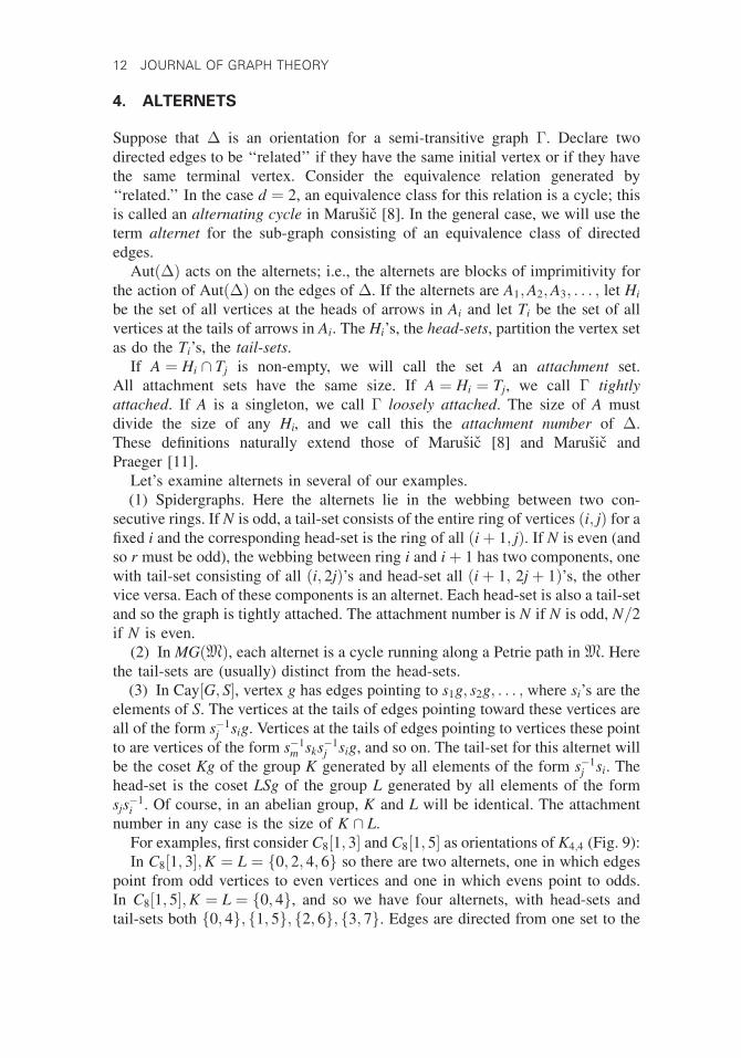
For examples, first consider C8½1; 3� and C8½1; 5� as orientations of K4;4 (Fig. 9):

In C8½1; 3�;K ¼ L ¼ f0; 2; 4; 6g so there are two alternets, one in which edges

point from odd vertices to even vertices and one in which evens point to odds.

In C8½1; 5�;K ¼ L ¼ f0; 4g, and so we have four alternets, with head-sets and

tail-sets both f0; 4g; f1; 5g; f2; 6g; f3; 7g. Edges are directed from one set to the


next. Thus, these two digraphs are non-isomorphic semi-transitive orientations

for K4;4.

In C13½1; 3; 9� (Fig. 3), K ¼ L ¼ Z13, so there is only one alternet. This shows

that in the general case, it is possible to have just one alternet. Marusic shows in

Ref. [8] that if vertices have degree 4, this is not possible. In graphs in which the

group action is primitive (see [4,5]) on the vertices, there can be only one alternet.

If there is more than one alternet, then each alternet is a bipartite graph, the

tail-set forming one color class, the head-set the other. Moreover, Autð�Þ,restricted to one alternet, acts transitively on the edges of the alternet. Thus each

alternet is bi-transitive.

(4) In k�, the alternet having white vertex ui in a tail-set is a copy of �consisting of all vertices with subscript i; if the black vertex vi is in a tail-set, the

alternet consists of all black vertices having subscript i and whites having i þ 1,

again a copy of �. This shows that any bipartite dart-transitive graph can be the

alternet of a semi-transitive graph. Whether this is true for a strictly bi-transitive

graph is not yet known. In fact, I do not know of any semi-transitive graph whose

alternets are strictly bi-transitive (and so semi-symmetric).

5. SEMI-SIMPLIFICATION

We label the alternets 1; 2; 3; . . . ; etc. in any order. Then we can assign labels to

vertices by giving the label hi; ji to a vertex which is in the head-set of i and the

tail-set of j. Thus any edge in alternet j points from a vertex with label hi; ji to a

FIGURE 9. C8[1, 3] and C8[1, 5].


vertex with label hj; ki for some i; k depending on the edge. The diagrams in

Figures 10 and 11 show this labelling in the medial graphs of the tetrahedron and

the cube:

In MGðTÞ, Figure 10, notice that there are only three vertex labels:

h1; 2i; h2; 3i; h3; 1i. This is similar to the case PSðk;N; rÞ where the only vertex

labels are hi; i þ 1i. Whenever two or more vertices share the same label, we can

form a simplified directed graph by using the vertex labels as vertices, and

making an edge from ha; bi to hc; di exactly when b ¼ c. This new graph is

automatically semi-transitive and loosely attached, and we will call it the semi-

simplification of the original.

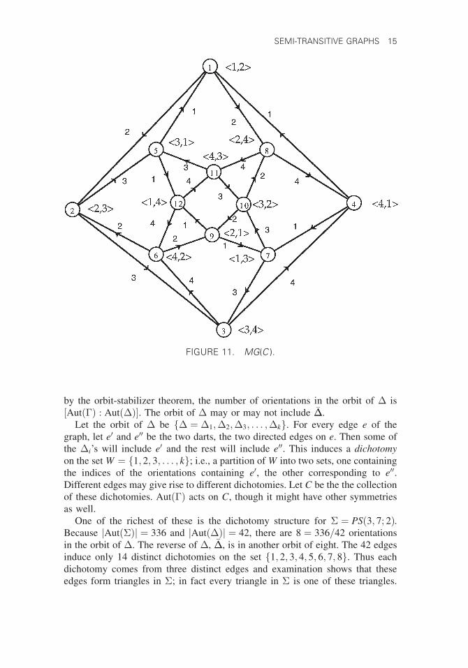
Now consider the medial graph of the cube, MGðCÞ, shown in Figure 11:

Here, contrastingly, no two vertices have the same label, and so if we try to

make a simplified labelling as above, we get the same graph back; it is already

loosely attached, and so its semi-simplification is itself. An interesting direc-

tion for research, I think, is this question: Given a loosely attached graph, which

semi-transitive graphs are there which simplify to it? Even in the case of the

cycles Ck, this is unsolved. A second question: can we classify loosely attached

graphs?

6. ORBITS OF ORIENTATIONS AND DICHOTOMIES

Let � be a semi-transitive graph and let � be an orientation for �. If � is not

strictly semi-transitive then it has orientations other than � and its reversal ��.

Then Autð�Þ acts on the class of orientations. In the context of this action, we

may regard Autð�Þ to be the stabilizer of the object � in the group Autð�Þ. Then

FIGURE 10. MG(T ).


by the orbit-stabilizer theorem, the number of orientations in the orbit of � is

½Autð�Þ : Autð�Þ�. The orbit of � may or may not include ��.

Let the orbit of � be f� ¼ �1;�2;�3; . . . ;�kg. For every edge e of the

graph, let e0 and e00 be the two darts, the two directed edges on e. Then some of

the �i’s will include e0 and the rest will include e00. This induces a dichotomy

on the set W ¼ f1; 2; 3; . . . ; kg; i.e., a partition of W into two sets, one containing

the indices of the orientations containing e0, the other corresponding to e00.Different edges may give rise to different dichotomies. Let C be the the collection

of these dichotomies. Autð�Þ acts on C, though it might have other symmetries

as well.

One of the richest of these is the dichotomy structure for � ¼ PSð3; 7; 2Þ.Because jAutð�Þj ¼ 336 and jAutð�Þj ¼ 42, there are 8 ¼ 336=42 orientations

in the orbit of �. The reverse of �, ��, is in another orbit of eight. The 42 edges

induce only 14 distinct dichotomies on the set f1; 2; 3; 4; 5; 6; 7; 8g. Thus each

dichotomy comes from three distinct edges and examination shows that these

edges form triangles in �; in fact every triangle in � is one of these triangles.

FIGURE 11. MG(C ).


The dichotomy structure, called the Capuzzi Dichotomies after the student who

studied these first, is listed below:

1 : 1 2 3 4 --- 5 6 7 8

2 : 2 3 4 5 --- 6 7 8 1

3 : 3 4 5 6 --- 7 8 1 2

4 : 4 5 6 7 --- 8 1 2 3

5 : 2 3 6 8 --- 1 4 5 7

6 : 3 4 7 1 --- 2 5 6 8

7 : 4 5 8 2 --- 3 6 7 1

8 : 5 6 1 3 --- 4 7 8 2

9 : 6 7 2 4 --- 5 8 1 3

10 : 7 8 3 5 --- 6 1 2 4

11 : 8 1 4 6 --- 2 3 5 7

12 : 1 2 5 7 --- 3 4 6 8

13 : 1 4 5 8 --- 2 3 6 7

14 : 2 5 6 1 --- 3 4 7 8

We can speak of two numbers (orientations) as being on the same side of, or on

opposite sides of, a given dichotomy. In dichotomy 14, for example, 1 and 2 are

on the same side while 1 and 3 are on opposite sides. In �, every pair of numbers

lie on the same side of exactly 6 dichotomies while any three lie on the same side

of exactly 2.

If we compare two dichotomies x and y, there are two possibilities: (I) we

might find that the four numbers on one side of x lie two on one side and

two on the other in y, or (II) it might be that the four on one side of x have three

on one side of y and one on the other. For each x there are 4 y’s that overlap

x as in case II. If we make a graph with 14 vertices corresponding to dicho-

tomies and two connected if the overlap is 3-1, we get the graph shown in

Figure 12.

The surprising thing about this graph is that it is bipartite, that the dicho-

tomies come in two essentially different kinds. The two classes are f1; 3; 5;7; 9; 11; 14g and f2; 4; 6; 8; 10; 12; 13g. If we form the ‘‘bipartite complement’’

of this graph (i.e., remove existing edges and then connect every vertex to all

vertices of the other color to which it was not previously connected), we get

the Heawood graph, i.e., the incidence graph for Fano’s plane. That there

should be a connection of some sort between � and the Heawood graph is not

in itself so surprising, as � is the line graph of Heawood. We examine these

connections:


First, the above says we can label the points and lines of the Fano plane as

shown in Figure 13, so that a point lies on a line exactly when the two corres-

ponding labels belong to dichotomies that overlap in the 2-2 pattern.

The structure has a second connection to Fano’s plane. Specifically, choose

any of the numbers from 1 to 8 and call it x; and choose one of the two

color classes of dichotomies. For each of those seven dichotomies, write down the

three other numbers on the same side as x. This list of seven 3-tuples is the Fano

plane.

FIGURE 12. Overlap graph.

FIGURE 13. The Fano plane with labels.


For example, consider orientation 1 and the class f2; 4; 6; 8; 10; 12; 13g. The

sides of these that contain 1 are: f1; 6; 7; 8g; f1; 2; 3; 8g; f1; 3; 4; 7g; f1; 3; 5; 6g;f1; 2; 4; 6g; f1; 2; 5; 7g; f1; 4; 5; 8g. Remove ‘‘1’’ from each of these and we have

the presentation of Fano’s plane shown in Figure 14.

This means that Fano’s plane is symmetrically embedded in the Capuzzi

Dichotomies in 16 interlocking ways. Will this structure generalize in any

interesting way? Perhaps the next graph to look at in this respect is PSð6; 5; 2Þwith 60 edges. There are 12 orientations in one orbit for this graph, and the

dichotomy structure on these 12 objects should be interesting.

7. TIGHTLY-ATTACHED GRAPHS

In this section, we discuss the structure of tightly attached semi-transitive graphs

and construct a sort of cordinate system for such a graph.

Let us suppose that � is semi-transitive, that � is an orientation of �, that � is

tightly-attached, and that � has at least two alternets. Let L0; L1;L2; . . . ;Lk�1 be

the ‘‘levels,’’ i.e., the head- and tail-sets, so that every edge of � leads from a

vertex in some Li to some vertex in Liþ1 mod k. We restrict our attention to the

case in which no two distinct elements of Li have exactly the same set of

neighbors in Liþ1 and vice-versa. In other words, we assume each alternet is

worthy.

FIGURE 14. One side of one color class.


Let T be the group of all symmetries of � which fix L0 (and hence all levels),

and let � be any one symmetry which sends each Li to Liþ1. Assign the labels

ð0; 1Þ; ð0; 2Þ; ð0; 3Þ; . . . ð0;NÞ to the vertices of L0 at random. Assign labels to

L1; L2; . . . :; Lk�1 by:

ði; jÞ� ¼ ði þ 1; jÞ:

Then we must have:

ðk � 1; jÞ� ¼ ð0; j�Þ

for some permutation � in SN . It follows that ð0; jÞ��1 ¼ ðk � 1; j��1Þ.We call this labeling process and its result an addressing scheme for �.

For each � in T , define �0; �1; �2; . . . ; �k�1 by ði; jÞ� ¼ ði; j�iÞ. Thus each �i is in

SN and represents the permutation on the labels in level i induced by the action of

� . We abbreviate this by saying that � ¼ ð�0; �1; �2; ; �k�1Þ. Let Ti be the set of all

�i such that � is in T . Then each Ti is a subgroup of SN . Notice that, as a

consequence of the worthy assumption, a vertex in Li is determined by its

neighbors in Liþ1 and vice versa. Then each �i determines � uniquely. So the

function � : �0 ! � ! �1 is an isomorphism of T0 onto T1.

Now suppose � is any element of T and consider the action of ��1:

If i < k � 1 : ði; jÞ��1 ¼ ði þ 1; jÞ��1 ¼ ði þ 1; j�iþ1Þ��1 ¼ ði; j�iþ1Þ

If i ¼ k � 1 : ðk � 1; jÞ��1 ¼ ð0; j�Þ��1 ¼ ð0; j��0Þ��1

¼ ðk � 1; j��0��1Þ:

We learn several things about the addressing scheme from this computation:

1. to use the notation above, if � ¼ ð�0; �1; �2; . . . ; �k�1Þ, then we have that

��1 ¼ ð�1; �2; . . . ; �k�1; ��0��1Þ.

Since every permutation that occurs at level 1 also appears at level 0, we can

conclude that:

2. T0 ¼ T1 ¼ T2 ¼ � � � ¼ Tk�2 ¼ Tk�1. Call this group T.

Then:

3. � is an automorphism of T.4. every element of T looks like ð�0; �ð�0Þ; �2ð�0Þ; �3ð�0Þ; . . . ; �k�1ð�0ÞÞ for

some �0 in T.

Now �k must be in T . Examining the labelling process, we see that:

5. �k ¼ ð�; �; �; . . . ; �Þ and this is in T , so � is in T.6. from the fourth and fifth fact, we see that �ð�Þ ¼ �.


7. from the fact that ð�1; �2; . . . ; �k�1; ��0��1Þ is in T , we have that

�ð�k�1Þ ¼ ��0��1.

Then ��0��1 ¼ �ð�k�1Þ ¼ �ð�k�1ð�0ÞÞ ¼ �kð�0Þ, and this says that �k is an

inner automorphism of T; it is, in fact, conjugation by �.

These facts together give us the structure of tightly-attached semi-transitive

graphs. Every such graph has a symmetry group satisfying these requirements,

and conversely, every group satisfying these requirements acts as the group of

such a graph.

8. THE DEGREE 4 CASE

We wish to use the addressing scheme developed above to prove a result which

sharpens and simplifies a theorem of Marusic and Praeger in [11]. We want to

claim in the theorem that nearly all tightly-attached graphs of degree 4 are

spidergraphs, plain or mutant. There are some special cases to note:

(1) If the graph has exactly two alternets, Marusic and Praeger in [11] show

that the graph must be C2Nð1; aÞ for some a 6� �1 such that a2 � �1

(mod 2N). We note that this graph can be described as PSð2; 2N; aÞ.(2) If the head-sets have size 2, then every vertex in one is connected to every

vertex in the next. This describes the wreath graph Wðk; 2Þ. If k is even

then Wðk; 2Þ is isomorphic to (one component of) PSðk; 4; 1Þ. If k is odd,

it is not a spider-graph of any kind.

(3) Recall that the notation PS½k;N; r� or MPS½k;N; r� refers to one component

of the digraph constructed and so often has kN=2 vertices.

With these in mind, we can state and prove the following:

Theorem 8.1. Suppose that � is a tightly attached semi-transitive graph of

degree 4 having k alternets and head-sets of size N. If N ¼ 2 and k is odd, � must

be Wðk; 2Þ. Otherwise it is PS(k, N; r) or PS(k, 2N; r) or MPS(k, 2N; r) for some r.

Proof. We first note that Marusic [8] shows that in the degree 4 case, there

cannot be exactly one alternet. From comments above, we see that the theorem is

true if the number k of alternets is 2. We also see that if N ¼ 2, we know the

graph is a wreath graph, which is a spider-graph when k is even. Then we are left

to consider the case k � 3;N � 3. This implies that each alternet is worthy and so

the addressing scheme applies.

Since every vertex has degree 4, the alternets must be cycles. The length of

each alternet cycle must be 2N; there are k of them. Then T , the group that

preserves alternets, must be the dihedral group DN . The proof divides into cases

based on the parity of N. We begin each case by establishing some notation for

dihedral groups.


8.1. The Even Case

If N is even, N ¼ 2M, denote the vertices of a regular N-gon by 0; 1; 2; 3; 4; . . . ;N � 1;N ¼ 0 and the reflections by x0; y1; x2; y3; x4; . . . ; yN�1; xN, where x2i is

the reflection with axis through i and i þ M, and y2iþ1 has the axis through the

midpoint of ði; i þ 1Þ and ði þ M; i þ 1 þ MÞ. In both cases the reflection

with index j interchanges vertices whose sum is j, as in the figure below

(Fig. 15).

Let R ¼ x0y1. Then R is the permutation ð0123 . . .Þ, rotation one step around

the N-gon. It follows that:

(1) R�ix0Ri ¼ x2i

(2) R�iy1Ri ¼ y2iþ1

(3) xiyj ¼ Rj�i

(4) yixj ¼ Rj�i

In the addressing scheme, we can label L0 so that ð0; iÞ and ð0; i þ 1Þ have a

common neighbor in L1 for all i mod N. Choose � to take ð0; 0Þ to its common

neighbor with ð0;�1Þ. Then the common neighbor of (0,0) and (0,1) will receive

the label ð1; aÞ for some integer a. This is shown as part of Figure 16.

Recall that for any t in T; �ðtÞ is the action on L1 induced by the action

of t on L0. Comparing this to Figure 16, we see that since �ðx0Þ switches

(1, 0) and ð1; aÞ, it must be ya and similarly, �ðy1Þ must be x2a. Then

�ðRÞ ¼ �ðx0y1Þ ¼ yax2a ¼ R2a�a ¼ Ra, and so �ðRiÞ ¼ Rai for any i.

By (1) and (2) above, �ðx2iÞ ¼ �ðR�ix0RiÞ ¼ R�aiyaRai ¼ yaþ2ai; similarly

�ðy2iþ1Þ ¼ x2aiþ2a. In short, �ðxiÞ ¼ yaðiþ1Þ and �ðyiÞ ¼ xaðiþ1Þ. So � interchanges

the x’s and the y’s. Now �k is conjugation by �, and so for each i; �kðxiÞ must be

some xj, since the x’s are one conjugacy class in DN . Thus k must be even. Since

�ð�Þ ¼ �, while � fixes no xi or yi, � must be in hRi, say � ¼ Rs for some s

mod N.

Comparing the general construction to this case, we see that for i < k � 1; ði; jÞis connected to vertices ði þ 1; ajÞ and ði þ 1; að j þ 1ÞÞ, while ðk � 1; jÞ is con-

nected to vertices ð0; aj þ sÞ and ð0; aðj þ 1Þ þ sÞ.

FIGURE 15. Reflections in DN.


Since �k is conjugation by �, we must have, on the one hand, that �kðRÞ ¼RsRR�s ¼ R. On the other hand, �ðRÞ ¼ Ra, so �iðRÞ ¼ Rai

for each i, and so

�kðRÞ ¼ Rak

. Thus we must have

ak � 1 mod N:ðÞ

Applying this to the equation �ð�Þ ¼ �, we get Ras ¼ Rs, and so

as � s mod N:ðÞ

We examine the effect of applying � repeatedly to x0 and y1:

But we know that �kðgÞ ¼ RsgR�s for any g in DN . So �kðx0Þ ¼ Rsx0R�s ¼x�2s and �kðy1Þ ¼ Rsy1R�s ¼ y1�2s.

t X0 y1

�ðtÞ ya x2a

�2ðtÞ xa2þa y2a2þa

�3ðtÞ ya3þa2þa x2a3þa2þa

�4ðtÞ xa4þa3þa2þa y2a4þa3þa2þa

..

.

..

.

�kðtÞ xakþak�1þ��þa2þa y2akþak�1þ��þa2þa

FIGURE 16. Levels 0 and 1.


From either of these we draw the conclusion that:

�2s � ak þ ak�1 þ ak�1 þ � � � a2 þ a mod N:ðÞ

The reader should check that (*), (**), and (***) are sufficient for semi-

transitivity. Please note similarities and differences in comparison to Equations

(5) of Marusic and Praeger [11].

Now we claim that if k;N; a; s are integers satisfying (*), (**), and (***), then

ak � 1 mod 2N as well. We will do this by supposing that ak � 1 is an odd

multiple of 2m for some m, and showing that then there is no s satisfying (**)

and (***) for N an odd multiple of 2m.

If ak � 1 is an odd multiple of 2m, and a � 1 is an odd multiple of, say, 2b

where b � 1, then the sum ak þ ak�1 þ ak�1 þ � � � a2 þ a ¼ a ak�1a�1

is an odd

multiple of 2m�b. If �2s is equivalent to this sum mod 2m, then s must be an odd

multiple of 2m�b�1. Then ða � 1Þs is an odd multiple of 2bð2m�b�1Þ ¼ 2m�1, and

this is not 0 mod 2m as (**) would require.

So we can assume that ak � 1 mod 2N. Let r be ak�1 � a�1 mod 2N. Then

rk � 1 mod 2N, and ak þ ak�1 þ ak�2 þ � � � a2 þ a � 1 þ r þ r2 þ � � � þ rk�1

mod 2N. Now consider the integer X ¼ 2s þ 1 þ r þ r2 þ � � � þ rk�1 � 2sþak þ ak�1 þ ak�1 þ � � � a2 þ a mod 2N. X is 0 mod N, so it is 0 or N mod 2N.

Let G be the graph PSðk; 2N; rÞ if X is 0 mod 2N and MPSðk; 2N; rÞ if X is N

mod 2N. We will show that � ffi G.

Before we do that, let us clarify the choice of a. We have assumed that a is an

integer, not a number mod N, so that we could then make sense of the statement

that ak � 1 mod 2N. The question arises with respect to the value of X mod 2N:

might different choices of a give different values for X and so induce different

choices for G?

For any odd number c mod 2N, ðc þ NÞ2 � c2 mod 2N (because N is even),

and then ðc þ NÞ3 � c3 þ N mod 2N; ðc þ NÞ4 � c4 mod 2N; ðc þ NÞ5 � c5þN mod 2N, and so on. Thus if we substitute c and c þ N for a in the expression

ak þ ak�1 þ ak�2 þ � � � a2 þ a mod 2N, where k is even, the results will be

identical if k=2 is even, but will differ by N if k=2 is odd. Thus, the construction

gives an ambiguity only in this latter case. This ambiguity is rectified by noting

that the following isomorphism holds:

MPS½4k þ 2; 4M; r� � PS½4k þ 2; 4M; r þ 2M�:

The isomorphism is given by:

ði; jÞ ! ði; jÞ if i ¼ 0; 1; 4; 5; 8; 9; . . .ði; j þ 2MÞ if i ¼ 2; 3; 6; 7; 10; 11; . . .

�

for 0 � i � 4k þ 1:


Now, to show that � ffi G, define f mapping � to G by f ði; jÞ ¼ ½i; 2rij�ðri�1 þ ri�2 þ � � � þ r2 þ r þ 1Þ�, with the understanding that when i ¼ 0, the

sum is empty. Note that since j is a number mod N; 2j is unambiguous mod 2N,

so f is well-defined. And note that the second coordinate of f ði; jÞ is even when i

is even, odd when i is odd.

To show that f is an isomorphism, we need to examine its action on edges. We

look at a generic vertex ði; jÞ for i < k � 1 and its neighbors as well as the special

case ðk � 1; jÞ:

v f ðvÞði; jÞ ½i; J� ¼ ½i; 2rij � ðri�1 þ ri�2 þ � � � þ r2 þ r þ 1Þ�

ði þ 1; ajÞ ½i þ 1; J1� ¼ ½i þ 1; 2riþ1aj � ðri þ ri�1 þ � � � þ r þ 1Þ�ði þ 1; aðj þ 1ÞÞ ½i þ 1; J2� ¼ ½i þ 1; 2riþ1aðj þ 1Þ � ðri þ ri�1 þ � � � þ r þ 1Þ�

We compute J � J1 ¼ 2rij � 2riþ1aj þ ri. Because r and a are inverses

mod 2N, the first terms cancel and so the difference is ri. Similarly J2 � J ¼2riþ1aj þ 2riþ1a � ri � 2rij ¼ 2rij þ 2ri � ri � 2rij ¼ ri. So J1 ¼ J � ri; J2 ¼J þ ri, and so the images of the edges ði; jÞ � ði þ 1; ajÞ and ði; jÞ � ði þ 1;að j þ 1ÞÞ in � are edges in G.

v f ðvÞðk � 1; jÞ ½k � 1; J� ¼ ½k � 1; 2rk�1j � ðrk�2 þ rk�3 þ � � � þ r2 þ r þ 1Þ�ð0; aj þ sÞ ½0; J1� ¼ ½0; 2ðaj þ sÞ�

ð0; að j þ 1Þ þ sÞ ½0; J2� ¼ ½0; 2ðaj þ a þ sÞ�

We compute J � J1 ¼ 2rk�1j � ðrk�2 þ rk�3 þ � � � þ r2 þ r þ 1Þ � 2aj � 2s ¼�ðrk�2 þ rk�3 þ � � � þ r2 þ r þ 1Þ � 2s ¼ rk�1 � ðrk�1 þ rk�2 þ rk�3 þ � � � þ r2

þ r þ 1Þ � 2s ¼ rk�1 � X, and this is rk�1 or rk�1 þ N depending on the case.

Similarly, J2 � J ¼ 2aj þ 2a þ 2s � 2rk�1j þ ðrk�2 þ rk�3 þ � � � þ r2 þ r þ 1Þ ¼2a þ 2s þ ðrk�2 þ rk�3 þ � � � þ r2 þ r þ 1Þ¼ 2a þ X � rk�1 ¼ 2rk�1 þ X � rk�1

¼ rk�1 or rk�1 þ N, depending on the case.

In both cases, then, � is isomorphic to PSðk; 2N; rÞ or MPSðk; 2N; rÞ.

8.2. The Odd Case

The case where N is odd is a little more difficult for us here, though it is

completely settled in Marusic [8]. The reflections all belong to the same

conjugacy class in DN when N is odd, so we will label them x0; x1; x2; . . . ; where

xi interchanges j and i � j. We choose � by the same method, and so the

construction gives us that for i < k � 1; ði; jÞ is connected to vertices ði þ 1; ajÞand ði þ 1; að j þ 1ÞÞ.

As before, we know that �ðxiÞ ¼ xaðiþ1Þ, and that �ðRÞ ¼ Ra. Consequently,

�kðRÞ ¼ Rak

, and �kðx0Þ ¼ xakþak�1þak�2þ��þa2þa .

What makes this case more interesting is that we do not know as much about �.

There are two cases:


(I) If � is in hRi, let � ¼ Rs for some s mod N.

Our first conclusion, from the definition of �, is that vertex ðk � 1; jÞ is

connected to vertices ð0; a j þ sÞ and ð0; að j þ 1Þ þ sÞ. Second, we note that since

�k is conjugation by � ¼ Rs, we know that �kðRÞ ¼ R, and so ak � 1 mod N.

And finally, �kðx0Þ ¼ Rsx0R�s ¼ x�2s, and so we have: �2s � ak þ ak�1 þ ak�2

þ � � � þ a2 þ a mod N.

(II) If � is in hRix0, let � ¼ xs for some s.

In this case, we find that ðk � 1; jÞ is connected to ð0; s � a jÞ and ð0; s � a

ð j þ 1ÞÞ, that ak � �1fmod N and 2s � ak þ ak�1 þ ak�2 þ � � �þ a2 þ a

mod N.

Now, in both cases, choose r to be a�1 mod N. Note the consequences: in

case (I), ak ¼ 1; ak�1 ¼ r; ak�2 ¼ r2; . . . :; so 0 ¼ 2s þ ak þ ak�1 þ ak�2 þ � � �þa2 þ a ¼ 2s þ 1 þ r þ � � � :þ rk�1; while in case (II), ak ¼ �1; ak�1 ¼ �r;ak�2 ¼ �r2; . . . : ; so 0 ¼ 2s � ðak þ ak�1 þ ak�2 þ � � � þ a2 þ aÞ ¼ 2s þ 1þr þ � � � þ rk�1 again.

Thus, in both cases we can define f from � to G ¼ PSðk;N; rÞ by f ði; jÞ ¼½i; 2rij � ðri�1 þ ri�2 þ � � � þ r2 þ r þ 1Þ�, as in the even case. A careful check

of the details, as before, will show that this is an isomorphism, completing the

proof. &

The classification of tightly-attached graphs of degree 4 and even radius in

Marusic and Praeger [11] constructs a graph Xðt; r; h; l;mÞ [though m is not

actually used in the definition of the graph], which is very similar to the ad-

dressing scheme in the first part of this proof. The numbers t and r play the roles

of k and N; h is a�1ðmod NÞ, and l is �s. Both Xð8; 20; 7; 0; 1Þ and Xð8;20; 7; 10; 1Þ satisfy Equations (5) in Ref. [11] so both are semi-transitive. They

correspond to the scheme in the proof, with k ¼ 8;N ¼ 20; a ¼ 7�1 ¼ 3; s ¼ 0 or

�10, respectively. Since 3 þ 9 þ 27 þ 81 þ 243 þ 729 þ 2187þ 6561 þ 2ð0Þ ¼9840 � 0 mod 40;Xð8; 20; 7; 0; 1Þ is the plain spidergraph PSð8; 40; 7Þ. And

since 3 þ 9 þ 27 þ 81 þ 243 þ 729 þ 2187 þ 6561 þ 2ð�10Þ ¼ 9820 � 20

mod 40;Xð8; 20; 7; 10; 1Þ is the mutant MPSð8; 40; 7Þ.

And Then . . .We can see that the tightly-attached case is the most tractable among semi-

transitive graphs, and so more research questions might be solvable here. Perhaps

we can classify tightly attached graphs of degree 6. The addressing scheme can be

viewed as a construction for tightly-attached graphs in general, though it does not

give a very satisfactory classification. Perhaps a first question to ask is: Which bi-

transitive graphs can be the alternets of tightly attached graphs?

Many other questions about semi-transitive graphs have not yet been asked be-

cause of the concentration on 1/2-transitive graphs. Which circulant graphs are semi-

transitive? Which semi-transitive graphs have two non-isomorphic orientations?

The idea of semi-transitive graphs opens many interesting areas of exploration.


APPENDIX: ISOMORPHISMS OF SPIDERGRAPHS

We list here isomorphisms between spidergraphs, mutant and plain.

A : MPS½4k þ 2; 4M; r� � PS½4k þ 2; 4M; 2M � r�:B : MPS½2k þ 1; 4M; r� � PS½2k þ 1; 4M; r�:C : MPS½2k þ 1; 4M þ 2; r� � PS½2k þ 1; 2M þ 1; r�:D : MPS½2k; 4M þ 2; r� � PS½4k; 2M þ 1; r�:E : PS½2k; 4M þ 2; r� � PS½2k; 2M þ 1; r�:F : PS½4k þ 2; 2M; r� � PS½2k þ 1; 2M; r�:G : PS½4k; 4M; r� � PS½4k; 4M; 2M � r�:

MPS½4k; 4M; r� � MPS½4k; 4M; 2M � r�:H : MPS½4k þ 2; 4M; r� � PS½4k þ 2; 4M; 2M � r�:I : PS½k;N; r� � �PSPS½k;N; r�1�:

MPS½k;N; r� � �MPSMPS½k;N; r�1�:J : PSð2k; 2M; 1Þ � PSð2M; 2k; 1Þ:K : PSð2k þ 1; 2M; 1Þ � PSð2M; 4k þ 2; 1Þ:L : MPSð2k; 4M; 1Þ � MPSð2M; 4k; 1Þ:M : MPSð2k; 4M þ 2; 1Þ � PSð4M þ 2; 4k; 1Þ:N : MPSð2k þ 1; 4M; 1Þ � PSð4M; 4k þ 2; 1Þ:O : MPSð2k þ 1; 4M þ 2; 1Þ � MPSð2M þ 1; 4k þ 2; 1Þ:

Fact A was proved in the body of the paper. Notice that facts A–D show that

mutant spidergraphs are isomorphic to plain spidergraphs except when both k and

N are both multiples of 4. Facts A–I are isomorphisms of the directed graphs. The

bar in fact I refers to the reversal of the directed graph; ‘‘r�1’’ is the multi-

plicative inverse of r mod N. Facts J–O are about the undirected graphs and hold

only when r ¼ 1, as stated.

Consider spidergraphs with no more than 100 vertices; there are more than 600

graphs in this list. The facts A–O above, alone and in combination, prove all the

isomorphisms between directed spidergraphs and almost all of the isomorphisms

between undirected spidergraphs in that list. The smallest case not explained by

A–O is at 48 vertices: PS½12; 8; 1� is isomorphic to PS½12; 8; 3� by G. Fact G also

gives isomorphisms between PS½8; 12; 1� and PS½8; 12; 5�;PS½4; 24; 5� and

PS½4; 24; 7�. Fact J shows that PSð12; 8; 1Þ is isomorphic to PSð8; 12; 1Þ. There

is an isomorphism between PSð4; 24; 5Þ and PSð8; 12; 5Þ which is not explained

by any theorem on the list. There is a similar cluster at 80 vertices, and we may

guess at a theorem having to do with PSð4; p2b; rÞ for p a prime, but no more than

a guess is available at the moment.

REFERENCES

[1] B. Alspach, D. Marusic, and L. Nowitz, Constructing graphs which are 1/2-

transitive, J Austral Math Soc Ser A 56 (1994), 391–402.


[2] L. Berman, Spider-graphs and their properties, NAU REU Reports, 1996.

[3] I. Z. Bouwer, Vertex and edge transitive, but not 1-transitive, graphs. Canad

Math Bull 13 (1970), 231–237.

[4] S. Du, Vertex-primitive 1/2-transitive graphs, Systems. Sci Math Sci 9

(1996), 76–82.

[5] S. Du, M.-Y. Xu, Vertex-primitive 1/2-arc-transitive graphs of smallest order,

Comm Alg 27 (1999), 163–171.

[6] D. F. Holt, A graph which is edge transitive but not arc transitive. J Graph

Theory 5 (1981), 201–204.

[7] C. H. Li and H. S. Sims, On half-transitive metacirculant graphs of prime-

power order, JCTB 81 (2001), 45–57.

[8] D. Marusic, Half-transitive group actions on finite graphs of valency 4, JCTB

73 (1998), 41–76.

[9] D. Marusic and R. Nedela, Maps and half-transitive graphs of valency 4,

European J Combin 19 (1998), 345–354.

[10] D. Marusic and R. Nedela, On the point stabilizers of transitive groups with

non-self-paired orbits of length 2, J Group Theory 4 (2001), 19–43.

[11] D. Marusic and C. Praeger, Tetravalent graphs admitting half-transitive group

actions: Alternating cycles, JCTB 75 (1999), 188–205.

[12] D. Marusic and A. Waller, Half-transitive graphs of valency 4 with prescribed

attachment numbers, J Graph Theory 34 (2000), 89–99.

[13] W. T. Tutte, Connectivity in graphs. Mathematical Expositions, No. 15

University of Toronto Press, Toronto, Ont.; Oxford University Press,

London 1966.


Documents

Semi-transitive graphs