CONSTRUCTING GRADED SEMI-TRANSITIVE ORIENTATIONS

by Casey Attebery

A Thesis

Submitted in Partial Fulfillment

of the Requirements for the Degree of

Master of Science

in Mathematics

Northern Arizona University

August 2008

Approved:

Steve Wilson, Ph.D., Chair

Michael Falk, Ph.D.

Nandor Sieben, Ph.D.

ABSTRACT

CONSTRUCTING GRADED SEMI-TRANSITIVE ORIENTATIONS

Casey Attebery

A digraph is called graded if there is a labeling of its vertices into Zk, where k ≥ 3,

so that every dart of the digraph has a label of the form (i, i + 1). We construct graded

orientations of valency 4 using voltage covering techniques, where the base graph is a

directed k-cycle with each dart replaced by two parallel darts. That is, darts of the base

graph are of the form (i, i+1)j where i ∈ Zk and j ∈ Z2. In the construction, we consider

finite Abelian voltage groups A, where we assign voltages a, b to the two darts emanating

from the vertex labeled 0. With T ∈ Aut(A), of order dividing 2k, we complete the volt-

age assignment on the remaining darts of the base graph, assigning the voltages aT i and

bT i to the darts emanating from the vertex labeled i. Requirements on a, b and T are

given so that the derived graph is connected, semi-transitive and worthy. Similar require-

ments are given so that the derived graph is either tightly-attached, loosely-attached or

semi-attached. An extension of the results is given yielding graded semi-transitive orien-

tations of valency 4(pn−1) for each prime p and n ∈ N. The properties of connectedness,

worthiness and attachments are inherited in this generalization.

ii

Acknowledgements

I would like to thank Dr. Steve Wilson for instilling in me a love for group actions on sets, and for

his assistance throughout this thesis. I also thank him for introducing me to the topic of graded

orientations, providing me many years of tinkering to come.

I also thank Dr. Michael Falk and Dr. Nandor Sieben for being on my thesis committee and for

their suggestions and patience in editing.

iii

Contents

List of Figures . . . . . . . . . . . . . . . . . . . . . . . . . . . . . . . . . . . . . . . . . . . . v

Chapter 1 Preliminaries 1

Chapter 2 Voltage Graphs 5

Chapter 3 Constructing Graded Semi-Transitive Orientations 7

3.1 Main Construction and Theorem . . . . . . . . . . . . . . . . . . . . . . . . . . . . . 7

3.2 Proof of Theorem 3.1.2 . . . . . . . . . . . . . . . . . . . . . . . . . . . . . . . . . . . 10

Chapter 4 Special Families of Graded Semi-Transitive Orientations 16

Chapter 5 Extending the Results to Graphs of Valency 4(pn − 1) 18

Chapter 6 Open Questions 19

Chapter 7 Appendix 22

Bibliography 24

iv

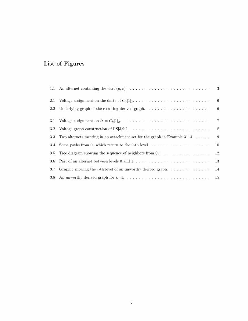
List of Figures

1.1 An alternet containing the dart (u, v). . . . . . . . . . . . . . . . . . . . . . . . . . . 3

2.1 Voltage assignment on the darts of C3[1]2. . . . . . . . . . . . . . . . . . . . . . . . . 6

2.2 Underlying graph of the resulting derived graph. . . . . . . . . . . . . . . . . . . . . 6

3.1 Voltage assignment on ∆ = Ck[1]2. . . . . . . . . . . . . . . . . . . . . . . . . . . . . 7

3.2 Voltage graph construction of PS[3,9;2]. . . . . . . . . . . . . . . . . . . . . . . . . . 8

3.3 Two alternets meeting in an attachment set for the graph in Example 3.1.4 . . . . . 9

3.4 Some paths from 00 which return to the 0-th level. . . . . . . . . . . . . . . . . . . . 10

3.5 Tree diagram showing the sequence of neighbors from 00. . . . . . . . . . . . . . . . 12

3.6 Part of an alternet between levels 0 and 1. . . . . . . . . . . . . . . . . . . . . . . . . 13

3.7 Graphic showing the i -th level of an unworthy derived graph. . . . . . . . . . . . . . 14

3.8 An unworthy derived graph for k=4. . . . . . . . . . . . . . . . . . . . . . . . . . . . 15

v

Chapter 1

Preliminaries

All graphs and groups in this paper are assumed to be finite. Let Γ be an arbitrary graph. An edge

of Γ is an unordered pair of vertices {u, v}. A dart is a directed edge or ordered pair of vertices

(u, v). We think of an edge {u, v} being the union of the two darts along that edge: (u, v) and (v, u).

We denote the vertex-set, edge-set and dart-set of Γ by V(Γ) , E(Γ) and D(Γ) respectively. The

valence of a vertex v ∈ V(Γ) is the number of edges incident to v. We then say Γ is regular provided

that every vertex of Γ has the same valence. In this case, if the valence of each vertex of Γ is d, we

say the graph is d-valent.

If for every edge {u, v} of Γ we choose one of the darts (u, v) or (v, u), the resulting collection of

darts is a directed graph (digraph) called an orientation ∆ of Γ. We say Γ is the underlying graph

of ∆. Also, we say ∆ is of valency d if its underlying graph Γ is d-valent. An in-neighbor of a vertex

v ∈ V(∆) is a vertex u such that (u, v) is an dart of ∆. Similarly, an out-neighbor of v is a vertex w

such that (v, w) is an dart of ∆. In this paper we consider directed regular multigraphs, where each

vertex has the same number of in-neighbors as out-neighbors. We say that a graph Γ is unworthy if

two or more distinct vertices of Γ share exactly the same neighbors. If Γ is not unworthy, it is said

to be worthy. An orientation is said to be unworthy (or worthy) if its underlying graph is unworthy

(or worthy). We say a graph Γ is connected if for each u, v ∈ V(Γ) there is a sequence of vertices

u = w0, w1, . . . , wm−1, wm = v such that wi and wi+1 are adjacent for i ∈ {0, 1, . . . ,m − 1}. A

digraph is said to be connected when its underlying graph is connected.

If a permutation of the vertices of Γ preserves its edges, we call it a symmetry, or automorphism,

of Γ. Collectively, the symmetries of Γ form a group under composition called the automorphism

group of Γ which is denoted Aut(Γ). Similarly, permutations of the vertices of an orientation ∆

that preserve the darts of ∆ form a group of symmetries, denoted Aut(∆). We say that Γ is vertex-

1

transitive if Aut(Γ) acts transitively on V(Γ). In other words, Γ is vertex-transitive if all of the

vertices of Γ are in the same orbit under the action of Aut(Γ). Similarly, Γ is edge-transitive or

dart-transitive provided Aut(Γ) acts transitively on E(Γ) or D(Γ) respectively. A semi-transitive

orientation of Γ is an orientation ∆ whose automorphism group acts transitively on the darts and

vertices of ∆. We say Γ is semi-transitive when it has a semi-transitive orientation. Furthermore, Γ

is 12 -transitive (or half-arc-transitive) if it has a semi-transitive orientation ∆ and Aut(Γ) = Aut(∆).

A semi-transitive graph Γ is 12 -transitive if and only if Aut(Γ) contains no dart-reversing symmetries.

We say the graph is dart-transitive if it is semi-transitive and Aut(Γ) acts transitively on all darts of

Γ. When showing a graph is semi-transitive, it is enough to show vertex-transitivity and to examine

the stabilizer of a vertex and the action on the out-neighbors of that vertex. Hence we have the

following theorem giving another description of semi-transitivity.

Theorem 1.0.1 Let ∆ be an orientation of a graph Γ, and G = Aut(∆). Then ∆ is a semi-

transitive orientation if and only if ∆ is vertex-transitive and for some v ∈ V(∆) the stabilizer Gv

of v is transitive on the out-neighbors of v.

Proof: (=⇒) This follows from the definition of a semi-transitive orientation.

(⇐=) Let (u, v), (x, y) ∈ D(∆). Note that by vertex-transitivity, if the condition on the stabilizer

holds at any vertex, it holds at every vertex. Then since ∆ is vertex-transitive there is a ρ ∈ Aut(∆)

such that uρ = x. Since ρ is an automorphism of ∆ it must send v to some out-neighbor y′ of x,

though y′ may not necessarily be y. If vρ = y′ = y then (u, v)ρ = (x, y). Suppose y′ &= y. Then

since Gx is transitive on the out-neighbors of x there is a σ ∈ Gx such that (x, y′)σ = (x, y). Thus

(u, v)ρσ = (x, y′)σ = (x, y), with ρσ ∈ Aut(∆). !

A k-cycle, denoted Ck, is a graph on k vertices with k edges where the vertex-set is Zk and the

edge-set is {{i, i+1} | i ∈ Zk}. If every edge is given the orientation (i, i+1) the resulting orientation

is called the directed k -cycle, denoted Ck[1]. Given an orientation ∆ we define the d-plicated oriented

graph of ∆, denoted ∆d, to be the digraph with vertex-set V(∆d) = V(∆). Intuitively, to obtain

∆d we replace each dart of the base graph ∆ with d parallel copies, having the same initial and

terminal vertices as the original dart. We then label the darts of the resulting multigraph as (u, v)j

where (u, v) is the original dart and j ∈ Zd. Clearly every directed k -cycle Ck[1] is graded for k ≥ 3.

Also, if an orientation ∆ has a k-grading, it has a k′-grading for every k′ dividing k. Note that C6[1]

has a 1-, 2- and 3-grading, but grade(C6[1]) = 6. We note that a digraph of grade k is therefore a

covering of a directed d-plicated k′-cycle, where k′|k, for some d ∈ N. This motivates a deeper study

in graph coverings, and so we turn to voltage constructions as presented in Chapter 2.

2

Recall from [6] and [7] the following terms:

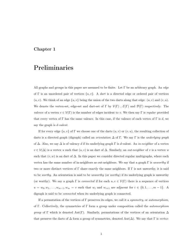
Definition 1.0.2 An alternet of an orientation ∆ of a semi-transitive graph Γ is a subdigraph of

∆ induced by a set of darts defined as follows: Begin with a dart (u, v) and let A1 be the set of all

darts with initial vertex u. Then let A2 be the set of all darts sharing the same terminal vertices

as those in A1. Let A3 then be the set of all darts sharing the same initial vertices as those in A2.

We recursively form the sets Ai in the same way. The alternet containing the dart (u, v) is then

A = ∪Ai.

We note that if the orientation is 4-valent the alternet is called an alternating cycle in [6]. See

Figure 1.1 below for an example of an alternet of a 4-valent orientation.

The head-set of an alternet Ax (denoted Hx) is the set of all terminal vertices of the darts in the

alternet, and similarly the tail-set of Ax (denoted Tx) is the set of all initial vertices of the darts in

the alternet.

We say that ∆ is tightly-attached if Hx = Ty for some x and y. An attachment set is a nonempty

intersection of some head-set Hx with some tail-set Ty. All attachment sets are of the same size, m.

If If m = 1 we say the graph is loosely-attached. If 1 < m < |Hx| for every x and y, then the graph

is said to be semi-attached.

Figure 1.1: An alternet containing the dart (u, v).

Let ∆ be an orientation of a graph Γ. Let k ∈ N. A k-grading of ∆ is a function f : V (∆) −→ Zk

such that for every dart (u, v) ∈ D(∆) we have f(v) ≡ f(u) + 1 (mod k). We say the grade of ∆,

denoted grade(∆), is the largest k such that ∆ has a k-grading. We note that every graph has a

1-grading. Similarly, every bipartite graph has a 2-grading. Finally, we say that ∆ is graded provided

that grade(∆) = k ≥ 3. If ∆ is graded, we say it is a graded orientation of its underlying graph Γ.

Examples of Graded Orientations

The following theorem provides a family of examples of tightly-attached graded semi-transitive

orientations.

3

Theorem 1.1 Suppose ∆ is a tightly-attached semi-transitive orientation of a graph Γ that has at

least three alternets. Then ∆ is graded.

Proof: See Section 7 of [7]. !

All tightly-attached semi-transitive orientations of valency 4 have been classified (see [5, 6]). The

objective of this paper is to present semi-attached graded semi-transitive orientations.

4

Chapter 2

Voltage Graphs

A covering projection p from a graph Γ′ onto a graph Γ is a mapping from V(Γ′) onto V(Γ) such

that, for every v ∈ V(G), the neighborhood of v′ is mapped bijectively onto the neighborhood of

v = p(v′) in Γ.

We say that Γ′ is a cover of Γ. Let ∆ be an orientation of Γ and let (u, v) ∈ D(∆). Let Γ′ be a

cover of Γ. Then for every edge {u′, v′} of Γ′, where p(u′) = u and p(v′) = v, we form the dart (u′, v′).

The resulting orientation is denoted ∆′, and we say ∆′ is a cover of ∆. As we will see, voltage graphs

are a special kind of covering graphs, in which the covering is more easily comprehended visually

than other covering techniques.

Let ∆, called the base graph, be an orientation of some graph Γ. Let A be a group, called the

voltage group. Let α : D(∆) −→ A be an ordinary voltage assignment. That is, α assigns an element

of A to each dart of ∆. In this paper we consider only finite Abelian groups for voltage groups. The

resulting graph is called an ordinary voltage graph, or just a voltage graph, and is denoted (∆, α).

We then construct the derived graph ∆α with vertex set V(∆α) = V(∆) × A. For v ∈ V(∆) and

a ∈ A we will use the notation va for vertices in V(∆α), instead of (v, a). Additionally, let (u, v) be

a dart of the base graph with voltage a ∈ A. Darts of ∆′ are of the form (ux, va+x) ∈ D(∆α) for

every x ∈ A and (u, v) ∈ D(∆).

Let W = (v0, v1, . . . , vn) be a walk of length n from vertex v0 to vertex vn in (∆, α). Then we

say the total voltage of W is∑n

i=1 α(ei), where ei is the dart from vi−1 to vi for i ∈ {1, . . . , n}. If

(vi−1, vi) is the reverse of some dart of ∆α we take α((vi−1, vi)) to be −α((vi, vi−1)). It is a fact

[see [3]] that walks with total voltage 0 in the base graph lift to closed walks in the derived graph.

Finally, we note that the voltage group A acts on the vertices of ∆α as a group of symmetries (called

the natural action of A in [3]). For example, let ix ∈ V(∆α) for some x ∈ A and let a ∈ A. Then

5

(ix)a = ix+a. It is not difficult to see that this action is transitive on each vertex fiber.

For an example of a voltage graph construction, consider Γ = (C3)2, the 2-plicated 3-cycle. Let

∆ = C3[1]2, A = Z3 and α : D(∆) −→ A be given by Figure 2.1 below. Then the resulting derived

graph has the underlying graph given in Figure 2.2.

Figure 2.1: Voltage assignment on the darts of C3[1]2.

Figure 2.2: Underlying graph of the resulting derived graph.

6

Chapter 3

Constructing Graded Semi-Transitive

Orientations

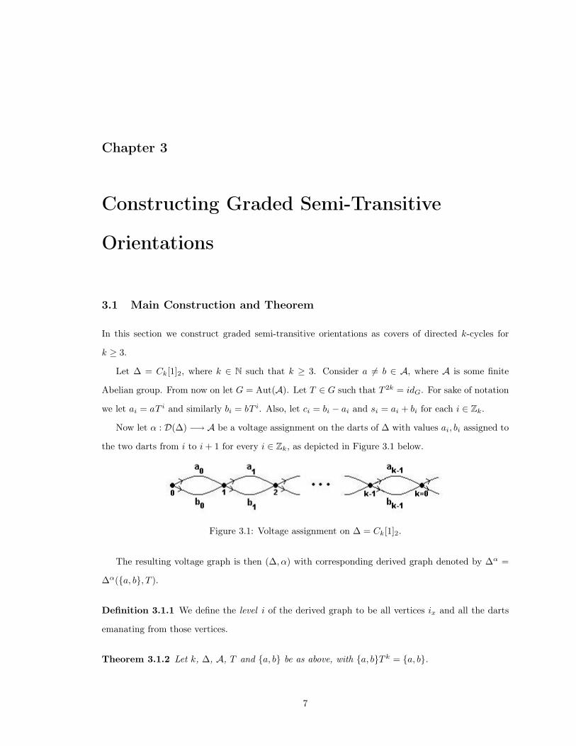
3.1 Main Construction and Theorem

In this section we construct graded semi-transitive orientations as covers of directed k-cycles for

k ≥ 3.

Let ∆ = Ck[1]2, where k ∈ N such that k ≥ 3. Consider a &= b ∈ A, where A is some finite

Abelian group. From now on let G = Aut(A). Let T ∈ G such that T 2k = idG. For sake of notation

we let ai = aT i and similarly bi = bT i. Also, let ci = bi − ai and si = ai + bi for each i ∈ Zk.

Now let α : D(∆) −→ A be a voltage assignment on the darts of ∆ with values ai, bi assigned to

the two darts from i to i + 1 for every i ∈ Zk, as depicted in Figure 3.1 below.

Figure 3.1: Voltage assignment on ∆ = Ck[1]2.

The resulting voltage graph is then (∆, α) with corresponding derived graph denoted by ∆α =

∆α({a, b}, T ).

Definition 3.1.1 We define the level i of the derived graph to be all vertices ix and all the darts

emanating from those vertices.

Theorem 3.1.2 Let k, ∆, A, T and {a, b} be as above, with {a, b}T k = {a, b}.

7

Further, suppose s0 ∈ ker(k−1∑

i=0

T i). Then we have the following for ∆α = ∆α({a, b}, T ):

1. ∆α is graded of grade k or 2k.

2. ∆α is connected if and only if C = 〈c0, c1, . . . , ck−1,k−1∑

i=0

ai〉 = A.

3. ∆α is a semi-transitive orientation.

4. The head-sets of ∆α are of size |〈c0〉| and the size of an attachment set is |〈c0〉 ∩ 〈c1〉|.

Therefore we have the following:

(a) ∆α is tightly-attached if and only if 〈c0〉 = 〈c1〉.

(b) ∆α is loosely-attached if and only if |〈c0〉 ∩ 〈c1〉| = 1.

(c) ∆α is semi-attached if and only if 1 < |〈c0〉 ∩ 〈c1〉| < |〈c1〉|.

5. The derived graph is unworthy in two cases:

(a) If k &= 4, ∆α is unworthy if and only if c0 = −c0 = c1 = −c1.

(b) If k=4, ∆α is unworthy if c0 = ±c1.

The proof of this theorem will occupy the remainder of this chapter. We first present several

examples of the construction and then proceed with the various proofs of the parts of the theorem.

Example 3.1.3 We construct the Power-Spidergraph family PS[k,M ; r]. Recall from [7] the con-

struction of the Power-Spidergraph PS = PS[k, M ; r]. The vertices of PS are labeled with elements

of the Cartesian product Zk × ZM . The darts of PS join each vertex (i, j) to vertices (i + 1, j ± ri).

With this orientation, PS is a semi-transitive orientation of its underlying graph [see [7]]. To

construct PS from a k-cycle, let ∆ = Ck[1]2 and A = ZM . Also, let T be given by multiplication

by r ∈ U(ZM ) with rk = ±1, where U(ZM ) is the group of units of ZM . Let a = 1 ∈ ZM and

b = −1 ∈ ZM . Then ∆α({a, b}, T ) = PS[k, M ; r]. See Figure 3.2 below to see an example of how to

construct PS[3, 9; 2] (note A = Z9).

Figure 3.2: Voltage graph construction of PS[3,9;2].

8

Again from [7] we have that the Power-Spidergraph family is tightly-attached. We now present

an example of a semi-attached graph.

Example 3.1.4 Let ∆ = C6[1]2 and A = Z3 ⊕ Z9. Let (x, y) ∈ A and let T ∈ G be defined by

the mapping (x, y) /−→ (2x,−2y). Then let a = (1, 1) ∈ A and b = (0, 5) ∈ A. Also, we have

that a1 = (2,−2) = (2, 7) and b1 = (0, 8). Then the orientation ∆α is indeed a semi-transitive

orientation on 162 vertices and 324 darts. In fact, its underlying graph Γ′ is 12 -transitive, since

|Aut(Γα)| = |Aut(∆α)| = 324, as given by a MAGMA [2] calculation. It is worthwhile to note that

if k = 3 then the derived graphs are dart-transitive, again verified by MAGMA.

Note that c0 = b0 − a0 = (2, 4) and c1 = c0T = (1, 1). Then we see that |〈c0〉| = 9 and

|〈c0〉 ∩ 〈c1〉| = |〈(0, 3)〉| = 3. Thus ∆α = ∆α({a, b}, T ) is a semi-attached graded orientation with

head-sets of size 9 and attachment sets of size 3. See Figure 3.3 below for a visual of an attachment

set at level 1. The three rows of vertices shown consist of 3 groups of 9 vertices. The labeling of

the first group in the top row is given by, from left to right, 0(0,0), 0(0,1), . . . , 0(0,8). The labeling of

the next two groups is given by 0(1,x) and 0(2,x) where x ∈ Z9 is given in the same order as the

first group. The groups of vertices in the second row are labeled similarly as 1(0,x), 1(1,x) and 1(2,x).

Finally, the groups of vertices in the third row are labeled as 2(0,x), 2(1,x) and 2(2,x) with x ∈ Z9

given in the same order as the previous rows. Also in the figure we see an alternet between levels

0 and 1 containing the vertex 0(0,0) and an alternet between levels 1 and 2 containing the vertex

1(1,0). These two alternets meet in the attachment set {1(0,2), 1(0,5), 1(0,8)}, which is seen in the first

group of vertices in the second row of the figure.

Figure 3.3: Two alternets meeting in an attachment set for the graph in Example 3.1.4

9

3.2 Proof of Theorem 3.1.2

Proof: (1). The fact that ∆α is graded follows directly from the construction. Also, we note

that walks with total voltage 0 = 0A must lift to closed walks in the derived graph. Since s0 ∈

ker(∑k−1

i=0 T i) we have that∑k−1

i=0 ai +∑k−1

i=0 bi = 0A, and so it follows that the grade of the derived

graph must be no more than the length of the walk starting at a vertex and traversing all the ai-

darts, followed by the bi-darts. That is, k′ = grade(∆α) ≤ 2k. Since the orientation was originally

given a k-grading, it must be that the grade of the derived graph is a multiple of k. Hence k′ = k

or k′ = 2k. !

Figure 3.4: Some paths from 00 which return to the 0-th level.

We now show part (2) of Theorem 3.1.2, that is, we determine when ∆α is connected. To do this

we start at a vertex and find all possible paths from that vertex back to the same level containing

that vertex. Without loss of generality we consider 00 ∈ V(∆α). We first consider paths that traverse

darts in the positive direction from level 0 to some level i, and then traverse darts in the negative

direction back to level 0. From Figure 3.4 above we see that if we go out to level 2, 0x is in the

same component as 00 for every x ∈ 〈c0, c1〉. Including paths out to level 3 we have that 0x is in

the same component as 00 for every x ∈ 〈c0, c1, c2〉. Continuing to include paths out to include

vertices in the k-th level (0-th level), we have that 0x is in the same component as 00 for every

x ∈ 〈c0, c1, . . . , ck−1〉. We note, however, that we can also reach the 0-th level from 00 by traversing

every dart in the positive direction with label ai for each i. Thus, we have that 0x is in the same

component as 00 if and only if x ∈ C = 〈c0, c1, . . . , ck−1,∑k−1

i=0 ai〉. Any path beginning at level 0

and ending at level 0, passing through levels 1, 2, 3, . . . , k−1 differs in voltage from a path consisting

only of ai-darts by a sum of ci’s, and so its total voltage is in C.

10

Since ci = bi − ai and∑k−1

i=0 ai ∈ C, we need not consider paths traversing darts with labels bi.

Following convention in [3], we say that C is the local group at 00 (and so at every vertex

v ∈ V(∆α) since A is Abelian). Corollary 2 to Theorem 2.5.1 in [3] states that the number of

components of the derived graph is the index of the local group in the voltage group. Applying this

fact to the construction of this paper gives the following theorem.

Theorem 3.2.1 There are [A : C] components of the derived graph.

Therefore we have that ∆α is connected if and only if the local group C is exactly the voltage group

A and so Theorem 3.1.2 (2) follows.

From now on we assume ∆α is connected. We now wish to show part (3), that is, to show when

∆α is semi-transitive. Recall that an orientation is a semi-transitive orientation provided that its

automorphism group acts transitively on the vertices and darts of the orientation. In order to apply

Theorem 1.0.1 to our construction we first consider the rotation symmetry ρ ∈ Aut(∆) defined by

iρ = i + 1.

Then ρ lifts as a symmetry ρ ∈ Aut(∆α), where ρ is given by

ixρ = (iρ)xT = (i + 1)xT ∈ V(∆α).

To see that ρ is indeed a symmetry of the derived graph, consider, without loss of generality

consider the dart (ix, (i + 1)x+ai) ∈ D(∆α). Then (ix, (i + 1)x+ai)ρ = ((iρ)xT , ((i + 1)ρ)(x+ai)T ) =

((i + 1)xT , (i + 2)xT+ai+1) ∈ D(∆α). Thus ρ ∈ Aut(∆α). Then since the natural action of the

voltage group is transitive on the fibers over each vertex in ∆, we have that ∆α is vertex-transitive.

Thus we need only consider the stabilizer of some vertex in ∆α. Without loss of generality consider

00 ∈ V(∆α) and examine Figure 3.5 below. With the ai-darts being the ”up” darts and the bi-

darts being the ”down” darts, we see that the vertices on the far right of the figure, from top to

bottom, have labels 0Pk−1i=0 ai

, 0Pk−1i=0 δiai+

Pk−1i=0 ζibi

and 0Pk−1i=0 bi

, respectively, where δi, ζi ∈ {0, 1}

and δi + ζi = 1. From now on let Aj =j∑

i=0

ai and Bj =j∑

i=0

bi.

Let Si =∑i−1

j=0 sj with it understood that S0 is the empty sum; that is, S0 = 0. Then S1 = s0 ∈

ker(∑k−1

i=0 T i). Then for every i ∈ Zk and x ∈ A we define the symmetry σ at the i-th level by

ixσ = iSi−x.

11

Figure 3.5: Tree diagram showing the sequence of neighbors from 00.

Thus for i = 0 we have that 0xσ = 00−x = 0−x. The definition of this symmetry is motivated by

the fact that s0 ∈ ker(∑k−1

i=0 T i), and so∑k−1

i=0 ai = −∑k−1

i=0 bi. The action by σ can be viewed as a

reflection about the horizontal line passing through 00, bisecting the tree in Figure 3.5.

We note that this σ may not be the only symmetry that has this property, but for the sake of

this paper we only consider this symmetry.

Lemma 3.2.2 Let σ be defined as above. Then σ ∈ Aut(∆α).

Proof: We first let (ix, (i + 1)x+ai) ∈ D(∆′), for i ∈ {0, . . . , k − 2} and some x ∈ A. Then

(ix, (i + 1)x+ai)σ = (ixσ, (i + 1)x+aiσ) =(iSi−x, (i + 1)Si+1−(x+ai)) = (iSi−x, iSi−x+bi) ∈ D(∆′).

Similarly, (ix, (i + 1)x+bi)σ ∈ D(∆′). Now consider i = k − 1. Then ((k − 1)x, 0x+ak−1)σ = ((k −

1)xσ, 0x+ak−1σ) = ((k−1)Sk−1−x, 0−x−ak−1). Here we note that since s0 ∈ ker(∑k−1

i=0 T i) we have that

Sk =∑k−1

i=0 si = s0∑k−1

i=0 T i = 0. Thus ((k− 1)Sk−1−x, 0−x−ak−1) = ((k− 1)Sk−sk−1−x, 0−x−ak−1) =

((k−1)0−sk−1−x, 0−x−ak−1) = ((k−1)−ak−1−bk−1−x, 0−x−ak−1) ∈ D(∆′). Similarly, ((k−1)x, 0x+bk−1)σ ∈

D(∆α). !

We are now ready to prove Theorem 3.1.2 (3).

Proof: (3). This proof follows from the construction and the existence of the symmetry σ of Lemma

3.2.3. Let G = Aut(∆α). Let σ ∈ G be defined as above. We have that G acts transitively on the

vertices of ∆α. Then for 00 ∈ V(∆α) we have σ ∈ G00 where G00 " G is the stabilizer of 00. Then

for 1a0 and 1b0 , the two out-neighbors of 00, we have 1a0σ = 1S0−a0 = 1s0−a0 = 1b0 . Similarly, we

have 1b0σ = 1a0 . Hence by Theorem 1.0.1 we have that ∆α is a semi-transitive orientation of its

underlying graph. !

12

We now turn to the discussion of attachment sets.

Figure 3.6: Part of an alternet between levels 0 and 1.

Examining Figure 3.6 we see that the tail-set of the alternet between levels 0 and 1 including

the vertex 00 is the set {0〈c0〉}. In general, tail-sets of the alternets between levels 0 and 1 are

formed by cosets of 〈c0〉. Similarly, tail-sets at level i are formed by cosets of 〈ci〉. To look at

the possible attachment sets, consider the vertex ix ∈ V(∆α). Then the tail-set containing that

vertex is the set {ix+〈ci〉}. Then an in-neighbor of ix is (i−1)x−ai−1 , which has out-neighbors ix and

ix−ai−1+bi−1 = ix+ci−1 . Extending this, we see that the head-set of the alternet based at (i−1)x−ai−1

is the set {ix+〈ci−1〉}. Thus the attachment sets at level i are of the form {ix+〈ci〉∩〈ci−1〉|x ∈ A}.

Since ∆α is vertex-transitive we need only consider i = 1. Hence we see that the derived graph

is tightly-attached precisely when 〈c0〉 = 〈c1〉, loosely-attached if and only if |〈c0〉 ∩ 〈c1〉| = 1 and

semi-attached precisely when 1 < |〈c0〉 ∩ 〈c1〉| < |〈c1〉|. Thus we have Theorem 3.1.2 (4).

We now wish to find the requirements on the voltage assignment that will yield an unworthy

derived graph, in order to prove Theorem 3.1.2 (5). Recall that we say an orientation ∆ is unworthy

if its underlying graph is unworthy. Consider orientations ∆ as constructed in this paper, with

underlying graphs Γ. Then for two vertices u, v ∈ V(∆), if they have the same neighbors in Γ, one

of two possibilities can occur: (a) u and v are in the same level i, or (b) u is in some level i and v

is in some level i + 2.

For Case (a), we consider two vertices ix and ix′ of the derived graph, where i ∈ Zk and

x &= x′ ∈ A, and consider the in- and out-neighbors of each vertex as seen in Figure 3.7.

Proof: [5 (a)] (⇒) From Figure 3.7 we see that if the derived graph is unworthy then it must be that

13

Figure 3.7: Graphic showing the i -th level of an unworthy derived graph.

x′ + ai = x + bi and x′ + bi = x + ai, since x &= x′ and ai &= bi. Thus x + bi − ai = x′ = x + ai − bi.

Hence ci = −ci. Similarly, we must have that x′ − bi−1 = x− ai−1 and x′ − ai−1 = x− bi−1, which

implies that x + bi−1 − ai−1 = x′ = x + ai−1 − bi−1. Hence ci−1 = −ci−1, but clearly x′ = x′ and so

from the two previous results we have ci−1 = −ci−1 = ci = −ci. Since i was arbitrary, this must be

true for every i ∈ Zk. Thus we need only consider i = 1.

(⇐) Suppose c0 = −c0 = c1 = −c1 and consider the vertices 1x and 1x+c1 for some x ∈ A. Then

the two out-neighbors of 1x are 2x+a1 and 2x+b1 . Since c1 = −c1 we have that c1 + a1 = b1 and

c1 + b1 = b1− c1 = a1. Thus the two out-neighbors of 1x+c1 are also 2x+b1 and 2x+a1 . Now, the two

in-neighbors of 1x are 0x−a0 and 0x−b0 . Since c1 = c0 = −c0 we have that x + c1 = x + c0 = x− c0

and so the two in-neighbors of 1x+c1 = 1x+c0 = 1x−c0 are 0x−a0 and 0x−b0 . Therefore 1x and 1x+c1

have exactly the same in- and out-neighbors, and so the derived graph is unworthy. !

Now, in Case (b), we note the only way that two vertices in the underlying derived graph can

share common neighbors and not be in the same fiber is if k = 4. Then it must be that some vertex

ix has as its out-neighbors the in-neighbors of some (i + 2)x′ and vice-versa, for some x, x′ ∈ A

(see Figure 3.8 below). We note the in-neighbors of ix are (i − 1)x−ai−1 and (i − 1)x−bi−1 , and

the out-neighbors of ix are (i + 1)x+ai and (i + 1)x+bi . Similarly, the in-neighbors of (i + 2)x′ are

(i+1)x′−ai+1 and (i+1)x′−bi+1 , and the out-neighbors of (i+2)x′ are (i+3)x′+ai+2 and (i+3)x′+bi+2 .

Proof: [5 (b)] (⇒) This proof is split into the following two cases:

Case 1: x− ai−1 = x′ + ai+2 and x− bi−1 = x′ + bi+2.

We have x′ = x− ai−1 − ai+2 = x− bi−1 − bi+2 and so ci = −ci+3. Hence c0 = −c1.

14

Figure 3.8: An unworthy derived graph for k=4.

Case 2: x− ai−1 = x′ + bi+2 and x− bi−1 = x′ + ai+2.

We have x′ = x− ai−1 − bi+2 = x− bi−1 − ai+2 and so ci = ci+3. Hence c0 = c1.

Thus we see that from these two cases, the derived graph is unworthy if c0 = ±c1. !

Remark 3.2.3 If∑k−1

i=0 T i = 0E , where E is the ring of endomorphisms ofA, then ker(∑k−1

i=0 T i) = A

and so any voltage assignment with image {a, b} ⊆ A at level 0 will yield a semi-transitive derived

graph. However, the graphs may be unworthy and/or disconnected. Since any voltage assignment

will work, we can choose a = 0 ∈ A and b ∈ A arbitrary.

15

Chapter 4

Special Families of Graded Semi-Transitive

Orientations

As seen in Example 3.1.3, we can construct the Power-Spidergraph family PS[k, M ; r] using the

method presented in this paper. This 4-valent family consists of graded semi-transitive orientations,

most of which are 12 -transitive [see [6], [7]].

We now present two constructions of graded semi-transitive orientations that are more general

than the 4-valent constructions presented in Chapter 3.

Consider the family of directed wreath graphs W [N, k] and the family of directed depleted wreath

graphs DW [N, k]. The directed wreath graphs are digraphs on k ·N vertices, where the vertices are

arranged in N ”rings” and k ”spokes” in which each vertex of each spoke i is connected by a dart

to every vertex in spoke i + 1. That is, darts of W [N, k] are of the form (ij , (i + 1)l) where i ∈ Zk,

for every j, l ∈ ZN . Similarly, the directed depleted wreath graphs are digraphs on k ·N vertices in

which the vertices are arranged in N ”rings” and k ”spokes”. However, here each vertex v of each

spoke i is connected by a dart to every vertex in spoke i + 1 except for the vertex in the same ring

as v. That is, darts of DW [N, k] are of the form (ij , (i + 1)l) where i ∈ Zk, for each j ∈ ZN and

every l ∈ ZN \ {j}. We note that the directed wreath and depleted wreath graphs are graded for

k ≥ 3, and so we wish to show that these families of graphs are a special case of the construction

presented in this paper. To that end, let A be a finite Abelian group and let N = |A|. Also, let

G = Aut(A), T = idG and k ≥ 3. We note that the isomorphism classes are dependent only on |A|

in each theorem.

Theorem 4.1 (Directed wreath graphs) Let ∆ = Ck[1]N , and let α : D(∆) −→ A be surjective at

each level. The resulting derived graph is then isomorphic to W [N, k].

16

Theorem 4.2 (Directed depleted wreath graphs) Let ∆ = Ck[1]N−1, and let α : D(∆) −→ A\ {0}

be surjective at each level. The resulting derived graph is then isomorphic to DW [N, k].

17

Chapter 5

Extending the Results to Graphs of Valency

4(pn − 1)

We now use the Galois voltage technique given in Section 6 of [1] to extend the results of this paper

to graded semi-transitive orientations of valency 4(pn − 1) for primes p and n ∈ N.

Theorem 5.0.4 Let ∆ be a graded semi-transitive orientation of valency 4 as constructed in this

paper. Let A = Znp for some prime p and n ∈ N. Let O = ∆d where d = pn−1 and let α : D(O) −→

A \ {0} be bijective at every dart of ∆, where 0 = Id ∈ A. Then the derived graph Oα is a graded

semi-transitive orientation of valency 4(pn − 1). Furthermore, we have the following:

1. Oα is graded.

2. If ∆ is connected then Oα is connected.

3. If ∆ is worthy then Oα is worthy.

4. If ∆ is tightly-, loosely- or semi-attached then Oα is tightly-, loosely- or semi-attached respec-

tively.

Proof: This follows from the fact that Znp is the additive group of GF (pn) and so the multiplicative

group G′ of GF (pn) is cyclic and acts on A \ {0} cyclically. Let G′ = 〈γ〉. Then γ acts transitively

on A \ {0} and is the symmetry required for the use of Theorem 1.0.1. The fact that Oα is graded

follows from the construction, as the levels are inherited through the fibers. Parts 2 and 3 of the

theorem are trivial. We have part 4 since the covering preserves the structure of the attachment

sets, increasing only the size of each head-set, tail-set and attachment set by |A|. !

Note that if p = 2 and n = 1 we see that the derived graph is the bipartite double cover of the base

graph.

18

Chapter 6

Open Questions

The main open question relating to this paper is the matter of when two derived graphs are isomor-

phic given two different voltage assignments on the base graph. The following section sheds some

light on the subject.

Isomorphisms

Let ∆ = Ck[1]2 and let A, k ≥ 3 and T be given as above. Let a0, b0, a′0, b′0 ∈ A and α1 : D(∆) −→ A

and α2 : D(∆) −→ A have images {a0, b0} and {a′0, b′0} at level 0 respectively. Clearly ∆α1 ∼= ∆α2

if {a0, b0} = {a′0, b′0}.

We now present a theorem from [5] stating when two derived graphs (arising from different

voltage assignments) are isomorphic with respect to a subgroup of the symmetry group of the base

graph. Let G = Aut(∆).

Definition 6.0.5 C0(∆,A) = {f : V(∆) −→ A}.

Definition 6.0.6 Let H " G. Two coverings p1 : ∆α1 −→ ∆ and p2 : ∆α2 −→ ∆ are isomorphic

with respect to H if there is a graph isomorphism Φ from ∆α1 to ∆α2 and a γ ∈ H such that

γ ◦ p1 = p2 ◦ Φ.

Theorem 6.0.7 (see [5]) Two A-coverings ∆α1 and ∆α2 are isomorphic with respect to H " G if

and only if there exist γ ∈ H, S ∈ Aut(A) and a function f ∈ C0(∆;A) such that

α2(eγ)f(i) = (α1(e))Sf(i + 1)

for every e ∈ D(∆), where e is a dart between levels i and i + 1.

19

We note that symmetries in the base graph are either powers of ρ (from Chapter 3), local "flips"

exchanging a ai-dart with a bi-dart at some level i, or some composition of powers of ρ and flips.

Now suppose two derived graphs ∆α1 and ∆α2 are isomorphic. Let e ∈ D(∆) be a dart emanating

from level i with voltage ai and let γ ∈ H " G. Then, by Theorem 6.0.9, it must be that for some

f ∈ C0(∆;A) and some S ∈ Aut(A) we have a′jf(i) = aiSf(i + 1) or b′jf(i) = aiSf(i + 1). Here, a′j

and b′j are the values of α2 on the two darts at level j in ∆α2 , one of which is the image of e under

γ.

Theorem 6.0.9 states when two coverings are isomorphic with respect to a subgroup of the auto-

morphism group and not as when isomorphic as graphs. Here we state an unsolved problem with

this construction.

Problem 6.0.8 Given ∆, A, T ∈ Aut(A) and two voltage assignments α1 and α2 on ∆ with images

{a, b} ⊆A and {a′, b′} ⊆A at the 0-th level respectively, what are the conditions so that ∆α1 ∼= ∆α2?

That is, how can we use Theorem 6.0.9 to show when two derived graphs are isomorphic?

We also note that the same T may produce non-isomorphic graphs. For instance, consider ∆ = C3[1]2

and A = Z3 × Z9. Let T be given by the mapping (x, y) /−→ (2x, 3x + 5y). Then for a = (1, 1) ∈ A

and b = (0, 8) ∈ A we have that ∆α({a, b}, T ) is connected, tightly-attached and 12 -transitive with

girth = 6, as given by MAGMA calculations. However for a′ = (1, 2) ∈ A and b′ = (0, 7) ∈ A we

have that ∆α({a′, b′}, T ) is connected, tightly-attached and dart-transitive with girth = 4, again

from MAGMA. We note that, in this example, s0 = (1, 0) = s′0 but c0 = (2, 7) &= (2, 5) = c′0.

Other Problems

Research also continues on the following topics:

1. What are the requirements on T so that the derived graph is dart-transitive? Similarly, what

are the requirements on T so that the derived graph is 12 -transitive? We note that a derived

graph is 12 -transitive provided that the covering is stable. That is, provided that there are no

"unexpected" symmetries that do not arise from a lift of a symmetry of the base graph or an

action of the voltage group on the fibers.

2. Can we classify the special families of derived graphs that arise when T = idG? Similarly, can

we classify those families arising from automorphisms T of order j where j|k? What are the

conditions, in either case, on {a, b} so that the derived graph is semi-transitive, connected,

20

worthy? What are the conditions required to construct tightly-, loosely- and semi-attached

graphs?

3. Can we construct graded semi-transitive orientations using non-Abelian voltage groups? For

example, what known graphs arise using voltage groups A = Sn, An or Dn?

4. Can the Mutant Power-Spidergraphs be constructed as in this paper? They make up a family

of graded semi-transitive orientations of valency 4 (see [7]).

5. What 4-valent circulant graphs can be constructed using the methods presented in this paper?

6. What graphs arise from other symmetries σ′ that fix 00? For example, let ∆ = C3[1]2,

G = Aut(A), A = Z8, T = idG, and a = 1, b = 3. We note in this case that s0 &∈ ker(k−1∑

i=0

T i).

In this (these) case(s) we have a different requirement on a, b so that the derived graph is

semi-transitive. Also, using the Chinese Remainder Theorem we can label the vertices of

∆α({a, b}, T ) to get ∆′ = C24[1, 5], the circulant graph on 24 vertices with vertex-set V(∆′) =

Z24 and darts of the form (i, i + 1) and (i, i + 5). Here, σ′ acts by

ixσ′ = i3x.

Consider the vertex 00 ∈ V(∆α). Then the tail-set in ∆α at level 0 containing the vertex 00

is the set {0x|x ∈ Z8 is even}. Similarly, the head-set in ∆α at level 1 containing the vertex

11 (an out-neighbor of 00) is the set {1y|y ∈ Z8 is odd}. We also see that for x ∈ Z8, where x

is even, xσ′ = 3x = −x. Thus, in a sense, this σ′ acts similarly to the symmetry σ of Lemma

3.2.2. We wish to generalize this result to other σ ∈ Aut(A).

7. Can we construct graded semi-transitive graphs of arbitrary valency d, where d &= 4(pn − 1)

(i.e. for d = 3, 5, 6, 7, . . .)? We may wish to turn to permutation voltage assignments, as they

allow a generalization of ordinary voltage assignments.

8. Given a base graph ∆ and voltage group A, what is the minimum (and maximum) number

of voltages we can assign at level 0 so that the derived graph is semi-transitive? Can we find

similar bounds to construct a 12 -transitive derived graph?

21

Chapter 7

Appendix

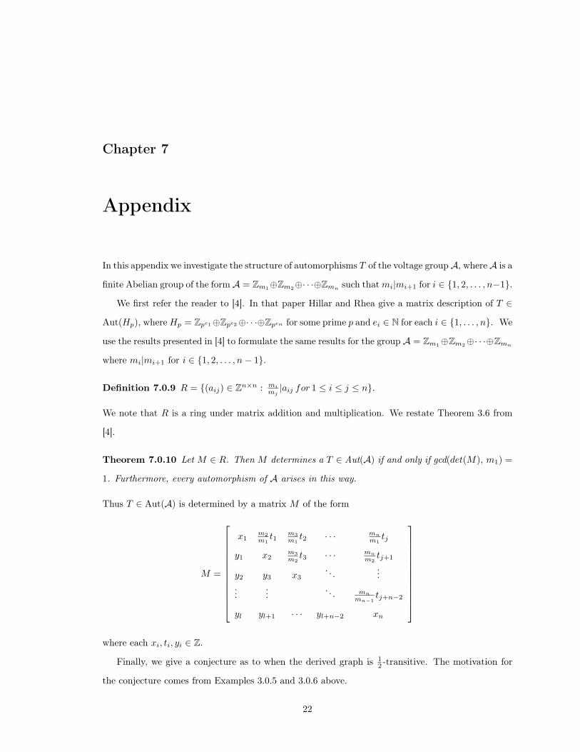
In this appendix we investigate the structure of automorphisms T of the voltage groupA, where A is a

finite Abelian group of the form A = Zm1⊕Zm2⊕· · ·⊕Zmn such that mi|mi+1 for i ∈ {1, 2, . . . , n−1}.

We first refer the reader to [4]. In that paper Hillar and Rhea give a matrix description of T ∈

Aut(Hp), where Hp = Zpe1⊕Zpe2⊕· · ·⊕Zpen for some prime p and ei ∈ N for each i ∈ {1, . . . , n}. We

use the results presented in [4] to formulate the same results for the group A = Zm1⊕Zm2⊕· · ·⊕Zmn

where mi|mi+1 for i ∈ {1, 2, . . . , n− 1}.

Definition 7.0.9 R = {(aij) ∈ Zn×n : mimj

|aij for 1 ≤ i ≤ j ≤ n}.

We note that R is a ring under matrix addition and multiplication. We restate Theorem 3.6 from

[4].

Theorem 7.0.10 Let M ∈ R. Then M determines a T ∈ Aut(A) if and only if gcd(det(M), m1) =

1. Furthermore, every automorphism of A arises in this way.

Thus T ∈ Aut(A) is determined by a matrix M of the form

M =

x1m2m1

t1m3m1

t2 · · · mnm1

tj

y1 x2m3m2

t3 · · · mnm2

tj+1

y2 y3 x3. . .

......

.... . . mn

mn−1tj+n−2

yl yl+1 · · · yl+n−2 xn

where each xi, ti, yi ∈ Z.

Finally, we give a conjecture as to when the derived graph is 12 -transitive. The motivation for

the conjecture comes from Examples 3.0.5 and 3.0.6 above.

22

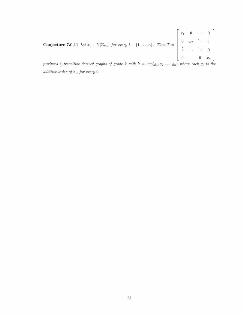
Conjecture 7.0.11 Let xi ∈ U(Zmi) for every i ∈ {1, . . . , n}. Then T =

x1 0 · · · 0

0 x2. . .

......

. . . . . . 0

0 · · · 0 xn

produces 12 -transitive derived graphs of grade k with k = lcm(g1, g2, . . . , gn) where each gi is the

additive order of xi, for every i.

23

Bibliography

[1] C. Attebery, Constructions of Symmetric and Semi-Symmetric Graphs Using Galois VoltageCovers, Preprint.

[2] W. Bosma, J. Cannon, and C. Playoust, “The MAGMA algebra system I: The user language”,J. Symbolic Comput. 24 (1997), 235Ð265.

[3] J. L. Gross, T. W. Tucker, “Topological Graph Theory”, Dover, New York, 2001.

[4] C. J. Hillar, D. L. Rhea, Automorphisms of Finite Abelian Groups. Preprint,arXiv:math/0605185v1.

[5] S. Hong, J.H. Kwak, J. Lee, Regular Graph Coverings Whose Covering Transformation GroupsHave The Isomorphism Extension Property, Discrete Math. 148 (1996), 85-105.

[6] D. Marusic, Half-Transitive Group Actions on Finite Graphs of Valency 4, J. Combin. TheorySer. B 73 (1998), 41-76.

[7] S. Wilson, Semi-transitive Graphs, J. Graph Theory 45 (2003), 1-27.

24