Semi-analytical Approximation for Solving High-order … · Semi-analytical Approximation for Solving High-order ... where lim k!1 k = 1and each ... both in classical mechanics and

British Journal of Mathematics & Computer Science4(23): 3345-3357, 2014

ISSN: 2231-0851

SCIENCEDOMAIN internationalwww.sciencedomain.org

Semi-analytical Approximation for Solving High-orderSturm-Liouville Problems

A. H. S. Taher∗1, A. Malek2 and A. S. A. Thabet11Department of Mathematics, University of Aden, P.O. Box: 205, Al-Habilain, Aden, Yemen.

2Department of Applied Mathematics, Faculty of Mathematical Sciences, Tarbiat Modares University,P.O. Box: 14115-134, Tehran, Iran.

Article InformationDOI: 10.9734/BJMCS/2014/13503

Editor(s):(1) Tian-Xiao He, Department of Mathematics and Computer Science, Illinois Wesleyan University,

USA.Reviewers:

(1) Anonymous, University of Guadalajara, Mexico.(2) Muhammad Amer Latif, Department of Mathematics, University of Hail, Saudi Arabia.

(3) Evgeny Nikulchev, Research Department, Moscow Technological Institute, Russia.Peer review History: http://www.sciencedomain.org/review-history.php?iid=669id=6aid=6299

Original ResearchArticle

Received: 19 August 2014Accepted: 08 September 2014

Published: 01 October 2014

AbstractIn this paper, an algorithm for solving high-order non-singular Sturm-Liouville eigenvalue problemsis proposed. A modified form of Adomian decomposition method is implemented to provide a semi-analytical solution in the form of a rapidly convergent series. Convergent analysis and error estimatebased on the Banach fixed-point is discussed. Five high-order Sturm-Liouville problems are solvednumerically. Numerical results demonstrate reliability and efficiency of the proposed scheme.

Keywords: High-order Sturm-Liouville problems; Modified Adomian decomposition method; Banachfixed point theorem; Eigenvalues; Eigenfunctions.2010 Mathematics Subject Classification: 34B24; 47H10; 34L10; 34L15; 34L16; 35C10

1 IntroductionIn this study, we will propose an alternative semi-analytical approximation based on a new type ofmodified Adomian decomposition which is an application of the fixed point iteration method to solve

*Corresponding author: E-mail: [email protected]

www.sciencedomain.org

British Journal of Mathematics and Computer Science 4(23), 3345-3357, 2014

non-singular high-order Sturm-liouville problems in the form

(−1)m(pm(x)y(m))(m) + (−1)m−1(pm−1(x)y(m−1))(m−1)

+ · · ·+ (p2(x)y′′)′′ − (p1(x)y

′)′ + p0(x)y = λw(x)y, a = 0 < x < b,(1.1)

subject to some 2m point specified conditions at the boundary x ∈ {a, b} on

uk = y(k−1), 1 ≤ k ≤ m,v1 = p1y

′ − (p2y′′)′ + (p3y

′′′)′′ + · · ·+ (−1)m−1(pmy(m))(m−1),

v2 = p2y′′ − (p3y

′′′)′ + (p4y(4))′′ + · · ·+ (−1)m−2(pmy

(m))(m−2),...vk = pky

(k) − (pk+1y(k+1))′ + (pk+2y

(k+2))′′ + · · ·+ (−1)m−k(pmy(m))(m−k),...vm = pmy

(m).

(1.2)

In Eq. (1.1), we assume that all coefficient functions are real valued. The technical conditions for theproblem to be non-singular are: the interval (a, b) is finite; the coefficient functions pk (0 ≤ k ≤ m−1),w(x) and 1/pm(x) are in L1(a, b), pm(x) and weight function w(x) are both positive. The eigenvaluesλk, k = 1, 2, 3, . . . can be ordered as an increasing sequence

λ1 ≤ λ2 ≤ λ3 ≤ · · · ,where lim

k→∞λk = ∞ and each eigenvalue has multiplicity at most m [1], [2]. The Sturm-Liouville

boundary value problems play an important role in both theory and applications of ordinary differentialequations. Many physical phenomena, both in classical mechanics and in quantum mechanics aredescribed mathematically by second-order Sturm-Liouville problems [3], [4], [5]. However manyimportant phenomena occurring in various fields of science are described mathematically by high-order Sturm-Liouville problems. For example, the free vibration analysis of beam structures [6], [7],[8] is governed by a fourth-order Sturm-Liouville problem, and it is known that when a layer of fluidis heated from below and is subject to the action of rotation, instability may set as overstability, thisinstability my be modelled by a eighth-order Sturm-Liouville boundary value problem with appropriateboundary conditions specified. It may be noted that, when instability sets as ordinary convection, themarginal state will be characterized by sixth-order Sturm-Liouville boundary value problem [9], [10],[11], [12]. Ten and twelfth-order Sturm-Liouville boundary value problems arise in the context whena uniform magnetic field is applied across the fluid in the same direction as gravity. When instabilitysets in as an ordinary convection, it is modelled by the tenth-order boundary value problems, wheninstability sets in as overstability, it is modelled by the twelfth-order boundary value problems [1], [2],[11], [12]. Let L2

w(a, b), be the space of functions f(x) on (a, b) such that∫ b

a

f(x)|2 w(x)dx <∞.

L2w(a, b) is a Hilbert space with inner product

〈f, g〉 =∫ b

a

f(x)g(x)w(x)dx,

and norm ‖f‖2 = 〈f, f〉. The standard Adomian decomposition method is applied for computingeigenvalues of Sturm-Liouville problems [13], [14], [15]. In the present work, based on basic ideaof the Adomian decomposition method [16], [17], [18] and [19], we will improve a modified Adomiandecomposition algorithm to solve high-order Sturm-Liouville problem (1.1) which is summarized inthe following section. The paper is organized as follows: Modified Adomian decomposition methodfor solving high-order Sturm-Liouville problems is proposed in Section 2. Whill convergence of a newmodification is discussed in Section 3. To illustrate the efficiency of proposed technique five numericalexamples are discussed in Section 4. Section 5 concludes the paper.

3346


2 Modified Adomian Decomposition Method (MADM)Let us rewrite equation (1.1) in the following form

(−1)m(pm(x)y(m))(m) = F (y, y′, . . . , y(2m−2), λ) = (λw(x)− p0(x))y−{(−1)m−1(pm−1(x)y)

(m−1) + · · ·+ (p2(x)y′′)′′}, a < x < b,

(2.1)

which can be written in the operator form as

Ly(x) +Ry(x) = 0, (2.2)

where Ly(x) = (pm(x)y(m))(m) and Ry(x) = −F (y, y′, . . . , y(2m−1), λ), Ry is a differential operatorsatisfies Lipchitz condition for y, y ∈ L2

w(a, b) and C > 0, we have, ‖Ry−Ry‖ ≤ C‖y− y‖. We definethe differential operator

L =dm

dxm

(pm(x)

dm

dxm

), (2.3)

then Eq. (2.1) can be rewritten as

Ly = F (y, y′, . . . , y(2m−2), λ), (2.4)

The inverse operator L−1 is therefore considered a 2m-fold integral operator defined by

L−1 =

∫ x

0

∫ x1

0

. . .

∫ xm−1

0︸︷︷︸m times

1

pm(xm)

∫ xm

0

∫ xm+1

0

. . .

∫ x2m−1


dx2m . . . dx1 (2.5)

Operating with L−1 on (2.4), we get

y(x) = y0(x) + L−1F (y, y′, . . . , y2m−1, λ). (2.6)

The Adomian decomposition method expresses the solution y(x) of (1.1) by the decomposition series

y(x) =

∞∑n=0

yn(x). (2.7)

The method defines F (y, y′, . . . , y(2m−2), λ) by an infinite series of polynomials

F (y, y′, . . . , y(2m−2), λ) =

∞∑n=0

An(x, λ), (2.8)

where An(x, λ) are the so-called Adomian polynomials. Substituting (2.7) and (2.8) into (2.6), wehave

∞∑n=0

yn(x) = y0(x) + L−1

(∞∑n=0

An(x, λ)

). (2.9)

The components of the series (2.7), yn(x), n ≥ 0, are obtained in the following recursive relation: byusing all terms that arise from the boundary conditions at x = a and from Ly0(x) = 0, we determiney0(x), thus

y0(x) =

2m−1∑i=0

cixi

i!, (2.10)

where ci, i = 0, . . . , 2m − 1 are some constants. Now by using Eq. (2.10), we can determined theremaining components by the following relation

yn+1 =

2m−1∑i=0

cixi

i!+ L−1(An(x, λ)), n ≥ 0, (2.11)

3347


for determination of the components yn(x) of y(x). In Eq. (2.11) An(x, λ), are the Aomian polynomialdefined as

An =1

n!

[dn

dµn

[R

(∞∑i=0

µiyi, . . . ,

∞∑i=0

µiy(2m−2)i , λ

)]]µ=0

. (2.12)

Fixed points of (2.11) under the suitable choice of the initial approximation y0(x) that is given by(2.10) are in fact solutions of problem (2.1). Note that exactly m conditions are specified initially atx = a, (these m conditions arise in different forms based on nature of the problem such as order ofthe highest derivative appearing in each condition must be less than 2m). Now, if these m conditionsat x = a have the following form

yn(a, λ) = y′n(a, λ) = · · · = y(m−1)n (a, λ) = 0,

then the approximate solution will be

yn(x, λ) =

2m−1∑i=m

cifni(x, λ), n > 0. (2.13)

By using other conditions at endpoint b, for example yn(b, λ) = y′n(b, λ) = · · · = y(m−1)n (b, λ) = 0, we

get the following system2m−1∑i=m

cifni(b, λ) = 0,

2m−1∑i=m

cif′ni(b, λ) = 0,

...2m−1∑i=m

cif(m−1)ni

(b, λ) = 0,

(2.14)

for cm, cm+1, . . . , c2m−1. By Crammer’s rule, we will get a nontrivial solution for the system (2.14) if

Mn(λ) =

∣∣∣∣∣∣∣∣∣∣∣

fnm(b, λ) fnm+1(b, λ) . . . fn2m−1(b, λ)

f ′nm(b, λ) f ′nm+1

(b, λ) . . . f ′n2m−1(b, λ)

...... · · ·

...

f(m−1)nm (b, λ) f

(m−1)nm+1 (b, λ) · · · f

(m−1)n2m−1(b, λ)

∣∣∣∣∣∣∣∣∣∣∣= 0, (2.15)

which is a polynomial in λ. Therefore the eigenvalues of the problem (1.1) are the roots of Mn(λ).Section 2 may be summarized in the following algorithm.

Algorithm 2.1.Step 1: Rewrite problem (1.1) in the format of Eq. (2.1).Step 2: Use Eqs. (2.3) and (2.5), to define L and L−1.Step 3: Use Eq. (2.10) and initial conditions at x = a to construct y0(x).Step 4: Apply formula (2.11) to produce the sequence {yn} for some K ∈ Z+.Step 5: Find roots of the polynomial (2.15), in which they are eigenvalues of problem (1.1).Step 6: Find eigenfunctions yn(x) corresponding to eigenvalues λn for n = 1, 2, ... by using (2.11).

3 Convergent AnalysisConvergence of the Adomian decomposition series solution was studied for different problems, (forexample see [20], [21], [22], [23], [24], [25]). In present analysis we discuss the convergence

3348


properties of generalized MADM presented in Section 2 based on Banach fixed point theorem [26].From (2.11), we obtain the successive approximation for the eigenfunctions of problem (1.1), wherethe exact solution can be derived from

y(x) = limn→∞

yn(x). (3.1)

Now, by using initial approximation y0 (see (2.10)), the approximation solution can be considered bytaking k-terms of the series (2.7), that is

yk(x) =

k∑i=0

yi(x). (3.2)

The modified Adomian decomposition method proposed in Section 2 makes a sequence {yn}, here,we show that the sequence {yn} converges to the solution of problem (1.1). To do this, we state andprove the following theorems.

Theorem 3.1. The series solution of problem (1.1) defined by (2.7) converges, if there exists α = CT ,0 ≤ α < 1 such that ‖y1‖ <∞.

Proof. Define the sequence {Sn}∞n=0 as

S0 = y0,S1 = y0 + y1,S2 = y0 + y1 + y2,...Sn = y0 + y1 + · · ·+ yn,

(3.3)

and we show that {Sn}∞n=0 is a Cauchy sequence in the Hilbert space H = L2w(a, b). We consider

that‖Sn+1 − Sn‖L2

w= ‖yn+1‖L2

w≤ α ‖yn‖L2

w≤ · · · ≤ αn+1 ‖y0‖L2

w. (3.4)

Then for every m ≥ n, we have

‖sm − sn‖L2w≤ ‖sn+1 − sn‖L2

w+ ‖sn+2 − sn+1‖L2

w+ · · ·+ ‖sm − sm−1‖L2

w

≤ αn[1 + α+ · · ·+ αm−n−1]‖s1 − s0‖L2w

≤ αn

1−α‖y1‖L2w.

(3.5)

Since α ∈ (0, 1), then ‖sm − sn‖L2w→ 0 as m,n → ∞. Thus {sn} is a Cauchy sequence in the

L2w(a, b) space, therefore the series solution converges and the proof is complete.

Theorem 3.2. If the series solution (2.7) converges then it converges to the exact solution of theproblem (1.1).

Proof. For y ∈ H = L2w(a, b), define an operator L : H → H by

L(y) = y0(x) + L−1F (y, y′, . . . , y(2m−2), λ) = y0 + L−1∞∑n=0

An(x, λ). (3.6)

3349


Let y, y ∈ H = L2w(a, b), we have

‖L(y)− L(y)‖2L2w= ‖L−1R(y)− L−1R(y)‖2L2

w= ‖L−1R (y − y) ‖2L2

w

=

∫ b

a

∣∣∣∣ ∫ x

0

∫ x1

0

. . .

∫ xm−1


1

pm(xm)

∫ xm

0

∫ xm+1

0

. . .

∫ x2m−1


R (y − y) · 1dx2m . . . dx1∣∣∣∣2w(x)dx

≤∫ b

a

(∫ x

0

∫ x1

0

. . .

∫ xm−1


1

pm(xm)

∫ xm

0

∫ xm+1

0

. . .

∫ x2m−1


∣∣∣∣R (y − y)∣∣∣∣2dx2m . . . dx1)

×(∫ x

0

∫ x1

0

. . .

∫ xm−1


1

pm(xm)

∫ xm

0

∫ xm+1

0

. . .

∫ x2m−1


12dx2m . . . dx1

)w(x)dx

≤ K∫ b

a

(∫ x

0

∫ x1

0

. . .

∫ xm−1


1

pm(xm)

∫ xm

0

∫ xm+1

0

. . .

∫ x2m−1


∣∣∣∣R (y − y)∣∣∣∣2dx2m . . . dx1)w(x)dx

≤ K∫ x

0

∫ x1

0

. . .

∫ xm−1


1

pm(xm)

∫ xm

0

∫ xm+1

0

. . .

∫ x2m−1


∥∥∥∥R (y − y)∥∥∥∥2L2

w

dx2m . . . dx1

≤ CT‖y − y‖2L2w≤ α‖y − y‖2L2

w,

where α = CT Therefore the mapping L is contraction and by the Banach fixed-point theoremfor contraction [26], there is a unique solution of the problem (1.1). Now, we prove that the seriessolution (2.7) satisfies problem (1.1). It suffices to show that

L−1R(y) = limn→∞

L−1(N(Sn)) (3.7)

Since Ny is Lipschitzian function, we have

L−1(R(y)) = L−1

(R

(∞∑k=0

yk

))

= L−1

(R

(limn→∞

n∑k=0

yk

))= L−1

(R limn→∞

Sn)

= limn→∞

L−1(R(Sn)).

(3.8)

Theorem 3.3. If the series solution (2.7) converges to the solution y(x) and if the truncated series (3.2)is used as an approximation to the solution y(x) for problem (1.1) then the error estimate is∥∥∥∥∥y(x)−

k∑i=0

yi

∥∥∥∥∥L2

w

≤ αn

1− α ‖y1‖L2w. (3.9)

Proof. From Theorem 3.1, we have

‖Sm − Sn‖L2w≤ αn

1− α ‖y1‖L2w, m ≥ n.

Now, when m→∞ then Sm → y(x). So

‖y(x)− Sn‖L2w≤ αn

1− α‖y1‖L2w, (3.10)

3350


which implies that ∥∥∥∥∥y(x)−k∑i=0

yi

∥∥∥∥∥L2

w

≤ αn

1− α‖y1‖L2w. (3.11)

This completes the proof.

4 Numerical ResultsIn this section, we will apply the proposed algorithm to solve five high-order Sturm-Liouville problems.We are interested in approximating an eigenelement solution (y(x), λ) to their corresponded eigenvalueproblems.

Example 4.1. Consider the following sixth-order Sturm-Liouville problem−y(6)(x) = λy(x), x ∈ (0, π),

y(0) = y′′(0) = y(4)(0) = 0,

y(π) = y′′(π) = y(4)(π) = 0.

(4.1)

By using (2.10) and boundary conditions at x = 0, we get

y0(x) = c1x+ c3x3

3!+ c5

x5

5!

and using (2.11), we get

y1(x) =

(x− λx

7

7!

)c1 +

(x3

3!− λx

9

9!

)c3 +

(x5

5!− λx

11

11!

)c5,

y2(x) =

(x− λx

7

7!+ λ2 x

13

13!

)c1 +

(x3

3!− λx

9

9!+ λ2 x

15

15!

)c3

+

(x5

5!− λx

11

11!+ λ2 x

17

17!

)c5,

y3(x) =

(x− λx

7

7!+ λ2 x

13

13!− λ3 x

19

19!

)c1 +

(x3

3!− λx

9

9!+ λ2 x

15

15!− λ3 x

21

21!

)c3

+

(x5

5!− λx

11

11!+ λ2 x

17

17!− λ3 x

23

23!

)c5,

...

(4.2)

More general, we see that

yn(x, λ) =

n∑k=0

(−1)kλk x6k+1

(6k + 1)!c1 +

n∑k=0

(−1)kλk x6k+3

(6k + 3)!c3

+

n∑k=0

(−1)kλk x6k+5

(6k + 5)!c5.

(4.3)

Now, by applied Algorithm 1, the solution of (4.1) is

y(x, λ) = y0(x, λ) + y1(x, λ) + y2(x, λ) + · · · (4.4)

Then by using n terms of (4.3) and boundary conditions at x = π, we get∣∣∣∣∣∣∣∣∣∣∣∣∣∣

n∑i=0

(−λ)i π(6i+1)

(6i+ 1)!

n∑i=0

(−λ)i π(6i+3)

(6i+ 3)!

n∑i=0

(−λ)i π(6i+5)

(6i+ 5)!n∑i=0

(−λ)i π(6i−1)

(6i− 1)!

n∑i=0

(−λ)i π(6i+1)

(6i+ 1)!

n∑i=0

(−λ)i π(6i+3)

(6i+ 3)!n∑i=0

(−λ)i π(6i−3)

(6i− 3)!

n∑i=0

(−λ)i π(6i−1)

(6i− 1)!

n∑i=0

(−λ)i π(6i+1)

(6i+ 1)!

∣∣∣∣∣∣∣∣∣∣∣∣∣∣= 0, (4.5)

3351


which is a polynomial in λ and roots of (4.5) are the eigenvalues of (4.1). The first sixth eigenvalues ofproblem (4.1) are given in Table 1. These results are convergence to exact solutions, for comparisonresults of present technique with other published papers in the literature (see for example [2], [6], [10]).Excellent agreements are observed between results of present technique and published papers. It iswell known that the exact eigenvalues are given by λk = k6 and the corresponding eigenfunction areyk = sin(kx).

Example 4.2. Consider the following sixth-order Sturm-Liouville problem [10]−y(6)(x) + (3α2x2y

′′)′′+ ((8α− 3α2x4)y

′)′+ (α3x6

−14α2x2)y = λy(x), x ∈ (0, 5),

y(0) = y′′(0) = y(4)(0) = 0,

y(5) = y′′(5) = y(4)(5) = 0.

(4.6)

By using Algorithm 2.1, we get

y0 = c1x+c36x3 +

c5120

x5,

y1 =

(x+

1

1235520x13α3 − 13

30240x9α2 − 1

5040x7λ

)c1 +

(1

6x3 +

1

21621600α3x15

− 17

498960x11α2 − 1

362880x9λ+

13

2520x7α

)c3 +

(1

120x5 +

1

1069286400α3x17

− 67

74131200x13α2 − 1

39916800x11λ+

17

90720x9α

)c5,

...

(4.7)

The first three eigenvalues of problem (4.6) for α = 0.01 are λ1 = 0.0997267782366864, λ2 =4.57232895602626 and λ3 = 48.0416354201057.

Example 4.3. Consider the following eighth-order Sturm-Liouville problemy(8)(x) = λy(x), x ∈ (0, π),

y(0) = y′′(0) = y(4)(0) = y(6)(0) = 0,

y(π) = y′′(π) = y(4)(π) = y(6)(π) = 0.

(4.8)

By using Algorithm 2.1, we get

y0(x) = c1x+ c3x3

3!+ c5

x5

5!+ c7

x7

7!,

y1(x) =

(x+ λ

x9

9!

)c1 +

(x3

3!+ λ

x11

11!

)c3 +

(x5

5!+ λ

x13

13!)c5 +

(x7

7!+ λ

x15

15!

)c7,

y2(x) =

(x+ λ

x9

9!+ λ2 x

17

17!

)c1 +

(x3

3!+ λ

x11

11!+ λ2 x

19

19!

)c3 +

(x5

5!+ λ

x13

13!

+λ2 x21

21!

)c5 +

(x7

7!+ λ

x15

15!+ λ2 x

23

23!

)c7,

...

(4.9)

In more general, we see that

yn =

n∑i=0

λix(8i+1)

(8i+ 1)!c1 +

n∑i=0

λix(8i+3)

(8i+ 3)!c3 +

n∑i=0

λix(8i+5)

(8i+ 5)!c5 +

n∑i=0

λix(8i+7)

(8i+ 7)!c7. (4.10)

By algorithm 2.1, the solution of problem (4.8) is

y(x, λ) = y0(x, λ) + y1(x, λ) + y2(x, λ) + · · · (4.11)

3352


and by using the boundary conditions at x = π and n terms from (4.10), we will solve

∣∣∣∣∣∣∣∣∣∣∣∣∣∣∣∣∣∣∣

n∑i=0

λiπ(8i+1)

(8i+ 1)!

n∑i=0

λiπ(8i+3)

(8i+ 3)!

n∑i=0

λiπ(8i+5)

(8i+ 5)!

n∑i=0

λiπ(8i+7)

(8i+ 7)!n∑i=0

λiπ(8i)

(8i)!

n∑i=0

λiπ(8i+1)

(8i+ 1)!

n∑i=0

λiπ(8i+3)

(8i+ 3)!

n∑i=0

λiπ(8i+3)

(8i+ 3)!n∑i=0

λiπ(8i−3)

(8i− 3)!

n∑i=0

λiπ(8i−1)

(8i− 1)!

n∑i=0

λiπ(8i+1)

(8i+ 1)!

n∑i=0

λiπ(8i+3)

(8i+ 3)!n∑i=0

λiπ(8i−5)

(8i− 5)!

n∑i=0

λiπ(8i−3)

(8i− 3)!

n∑i=0

λiπ(8i−1)

(8i− 1)!

n∑i=0

λiπ(8i+1)

(8i+ 1)!

∣∣∣∣∣∣∣∣∣∣∣∣∣∣∣∣∣∣∣

= 0, (4.12)

which is a polynomial in λ. By computing roots of (4.12), we can obtain the eigenvalues of problem (4.8).The first six eigenvalues are listed in Table 1.

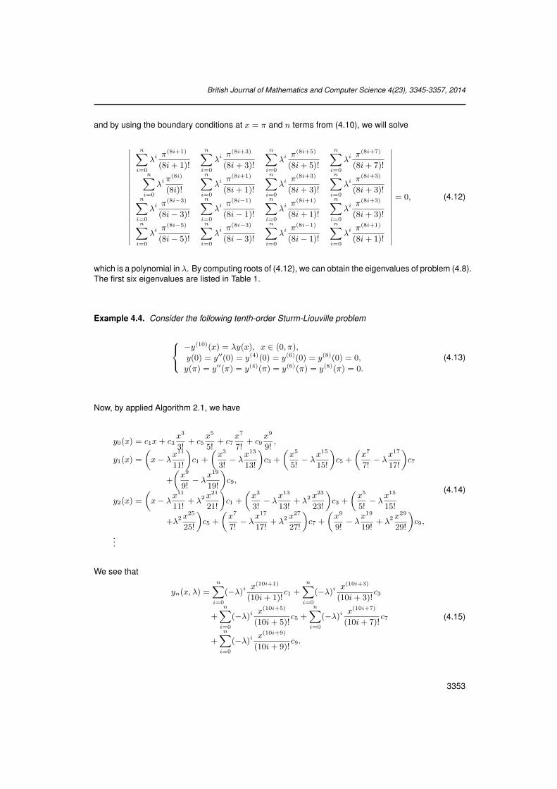
Example 4.4. Consider the following tenth-order Sturm-Liouville problem

−y(10)(x) = λy(x), x ∈ (0, π),

y(0) = y′′(0) = y(4)(0) = y(6)(0) = y(8)(0) = 0,

y(π) = y′′(π) = y(4)(π) = y(6)(π) = y(8)(π) = 0.

(4.13)

Now, by applied Algorithm 2.1, we have

y0(x) = c1x+ c3x3

3!+ c5

x5

5!+ c7

x7

7!+ c9

x9

9!,

y1(x) =

(x− λx

11

11!

)c1 +

(x3

3!− λx

13

13!

)c3 +

(x5

5!− λx

15

15!

)c5 +

(x7

7!− λx

17

17!

)c7

+

(x9

9!− λx

19

19!

)c9,

y2(x) =

(x− λx

11

11!+ λ2 x

21

21!

)c1 +

(x3

3!− λx

13

13!+ λ2 x

23

23!

)c3 +

(x5

5!− λx

15

15!

+λ2 x25

25!

)c5 +

(x7

7!− λx

17

17!+ λ2 x

27

27!

)c7 +

(x9

9!− λx

19

19!+ λ2 x

29

29!

)c9,

...

(4.14)

We see that

yn(x, λ) =

n∑i=0

(−λ)i x(10i+1)

(10i+ 1)!c1 +

n∑i=0

(−λ)i x(10i+3)

(10i+ 3)!c3

+

n∑i=0

(−λ)i x(10i+5)

(10i+ 5)!c5 +

n∑i=0

(−λ)i x(10i+7)

(10i+ 7)!c7

+

n∑i=0

(−λ)i x(10i+9)

(10i+ 9)!c9.

(4.15)

3353


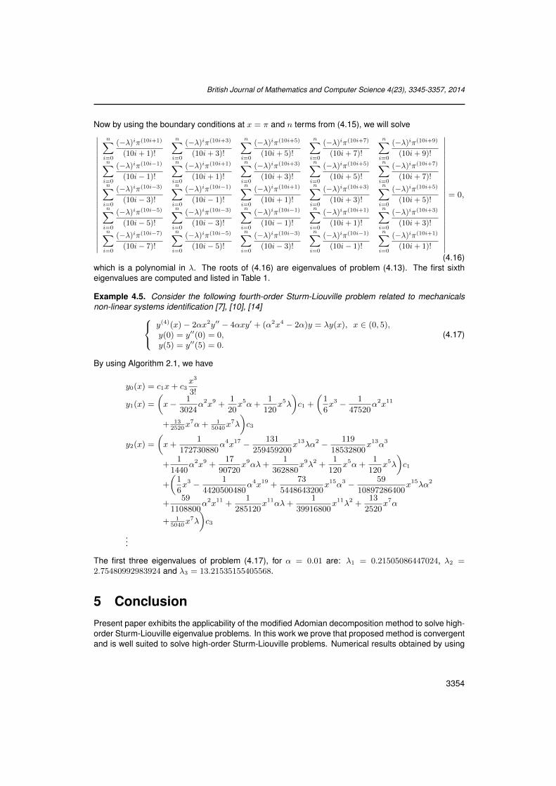
Now by using the boundary conditions at x = π and n terms from (4.15), we will solve∣∣∣∣∣∣∣∣∣∣∣∣∣∣∣∣∣∣∣∣∣∣∣

n∑i=0

(−λ)iπ(10i+1)

(10i+ 1)!

n∑i=0

(−λ)iπ(10i+3)

(10i+ 3)!

n∑i=0

(−λ)iπ(10i+5)

(10i+ 5)!

n∑i=0

(−λ)iπ(10i+7)

(10i+ 7)!

n∑i=0

(−λ)iπ(10i+9)

(10i+ 9)!n∑

i=0

(−λ)iπ(10i−1)

(10i− 1)!

n∑i=0

(−λ)iπ(10i+1)

(10i+ 1)!

n∑i=0

(−λ)iπ(10i+3)

(10i+ 3)!

n∑i=0

(−λ)iπ(10i+5)

(10i+ 5)!

n∑i=0

(−λ)iπ(10i+7)

(10i+ 7)!n∑

i=0

(−λ)iπ(10i−3)

(10i− 3)!

n∑i=0

(−λ)iπ(10i−1)

(10i− 1)!

n∑i=0

(−λ)iπ(10i+1)

(10i+ 1)!

n∑i=0

(−λ)iπ(10i+3)

(10i+ 3)!

n∑i=0

(−λ)iπ(10i+5)

(10i+ 5)!n∑

i=0

(−λ)iπ(10i−5)

(10i− 5)!

n∑i=0

(−λ)iπ(10i−3)

(10i− 3)!

n∑i=0

(−λ)iπ(10i−1)

(10i− 1)!

n∑i=0

(−λ)iπ(10i+1)

(10i+ 1)!

n∑i=0

(−λ)iπ(10i+3)

(10i+ 3)!n∑

i=0

(−λ)iπ(10i−7)

(10i− 7)!

n∑i=0

(−λ)iπ(10i−5)

(10i− 5)!

n∑i=0

(−λ)iπ(10i−3)

(10i− 3)!

n∑i=0

(−λ)iπ(10i−1)

(10i− 1)!

n∑i=0

(−λ)iπ(10i+1)

(10i+ 1)!

∣∣∣∣∣∣∣∣∣∣∣∣∣∣∣∣∣∣∣∣∣∣∣

= 0,

(4.16)which is a polynomial in λ. The roots of (4.16) are eigenvalues of problem (4.13). The first sixtheigenvalues are computed and listed in Table 1.

Example 4.5. Consider the following fourth-order Sturm-Liouville problem related to mechanicalsnon-linear systems identification [7], [10], [14] y(4)(x)− 2αx2y′′ − 4αxy′ + (α2x4 − 2α)y = λy(x), x ∈ (0, 5),

y(0) = y′′(0) = 0,y(5) = y′′(5) = 0.

(4.17)

By using Algorithm 2.1, we have

y0(x) = c1x+ c3x3

3!

y1(x) =

(x− 1

3024α2x9 +

1

20x5α+

1

120x5λ

)c1 +

(1

6x3 − 1

47520α2x11

+ 132520

x7α+ 15040

x7λ

)c3

y2(x) =

(x+

1

172730880α4x17 − 131

259459200x13λα2 − 119

18532800x13α3

+1

1440α2x9 +

17

90720x9αλ+

1

362880x9λ2 +

1

120x5α+

1

120x5λ

)c1

+

(1

6x3 − 1

4420500480α4x19 +

73

5448643200x15α3 − 59

10897286400x15λα2

+59

1108800α2x11 +

1

285120x11αλ+

1

39916800x11λ2 +

13

2520x7α

+ 15040

x7λ

)c3

...

The first three eigenvalues of problem (4.17), for α = 0.01 are: λ1 = 0.21505086447024, λ2 =2.75480992983924 and λ3 = 13.21535155405568.

5 ConclusionPresent paper exhibits the applicability of the modified Adomian decomposition method to solve high-order Sturm-Liouville eigenvalue problems. In this work we prove that proposed method is convergentand is well suited to solve high-order Sturm-Liouville problems. Numerical results obtained by using

3354


the modified Adomian decomposition method described in Section 2 show excellent agreement withthe exact solution when one uses only a few terms.

Competing InterestsThe authors declare that no competing interests exist.

References[1] Greenberg L, Marletta M. Numerical methods for higher order Sturm-Liouville problems. J.

Comput. Appl. Math. 2000;125:367-383.

[2] Taher AHS, Malek A. An efficient algorithm for solving high-order Sturm-Liouville problems usingvariational iteration method. Fixed Point Theory. 2013;14:193-210.

[3] Pryce JD. Numerical Solution of Sturm-Liouville Problems. Oxford University Press, New York;1993.

[4] Zettl A. Sturm-Liouville Theory. American Mathematical Society, Providence, RI; 2005.

[5] Ledoux V, Daele MV. Solution of Sturm-Liouville problems using modified Neumann schemes.SIAM J. Sci. Comput. 2010;32:564-584.

[6] Greenberg L, Marletta M. Oscillation theory and numerical solution of fourth order Sturm-Liouvilleproblems. IAM J. Numer. Anal. 1995;15:319-356.

[7] Taher AHS, Malek A, Momeni-Masuleh SH. Chebyshev differentiation matrices for efficientcomputation of the eigenvalues of fourth-order Sturm-Liouville problems. Appl. Math. Mode.2013;37:4634-4642.

[8] Civalek Q, Ulker M. Free vibration analysis of elastic beams using harmonic differential quadrature(HDQ). Math. Comp. Appl. 2004;9:257-264.

[9] Greenberg L, Marletta M. Oscillation theory and numerical solution of sixth order Sturm-Liouvilleproblems. SIAM J. Numer. Anal. 1998;35:2070-2098.

[10] Taher AHS, Malek A. A new algorithm for solving sixth-order Sturm-Liouville problems. Inter. J.Appl. Math. 2011;24:631-639.

[11] Chandrasekhar S. On characteristic value problems in high order differential equations whicharise in studies on hydrodynamic and hydromagnetic stability. Amer. Math. Monthly. 1955;61:32-45.

[12] Chandrasekhar S. Hydrodynamic and Hydromagnetic Stability. Oxford: Clarenden Press; 1961.reprinted by Dover Books, New York; 1981.

[13] Attili BS. The Adomian decomposition method for computing eigenelements of Sturm-Liouvilletwo point boundary value problems. Appl. Math. Comput. 2005;168:1306-1316.

[14] Attili BS, Lesnic D. An efficient method for computing eigenelements of Sturm-Liouville fourth-order boundary value problems. Appl. Math. Comput. 2006;182:1247-1254.

[15] Lesnis D, Attili BS. An Efficient Method for Sixth-order Sturm-Liouville Problems. Int. J. Sci.Techn. 2007;2:109-114.

[16] Adomian G. A review of the decomposition method in applied mathematics. J. Math. Anal. Appl.1988;135:501-544.

[17] Adomian G, Rach R. Generalization of Adomian polynomials to functions of several variables.Comput. Math. Appl. 1992;24:11-24.

3355


[18] Adomian G. Solving Frontier Problems of Physics: the Decomposition Method. Boston, Kluwer;1994.

[19] Wazwaz AM. Approximate solutions to boundary value problems of higher order by the modifieddecomposition method. Comput. Math. Appl. 2000;40:679-691.

[20] Az-Zo’bi EA, Al-Khaled K. A new convergence proof of the Adomian decomposition method for amixed hyperbolic elliptic system of conservation laws. Appl. Math. Comput. 2010;217:4248-4256.

[21] Bougoffa L, Rach R, El Manouni S. A convergence analysis of the Adomian decompositionmethod for an abstract Cauchy problem of a system of first-order nonlinear differential equations.Int. J. Comput. Math. 2013;90:360-375.

[22] El-Sayed AMA, El-Kalla IL, Ziada EAA. Analytical and numerical solutions of multi-term nonlinearfractional orders differential equations. Appl. Numer. Math. 2010;60:788-797.

[23] El-Kalla IL. Convergence of Adomians method applied to a class of Volterra type integro-differential equations. Int. J. Differ. Equ. Appl. 2005;10:225-234.

[24] El-Kalla IL. Error estimate of the series solution to a class of nonlinear fractional differentialequations. Commun. Nonlinear Sci. Numer. Simulat. 2011;16:1408-1413.

[25] Hosseini MM, Nasabzadeh H. On the convergence of Adomian decomposition method. Appl.Math. Comput. 2006;182:536-543.

[26] Atkinson K, Han W. Theoretical Numerical Analysis: a Functional Analysis Framework.Monographs on Technical Aspects Vol. II, Dover, New York; 1988.

—————————————————————————————————————————————-c©2014 Taher et al.; This is an Open Access article distributed under the terms of the Creative Commons

Attribution License http://creativecommons.org/licenses/by/3.0, which permits unrestricted use, distribution, andreproduction in any medium, provided the original work is properly cited.

Peer-review history:The peer review history for this paper can be accessed here (Please copy paste the total link in yourbrowser address bar)www.sciencedomain.org/review-history.php?iid=669&id=6&aid=6299

3356

http://creativecommons.org/licenses/by/3.0


Table1:

Thefirstsix

eigenvaluesforE

xamples

1,3,4.

Ex.

kλ1

λ2

λ3

λ4

λ5

λ6

21.000012982591777

56.2788900298348613

0.99999999966975964.019803409965889

532.1493838773596314

1.00000000000000263.999993955805054

731.3614407118920192356.075545405737775

51.000000000000000

64.000000000480616728.997819007874182

4228.0494640868815361

61.000000000000000

63.999999999999987729.000000676691570

4095.8036027729234997

1.00000000000000064.000000000000000

728.9999999999170614096.000137789611629

81.000000000000000

64.000000000000000729.000000000000005

4095.99999995688488015625.010847562816665

46394.7835588779246459

1.00000000000000064.000000000000000

729.0000000000000004096.000000000006639

15624.99999355694682446656.493105853629153

101.000000000000000

64.000000000000000729.000000000000000

4095.99999999999999915625.000000002026883

46655.99953234411829911

1.00000000000000064.000000000000000

729.0000000000000004096.000000000000000

15625.00000000000000046655.999999999921245

121.000000000000000

64.000000000000000729.000000000000000

4096.00000000000000015625.000000000000000

46656.00000000000001513

1.00000000000000064.000000000000000

729.0000000000000004096.000000000000000

15625.00000000000000046656.000000000000000

21.0000000139424631

255.19124845165229343

1.0000000000000015255.9999758252043787

6582.15561267157610964

1.0000000000000000255.9999999999357797

6561.001487230086340065301.5245144208390651

51.0000000000000000

256.00000000000000006561.0000000165164423

65535.9727164431913067392431.0850276472580053

61.0000000000000000

256.00000000000000006561.0000000000000410

65535.9999993102692247390625.2710159350685007

1670123.85691559029983183

71.0000000000000000

256.00000000000000006561.0000000000000000

65535.9999999999950702390625.0000117142127737

1679614.13569369727015438

1.0000000000000000256.0000000000000000

6561.000000000000000065536.0000000000000000

390625.00000000016984101679615.9998824062972465

91.0000000000000000

256.00000000000000006561.0000000000000000

65536.0000000000000000390625.0000000000000009

1679615.999999997165399810

1.0000000000000000256.0000000000000000

6561.000000000000000065536.0000000000000000

390625.00000000000000001679615.9999999999999710

111.0000000000000000

256.00000000000000006561.0000000000000000

65536.0000000000000000390625.0000000000000000

1679616.000000000000000012

1.0000000000000000256.0000000000000000

6561.000000000000000065536.0000000000000000

390625.00000000000000001679616.0000000000000000

10.9997297302962838

21.0000000000064805

1023.97472654528975123

1.00000000000000001024.0000000076896544

59048.82339315853982574

1.00000000000000001023.9999999999999999

59049.00000014864836211048575.5634512260551001

51.0000000000000000

1024.000000000000000059048.9999999999999880

1048576.00000063736400299765624.3859898835405941

46

1.00000000000000001024.0000000000000000

59049.00000000000000001048575.9999999999998610

9765625.000001266577916960466175.3942395260829979

71.0000000000000000

1024.000000000000000059049.0000000000000000

1048576.00000000000000009765624.9999999999994714

60466176.00000158401526228

1.00000000000000001024.0000000000000000

59049.00000000000000001048576.0000000000000000

9765625.000000000000000060466175.9999999999989557

91.0000000000000000

1024.000000000000000059049.0000000000000000

1048576.00000000000000009765625.0000000000000000

60466176.000000000000000010

1.00000000000000001024.0000000000000000

59049.00000000000000001048576.0000000000000000

9765625.000000000000000060466176.0000000000000000

3357

Documents

Semi-analytical Approximation for Solving High-order … · Semi-analytical Approximation for Solving High-order ... where lim k!1 k = 1and each ... both in classical mechanics and