Comparison of the analytical approximation formulaand Newton’s method for solving a class of nonlinear

Black-Scholes parabolic equations ∗

Karol Duris1, Shih-Hau Tan2, Choi-Hong Lai3, and Daniel Sevcovic4

1National Bank of Slovakia, Slovakia, e-mail: duris.karol@gmail.com2Department of Mathematical Sciences, University of Greenwich, London, UK, e-mail:

s.tan@gre.ac.uk3Department of Mathematical Sciences, University of Greenwich, London, UK, e-mail:

C.H.Lai@greenwich.ac.uk4Department of Applied Mathematics and Statistics, Division of Applied Mathematics,

Comenius University, Bratislava, Slovakia, e-mail: sevcovic@fmph.uniba.sk

Abstract

Market illiquidity, feedback effects, presence of transaction costs, risk from un-protected portfolio and other nonlinear effects in PDE based option pricing modelscan be described by solutions to the generalized Black-Scholes parabolic equationwith a diffusion term nonlinearly depending on the option price itself. Different lin-earization techniques such as Newton’s method and analytic asymptotic approxima-tion formula are adopted and compared for a wide class of nonlinear Black-Scholesequations including, in particular, the market illiquidity model and the risk-adjustedpricing model. Accuracy and time complexity of both numerical methods are com-pared. Furthermore, market quotes data was used to calibrate model parameters.

Keywords: Nonlinear PDE, Asymptotic Formula, Newton’s Method, Finite Dif-ference Method, Option Pricing, Black-Scholes Equation

MSC 2010 Classification: 35C20, 35K55, 91G60

1 Introduction

According to the classical theory due to Black, Scholes and Merton an option in astylized and idealized financial market can be priced by a solution V = V (S, t) tothe linear Black–Scholes parabolic equation:

∂V

∂t+

1

2σ2S2∂

2V

∂S2+ (r − q)S∂V

∂S− rV = 0, (1)

∗The final publication is available at www.degruyter.com once it is published

1

arX

iv:1

511.

0566

1v2

[q-

fin.

PR]

24

Nov

201

5

where r > 0 is the interest rate of a zero-coupon bond, q ≥ 0 is the dividend yieldrate and σ > 0 is a constant historical volatility of the underlying asset price process{St, t ≥ 0}, which is assumed to follow a stochastic differential equation

dSt = (r − q)Stdt+ σStdWt, (2)

of the geometric Brownian motion with a drift r − q (cf. [22, 18, 25]). The linearBlack–Scholes equation with a constant volatility σ has been derived under severalrestrictive assumptions, for example, zero transaction costs, perfectly replicatedportfolio, frictionless, market completeness, etc.

In this paper, the main goal is to investigate and compare two numerical ap-proximation methods for solving a class of nonlinear generalizations of the linearBlack-Scholes equation (1) in which the volatility is assumed to be a function ofthe underlying asset price S and Gamma of the option (the Greek Gamma is thesecond derivative ∂2SV ), i.e.

σ = σ(∂2SV, S) . (3)

The motivation for solving the nonlinear Black–Scholes equation (1) with the volatil-ity function σ of the form (3) arises from more realistic option pricing models inwhich one can take into account nontrivial transaction costs, market feedbacks, riskfrom unprotected portfolio and other effects. In the last decades, some of the re-strictive assumption of the classical Black–Scholes theory [4] have been relaxed inorder to model, for instance, presence of constant transaction costs (see e.g. Leland[23], Hoggard et al. [16]), non-constant transaction costs (see e.g. Amster et al.[1], Sevcovic and Zitnanska [26]), uncertain volatility model (cf. Avellaneda andParas [2]), feedback and illiquid market effects due to large traders choosing givenstock-trading strategies (cf. Frey [12], Frey and Patie [13], Frey and Stremme [14],Schonbucher and Wilmott [24]), imperfect replication and investor’s preferences (cf.Barles and Soner [3]), risk from an unprotected portfolio (cf. Kratka [21], Jandackaand Sevcovic [19]). Efficient techniques and fast computational methods for pricingderivative securities is a practical task in financial quotes markets. Therefore, real-istic PDE based option models including, in particular, nonlinear generalizations ofthe Black–Scholes equation have to be solved in a fast and efficient way. However,in most important cases there is no explicit formula except for some special caseswith non-standard pay-off diagrams (cf. Bordag [6]). This is the reason why nu-merical methods for solving nonlinear Black–Scholes equation have to be developedand analyzed.

In this paper, attention is focused on a class of nonlinear Black-Scholes equations.In particular, the nonlinear volatility model developed by Frey et al. [12, 11, 13,14] and the risk-adjusted pricing methodology model proposed and investigated byKratka [21] and Jandacka and Sevcovic [19, 25] are the main concern of this work.In a series of papers [12, 11, 13, 14] Frey et al. considered a model in which theprice of an underlying asset is affected by specific hedging strategies due to a largetrader. Supposing that a large trader uses a given stock-holding strategy αt andthe underlying stock price process satisfies the following SDE:

dSt = µStdt+ σStdWt + ρStdαt, (4)

where µ is a drift parameter, σ > 0 is the volatility of the process and 0 ≤ ρ < ρis the so-called market liquidity parameter. It is worth noting that the quantity

2

1/(ρSt) measures the size of the change in the stock-holding position of the largetrader. Notice that if αt ≡ 0 or ρ = 0, the stock price St follows the geometricBrownian motion. In [12] Frey (see also [13, 14]) showed that the option price isthen a solution to a nonlinear volatility Black-Scholes equation of the form:

∂V

∂t+

1

2σ(∂2SV, S)2S2∂

2V

∂S2+ (r − q)S∂V

∂S− rV = 0, (5)

for 0 ≤ S <∞ and 0 ≤ t < T where T is the maturity time. The nonlinear volatilityfunction σ is given by

σ(∂2SV, S) = σ(1− ρS∂2SV )−1, (6)

where σ is a constant historical volatility. A solution V = V (S, t) is subject to theterminal pay-off condition describing call or put option with expiration price E > 0,i.e.

V (S, T ) = (S − E)+ (call option), V (S, T ) = (E − S)+ (put option). (7)

Another nonlinear model was proposed by Kratka [21]. It was further general-ized and analyzed by Jandacka and Sevcovic in [19, 25]. The model is constructedfollowing the classical Leland approach for modeling transaction costs (cf. [23])in which the time between consecutive portfolio rearrangements is subject to op-timization with respect to the risk arising from an unprotected portfolio. In thisrisk-adjusted pricing methodology (RAPM) model the nonlinear volatility functionhas the form:

σ(∂2SV, S)2 = σ2(1 + µ(S∂2SV )13 ). (8)

Construction of explicit solutions to equation (5) with the nonlinear volatilityfunction as the one defined in (8) were recently provided by Bordag and Frey [5] (seealso [6]). Several invariant solutions were constructed by means of the invariant Liegroup theory. These invariant solutions depend on various parameters restrictingthe class of solutions. In particular, not every pay-off diagram can be considered. Ingeneral, there is no exact pricing formula for the case of a call or put terminal pay-offs. Hence efficient numerical techniques for solving such nonlinear Black–Scholesequations are required.

A numerical method proposed and investigated by Jandacka and Sevcovic [19] isbased on the transformation H = S∂2SV, x = ln(S/E), τ = T − t, which transformsequation (5) with σ = σ(S∂2SV ) into a porous media type of quasilinear parabolicequation:

∂H

∂τ=

∂2

∂x2β(H) +

∂

∂xβ(H) + (r − q)∂H

∂x− qH , (9)

where β(H) = 12σ

2(H)H is an increasing function. For instance, in the case of the

volatility function given by (6) one obtains β(H) = σ2

2 H (1− ρH)−2 for H < Hmax

(see [25] for details). In the recent paper [26], Sevcovic and Zitnanska investigatedthe nonlinear equation (9) in the context of modeling variable transaction costs.The existence of classical Holder smooth solutions was proved and useful boundsfor the solution were derived.

The transformation technique developed in [19] allows for construction of a semi-implicit finite volume based numerical scheme for solving (9). There are otherapproaches dealing mainly with the nonlinear equation (5) for the option price rather

3

than for its transformation H = S∂2SV . Another method using quasilinearizationtechnique for solving the fully nonlinear parabolic equation (5) was proposed andanalyzed by Koleva and Vulkov [20]. A consistent monotone explicit finite differencenumerical scheme was analyzed by Company et al. in the context of the Frey andPatie model (5) with a nonlinear volatility function given by (6). In [10] Ehrhardtand Valkov derived an unconditionally stable explicit numerical scheme for solvingthe same problem and provided necessary numerical analysis of the scheme.

In this paper, two numerical approximation methods based on the asymptoticperturbation analysis and the Newton linearization technique are developed. Thesemethods are used to solve a wide class of nonlinear Black-Scholes equations. Thefirst method is the asymptotic perturbation method which is based on asymptoticexpansion of the solution into power series in a small model parameter. The firstorder expansion then corresponds to an explicit analytic approximation formularequiring only one-dimensional numerical integration which can be computed in afast and efficient way. The second method is based on Newton’s iterative method forsolving the corresponding nonlinear problem in each temporal discretization level.It is applicable to a rather general nonlinear case not restricted by any specifictypes of equations and boundary and terminal conditions. In [15] Heider usedNewton’s iterative method for solving equation (5) with four types of nonlinearvolatilities and different finite different schemes. Note that different variants ofNewton’s linearization and their implementation are also discussed and comparedin this paper.

The paper is organized as follows. In section 2 an explicit analytic approximationformula for solving a general class of nonlinear volatility models is derived. In section3 an algorithm utilizing Newton’s method for solving equation (5) is described andanalyzed. Several comparisons of both methods are discussed in section 4. Examplesof solution to the Frey and Patie model and RAPM model are presented. Finally,section 5 contains an example of model calibration to real market quotes data.

2 Analytic approximation formula based asymp-

totic perturbation analysis

In this section, an analytic approximation formula for pricing European call or putoptions with a nonlinear volatility is derived. Typically this paper considers a wideclass of nonlinear volatility functions taking the following form:

σ(∂2SV, S, T − t)2 = σ2 + 2εA(T − t)Sγ−1Hδ−1, where H = S∂2V

∂S2.

The powers γ, δ, the parameter ε as well as the function A(T−t) depend on the cho-sen nonlinear volatility model. For example, in the case of the Frey and Patie modelwith the nonlinear volatility function given by (6), σ(∂2SV, S) = σ/(1 − ρS∂2SV ) ≈σ(1 + ρS∂2SV ) and the parameters are

ε = ρ, γ = 1, δ = 2, A(T − t) = σ2,

and the small model parameter ε can be identified with 0 < ρ� 1.

4

For the RAPM model with the nonlinear volatility function given by (8) theparameters can be identified as follows:

ε = µ, γ = 1, δ = 4/3, A(T − t) = σ2/2,

and the small parameter ε is identified with 0 < µ� 1.Equation (5) can now be rewritten as

L(V, ε) ≡ ∂V

∂t+

1

2σ(∂2SV, S)2S2∂

2V

∂S2+ (r − q)S∂V

∂S− rV = 0,

V (S, T ) = V (S),

(10)

where V is the prescribed pay-off diagram. The problem is to seek the option pricein the form of an asymptotic expansion in terms of a small parameter (cf. [17]).More precisely,

V = V0 +

N∑i=1

εiVi +O(εN+1), (11)

where the leading term V0 ≡ VBS is simply a solution to the linear Black-Scholesmodel.

The aim here is to derive an asymptotic approximation formula obtained fromthe first two terms in the asymptotic expansion, i.e.

V (S, t) ≈ V0(S, t) + εV1(S, t). (12)

In order to obtain an explicit formula for the second term V1 in the expansion,equation (10) is first approximated as follows:

L(V, ε) ≈ L0(V ) + εL1(V ) ≈ L0(V0 + εV1) + εL1 (V0 + εV1) , (13)

where L0 is a linear and L1 is a nonlinear differential operator in V ,

L0(V ) ≡ ∂V

∂t+

1

2σ2S2∂

2V

∂S2+ (r − q)S∂V

∂S− rV,

L1(V ) ≡ A(T − t)Sγ(S∂2V

∂S2

)δ.

Hence the first order approximation of the equation L(V, ε) = 0 reads as follows:

L0(V0) + ε(L0(V1) + L1(V0)) = 0 (14)

satisfying the initial condition:

V (S, T ) ≡ V0(S, T ) + εV1(S, T ) = V (S). (15)

Equation (14) with the initial condition (15) can be separated into a system ofequations in powers of ε, i.e.

O(ε0) : L0(V0) = 0,

V0(S, T ) = (S − E)+ (call), V0(S, T ) = (E − S)+ (put)

O(ε) : L0(V1) = −L1(V0),V1(S, T ) = 0.

5

The solution V0 can be obtained by solving the linear Black-Scholes equation. Thesecond equation for V1 is a non-homogeneous PDE with zero initial condition.

Introduce H0 = S ∂2V0∂S2 , the equation L0(V1) = −L1(V0) can be rewritten as

follows {L0(V1) = −A(T − t)SγHδ

0 , (S, t) ∈ (0,∞)× [0, T ),V1(S, T ) = 0, S ∈ (0,∞).

(16)

Therefore, equation (16) can be solved once the value of V0(S, t) is evaluated toobtain H0. Recall

V0(S, t) = Se−q(T−t)Φ(d1)− Ee−r(T−t)Φ(d2),

d1,2 =ln S

E +(r − q ± σ2

2

)(T − t)

σ√T − t

,

where Φ(d) = 1√2π

∫ d−∞ e

−x2/2dx is the cumulative distribution function of the stan-

dard normal distribution. Hence

H0 = S∂2V0∂S2

=e−qτΦ′(d1)

σ√τ

.

In order to solve equation (16) one adopts the usual transformation (see e.g.[25])

τ = T − t, S = Eex, eαx+βτu(x, τ) = V1(S, t), (17)

where

α =1

2+q − rσ2

, β = −

(σ2

8+r + q

2+

(r − q)2

2σ2

)= − σ

2

2α2 − r. (18)

Equation (16) is thus transformed to as follows:

−eαx+βτ ∂u∂τ

+ eαx+βτσ2

2

∂2u

∂x2= −A(τ) Eγeγx e−qδτ

(Φ′(d1)

)δσδτ

δ2

,

u(x, 0) = 0.

(19)

The term d1 corresponds to d1 after transformation (17). It is given by

d1 =x

σ√τ

+

(r − q + σ2

2

)σ

√τ =

x

σ√τ

+ (1− α)σ√τ .

Finally, equation (19) can be simplified to as the equation below

∂u

∂τ− σ2

2

∂2u

∂x2=

EγA(τ)(2πσ2τ

) δ2

e−δ

2σ2τx2+[γ−δ−α(1−δ)]x−[β+qδ+ δ

2(1−α)2σ2]τ ,

u(x, 0) = 0, (x, τ) ∈ R× [0, T ]. (20)

6

Theorem 2.1. Let u(x, τ) be a solution to (20) satisfying the growth condition|u(x, τ)| ≤ Meb|x|

2for all x ∈ R, τ ∈ [0, T ] where M, b are some constants. Then

u(x, τ) is given by the formula:

u(x, τ) = Eγ∫ τ

0

A(ξ)

Λ(τ, ξ)e

[P2σ2

2(δ−1)+β(δ−1)

]ξ+ Px

1−δ+P2σ2τ2(1−δ)2

−[δx2

2σ2+Pxδτ

1−δ +P2σ2δτ2

2(1−δ)2

]1

Q(τ,ξ)dξ,

(21)where P = γ − δ − α(1 − δ) is a constant depending on the model parameters andthe functions Q(τ, ξ) and Λ(τ, ξ) are defined as follows:

Q(τ, ξ) = δτ + (1− δ)ξ, Λ(τ, ξ) = (2πσ2)δ2 ξ

δ−12

√Q(τ, ξ). (22)

The proof of this theorem is a straightforward application of the variation ofconstants formula and can be found in the Appendix. As a consequence of theprevious theorem an explicit expression for the first order approximation of theoption price can be obtained. Taking V1(S, t) = eαx+βτu(x, τ) leads to

V1(S, t) =Eγ

(2πσ2)δ2

(S

E

) γ−δ1−δ

e

{β+

[γ−δ−α(1−δ)]2σ2

2(1−δ)2

}(T−t)

(23)

×∫ T−t

0

A(ξ)

ξδ−12

√δ(T − t) + (1− δ)ξ

eKξ−M(S) 1

δ(T−t)+(1−δ)ξ dξ,

where K is a constant given by

K =

[γ − δ − α(1− δ)

]2σ2

2(δ − 1)+ β(δ − 1)

and

M(S) =δ

2σ2

(lnS

E

)2

+

[γ − δ − α(1− δ)

]δ(T − t)

1− δlnS

E

+

[γ − δ − α(1− δ)

]2σ2δ(T − t)2

2(1− δ)2.

The analytic approximation of the option price V (S, t) can then be evaluated byusing equation (12).

3 Implicit finite difference scheme using New-

ton’s method

A standard way of solving equation (5) numerically is to use implicit temporal dis-cretization in combination with a finite difference method for approximating thederivatives. Note the volatility term appearing in (6) and (8) is nonlinear and ateach time level an iterative technique is to be applied. The method of frozen coef-ficient technique is commonly applied to handle the nonlinearity though sometimesit converges slowly without proper initial guess. To obtain a better convergence

7

rate, Newton’s method has to be employed in combination with a temporal implicitdiscretization scheme.

Newton’s method is a linearization technique with many variants and each takesdifferent implementation. In this section two approaches are discussed. The firstapproach (denoted by NM1) addresses the root-finding problem of the nonlinearsystem derived from an implicit scheme in which calculation of the Jacobian matrixis used to update the approximate solution. The second approach (NM2) linearizesthe original equation in which a correction term is to be solved and used to updatethe approximate solution.

3.1 Newton’s Method (NM1)

Using standard finite difference notations and the transformation τ = T − t animplicit finite difference scheme which replaces equation (5) reads as follows:

V n+1i − V n

i

∆τ− 1

2σn+1i S2

i

V n+1i+1 − 2V n+1

i + V n+1i−1

(∆S)2− rSi

V n+1i+1 − V

n+1i−1

2∆S+ rV n+1

i = 0.

The volatility function σ as given by (6) may be discretised as

σn+1i = σ(1− ρSi

V n+1i+1 − 2V n+1

i + V n+1i−1

(∆S)2)−1.

Here Si = (i − 1)∆S, i = 1, · · · ,M , and n = 1, · · · , N − 1, where M and N arethe numbers of grid points for spatial and temporal discretization respectively. Theabove equation can be simplified as follows:

H(V n+1)V n+1 − V n = 0, (24)

where H(V n+1) is an M×M tridiagonal matrix whose elements nonlinearly dependon V n+1. Introducing the mapping

G(V n+1) = H(V n+1)V n+1 − V n, (25)

turns the original problem to the construction of a solution V n+1 of the equa-tion G(V n+1) = 0 at each time level. Newton’s method is applied to solve theroot-finding problem which requires the Jacobian matrix of the function G to becomputed. An initial guess chosen as the solution V from the previous time levelusually reduces the number of Newton’s iterations.

8

10 K. Ďuriš, S.-H. Tan, C.-H. Lai, D. Ševčovič

turns the original problem to the construction of a solution V n+1 of the equationG(V n+1) = 0 at each time level. Newton’s method is applied to solve the root-finding problem which requires the Jacobian matrix of the function G to becomputed. An initial guess chosen as the solution V from the previous timelevel usually reduces the number of Newton’s iterations.

Algorithm 1: Newton’s Method (NM1)Input: initial guess V n+1, tol, initial condition V 1 = V (S, τ = 0)Output: V N = V (S, τ = T )for n = 1 : N − 1 do

1. G(V n+1) = H(V n+1)V n+1 − V n ;2. if ‖G(V n+1)‖ < tol then

break;else

V n+1 = V n+1 −[Jac(G(V n+1))

]−1G(V n+1);

go back to 1.end

endend

In order to compute the Jacobian matrix efficiently, a decomposition of thematrix H(V n+1) may be adopted as below

H(V n+1) = Σn+1 H1 +H2, where Σn+1 = Diag((σn+1i )2).

Note that H1 and H2 are constant tridiagonal matrices. By using this decom-position, the Jacobian matrix of G becomes

Jac(G(V n+1)) = ∂[H(V n+1)V n+1]∂V n+1 = H(V n+1) + Diag(H1 V

n+1)∇(Σn+1) ,

where

∇(Σn+1) = ((∇(σn+11 )2)T , (∇(σn+1

2 )2)T , ..., (∇(σn+1M )2)T )T ,

here ∇(σn+1k )2 is treated as a row vector.

This decomposition simplifies the computing of the Jacobian matrix interms of the nonlinear volatility. Each gradient ∇(σn+1

k )2 can be obtained byeither deriving the analytic expression for σ or by using a finite difference ap-proximation of the spatial derivatives.

In order to compute the Jacobian matrix efficiently, a decomposition of thematrix H(V n+1) may be adopted as below

H(V n+1) = Σn+1H1 +H2, where Σn+1 = Diag((σn+1i )2).

Note that H1 and H2 are constant tridiagonal matrices. By using this decomposi-tion, the Jacobian matrix of G becomes

Jac(G(V n+1)) =∂[H(V n+1)V n+1]

∂V n+1= H(V n+1) + Diag(H1 V

n+1)∇(Σn+1) ,

where∇(Σn+1) = ((∇(σn+1

1 )2)T , (∇(σn+12 )2)T , ..., (∇(σn+1

M )2)T )T ,

here ∇(σn+1k )2 is treated as a row vector.

This decomposition simplifies the computing of the Jacobian matrix in terms ofthe nonlinear volatility. Each gradient ∇(σn+1

k )2 can be obtained by either derivingthe analytic expression for σ or by using a finite difference approximation of thespatial derivatives.

3.2 Waveform-Newton’s Method (NM2)

The second approach of applying Newton’s linearization is to consider a smoothfunction F representing the nonlinear Black-Scholes equation, i.e.

F (Vτ , VS , VSS , V ) ≡ Vτ −1

2σ2(VSS , S)S2VSS − rSVS + rV = 0.

Here Vτ , VS , VSS abbreviate the partial derivatives ∂τ , ∂SV, ∂2SV respectively. The

linearization of the function F at (V ∗τ , V∗S , V

∗SS , V

∗) in direction (vτ , vS , vSS , v) readsas follows:

F (V ∗τ + vτ , V∗S + vS , V

∗SS + vSS , V + v)

= F (V ∗τ , V∗S , V

∗SS , V

∗) +∂F

∂Vτvτ +

∂F

∂VSvS +

∂F

∂VSSvSS +

∂F

∂Vv +O(D2),

(26)

9

where D2 represents all higher order terms and the partial derivatives are evaluatedat (V ∗τ , V

∗S , V

∗SS , V

∗).

Equation (26) transforms equation (5) into a linear partial differential equation ofthe correction term v with zero boundary and initial conditions. This equation canbe solved easily because all coefficients of equation (26) are determined. Similar tothe first approach (NM1), these coefficients can be evaluated either by the analyticexpression for σ or by a finite difference approximation. Eventually, the problembecomes

∂F

∂V ∗τvn −∆τF (V ∗τ , V

∗S , V

∗SS , V

∗) = H∗(V ∗)vn+1. (27)

Again, an initial guess can be set to the solution from previous time level in thealgorithm.12 K. Ďuriš, S.-H. Tan, C.-H. Lai, D. Ševčovič

Algorithm 2: Waveform-Newton’s Method (NM2)Input: initial guess V ∗, tol, initial condition V 1 = V (S, τ = 0), v1 = 0Output: V N = V (S, τ = T )for n = 1 : N − 1 do

1. Calculate ∂F∂V ∗

τ, ∂F∂V ∗

S, ∂F∂V ∗

SS, ∂F∂V ∗ ;

2. Solve equation (27) to get vn+1 ;if ‖vn+1‖ < tol then

V n+1 = V ∗; break;else

V ∗ = V ∗ + vn+1 ;go back to 1.

endend

end

0 50 100 150 2002

4

6

8

10

12

14x 10

−6

number of grid points

Diff

eren

ce u

nder

l 2 nor

m

NM1 V.S NM2

0 50 100 150 2000.5

1

1.5

2

2.5

3x 10

−5

number of grid points

Diff

eren

ce u

nder

max

imum

nor

m

NM1 V.S NM2

Fig. 1. Difference of the solution between NM1 and NM2 with respect to the number ofgird points under the integral l2 norm (left) and maximum norm (right).

The main difference between algorithm NM1 and NM2 is the linearization errorO(D2). Figure 1 illustrates this error which can be reduced by refining the meshusing more grid points. Both approaches can approximate to the same value with∆S and ∆t small enough and can be easily applied to different nonlinear volatilitiesmodels as well as different types of options.

4 Numerical experiments

In this section a comparison is made of two different numerical approximation meth-ods for computing prices of European call options based on Newton’s methods(NM1, NM2) and the analytic asymptotic approximation formula developed in sec-tion 2. In the asymptotic approximation formula, the Frey and Patie model (6)and the RAPM model (8) are characterized by the following parameters: (ε, δ, γ) =(ρ, 2, 1) and (ε, δ, γ) = (µ, 4/3, 1), respectively. For the finite difference Newton’s

10

0 50 100 150 2002

4

6

8

10

12

14x 10

−6

number of grid points

Diff

eren

ce u

nder

l 2 nor

m

NM1 V.S NM2

0 50 100 150 2000.5

1

1.5

2

2.5

3x 10

−5

number of grid points

Diff

eren

ce u

nder

max

imum

nor

m

NM1 V.S NM2

Figure 1: Difference of the solution between NM1 and NM2 with respect to the numberof gird points under the integral l2 norm (left) and maximum norm (right).

methods (NM1, NM2) terminal and boundary conditions were chosen as:V (S, T ) = (S − E)+, for 0 ≤ S < Smax,V (0, t) = 0, for 0 ≤ t ≤ T,V (S, t) = S − Ee−r(T−t), when S = Smax.

Common model parameters were chosen as: σ = 0.4, E = 100, r = 0.03, q =0, Smin = 0, Smax = 300, T = 1/12 and a transformation τ = T − t was used.The tolerance for Newton’s iterations was set as tol = 10−8. The initial guess inNewton’s methods at the first time level was chosen as the constant value of 1. Inthe subsequent temporal levels the initial guess was taken from the approximatesolution at the previous time level. The fast and robust Thomas algorithm fortridiagonal solver was used in Newton’s method. Calculation of integrals for theasymptotic formula was done by using the built-in Matlab function integral.

4.1 Comparison of numerical methods with explicit in-variant solution

In order to ensure all the numerical solvers mentioned in section 3 are accurate, theexplicit invariant solutions for the Frey and Patie model derived by Bordag in [5,(86), (87)] with parameters c = −0.05, d1 = 0, d2 = 30 were computed and taken asreference solutions for evaluating experimental order of convergence. The boundaryconditions and initial conditions were generated from these invariant solutions.

The table containing the experimental order of convergence (or convergenceratio) is constructed from the convergence rate of the error defined as follows:

a =log((Err)m+1/(Err)m)

log((∆S)m+1/(∆S)m).

Here the error Err is defined as Err = ‖V (S, τ) − V (S, τ)‖/‖V (S, τ)‖ for S ∈[0.5E, 1.5E], where V (S, τ) is the solution from numerical solver, and V (S, τ) is from

11

Table 1: EOC for the Frey and Patie Model with the l∞ maximum norm

∆τ ∆S ErrNM1 aNM1 ErrNM2 aNM2 ErrFrozen aFrozen

0.00833 30 2.93e-05 — 2.93e-05 — 2.93e-050.00208 15 1.72e-06 4.09 1.72e-06 4.09 1.72e-06 4.095.21e-04 7.5 1.02e-07 4.08 1.02e-07 4.08 1.02e-07 4.081.30e-04 3.75 2.50e-08 2.02 2.50e-08 2.02 2.50e-08 2.023.26e-05 1.875 5.00e-09 2.32 5.00e-09 2.32 5.00e-09 2.328.14e-06 0.9375 1.25e-09 2.00 1.25e-09 2.00 1.25e-09 2.00

Table 2: EOC for the Frey and Patie Model with the l2 integral norm

∆τ ∆S ErrNM1 aNM1 ErrNM2 aNM2 ErrFrozen aFrozen

0.00833 30 2.93e-05 — 2.93e-05 — 2.93e-050.00208 15 1.79e-06 4.03 1.79e-06 4.03 1.79e-06 4.035.21e-04 7.5 1.39e-07 3.68 1.39e-07 3.68 1.39e-07 3.681.30e-04 3.75 4.46e-08 1.64 4.46e-08 1.64 4.46e-08 1.643.26e-05 1.875 1.25e-08 1.83 1.25e-08 1.83 1.25e-08 1.838.14e-06 0.9375 4.32e-09 1.53 4.32e-09 1.53 4.32e-09 1.53

the invariant solution. The ratio (∆S)2/∆τ is fixed to be 108000, and (∆S)m+1/(∆S)m =0.5. Tables 1 and 2 show results for the l∞ maximum norm and l2 integral norm.Both results demonstrate that all the solvers converge to the same solution whichconverges to the explicit invariant solution with refined grid points.

4.2 Comparison of accuracy of Newton’s method andasymptotic analytic formula

In Figure 2 errors between different methods were plotted in order to analyzethe changes of the numerical approximation with respect to different model pa-rameter ρ in the Frey and Patie model and µ in the RAPM model. The error‖V (S, τ)− V (S, τ)‖/‖V (S, τ)‖ for S ∈ [0.5E, 1.5E] was computed with the l∞ max-imum norm where V was calculated from Newton’s method and V was evaluatedby the asymptotic formula.

The difference between Newton’s method and the asymptotic formula can bereduced by taking smaller values of model parameters as shown in the Figure 2.When ρ and µ become larger, the difference increases. Notice that in the asymptoticformula, higher order terms such us O(ρ2) and O(µ2) are ignored. These terms cannot be neglected when considering larger values of the model parameters.

4.3 Time complexity comparison of Newton’s methodand analytic asymptotic formula

The comparison of time complexity is based on the implementation under the sameMatlab computing environment in order to ensure fair comparison. Since the CPUtime depends on the software implementation, the comparison is chosen to be based

12

0 0.002 0.004 0.006 0.008 0.010

0.5

1

1.5x 10

−3

ρ

Diff

eren

ce

NM1 V.S Asym

0 0.002 0.004 0.006 0.008 0.010

0.5

1

1.5x 10

−3

ρ

Diff

eren

ce

NM2 V.S Asym

0 0.002 0.004 0.006 0.008 0.010

0.5

1

1.5x 10

−3

µ

Diff

eren

ce

NM1 V.S Asym

0 0.002 0.004 0.006 0.008 0.010

0.5

1

1.5x 10

−3

µ

Diff

eren

ce

NM2 V.S Asym

Figure 2: Difference between the analytic asymptotic approximation formula and New-ton’s methods NM1(left), NM2(right) for the Frey and Patie model (top row) and theRAPM model (bottom row). The circled blue line corresponds to M = N = 50, the redline with stars corresponds to grid sizes M = N = 100, and the green line with diamondscorresponds to M = N = 200.

13

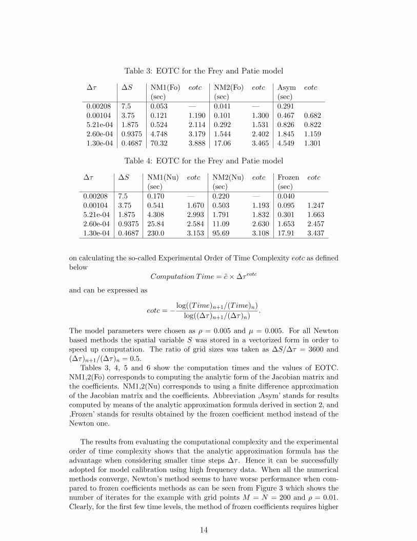
Table 3: EOTC for the Frey and Patie model

∆τ ∆S NM1(Fo) eotc NM2(Fo) eotc Asym eotc(sec) (sec) (sec)

0.00208 7.5 0.053 — 0.041 — 0.2910.00104 3.75 0.121 1.190 0.101 1.300 0.467 0.6825.21e-04 1.875 0.524 2.114 0.292 1.531 0.826 0.8222.60e-04 0.9375 4.748 3.179 1.544 2.402 1.845 1.1591.30e-04 0.4687 70.32 3.888 17.06 3.465 4.549 1.301

Table 4: EOTC for the Frey and Patie model

∆τ ∆S NM1(Nu) eotc NM2(Nu) eotc Frozen eotc(sec) (sec) (sec)

0.00208 7.5 0.170 — 0.220 — 0.0400.00104 3.75 0.541 1.670 0.503 1.193 0.095 1.2475.21e-04 1.875 4.308 2.993 1.791 1.832 0.301 1.6632.60e-04 0.9375 25.84 2.584 11.09 2.630 1.653 2.4571.30e-04 0.4687 230.0 3.153 95.69 3.108 17.91 3.437

on calculating the so-called Experimental Order of Time Complexity eotc as definedbelow

Computation T ime = c×∆τ eotc

and can be expressed as

eotc = − log((Time)n+1/(Time)n)

log((∆τ)n+1/(∆τ)n).

The model parameters were chosen as ρ = 0.005 and µ = 0.005. For all Newtonbased methods the spatial variable S was stored in a vectorized form in order tospeed up computation. The ratio of grid sizes was taken as ∆S/∆τ = 3600 and(∆τ)n+1/(∆τ)n = 0.5.

Tables 3, 4, 5 and 6 show the computation times and the values of EOTC.NM1,2(Fo) corresponds to computing the analytic form of the Jacobian matrix andthe coefficients. NM1,2(Nu) corresponds to using a finite difference approximationof the Jacobian matrix and the coefficients. Abbreviation ,Asym’ stands for resultscomputed by means of the analytic approximation formula derived in section 2, and,Frozen’ stands for results obtained by the frozen coefficient method instead of theNewton one.

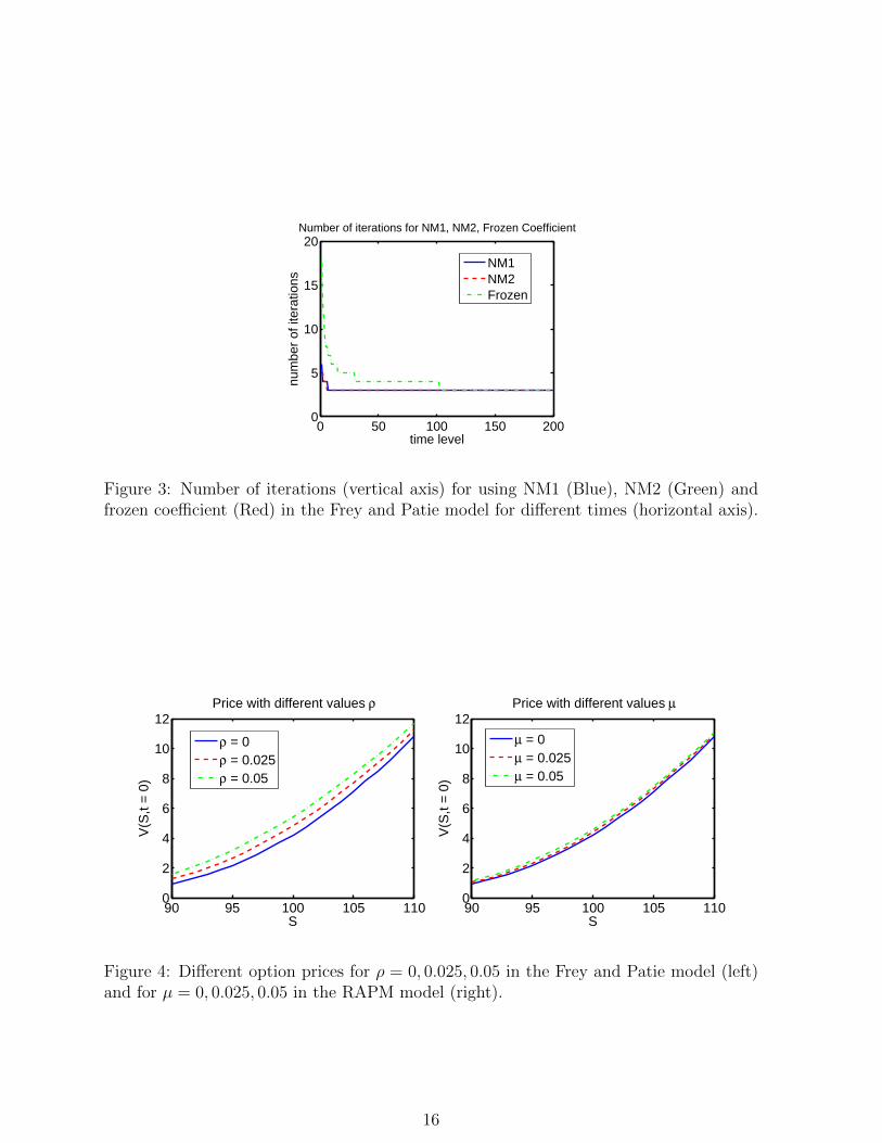
The results from evaluating the computational complexity and the experimentalorder of time complexity shows that the analytic approximation formula has theadvantage when considering smaller time steps ∆τ . Hence it can be successfullyadopted for model calibration using high frequency data. When all the numericalmethods converge, Newton’s method seems to have worse performance when com-pared to frozen coefficients methods as can be seen from Figure 3 which shows thenumber of iterates for the example with grid points M = N = 200 and ρ = 0.01.Clearly, for the first few time levels, the method of frozen coefficients requires higher

14

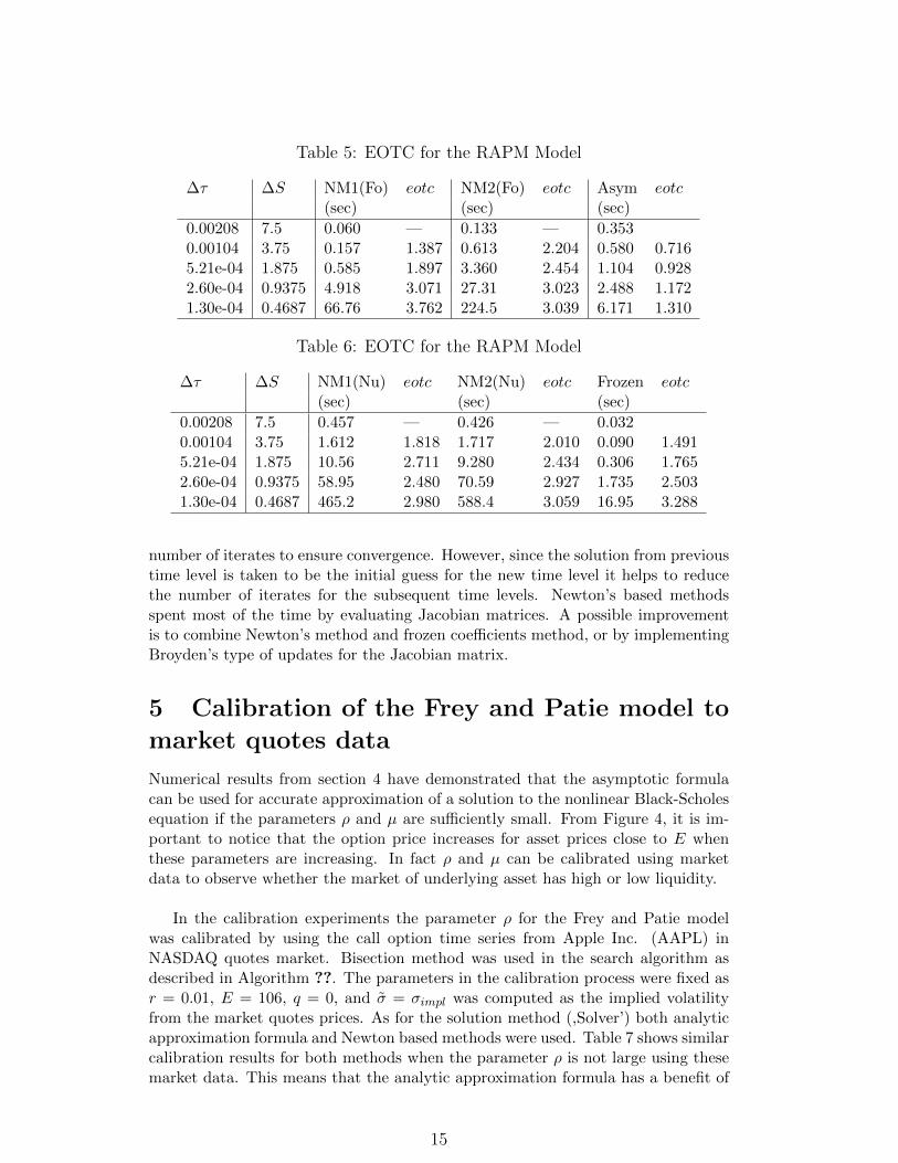
Table 5: EOTC for the RAPM Model

∆τ ∆S NM1(Fo) eotc NM2(Fo) eotc Asym eotc(sec) (sec) (sec)

0.00208 7.5 0.060 — 0.133 — 0.3530.00104 3.75 0.157 1.387 0.613 2.204 0.580 0.7165.21e-04 1.875 0.585 1.897 3.360 2.454 1.104 0.9282.60e-04 0.9375 4.918 3.071 27.31 3.023 2.488 1.1721.30e-04 0.4687 66.76 3.762 224.5 3.039 6.171 1.310

Table 6: EOTC for the RAPM Model

∆τ ∆S NM1(Nu) eotc NM2(Nu) eotc Frozen eotc(sec) (sec) (sec)

0.00208 7.5 0.457 — 0.426 — 0.0320.00104 3.75 1.612 1.818 1.717 2.010 0.090 1.4915.21e-04 1.875 10.56 2.711 9.280 2.434 0.306 1.7652.60e-04 0.9375 58.95 2.480 70.59 2.927 1.735 2.5031.30e-04 0.4687 465.2 2.980 588.4 3.059 16.95 3.288

number of iterates to ensure convergence. However, since the solution from previoustime level is taken to be the initial guess for the new time level it helps to reducethe number of iterates for the subsequent time levels. Newton’s based methodsspent most of the time by evaluating Jacobian matrices. A possible improvementis to combine Newton’s method and frozen coefficients method, or by implementingBroyden’s type of updates for the Jacobian matrix.

5 Calibration of the Frey and Patie model to

market quotes data

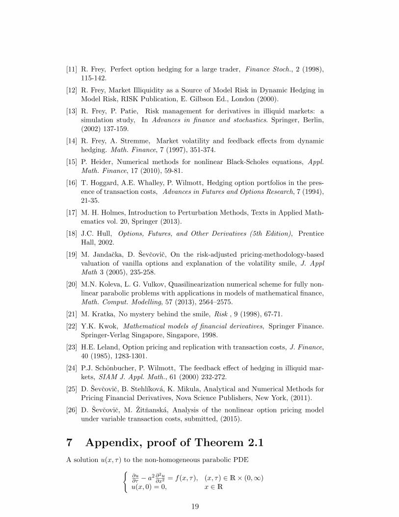
Numerical results from section 4 have demonstrated that the asymptotic formulacan be used for accurate approximation of a solution to the nonlinear Black-Scholesequation if the parameters ρ and µ are sufficiently small. From Figure 4, it is im-portant to notice that the option price increases for asset prices close to E whenthese parameters are increasing. In fact ρ and µ can be calibrated using marketdata to observe whether the market of underlying asset has high or low liquidity.

In the calibration experiments the parameter ρ for the Frey and Patie modelwas calibrated by using the call option time series from Apple Inc. (AAPL) inNASDAQ quotes market. Bisection method was used in the search algorithm asdescribed in Algorithm ??. The parameters in the calibration process were fixed asr = 0.01, E = 106, q = 0, and σ = σimpl was computed as the implied volatilityfrom the market quotes prices. As for the solution method (,Solver’) both analyticapproximation formula and Newton based methods were used. Table 7 shows similarcalibration results for both methods when the parameter ρ is not large using thesemarket data. This means that the analytic approximation formula has a benefit of

15

0 50 100 150 2000

5

10

15

20

time level

num

ber

of it

erat

ions

Number of iterations for NM1, NM2, Frozen Coefficient

NM1NM2Frozen

Figure 3: Number of iterations (vertical axis) for using NM1 (Blue), NM2 (Green) andfrozen coefficient (Red) in the Frey and Patie model for different times (horizontal axis).

90 95 100 105 1100

2

4

6

8

10

12

S

V(S

,t =

0)

Price with different values ρ

ρ = 0ρ = 0.025ρ = 0.05

90 95 100 105 1100

2

4

6

8

10

12

S

V(S

,t =

0)

Price with different values µ

µ = 0µ = 0.025µ = 0.05

Figure 4: Different option prices for ρ = 0, 0.025, 0.05 in the Frey and Patie model (left)and for µ = 0, 0.025, 0.05 in the RAPM model (right).

16

Table 7: Calibration results

τ S Vbid Vask σimpl ρAsym ρNewton

0.0753 107.67 6.100 6.200 0.443 3.807e-03 3.956e-030.0674 107.14 4.925 5.000 0.389 2.848e-03 2.934e-030.0595 112.37 8.225 8.300 0.401 3.492e-03 3.584e-030.0515 111.70 7.625 7.700 0.419 3.383e-03 3.347e-030.0436 109.01 6.225 6.300 0.506 2.939e-03 3.030e-030.0357 107.58 4.525 4.600 0.455 2.875e-03 2.995e-030.0277 110.37 5.950 6.000 0.458 2.228e-03 2.247e-030.0198 113.28 8.300 8.350 0.569 2.847e-03 2.912e-03

performing fast calibration when compared to Newton’s method.20 K. Ďuriš, S.-H. Tan, C.-H. Lai, D. Ševčovič

Algorithm 3: Model calibration with bisection search algorithmInput: Solver, Vask, tol, a = 0, b = 0.1Output: ρfor i = 1 : 100 do

1. ρ = a+b2 ;

2. if ‖Solver(S, τ, r, σimpl, ρ)− Vask‖ < tol thenbreak;else

if Solver(S, τ, r, σimpl, ρ)− Vask > 0 thenb = ρ ;else

a = ρ ;endgo back to 1.

endend

endend

Table 7. Calibration results

τ S Vbid Vask σimpl ρAsym ρNewton

0.0753 107.67 6.100 6.200 0.443 3.807e-03 3.956e-030.0674 107.14 4.925 5.000 0.389 2.848e-03 2.934e-030.0595 112.37 8.225 8.300 0.401 3.492e-03 3.584e-030.0515 111.70 7.625 7.700 0.419 3.383e-03 3.347e-030.0436 109.01 6.225 6.300 0.506 2.939e-03 3.030e-030.0357 107.58 4.525 4.600 0.455 2.875e-03 2.995e-030.0277 110.37 5.950 6.000 0.458 2.228e-03 2.247e-030.0198 113.28 8.300 8.350 0.569 2.847e-03 2.912e-03

6 Conclusion

In this paper two different linearization numerical methods for solving the nonlinearBlack-Scholes equation are proposed and analyzed. Numerical results are comparedin their accuracy and time complexity for the Frey and Patie illiquid market modeland the risk-adjusted pricing methodology model. It turns out that the analyticapproximation formula is more suitable for computation when the model parametersare sufficiently small. In particular it can be applied in calibrating parametersusing market data efficiently as it is a time consuming process for a full temporal-spatial finite difference approximation scheme based on Newton’s method. On theother hand, the analytic approximation formula becomes restrictive as the errorincreases when the parameters become larger. The Newton’s method is easy toimplement and suits various types of nonlinear Black-Scholes equations. There are

17

different approaches to implement Newton’s method and two of them are discussedin this paper. Although time complexity is a general problem, it can be improvedby combining other techniques or by using the so-called Newton-like methods toapproximate the Jacobian matrix in order to reduce the number of iterates. Bothtechniques in fact can be extended to solve other types of nonlinear option pricingmodels, and the resulting numerical solutions may also be considered as a benchmarksolution when exact solutions do not exist.

Acknowledgements

The authors thank Prof. Ljudmila A. Bordag for her kind suggestion about usingthe invariant solutions.

This research is supported by the European Union in the FP7-PEOPLE-2012-ITN project STRIKE - Novel Methods in Computational Finance (304617) and theSlovak research Agency Project VEGA 1/0780/15.

References

[1] P. Amster, C.G. Averbuj, M.C. Mariani, D. Rial, A Black–Scholes option pric-ing model with transaction costs. J. Math. Anal. Appl., 303 (2005), 688-695.

[2] M. Avellaneda, A. Paras, Dynamic hedging portfolios for derivative securitiesin the presence of large transaction costs. Appl. Math. Finance, 1 (1994),165-193.

[3] G. Barles, M.-H. Soner, Option pricing with transaction costs and a nonlinearBlack-Scholes equation. Finance Stoch., 2 (1998), 369-397.

[4] F. Black, M.S. Scholes, The Pricing of options and corporate liabilities, J.Political Economy, 81 (1973), 637-654.

[5] L.A. Bordag, R. Frey, Pricing options in illiquid markets: symmetry reduc-tions and exact solutions, Nonlinear Models in Mathematical Finance: NewResearch Trends in Option Pricing. Nova Science Publishers, Inc. New York(2008), pp.103-130.

[6] L.A. Bordag, Geometrical Properties of Differential Equations: Applicationsof the Lie Group Analysis in Financial Mathematics, World Scientific, (2015).

[7] R. Company, L. Jodar, J.R. Pintos, A consistent stable numerical scheme for anonlinear option pricing model in illiquid markets, Math. Comput. Simul., 82(2012), 1972-1985.

[8] R. Company, E. Navarro, J.R. Pintos, and F. Ponsoda, Numerical solution oflinear and nonlinear Black-Scholes option pricing equations. Comput. Math.Appl., 56 (2008), 813-821.

[9] M. Ehrhardt, Nolinear Models in Mathematical Finance, Nova Science Pub-lishers, Inc. New York (2008).

[10] M. Ehrhardt, R. Valkov, Numerical analysis of nonlinear European option pric-ing problem in illiquid markets, Preprint BUW-IMACM 14/23 (2014).

18

[11] R. Frey, Perfect option hedging for a large trader, Finance Stoch., 2 (1998),115-142.

[12] R. Frey, Market Illiquidity as a Source of Model Risk in Dynamic Hedging inModel Risk, RISK Publication, E. Gilbson Ed., London (2000).

[13] R. Frey, P. Patie, Risk management for derivatives in illiquid markets: asimulation study, In Advances in finance and stochastics. Springer, Berlin,(2002) 137-159.

[14] R. Frey, A. Stremme, Market volatility and feedback effects from dynamichedging. Math. Finance, 7 (1997), 351-374.

[15] P. Heider, Numerical methods for nonlinear Black-Scholes equations, Appl.Math. Finance, 17 (2010), 59-81.

[16] T. Hoggard, A.E. Whalley, P. Wilmott, Hedging option portfolios in the pres-ence of transaction costs, Advances in Futures and Options Research, 7 (1994),21-35.

[17] M. H. Holmes, Introduction to Perturbation Methods, Texts in Applied Math-ematics vol. 20, Springer (2013).

[18] J.C. Hull, Options, Futures, and Other Derivatives (5th Edition), PrenticeHall, 2002.

[19] M. Jandacka, D. Sevcovic, On the risk-adjusted pricing-methodology-basedvaluation of vanilla options and explanation of the volatility smile, J. ApplMath 3 (2005), 235-258.

[20] M.N. Koleva, L. G. Vulkov, Quasilinearization numerical scheme for fully non-linear parabolic problems with applications in models of mathematical finance,Math. Comput. Modelling, 57 (2013), 2564–2575.

[21] M. Kratka, No mystery behind the smile, Risk , 9 (1998), 67-71.

[22] Y.K. Kwok, Mathematical models of financial derivatives, Springer Finance.Springer-Verlag Singapore, Singapore, 1998.

[23] H.E. Leland, Option pricing and replication with transaction costs, J. Finance,40 (1985), 1283-1301.

[24] P.J. Schonbucher, P. Wilmott, The feedback effect of hedging in illiquid mar-kets, SIAM J. Appl. Math., 61 (2000) 232-272.

[25] D. Sevcovic, B. Stehlıkova, K. Mikula, Analytical and Numerical Methods forPricing Financial Derivatives, Nova Science Publishers, New York, (2011).

[26] D. Sevcovic, M. Zitnanska, Analysis of the nonlinear option pricing modelunder variable transaction costs, submitted, (2015).

7 Appendix, proof of Theorem 2.1

A solution u(x, τ) to the non-homogeneous parabolic PDE{∂u∂τ − a

2 ∂2u∂x2

= f(x, τ), (x, τ) ∈ R× (0,∞)u(x, 0) = 0, x ∈ R

19

is given by the variation of constant formula and is given by

u(x, τ) =

∫ τ

0

∫ ∞−∞

G(x− ξ, τ − s)f(ξ, s)dξ ds, where G(x, τ) =1√

4πa2τe−

x2

4a2τ .

The solution of equation (20) can be written

u(x, τ) =

∫ τ

0

∫ ∞−∞

1√2πσ2(τ − ξ)

e− (x−s)2

2σ2(τ−ξ)Eγ

(2πσ2ξ)δ2

A(ξ)

× e−δ

2σ2ξs2+[γ−δ−α(1−δ)]s−[β+qδ+ δ

2(1−α)2σ2]ξ

ds dξ.

Let us consider the change of variables in (22) and introduce the function:

R(ξ) =

[β + qδ +

δ

2(1− α)2σ2

]ξ = −β(δ − 1)ξ (28)

because β = − σ2

2 α2 − r (see (18)).

In order to simplify further notation and let EXP denote the power of theexponential function, i.e.

EXP =− x2 − 2xs+ s2

2σ2(τ − ξ)− δ

2σ2ξs2 + Ps−R(ξ)

=− ξ + δ(τ − ξ)2σ2(τ − ξ)ξ

s2 +

[x

σ2(τ − ξ)+ P

]s−R(ξ)− x2

2σ2(τ − ξ)

=− Q(τ, ξ)

2σ2(τ − ξ)ξ

s2 − 2x+ Pσ2(τ − ξ)

Q(τ, ξ)ξs+

[x+ Pσ2(τ − ξ)

Q(τ, ξ)ξ

]2

−

[x+ Pσ2(τ − ξ)

Q(τ, ξ)ξ

]2−R(ξ)− x2

2σ2(τ − ξ)

=− Q(τ, ξ)

2σ2(τ − ξ)ξ

{s− x+ Pσ2(τ − ξ)

Q(τ, ξ)ξ

}2

+

[x+ Pσ2(τ − ξ)

]22σ2(τ − ξ)Q(τ, ξ)

ξ

−R(ξ)− x2

2σ2(τ − ξ).

Consider the function Λ(τ, ξ) defined in (22). Then the inner integral can be calcu-lated as follows:

u(x, τ) =

∫ τ

0

EγA(ξ)

Λ(τ, ξ)exp

[x+ Pσ2(τ − ξ)

]22σ2(τ − ξ)Q(τ, ξ)

ξ −R(ξ)− x2

2σ2(τ − ξ)

×∫ ∞−∞

1√2πσ2(τ−ξ)ξQ(τ,ξ)

exp

− Q(τ, ξ)

2σ2(τ − ξ)ξ

[s− x+ Pσ2(τ − ξ)

Q(τ, ξ)ξ

]2 ds dξ

=

∫ τ

0

EγA(ξ)

Λ(τ, ξ)exp

[− δx2

2σ2Q(τ, ξ)+

Pxξ

Q(τ, ξ)+P 2σ2(τ − ξ)ξ

2Q(τ, ξ)−R(ξ)

]dξ.

20

Hence

u(x, τ) =

∫ τ

0

EγA(ξ)

Λ(τ, ξ)exp

{ξ −

[δτ + (1− δ)ξ

]2σ2(τ − ξ)

[δτ + (1− δ)ξ

]x2 +

[γ − δ − α(1− δ)

]xξ

δτ + (1− δ)ξ

+

[γ − δ − α(1− δ)

]2σ2(τ − ξ)ξ

2[δτ + (1− δ)ξ

] + β(δ − 1)ξ

dξ.

Now let us consider the case δ 6= 1. Since

ξ

δτ + (1− δ)ξ=

1

1− δδτ + (1− δ)ξ − δτδτ + (1− δ)ξ

=1

1− δ− δτ

1− δ1

δτ + (1− δ)ξ,

(τ − ξ)ξδτ + (1− δ)ξ

= Bξ + C +D

δτ + (1− δ)ξ,

where B = 11−δ , C = τ

(1−δ)2 and D = − δτ2

(1−δ)2 . Therefore

u(x, τ) =

∫ τ

0

EγA(ξ)

Λ(τ, ξ)exp

{− δx

2

2σ21

Q(τ, ξ)+

Px

1− δ− Pxδτ

(1− δ)Q(τ, ξ)+

P 2σ2ξ

2(δ − 1)

+P 2σ2τ

2(1− δ)2− P 2σ2δτ2

2(1− δ)2Q(τ, ξ)+ β(δ − 1)ξ

}dξ

=

∫ τ

0

EγA(ξ)

Λ(τ, ξ)exp

[

P 2σ2

2(δ − 1)+ β(δ − 1)

]ξ

+Px

1− δ+

P 2σ2τ

2(1− δ)2−

[δx2

2σ2+Pxδτ

1− δ+P 2σ2δτ2

2(1− δ)2

]1

Q(τ, ξ)

dξ.

Substituting the terms P,Q(τ, ξ),Λ(τ, ξ) yields the form of the solution u(x, τ) asstated in Theorem 2.1.

21