Embed Size (px)
Citation preview

Self-organization of Vectors
Wolfhard Hö[email protected]
AbstractPosition vectors, difference vectors and displacement vectors are linked by the dot product in a time discrete dynamical system in the n-dimensional Euclidean space. The algorithm presented here produces a variety of structures which are sometimes unstable and they may jump to other more stable attractors after a longer lifetime. First, consider two points (position vectors) in the space. The one point is displaced iteratively by a unit vector, and the second point by the same unit vector, however with reversed sign. Thus, the “center of mass” remains constant. The antiparallel displacement vectors lie on parallels, whose distance will be also kept unchanged. Hence the "torque" of the two points is also constant. Now, more points can be added. The points can be chosen freely combined to pairs of points. It results in a graph, the nodes of the graph correspond to the points, the edges correspond to the selected pairs of points. The executable program Attractor.jar demonstrates the variety of ways in which the vectors organize themselves spontaneously as a function of dimension and selected graph.
1
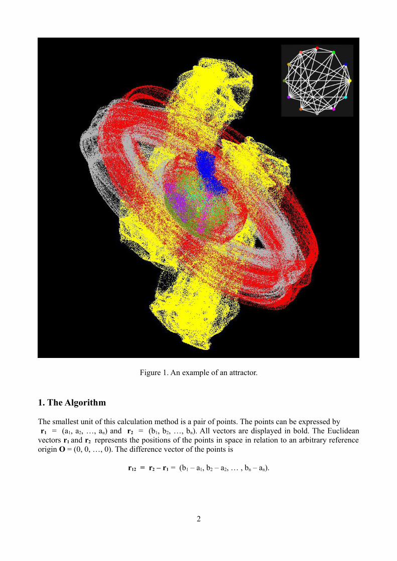
Figure 1. An example of an attractor.
1. The Algorithm
The smallest unit of this calculation method is a pair of points. The points can be expressed by r1 = (a1, a2, …, an) and r2 = (b1, b2, …, bn). All vectors are displayed in bold. The Euclidean vectors r1 and r2 represents the positions of the points in space in relation to an arbitrary reference origin O = (0, 0, …, 0). The difference vector of the points is
r12 = r2 – r1 = (b1 – a1, b2 – a2, … , bn – an).
2

Figure 2. Difference vector.
Now the two position vectors r1 and r2 are shifted by a displacement vector dr. Vector dr will be added to r1 and dr will be subtracted from r2. Thus the center of mass of the points (1, 2) remains constant. It might be useful but not necessary that the magnitude of dr is equal to 1, thus the displacement vector is always a unit vector.
Figure 3. Displacement of the points.
.
3
O
r1
r2r12
1
2
s
r
dr
-dr
1
2
12

The two points 1 and 2 are moving antiparallel along two parallels with the distance s, so the torque of the pair of points also remains constant. In order to prevent the system from diverging in further iterations an upper bound must be introduced. If the magnitude of the vector r12 exceeds the arbitrary bound e, the direction of dr is changed so that the torque s remains constant and the system does not diverge.Thereby e ≥ s always has to remain valid, since the distance of the points should not be smaller than the distance of the parallels. The new direction of the displacement vector dr has to lie on a tangent to the circle whose center is the same as the center of mass of the pair of points and whose radius is s/2. Thus, the constancy of torque is ensured. Here the displacement vector is practically reflected.
Figure 4. Reflection.
The displacement vector dra shifts towards the vector drb without change of the torque. The previous consideration applies only to a single pair of points. However, the algorithm gains interest when more points are added. Any new pairs of points can be chosen arbitrarily between the points. The crosslinking of the points can be represented by a graph, whereby the nodes of the graph correspond with the points and the edges correspond with the pairs of points. In case that a point is connected by more than one pair of points (in the graph multiple edges meet at a node ), all the corresponding displacement vectors must be added to that position vector.
For example, if a third point generates a new pair of points with point 1, there will be an additional shift of point 1 and the condition s = constant is no longer valid. Therefore, the geometry consideration needs to be expanded (Figure 5). The displacement vector dra is rotated around the point 1 in the following iteration, until its direction coincides with the tangent to the s-circle. Now the vector drb is the new displacement vector in respect of the pair of points 1 and 2. Thus the condition s = constant is fulfilled again. To facilitate the calculation, some abbreviations are introduced:
|r12| = r,
|dra| = |drb| = 1.
4
s
dr
-dr
1
2
a
a
drb
-drb
r12

Figure 5. Determination of the new displacement vector.
The vector y is equal to the sum of the vectors dra and x, where x is parallel to r12
y=dra+x .
The vector x is equal to the unit vector in the direction of r12 multiplied by the magnitude of x
x=r12
∣r12∣x=
r12
rx with ∣x∣= x .
An important role plays the dot product k that defines the angle between two vectors in the Euclidean space. First, the vectors r12 and dra are written in component form by
r 12=(r 1 , r 2 , ... , r n)dr a=(dr1 , dr2 ,... , drn) .
5
1
p/2
ba b-a
a
dr
dr
-dr
b
a
b
xy
r12
s/2
r/2
2
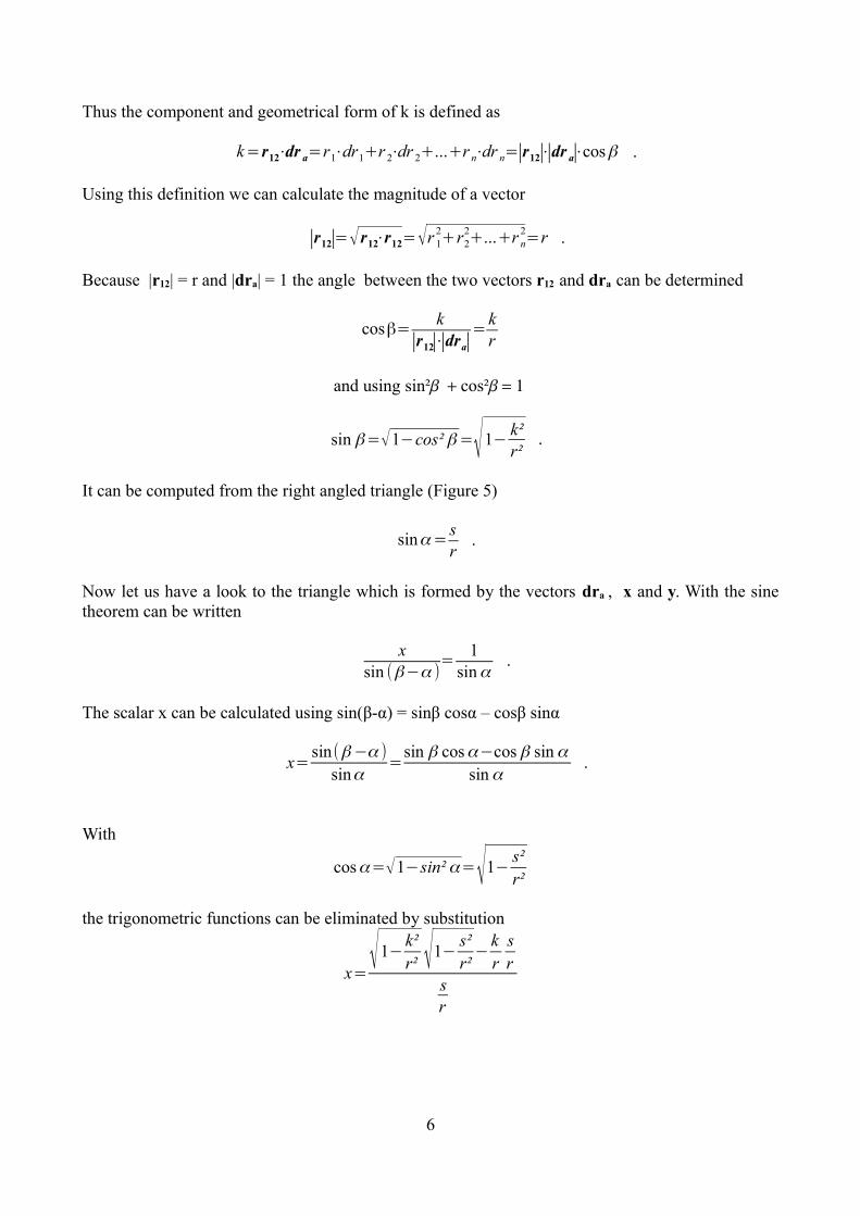
Thus the component and geometrical form of k is defined as
k=r12⋅dr a=r1⋅dr1+r 2⋅dr 2+...+r n⋅dr n=∣r12∣⋅∣dr a∣⋅cosβ .
Using this definition we can calculate the magnitude of a vector
∣r12∣=√r12⋅r12=√r 12+r2
2+...+r n
2=r .
Because |r12| = r and |dra| = 1 the angle between the two vectors r12 and dra can be determined
cosβ=k
∣r12∣⋅∣dra∣=kr
and using sin²b + cos²b = 1
sin β=√1−cos² β =√1−k²r²
.
It can be computed from the right angled triangle (Figure 5)
sinα=sr
.
Now let us have a look to the triangle which is formed by the vectors dra , x and y. With the sine theorem can be written
xsin (β−α )
=1
sinα.
The scalar x can be calculated using sin(β-α) = sinβ cosα – cosβ sinα
x=sin(β −α )
sinα=
sin β cosα−cos β sin α
sin α.
With
cosα=√1−sin²α=√1−s²r²
the trigonometric functions can be eliminated by substitution
x=√1−
k²r² √1−
s²r²
−krsr
sr
6

x=rs (√(1−
k²r² )(1−
s²r² )−
kr²s)
x=−kr+rs √(1−
k²r² )(1−
s²r² ) .
This implies the magnitude of the vector x
x=−kr+√( r²s²−1)(1−
k²r² )
and x is in the same direction as the vector r12
x=xr12
∣r12∣.
To get the vector y we have to add the two vectors dra and x. The direction of the vector y is the same as of the new displacement vector drb
y=dra+x=dr a+xr 12
∣r 12∣.
The vector drb is identical to the unit vector of y
dr b=y
∣y∣=
dra+x
∣dra+x∣.
2. Example Program AttracSimple
The equations implemented in an algorithm, this results in a relatively simple program. This will be demonstrated in the following example. The graph consists of the points (nodes) 1, 2 and 3. Between them two pairs of points (edges) 12 and 13 were selected.
Figure 6. Graph for AttracSimple.
7
1
2 3
12 13

The Java program AttracSimple shows the principle for three dimensions, other dimensions are simply possible by modifying the number of vector components in the source code. The parameter e defines the maximum magnitude of the difference vector between points. The parameter s determines the spacing of the parallels on which the antiparallel displacement vectors of a pair of points are located (Figure 3) and hence also the torque. Then, the initial values of the position vectors of the points are entered. For each pair of points, an initial displacement vector must be defined. This latter needs not be normalized, because it is always automatically converted into a unit vector.
package attracsimple;
public class AttracSimple { public static void main(String[] args) { // Parameters double e = 5.0, s = 3.0; // e >= s, s > 0
double radi, dr, x; //Initial conditions (x, y, z) double x1 = 0.01, y1 = -0.02, z1 = 0.04; double x2 = -0.04, y2 = -0.05, z2 = 0.01; double x3 = 0.05, y3 = -0.04, z3 = -0.01; double rq12, r12, scalar12, dx12 = 1.0, dy12 = -1.0, dz12 = 1.0; double rq13, r13, scalar13, dx13 = -1.0, dy13 = 1.0, dz13 = -1.0; int N = 15000; //steps
Now the iteration loop begins. After calculating the distance r12 between the points 1 and 2 the dot product r12·dr12 is determined. Then it is checked whether the upper bound is reached for the distance of the two points and also whether the magnitude of r12 exceeds the parameter s. If these conditions are met, the length of the auxiliary vector x is calculated. //Iteration loop---------------------------------------------------------- for(int i = 0; i < N; i++) { rq12 = (x2-x1)*(x2-x1)+(y2-y1)*(y2-y1)+(z2-z1)*(z2-z1); r12 = Math.sqrt(rq12); scalar12 = dx12*(x2-x1)+dy12*(y2-y1)+dz12*(z2-z1); if(r12 > e && r12 > s) { radi = (rq12/(s*s)-1.0)*(1.0-(scalar12*scalar12)/rq12); if(radi < 0.0) radi= 0.0; x = -scalar12/r12+Math.sqrt(radi);
First, the components of the vector y are determined. Then the unit vector of y is calculated. This is the new displacement vector which was searched for.
dx12 = dx12+x*(x2-x1)/r12; dy12 = dy12+x*(y2-y1)/r12; dz12 = dz12+x*(z2-z1)/r12; dr = Math.sqrt(dx12*dx12+dy12*dy12+dz12*dz12);
8

dx12 = dx12/dr; dy12 = dy12/dr; dz12 = dz12/dr; }
The same calculation is executed for the pair of points 1 and 3. In this case it would make sense to introduce methods or functions to avoid repetition of similar code, but here methods are not applied in order to ensure a better understanding.
rq13 = (x3-x1)*(x3-x1)+(y3-y1)*(y3-y1)+(z3-z1)*(z3-z1); r13 = Math.sqrt(rq13); scalar13 = dx13*(x3-x1)+dy13*(y3-y1)+dz13*(z3-z1); if(r13 > e && r13 > s) { radi = (rq13/(s*s)-1.0)*(1.0-(scalar13*scalar13)/rq13); if(radi < 0.0) radi = 0.0; x = -scalar13/r13+Math.sqrt(radi); dx13 = dx13+x*(x3-x1)/r13; dy13 = dy13+x*(y3-y1)/r13; dz13 = dz13+x*(z3-z1)/r13; dr = Math.sqrt(dx13*dx13+dy13*dy13+dz13*dz13); dx13 = dx13/dr; dy13 = dy13/dr; dz13 = dz13/dr; }
Now the two new displacement vectors are known. Thus, the new position vectors of the points are calculated. As for the point 1, two pairs of points must be taken into consideration, the vectors dr12
and dr13 are added to vector r1 . To the position vectors r2 and r3 the respective antiparallel displacement vectors are added. Then, the new points may be displayed.
//Superposition x1 = x1+dx12+dx13; y1 = y1+dy12+dy13; z1 = z1+dz12+dz13; x2 = x2-dx12; y2 = y2-dy12; z2 = z2-dz12; x3 = x3-dx13; y3 = y3-dy13; z3 = z3-dz13; //Position of node1, node2 and node3 System.out.format("%10f %10f %10f %10f %10f %10f %n", x1, y1, x2, y2, x3, y3); } }}
In the Annex the program AttracSimple is given once more coherently.
9

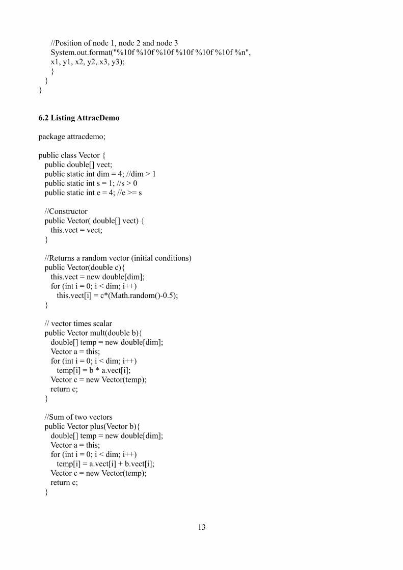
3. Example Program AttracDemo
As a second example the Java program AttracDemo shows how to define by means the class „Vector“ all necessary vector operations. In order to specify initial conditions, a random vector is constructed. Then the operations follow
Multiplying a vector by a scalarSum of two vectors
Difference of two vectorsDot product of two vectors
Magnitude of a vectorUnit vector of a vector
Reflection of a displacement vector.
Thus, any additional nodes and edges can be added to the algorithm. In the example the graph consists of three nodes and three edges. First, the three difference vectors are calculated. Then it is checked whether the upper bound is reached for the point distances and new displacement vectors must be determined. As a precaution it is verified whether the distance between the points is larger than the parameter s. Now may be determined the new positions of the points by superposing for each position vector the corresponding displacement vectors. In this example, for every position vector we have to add two displacement vectors, because every node is connected by two edges. The colored points 0, 1 and 2 are displayed on the screen after each iteration. In the Annex the program AttracDemo is given once more coherently.
Figure 7. Graph for AttracDemo.
/============================================================//Algorithm with vectors for( int i = 0; i < n; ++i){ r01 = r1.minus(r0); r02 = r2.minus(r0); r12 = r2.minus(r1); //Reflection? if (r01.mag() > Vector.e && r01.mag() > Vector.s) dr01 = r01.reflect(dr01); if (r02.mag() > Vector.e && r02.mag() > Vector.s) dr02 = r02.reflect(dr02); if (r12.mag() > Vector.e && r12.mag() > Vector.s) dr12 = r12.reflect(dr12);
10
0
1 2
01 02
12

// Superposition // node 0 (red) r0 = r0.plus(dr01); r0 = r0.plus(dr02); // node 1 (green) r1 = r1.minus(dr01); r1 = r1.plus(dr12); // node 2 (blue) r2 = r2.minus(dr02); r2 = r2.minus(dr12);//============================================================
4. The Program Attractor.jar
For the attached executable program Attractor.jar a maximum of 12 nodes and 66 edges is possible. In the Annex the graphical user interface will be explained in detail. The dimension n can be arbitrarily selected for n>1. The parameters e and s have a great influence on whether attractors may occur. A number of graphs are available, however, also random graphs can be generated and analyzed. Also of interest is the dynamic behavior of structures that can be better seen with the settings „Strobe“ and „Period“.
5. Self-organization
The described algorithm links together difference vectors and displacement vectors. It turns out that in many cases the vectors organize themselves spontaneously in form of specific structures. This effect can be observed even for graphs with 12 position vectors and 33 displacement vectors in the 7th dimension. In the example cited at least 547 vector components are interconnected and form the most diverse attractors. It seems that self-organization can occur more easily in higher dimensions.The attractors occur in different types of structures. The point cloud generated can converge towards more or less many fixed points. The „peaks“ of the position vectors sometimes describe closed curves or surfaces. Also diffuse structures are possible. These appear to be less stable because they can jump into simpler structures after many iterations.
6. Annex
6.1 Listing AttracSimple
package attracsimple;
public class AttracSimple { public static void main(String[] args) { // Parameters double e = 5.0, s = 3.0; // e >= s, s > 0
double radi, dr, x; //Initial conditions (x, y, z) double x1 = 0.01, y1 = -0.02, z1 = 0.04;
11

double x2 = -0.04, y2 = -0.05, z2 = 0.01; double x3 = 0.05, y3 = -0.04, z3 = -0.01; double rq12, r12, scalar12, dx12 = 1.0, dy12 = -1.0, dz12 = 1.0; double rq13, r13, scalar13, dx13 = -1.0, dy13 = 1.0, dz13 = -1.0; int N = 15000; //steps //Iteration loop---------------------------------------------------------- for(int i = 0; i < N; i++) { rq12 = (x2-x1)*(x2-x1)+(y2-y1)*(y2-y1)+(z2-z1)*(z2-z1); r12 = Math.sqrt(rq12); scalar12 = dx12*(x2-x1)+dy12*(y2-y1)+dz12*(z2-z1); if(r12 > e && r12 > s) { radi = (rq12/(s*s)-1.0)*(1.0-(scalar12*scalar12)/rq12); if(radi < 0.0) radi= 0.0; x = -scalar12/r12+Math.sqrt(radi); dx12 = dx12+x*(x2-x1)/r12; dy12 = dy12+x*(y2-y1)/r12; dz12 = dz12+x*(z2-z1)/r12; dr = Math.sqrt(dx12*dx12+dy12*dy12+dz12*dz12); dx12 = dx12/dr; dy12 = dy12/dr; dz12 = dz12/dr; } rq13 = (x3-x1)*(x3-x1)+(y3-y1)*(y3-y1)+(z3-z1)*(z3-z1); r13 = Math.sqrt(rq13); scalar13 = dx13*(x3-x1)+dy13*(y3-y1)+dz13*(z3-z1); if(r13 > e && r13 > s) { radi = (rq13/(s*s)-1.0)*(1.0-(scalar13*scalar13)/rq13); if(radi < 0.0) radi = 0.0; x = -scalar13/r13+Math.sqrt(radi); dx13 = dx13+x*(x3-x1)/r13; dy13 = dy13+x*(y3-y1)/r13; dz13 = dz13+x*(z3-z1)/r13; dr = Math.sqrt(dx13*dx13+dy13*dy13+dz13*dz13); dx13 = dx13/dr; dy13 = dy13/dr; dz13 = dz13/dr; } //Superposition x1 = x1+dx12+dx13; y1 = y1+dy12+dy13; z1 = z1+dz12+dz13; x2 = x2-dx12; y2 = y2-dy12; z2 = z2-dz12; x3 = x3-dx13; y3 = y3-dy13; z3 = z3-dz13;
12
//Position of node 1, node 2 and node 3 System.out.format("%10f %10f %10f %10f %10f %10f %n", x1, y1, x2, y2, x3, y3); } }}
6.2 Listing AttracDemo
package attracdemo;
public class Vector { public double[] vect; public static int dim = 4; //dim > 1 public static int s = 1; //s > 0 public static int e = 4; //e >= s
//Constructor public Vector( double[] vect) { this.vect = vect; }
//Returns a random vector (initial conditions) public Vector(double c){ this.vect = new double[dim]; for (int i = 0; i < dim; i++) this.vect[i] = c*(Math.random()-0.5); }
// vector times scalar public Vector mult(double b){ double[] temp = new double[dim]; Vector a = this; for (int i = 0; i < dim; i++) temp[i] = b * a.vect[i]; Vector c = new Vector(temp); return c; } //Sum of two vectors public Vector plus(Vector b){ double[] temp = new double[dim]; Vector a = this; for (int i = 0; i < dim; i++) temp[i] = a.vect[i] + b.vect[i]; Vector c = new Vector(temp); return c; }
13

//Difference of two vectors public Vector minus(Vector b){ double[] temp = new double[dim]; Vector a = this; for (int i = 0; i < dim; i++) temp[i] = a.vect[i] - b.vect[i]; Vector c = new Vector(temp); return c; }
// Dot product of two vectors public double dot(Vector b){ Vector a = this; double c = 0.0; for (int i = 0; i < dim; i++) c = c + a.vect[i] * b.vect[i]; return c; }
//Returns the magnitude of this vector. public double mag() { return Math.sqrt(this.dot(this)); }
//Returns the unit vector of this vector. public Vector unit() { double[] tmp = new double[dim]; double scalar = this.mag(); if (scalar > 0.0) scalar = 1.0 / scalar; for (int i = 0; i < dim; i++) tmp[i] = scalar * this.vect[i]; return new Vector(tmp); }
//Reflection at the boundary public Vector reflect(final Vector dre) { double r, rq, scalar, radi, x; rq = this.dot(this); if (rq < 1.0E-15) rq = 1.0E-15; r = Math.sqrt(rq); scalar = this.dot(dre); radi = (rq / (s*s) - 1.0) * (1.0 - scalar*scalar / rq); if (radi < 0) radi = 0; x = -scalar / r + Math.sqrt(radi); Vector dra = dre.plus(this.mult(x / r)).unit(); return dra; }}
14

package attracdemo;
import javax.swing.SwingUtilities;import javax.swing.JFrame;import javax.swing.JPanel;import java.awt.Color;import java.awt.Dimension;import java.awt.Graphics;
public class AttracDemo { public static void main(String[] args) { SwingUtilities.invokeLater(new Runnable() { @Override public void run() { createAndShowGUI(); } }); }
private static void createAndShowGUI() { JFrame f = new JFrame("AttracDemo"); f.setDefaultCloseOperation(JFrame.EXIT_ON_CLOSE); f.add(new MyPanel()); f.pack(); f.setVisible(true); }}
class MyPanel extends JPanel { public static Vector r0 = new Vector(0.1); public static Vector r1 = new Vector(0.1); public static Vector r2 = new Vector(0.1); public static Vector r01 = new Vector(0.0); public static Vector r02 = new Vector(0.0); public static Vector r12 = new Vector(0.0); public static Vector dr01 = new Vector(1.0); public static Vector dr02 = new Vector(1.0); public static Vector dr12 = new Vector(1.0); Color color0 = new Color( 255, 0, 0 ); Color color1 = new Color( 0, 255, 0 ); Color color2 = new Color( 0, 0, 255 ); public MyPanel() { setBackground(Color.BLACK); } @Override public Dimension getPreferredSize() { return new Dimension(800,800); }
15

@Override protected void paintComponent(Graphics g) { super.paintComponent(g);
//Paint specifications double zoom = 100.0; int x0 = 400; int y0 = 400; int n = 300000; //Number of pixels//============================================================//Algorithm with vectors for( int i = 0; i < n; ++i){ r01 = r1.minus(r0); r02 = r2.minus(r0); r12 = r2.minus(r1); //Reflection? if (r01.mag() > Vector.e && r01.mag() > Vector.s) dr01 = r01.reflect(dr01); if (r02.mag() > Vector.e && r02.mag() > Vector.s) dr02 = r02.reflect(dr02); if (r12.mag() > Vector.e && r12.mag() > Vector.s) dr12 = r12.reflect(dr12); // Superposition // node 0 (red) r0 = r0.plus(dr01); r0 = r0.plus(dr02); // node 1 (green) r1 = r1.minus(dr01); r1 = r1.plus(dr12); // node 2 (blue) r2 = r2.minus(dr02); r2 = r2.minus(dr12);//============================================================ //Draw Pixels g.setColor(color0); g.drawLine(x0 + (int)(zoom*(r0.vect[0])), y0 - (int)(zoom*(r0.vect[1])), x0 + (int)(zoom*(r0.vect[0])), y0 - (int)(zoom*(r0.vect[1]))); g.setColor(color1); g.drawLine(x0 + (int)(zoom*(r1.vect[0])), y0 - (int)(zoom*(r1.vect[1])), x0 + (int)(zoom*(r1.vect[0])), y0 - (int)(zoom*(r1.vect[1]))); g.setColor(color2); g.drawLine(x0 + (int)(zoom*(r2.vect[0])), y0 - (int)(zoom*(r2.vect[1])), x0 + (int)(zoom*(r2.vect[0])), y0 - (int)(zoom*(r2.vect[1]))); } }}
16

6.3 The graphical user interface for Attractor.jar
Figure 8. The graphical user interface for Attractor.jar.
New runNew initial conditions are given at random.
ClearThe screen content will be deleted.
ZoomThe screen content will be deleted and redrawn enlarged by a factor of 1.2 or reduced accordingly.
xMoving the image in x – direction.
yMoving the image in y – direction.
17

ProjectionThe attractor is projected from different directions onto the screen. The number of projections depends on the selected dimension.
All nodesAll points (position vectors) or only individual points are drawn. In this example program a maximum of 12 points are possible.
PullThe individual pairs of points are pulled apart with increasing intensity. This is accomplished by a vector which acts towards the direction of 45 degrees. Thereby different types of attractors may be generated.
NoiseThe points are shifted at random with increasing intensity in space. With this superimposed noise, the stability of the attractors can be checked.
DimensionThe dimension n of space can be set arbitrarily for n > 1.
Parameter eThe parameter e limits the maximum distance between the points of a pair of points.
Parameter sThe parameter s determines the distance of the parallels, on which lie the antiparallel displacement vectors of a pair of points.
Graph iHere you can select predefined graphs for which attractors were found. For the case graph i = 1 new graphs are continuously generated at random. If a new attractor is found, the search stops automatically.
Period = ii iterations will be performed and thereafter the calculated pixels are drawn.
StrobeThe screen is cleared before each period. With Period and Strobe the dynamic behavior of the attractors can be investigated.
Cross sectionFrom the structure a thin slice is cut out and displayed. The number of possible screen contents depends on the selected dimension.
GraphThe current graph, which determines the coupling of the nodes (position vectors) is displayed.
18