ALEA, Lat. Am. J. Probab. Math. Stat. 14, 445–471 (2017)

Self-exciting piecewise linear processes

Nikita Ratanov

Facultad de Economıa, Universidad del Rosario,Calle 12c, No.4-69Bogota, ColombiaE-mail address: nikita.ratanov@urosario.edu.co

URL: http://www.urosario.edu.co/Profesores/Listado-de-profesores/R/Nikita-Ratanov

Abstract. The paper concerns a piecewise linear process controlled by the set ofvelocities {cn}n≥0 consecutively switched after exponentially distributed, Exp(λn),n ≥ 0, time intervals. The distribution of such process is studied in detail, includingthe distribution of the first passage time through the constant boundary.

The processes which moves by alternating patterns and with a double jumpcomponent are also studied.

1. Introduction

A class of random processes with excitation at random times is studied for along time in various aspects. The main example of the process of that mannerof modeling is the telegraph process. On the physical parlance such process isalso called “steady-state random walks”. The telegraph processes describing non-interacting particles, which move with finite constant velocities switchable over anexponentially distributed random time intervals have been studied by many authorsbeginning with Taylor (1922).

This model with the alternating velocities ±c has been later developed by Gold-stein (1951) in connection with hyperbolic partial differential equations. In 1956Mark Kac began to study the telegraph model in detail, see Kac (1974). The distri-bution density p = p(x, t) of the particles’ positions follows the telegraph (dampedwave) equation

∂2p

∂t2+ 2λ

∂p

∂t= c2

∂2p

∂x2, (1.1)

where λ is the switching intensity.Afterwards, the telegraph process has been studied in great detail with many

generalisations. In particular, the motions with the velocities alternating in gamma-

Received by the editors July 19th, 2016; accepted May 6th, 2017.2010 Mathematics Subject Classification. 60J75, 60K15.Key words and phrases. piecewise linear process, steady-state random walk, jump-telegraph

process, first passage time, martingales.

445

446 N. Ratanov

or Erlang-distributed random intervals have been studied many times, see e. g.Di Crescenzo (2001); Zacks (2004); Di Crescenzo and Martinucci (2010). Motionscharacterised by more then two possible deterministic velocities (Orsingher andBassan, 1992; Kolesnik, 1998; Samoılenko, 2002) or random velocities (Stadje andZacks, 2004; Lopez and Ratanov, 2012) have been also considered.

Here we present the similar processes L = L(t), t ≥ 0, with the sequentialvelocities, {cn}n≥0, switched by the successive intensities {λn}n≥0. The modelis based on piecewise-deterministic Markov processes which originally have beendesigned for queueing theory, see Gnedenko and Kovalenko (1968). These modelsare used in various fields, see Costa and Davis (1989); Davis (1984); de Saporta andDufour (2012). Instead of PDE (1.1), by conditioning on the first switching one caneasily get integral equations for distributions of these processes, see equations (2.10)and (3.13). However, a detailed analysis of the distributions of these processes stillwas not done.

These processes can be considered as an example of self-exciting Hawkes pro-cesses well-studied before, beginning with the seminal paper by Hawkes (1971).Recently the Hawkes processes are intensively applied in finance, see e.g. Em-brechts et al. (2011). See also an overview by Bacry et al. (2015). In the context ofmarket model based on Hawkes processes the optimal execution problem is solvedexplicitly by Alfonsi and Blanc (2016).

This presentation continues the author’s paper Ratanov (2014), where the ex-plicit formula for the moment generating function of the piecewise linear processL(t), t > 0, was given. The distributions of these processes are studied in Section2, including the distribution of the first passage time T (x) (for the process withpositive velocities, where the level x is also positive, see Section 2.2). In Section 2.3we derive explicit formulae for the expectations of L(t) with jumps rn, occurringafter each velocity switching.

Section 3 presents the piecewise linear processes, which are developing in ac-cordance with alternately changing patterns. These processes are supplied with adouble jump component. First, there is a jump immediately after each velocityswitching (during the current pattern). Second, a jump accompanies the patternschanging. In the latter case a jump amplitude depends on the number of the ve-locity switchings during the current pattern. The system of integral equations forexpectations of such process X = X(t) is obtained. Further, there are describedmartingales of this form.

Telegraph-like processes have multiple applications including the applications tofinancial market modelling, see Di Mazi et al. (1994), and then, Ratanov (1999);Di Crescenzo and Pellerey (2002). Nowadays, these applications became the theoryof Markov-modulated market models based on telegraph processes with alternatingvelocities, see e. g. Ratanov (2007, 2010); Lopez and Ratanov (2014) (see also thesurvey in Kolesnik and Ratanov, 2013).

It has long been clear that for the purpose of financial modelling a simple replace-ment of a Wiener process on a telegraph usually produces arbitrage opportunitiessince the (stochastic) exponential of a telegraph process is not a martingale. Toresolve the problem, one can study the model with jump and/or diffusion compo-nent, Kolesnik and Ratanov (2013); Ratanov (2010). However, erroneous modelsbased only on the telegraph process continue to appear in publications, see e.g.De Gregorio (2016, Section 4).

Self-exciting piecewise linear processes 447

A sketch of the financial market model based on the double-jump process withalternately changing piecewise linear patterns is presented in Section 4. This modelinvolves switching tendencies (accompanied by jumps of random amplitude) dueto the internal market forces (small investors). Meanwhile, switching between thepatterns is determined by a regulator policy (or an institutional/strategic investor).It turns out that a certain policy of the strategic investor could provoke arbitrage.

2. Jump-telegraph processes with distinct parameters

We repeatedly use the following notations.

Let ~c = {cn}n≥0 and ~λ = {λn}n≥0 be two numerical sequences. Assume that allpairs 〈cn, λn〉, n ≥ 0, are distinct, i. e., if for l 6= k, cl = ck, then λl 6= λk. Theproducts

κn,k(~c, ~λ) =n∏

l=0, cl 6=ck

(cl − ck)−1 ×n∏

l=0, cl=ckl 6=k

(λl − λk)−1, (2.1)

n ≥ 1, 0 ≤ k ≤ n,are well-defined; κ0,0 = 1. If all cn are distinct, ck 6= cn for k 6= n, then we use theshortened notation,

κn,k(~c) =

n∏j=0, j 6=k

(cj − ck)−1, n ≥ 1, 0 ≤ k ≤ n. (2.2)

Note that due to the known Vandermonde properties, for n ≥ 1n∑k=0

κn,k(~c)cmk

(z + ck)=

zm

Πn(z), 0 ≤ m ≤ n, (2.3)

(if ck 6= cn for k 6= n), where Πn(z) = Πn(z;~c) =∏nk=0(z + ck). Hence,

n∑k=0

κn,k(~c)cmk = 0, 0 ≤ m ≤ n− 1.

Moreover,n∑k=0

κn,k(~c)cnk = (−1)n,

Kuznetsov (2003, p.11), see also Ratanov (2014, Remark 1 and (2.8)-(2.9)).In what follows we assume

∑A · = 0 and

∏A · = 1 if A = ∅.

2.1. Piecewise linear process. In this paper we study the continuous piecewise linearprocess L = L(t), t ≥ 0,

L(t) =

∫ t

0

cN(u)du =

N(t)−1∑n=0

cnτn + cN(t)(t− τ+,N(t))

=

N(t)−1∑n=0

(cn − cN(t))τn + cN(t)t,

(2.4)

which corresponds the position of a particle moving with successive velocities cn,switching after elapsed times τn. Here τ+,n denotes the switching instants, τ+,n =∑n−1k=0 τk, n ≥ 1, τ+,0 = 0, and N = N(t) is the corresponding counting process.

448 N. Ratanov

Let π(t;n), n ≥ 0, be the probability mass function, π(t;n) = P{N(t) = n}.The expectation of L(t), t ≥ 0, can be expressed by

E[L(t)] =

∫ t

0

E[cN(u)]du =

∞∑n=0

cn

∫ t

0

π(u;n)du, (2.5)

if the series converges.Let τn be independent and exponentially distributed, τn ∼ Exp(λn), λn > 0,

n ≥ 0.The probability mass functions π(t;n) = P{N(t) = n} satisfy the system,

dπ(t;n)

dt= −λnπ(t;n) + λn−1π(t;n− 1), t > 0; n ≥ 1 (2.6)

and π(t; 0) = e−λ0t, t ≥ 0, see Feller (1950).Random variables τ+,n, n ≥ 1, are Erlang-distributed. If all λ′s are distinct,

then the density function ϕn(t) of τ+,n is given by

ϕn(t) = Λn

n−1∑k=0

κn−1,k(~λ)e−λkt1{t>0}, n ≥ 1, (2.7)

Here Λn = Πn−1(0;~λ) =∏n−1k=0 λk, n ≥ 1, Λ0 = 1, and κn−1,k(~λ) are defined by

(2.2). The usual modifications can be applied if two or more λk are equal. For

instance, ϕn(t) =λntn−1

(n− 1)!e−λt1{t>0}, if λn ≡ λ, n ≥ 0.

If all λ′s are distinct, then by (2.7) the probability mass function of N(t), t > 0,is given by

π(t;n) = P{N(t) = n} =P{τ+,n+1 > t} − P{τ+,n > t}

=Λn

n∑k=0

κn,k(~λ)e−λkt, n ≥ 0,(2.8)

with the usual modifications, if some of λk are equal. Cf. Ratanov (2014, (2.4)).It’s known that process N is non-explosive, P{limn→∞ τ+,n = ∞} = 1, if and

only if ∑n≥0

λ−1n =∞, (2.9)

see Feller (1950, XVII.4). Examples of explosive processes can be found e.g. inSnyder and Miller (1991), see Example 6.3.1 with λn = (n+ 1)2.

Let 〈cn, λn〉, n ≥ 0, be the sequence of states of the process L = L(t).We find an explicit formula for the density function p = p(x, t) of L(t) in the

form

p(x, t) =

∞∑n=0

pn(x, t), x ∈ (−∞,∞), t ≥ 0.

Here pn(·, t) are the density functions of L(t)1{N(t)=n}, which are determined bythe set of n+ 1 states {〈ck, λk〉 | k = 0, . . . , n}.

Note that if there are no switchings, N(t) = 0, L(t) = c0t, then the distributionof L(t)1{N(t)=0} corresponds to Dirac’s δ-measure located at c0t (with probability

Self-exciting piecewise linear processes 449

π(t; 0) = e−λ0t), i. e., p0(x, t) = e−λ0tδ(x− c0t). Moreover, functions pn follow theset of integral equations, n ≥ 1

pn(x, t) = λ0

∫ t

0

e−λ0upn−1(x− c0u, t− u)du, (2.10)

where pn−1 are determined by the set parameters {〈ck, λk〉 | k = 1, . . . , n}, begin-ning with 〈c1, λ1〉.

The detailed properties and the explicit formulae for the distributions of L(t),t ≥ 0, with the states 〈c0, λ0〉 and 〈c1, λ1〉, alternating at times τ+,n, n ≥ 0, areknown. The density functions pn(x, t) of L(t)1{N(t)=n}, n ≥ 1, are given by

pn(x, t) =λ

[(n+1)/2]0 λ

[n/2]1

[n/2]! [(n− 1)/2]!τ∗

[n/2](t− τ∗)[(n−1)/2]

× exp(−λ0τ∗ − λ1(t− τ∗))c0 − c1

1{0<τ∗<t},

where τ∗ =x− c1tc0 − c1

, t − τ∗ =c0t− xc0 − c1

, [·] denotes the integer part and the initial

state is 〈c0, λ0〉. See Kolesnik and Ratanov (2013, Chapter 4), where system (2.10)is solved for the case of alternating states.

This result can be also obtained by using the moment generating functions

ψn(z, t) = E{ezL(t)1{N(t)=n}}, n ≥ 1.

The explicit formulae for ψn see in Lopez and Ratanov (2014, Theorem 2.1).In this paper we study the distribution of L(t), when all states 〈cn, λn〉, n ≥ 0,

are distinct. By Ratanov (2014, Theorem 3.1) in this case the moment generatingfunctions are

ψn(z, t) = E{ezL(t)1{N(t)=n}} = Λn

n∑k=0

κn,k(λ)e−λkt, n ≥ 1. (2.11)

Here the linear functions λk = λk(z) = λk − ckz, 0 ≤ k ≤ n, are distinct, and |z| issufficiently small, such that all λk(z) remain to be positive, λk(z) > 0, 0 ≤ k ≤ n.The latter means that

if ck > 0, then z < λk/ck; if ck < 0, then z > λk/ck, 0 ≤ k ≤ n. (∗)

If some of states are equal, formula (2.11) can be modified.It is easy to see that

κn,k(λ) =

n∏j=0, j 6=k

(λj − λk − z(cj − ck))−1

= κn,k(~c, ~λ) ·n∏j=0

cj 6=ck

(bj,k − z)−1,

where κn,k(~c, ~λ) are defined by (2.1) and bj,k =λj − λkcj − ck

, if cj 6= ck. Hence, by

(2.11)

ψn(z, t) = Λn

n∑k=0

κn,k(~c, ~λ)e−λkt × ezckt∏nj=0, cj 6=ck(bj,k − z)

(2.12)

for z satisfying condition (*). The distribution of L(t) can be obtained by in-verse Laplace transformation of (2.12), i. e., one can find the density function pn

450 N. Ratanov

satisfying the equation ∫ ∞−∞

ezxpn(x, t)dx = ψn(z, t).

Throughout the paper we will use the notations:

Bj,k = −bj,kck + λk =λkcj − λjckcj − ck

, and τj,k = τj,k(x, t) =x− cktcj − ck

, (2.13)

cj 6= ck, j, k ≥ 0.

Notice that bj,k = bk,j , Bj,k = Bk,j , τj,k(x, t) + τk,j(x, t) ≡ t and

λjτj,k(x, t) + λkτk,j(x, t) ≡ bj,kx+Bj,kt ≡ bj,k(x− ckt) + λkt, (2.14)

cj 6= ck, j, k ≥ 0.

We will consider two cases:

A1: all bj,k are distinct, if they are defined:bl,k 6= bj,k ( for all l 6= j, cl 6= ck, cj 6= ck);

B1: all bj,k are identical, bj,k = β, 0 ≤ j, k ≤ n (for cj 6= ck).

By applying (2.3) one can notice that in case A1 the moment generating functionψn, (2.12), becomes

ψn(z, t) = Λn

n∑k=0

κn,k(~c, ~λ)e−λkt ×n∑j=0

cj 6=ck

κn,j(~bk)ezckt

bj,k − z. (2.15)

Here κn,j(~bk) is defined similarly to (2.2),

κn,j(~bk) =

n∏l=0, l6=j,

cl 6=ck,cj 6=ck

(bl,k − bj,k)−1. (2.16)

Note that in case B1 functions

λjτj,k(x, t) + λkτk,j(x, t) ≡ λkt+ β(x− ckt), j ∈ {0, . . . , n},do not depend on j, see (2.14). Moreover, in this case by (2.12) ψn(z, t) becomes

ψn(z, t) = Λn

n∑k=0

κn,k(~c, ~λ)e−λkt × ezckt

(β − z)m(2.17)

The following theorem proposes some explicit formulae for the density functionspn = pn(x, t) of L(t)1{N(t)=n}, t > 0, n ≥ 1.

Theorem 2.1. • In case A1:

pn(x, t) = Λn

n∑k,j=0,

cj 6=ck

φckt,bj,k(x)κn,k(~c, ~λ)κn,j(~bk) · exp(−λjτj,k(x, t)− λkτk,j(x, t)).

(2.18)• In case B1:

pn(x, t) = Λn

n∑k=0

φckt,β(x)κn,k(~c, ~λ) · (x− ckt)m

m!exp(−λkt− β(x− ckt)). (2.19)

Here for each k, k ∈ {0, . . . , n}, we denote by m = mn,k the number of j,j ∈ {0, . . . , n}, such that cj 6= ck.

Self-exciting piecewise linear processes 451

Function φa,b(x) is defined in Appendix,

φa,b(x) =

{1{x>a}, if b > 0,

−1{x<a}, if b < 0.

Proof : In cases A1 and B1 we apply the inverse Laplace transform to functionsψn(·, t), defined by (2.15) and (2.17) respectively. Formulae (2.18)-(2.19) follow byProposition 1 of Appendix.

If all bj,k are distinct, then by (2.15) and formula (1) of Appendix we obtain

pn(x, t) = Λn

n∑k,j=0,

cj 6=ck

κn,k(~c, ~λ)e−λktφckt, bj,k(x)κn,j(~bk) exp (−bj,k(x− ckt)) . (2.20)

Moreover, bj,k(x− ckt) + λkt = bj,kx+Bj,kt ≡ λjτjk(x, t) + λkτkj(x, t).Similarly, (2.19) follows from (2.17) and formula (1) of Appendix. �

Remark 2.2. In a situation comprised between the extreme cases A1 and B1 similarformulae can also be obtained. This is the usual modifications based on partialfraction decomposition of ψn, which can be applied if some (not all) of bj,k areequal.

Remark 2.3. By definition (2.4) after n steps the support of random variable L(t)is compact. If N(t) = n, then

L(t) ∈ [ant, Ant], ∀t, t > 0, n ≥ 1.

Here an = min0≤k≤n

{ck}, An = max0≤k≤n

{ck}.

By using representation (2.18) one can also show

P{L(t) ∈ [ant, Ant] | N(t) = n} = 1, t > 0, n ≥ 1, (2.21)

(in the case of distinct bj,k). Indeed, it is easy to see that

κn,k(~c, ~λ)κn,j(~bk) + κn,j(~c, ~λ)κn,k(~bj) = 0, j, k ∈ {0, . . . , n}, j 6= k, n ≥ 1.

Therefore, (2.18) can be transformed to

pn(x, t) = Λn

n∑k,j=0

k<j, cj 6=ck

|κn,k(~c, ~λ)κn,j(~bk)|ej,k(x, t),

where

ej,k(x, t) ≡ ek,j(x, t) = exp(−λjτj,k(x, t)− λkτk,j(x, t))1{x is between cjt and ckt}.

This gives (2.21).Further, by the definition we have∫ ∞

−∞pn(x, t)dx = π(t;n) = P{N(t) = n}, n ≥ 1.

452 N. Ratanov

This also follows by integrating in (2.18) and (2.19). Indeed, if all bj,k are distinct,

by (2.20) and (2.3) (with ~bk instead of ~c) one can obtain∫ ∞−∞

pn(x, t)dx =Λn

n∑k,j=0, cj 6=ck

e−λktκn,k(~c, ~λ)κn,j(~bk)b−1j,k

=Λn

n∑k=0

e−λktκn,k(~c, ~λ)

n∏j=0, cj 6=ck

b−1j,k

= Λn

n∑k=0

κn,k(~λ)e−λkt

=π(t;n).

In the case of identical bj,k the same observations similarly follow from (2.19).

Figure 2.1. Density functions p(x, t) with cn = 1+(−1)n ln(n+1)and λn = 2 and t = 1, 2, 3 (from left to right).

Figure 2.1 displays the density functions in the case of slowly accelerating move-ment with reversals, cn = (−1)n ln(n+ 1) (the switching intensity is constant).

Next, we present some other examples.

Example 2.4. Consider an accelerating movement with linearly increasing velocitiesand switching intensities.

Let cn = c(n+ 1) and λn = λ(n+ 1), n ≥ 0.

Self-exciting piecewise linear processes 453

Figure 2.2. Density functions p(x, t) with cn = n + 1 and λn =n+ 1 and t = 1, 1.5, 2 (from left to right).

In this case bj,k ≡ λ/c, Bj,k ≡ 0, κn,k(~c) =(−1)k

cnk!(n− k)!, Λn = λnn! and by

(2.19)

pn(x, t) = n(λ/c)ne−λx/cn∑k=0

(−1)k(x− ckt)n−1

k!(n− k)!1{x>ckt}, n ≥ 1.

Therefore, the absolutely continuous part of the distribution of L(t) can be simpli-fied by

∞∑n=1

pn(x, t) = e−λx/c∞∑n=1

n(λ/c)nn∑k=0

(−1)k(x− ckt)n−1

k!(n− k)!1{x>ckt}

=λ

ce−λt1{x>ct}+e−λx/c

∞∑k=1

(−1)k

k!1{x>ckt}

[ ∞∑n=k

n(λ/c)n

(n− k)!(x− ckt)n−1

]

=λ

ce−λt1{x>ct}+

λ

ce−λx/c

∞∑k=1

(−1)k

k!ηk(x, t)k−11{x>ckt}

∞∑n=0

(n+ k)ηk(x, t)n

n!,

where ηk(x, t) = λ(x− ckt)/c.

454 N. Ratanov

By summing up in the latter series one can obtain the density function p = p(x, t)of L(t),

p(x, t) = e−λt

[δ(x− ct) +

λ

c

∞∑k=0

(−1)kηk(x, t)k−1

k!(k + ηk(x, t)) e−kλt1{x>ckt}

].

(2.22)Notice that for fixed x and t the sum in (2.22) is of finite number of terms. Figure

2.2 shows the absolutely continuous part of the density function p(x, t) defined by(2.22).

Example 2.5. Consider an accelerating movement with linearly increasing velocitiesand constant intensities.

Figure 2.3. Density functions p(x, t) with cn = n+ 1 and λn = 1and t = 1, 1.5, 2 (from left to right).

Let cn = c(1 + n), c > 0, and λn ≡ λ, n ≥ 0. In this case the density functionp = p(x, t) =

∑∞n=0 pn(x, t) of L(t), t > 0, can be simplified up to

p(x, t) = e−λt

[δ(x− c0t)

+λ

c

∞∑k=0

(−1)kηk(x, t)(k−1)/2

k!Ik−1

(2√ηk(x, t)

)1{x>ckt}

],

(2.23)

where Iν = Iν(z) =∑∞n=0

(z/2)ν+2n

n!Γ(ν+n+1) , ν ≥ 0; I−1 = I1 are modified Bessel func-

tions; ηk(x, t), k ≥ 0, are defined in Example 2.4.

Self-exciting piecewise linear processes 455

Indeed, by (2.19) the functions pn, n ≥ 1, become

pn(x, t) =(λ/c)n

(n− 1)!e−λt

n∑k=0

(−1)k(x− ckt)n−1

k!(n− k)!1{x>ckt}.

Therefore,

p(x, t) =

∞∑n=0

pn(x, t)

=e−λt[δ(x− c0t) +

∞∑n=1

(λ/c)n

(n− 1)!

n∑k=0

(−1)k(x− ckt)n−1

k!(n− k)!1{x>ckt}

]=e−λt

[δ(x− c0t) +

∞∑n=1

(λ/c)n

(n− 1)!n!(x− ct)n−11{x>ct}

+

∞∑k=1

(−1)k

k!1{x>ckt}

∞∑n=k

(x− ckt)n−1

(n− 1)!(n− k)!(λ/c)n

],

(2.24)

which by definition of Iν gives (2.23).Notice that for fixed x and t the sum in (2.23) is of finite number of terms. Figure

2.3 represents the absolutely continuous part of the density functions expressed by(2.24).

Example 2.6. Let L = L(t) be a process with alternating velocities c2n = c, c2n+1 =−v, n ≥ 0, and with switching intensities, λ2n = λ(1 + n), λ2n+1 = µ(1 + n),λ, µ > 0. This example has been analysed in detail by Di Crescenzo and Martinucci(2010).

Formulae (2.18) enable to repeat their result and, moreover, solve the unsolvedPDEs, written at the beginning of Section 3 in Di Crescenzo and Martinucci (2010).

One can see that in this case the coefficients in (2.18) are given by

Λ2n =λnµn(n!)2, Λ2n+1 = λn+1µnn!(n+ 1)!

τ2k,2j+1 =x+ vt

c+ v, τ2j+1,2k = t− τ2k,2j+1 =

ct− xc+ v

,

b2j,2k+1 =λ(1 + j)− µ(1 + k)

c+ v,

b2j+1,2k =λ(1 + k)− µ(1 + j)

c+ v,

κ2n,2k(~c, ~λ) =(−1)n+k(c+ v)−nλ−n[k!(n− k)!]−1,

κ2n,2k+1(~c, ~λ) =(−1)k(c+ v)−n−1µ−n+1[k!(n− k − 1)!]−1,

κ2n+1,2k(~c, ~λ) =(−1)n+k(c+ v)−n−1λ−n[k!(n− k)!]−1,

κ2n+1,2k+1(~c, ~λ) =(−1)k(c+ v)−n−1µ−n[k!(n− k)!]−1,

κ2n,2j+1(~b2k) =(−1)n−j−1(c+ v)n−1µ−n+1[j!(n− j − 1)!]−1,

κ2n+1,2j+1(~b2k) =(−1)n−j(c+ v)nµ−n[j!(n− j)!]−1,

κ2n,2j(~b2k+1) =κ2n+1,2j(~b2k+1) = (−1)j(c+ v)nλ−n[j!(n− j)!]−1,

(2.25)

for n, k, j ∈ {0, . . . , n}.

456 N. Ratanov

By summing up in (2.18) with (2.25) we get, for −vt < x < ct

p2n(x, t) =nµ

c+ ve−λτ∗−µ(t−τ∗)(1− e−λτ∗)n(1− e−µ(t−τ∗))n−1, n ≥ 1, (2.26)

p2n+1(x, t) =(n+ 1)λ

c+ ve−λτ∗−µ(t−τ∗)(1− e−λτ∗)n(1− e−µ(t−τ∗))n, n ≥ 0. (2.27)

Here τ∗ =x+ vt

c+ v.

Furthermore, functions p2n = fn(x, t | c) and p2n+1 = bn(x, t | c) defined by(2.26)-(2.27) solve PDEs of Di Crescenzo and Martinucci (2010, p.88). Functionsfn(x, t | − v) and bn(x, t | − v) can be written similarly.

Formulae Di Crescenzo and Martinucci (2010, (3.5)-(3.6)) for the density func-tions f(x, t | c) =

∑∞n=1 p2n(x, t) and b(x, t | c) =

∑∞n=0 p2n+1(x, t) easily follow

from (2.26) and (2.27). Multiple plots depicting the density functions p = p(·, t)with different λ, µ and t are as well presented by Di Crescenzo and Martinucci(2010).

Figure 2.4. Density functions p(x, t) with cn = (−2/3)n andλn = 3 and t = 1, 2, 3 (from top to bottom).

Example 2.7. Consider the fading case, cn = (−a)n, 0 < a < 1, and λn ≡ λ,λ > 0, n ≥ 0. By (2.19) we have

pn(x, t) =λne−λt

(n− 1)!

n∑k=0

κn,k(~c)(x− ckt)n−11{x > ckt}, n ≥ 1. (2.28)

Self-exciting piecewise linear processes 457

In this case by “three-series theorem” L(t) converges a. s., as t → ∞. The distri-bution of L(∞) is given by

P{L(∞) < x} =

∫ ∞0

[1− F

(y − xa

)]dF (y),

where

F (x) =

[1− s−1

∞∑n=0

(−1)nAne−λx/a2n

]1{x≥0}, s =

∞∑n=0

(−1)nAn.

Here An =an(n+1)

(1− a2)n(n+1)/2, cf Samoılenko (2002).

Figure 2.4 displays the absolutely continuous part of the density functions of thefading movement, defined by (2.28).

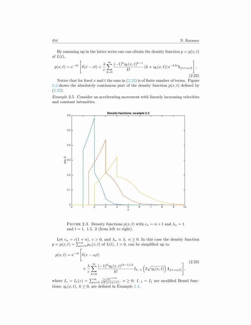
2.2. First passage time. Let x, x > 0, and T = T (x) be the first passage time

T (x) = inf{t ≥ 0 | L(t) = x}. (2.29)

In the case of alternating parameters, cn ∈ {c0, c1}, λn ∈ {λ0, λ1}, c0 > 0 >c1, the distribution of T (x) is well-studied. See Foong (1992), Foong and Kanno(1994), Orsingher (1995) and Pinsky (1991) for symmetric processes, (λ0 = λ1

and c0 = −c1), Stadje and Zacks (2004) and Lopez and Ratanov (2014, Theorem3.1) in the asymmetric case. The case of alternating velocities c, −v with linearlyincreasing reversal rates is studied by Di Crescenzo and Martinucci (2010).

Here we study the distribution of T (x) assuming all velocities cn to be positive.Under the non explosion condition, see (2.9),

∞∑n=0

cnλn

=∞, (2.30)

we have T (x) <∞, a.s. Notice that cnτn is exponentially distributed, Exp(λn/cn),n ≥ 0.

The distribution of T (x) possesses an atom at x/c0,

P{T (x) = x/c0} = e−λ0x/c0 .

We compute the absolutely continuous part of the distribution in the following twocases:

A2: all Bj,k are distinct, if they are defined:Bl,k 6= Bj,k ( for all l 6= j, cl 6= ck, cj 6= ck);

B2: all Bj,k are identical, Bj,k = B, 0 ≤ j, k ≤ n (for cj 6= ck).

Here Bj,k are defined by (2.13).It is easy to see, that in the case B2 all bj,k are also equal: bj,k ≡ β.Let gn(t;x) be the density function of the random variable T (x)1{N(T (x))=n},

n ≥ 1.

Theorem 2.8. Let cn > 0 ∀n, and condition (2.30) be hold. The density functionsgn(t;x) are given by

• in case A2:

gn(t;x) = −Λncn

n∑k,j=0

cj 6=ck

cm−1k κn,k(~c, ~λ)κn,j(− ~Bk)e−(Bj,kt+bj,kx)1{ckt>x}, (2.31)

458 N. Ratanov

where coefficients κn,j( ~Bk) are defined by (2.16);• in case B2:

gn(t;x) = −Λncne−(Bt+βx)n∑k=0

κn,k(~c, ~λ)(x− ckt)m−1

(m− 1)!1{ckt>x}. (2.32)

Here, as in Theorem 2.1, for each k, k ∈ {0, . . . , n}, we denote by m = mn,k

the number of j, j ∈ {0, . . . , n}, such that cj 6= ck.

Proof : Let N(T (x)) = n, n ≥ 1. Under this condition we have

τ+,n ≤ T (x) < τ+,n+1, n ≥ 1,

which is equivalent to

n−1∑k=0

ckτk ≤ x, cnτn > x−n−1∑k=0

ckτk, (2.33)

where τk are independent exponentially distributed, τk ∼ Exp(λk), random vari-ables.

In this case by definition (2.4) we have

x = L(T (x)) =

n−1∑k=0

(ck − cn)τk + cnT (x).

This equation gives

T (x) =x−

∑n−1k=0(ck − cn)τkcn

=x

cn−n−1∑k=0

(1

cn− 1

ck

)ξk,

where ξk = ckτk ∼ Exp(λk/ck), k ≥ 0, are independent.Therefore by (2.33) we have

E[ezT (x)1{N(T (x))=n}

]= exp{zx/cn}E

[exp

{−z

n−1∑k=0

(1

cn− 1

ck

)ξk

}1{ξ+,n≤x, ξn>x−ξ+,n}

].

Here ξ+,n =∑n−1k=0 ξk.

Applying formula Ratanov (2014, (2.5)) for the joint distribution of (ξ0, . . . , ξn−1)we obtain

E[ezT (x)1{N(T (x))=n}

]= ΛnC

−1n e−(λn−z)x/cn

∫Πn(x)

exp

{−n−1∑k=0

yk

(z

(1

cn− 1

ck

)+

(λkck− λncn

))}d~y

= ΛnC−1n exp{−αn(z)x}

∫Πn(x)

exp

{−n−1∑k=0

yk (αk(z)− αn(z))

}d~y, n ≥ 1,

(2.34)

Self-exciting piecewise linear processes 459

Figure 2.5. Density functions g(t;x) with cn = n + 1 and λn =n+ 1, n ≥ 0, and x = 1, 2, 3 (from left to right).

where Cn =n−1∏k=0

ck, αn = αn(z) =λn − zcn

, z < λn, ∀n, and

Πn(x) =

{~y = (y0, . . . , yn−1) | y(+,n) =

n−1∑i=0

yi < x

}.

By integrating in (2.34), see Proposition 3 (Appendix), we get∫ ∞0

eztgn(t;x)dt = E[ezT (x)1{N(T (x))=n}

]= ΛnC

−1n

n∑k=0

κn,k(~α(z))e−xαk(z).

Note that

αj − αk = −λkcj − λjckcjck

+cj − ckcjck

z =cj − ckcjck

(−Bjk + z).

Since

κn,k(~α) =

n∏j=0

cj 6=ck

(z −Bj,k)−1 ×n∏j=0

cj 6=ck

[(cj − ck)−1cjck

]×

n∏j=0

cj=ck, j 6=k

[(λj − λk)−1cj

]

=Cn+1cmn,k−1k κn,k(~c, ~λ)

n∏j=0

cj 6=ck

(−Bj,k + z)−1, n ≥ 1, 0 ≤ k ≤ n,

460 N. Ratanov

Figure 2.6. Density functions g(t;x) with cn = n + 1 and λn =λ(n+ 1), n ≥ 0, x = 1 and λ = 7, 5, 3, 1 (from left to right).

we get

E[ezT (x)1{N(T (x))=n}

]= Λncn

n∑k=0

cmn,k−1k κn,k(~c, ~λ)e−λkx/ck

ezx/ckn∏j=0

cj 6=ck

(−Bj,k + z).

Here and below m = mn,k are defined as above, see Theorem 2.1.If all Bj,k are distinct (case A2), this expression can be simplified as (2.15):

E[ezT (x)1{N(T (x))=n}

]=Λncn

n∑k=0

cm−1k κn,k(~c, ~λ)e−λkx/ck ×

n∑j=0

cj 6=ck

κn,j(− ~Bk)ezx/ck

(−Bj,k + z).

In case B2 we have

E[ezT (x)1{N(T (x))=n}

]= Λncn

n∑k=0

cm−1k κn,k(~c, ~λ)e−λkx/ck

ezx/ck

(−B + z)m.

By applying the inverse Laplace transform, formulae (2.31)-(2.32) follow fromProposition 2 (see Appendix) and from the identity Bj,k = −bj,kck+λk, j 6= k (see(2.13)). �

Self-exciting piecewise linear processes 461

The absolutely continuous part of the distribution of T (x) is given by

g(t;x) =

∞∑n=1

gn(t;x).

In the case of Example 2.4 the plots of g(t;x) are presented in Fig. 2.5 and Fig.2.6.

One can easily write the distribution of number of switchings till the first hittingof level x.

Corollary 2.9. Let x > 0, all cn be positive, cn > 0, n ≥ 0, and T = T (x) be thefirst crossing time of the level x, (2.29).

• If λ0/c0, λ1/c1, . . . , λn/cn are distinct, then

P{N(T ) = n} = Λn/Cn

n−1∑k=0

κn,k( ~λ/c)e−λkx/ck . (2.35)

• If λk/ck = a, k ∈ {0, . . . , n}, then

P{N(T ) = n} =(ax)n

n!e−ax. (2.36)

Proof : By (2.34) one can get

P{N(T ) = n} =ΛnCn

e−λnx/cn∫

Πn(x)

exp

(−n−1∑k=0

yk

(λkck− λncn

))d~y.

Formula (2.35) follows by integrating, see Proposition A3 (Appendix).If all λk/ck = a are equal, then

P{N(T ) = n} = ane−axV |Πn(x)| ,which gives (2.36). �

2.3. Jumps are added. Let {rn}n≥0 be the set of independent random variableswhich are independent of the driving Poisson process N . Let

r(t) =

∫ t

0

rN(u−)dN(u) =

N(t)−1∑n=0

rn, t > 0. (2.37)

be the compound Poisson process accompanying L = L(t): jumps occur at timesof the velocity’s switchings.

Process L(t) + r(t), t ≥ 0, generalises well-known jump-telegraph processes. Forthe case of the alternating deterministic parameters cn ∈ {c0, c1}, rn ∈ {h0, h1}process L(t) + r(t), t ≥ 0, is studied by Kolesnik and Ratanov (2013, Chapter 4).

In general, the distribution of [L(t) + r(t)] · 1{N(t)=n} is given by the densityfunction

qn(x, t) :=

∫ ∞−∞

pn(x− y, t)η∗,n(dy),

which is the convolution of the density pn(x, t) of L(t) (see (2.18)-(2.19)) and then-fold convolution of jumps’ distributions ηk(dx), 0 ≤ k ≤ n − 1. The densityfunction φL+r(x, t) of L(t) + r(t), t > 0, is given by

φL+r(x, t) = e−λ0tδ(x− c0t) +

∞∑n=1

qn(x, t), (2.38)

462 N. Ratanov

if the series converges.Denote by rn the expected jump amplitude, rn =

∫∞−∞ xηn(dx), n ≥ 0, and let

ρn =∑n−1k=0 rk, n ≥ 1.

Assume that the series uniformly converges:

α(t) :=

∞∑n=0

(cn + λnrn)π(t;n) <∞, t ∈ [0, T ], (2.39)

where π(t;n) = P{N(t) = n}. Moreover, let

(cn − λnρn)π(t;n) ⇒ 0, t ∈ [0, T ], (2.40)

as n→∞.

Theorem 2.10. Under conditions (2.39)-(2.40) the expectation of L(t) + r(t), t ≥0, is given by

E[L(t) + r(t)] =

∫ t

0

α(u)du. (2.41)

Proof : By definitions (2.4), (2.37) and equations (2.5), (2.6) we have

d

dtE[L(t) + r(t)]

= c0π(t; 0) + limN→∞

N∑n=1

(cnπ(t;n) + ρn[−λnπ(t;n) + λn−1π(t;n− 1)])

= limN→∞

[N−1∑n=0

(cn + λnrn)π(t;n) + (cN − λNρN )π(t;N)

], t ∈ [0, T ],

where the limit is uniform in t ∈ [0, T ]. Therefore,

d

dtE[L(t) + r(t)] =

∞∑n=0

(cn + λnrn)π(t;n) = α(t). (2.42)

Equation (2.41) follows from (2.42). �

Corollary 2.11. Let conditions (2.39)-(2.40) hold.

• If all λ are distinct, λk 6= λn, k 6= n, then

E[L(t) + r(t)] =

∞∑n=0

(cn + λnrn)Λn

n∑k=0

κn,k(~λ)λ−1k (1− e−λkt). (2.43)

• If λn ≡ λ, n ≥ 0, then (by using the incomplete gamma-function γ)

E[L(t) + r(t)] =

∞∑n=0

(cn/λ+ rn)γ(n+ 1, λt)

=

∞∑n=0

(cn/λ+ rn)

[1− e−λt

n∑k=0

(λt)k

k!

].

(2.44)

Proof : Equations (2.43)-(2.44) follows from (2.41) by integration of α(t). For (2.43)one can use (2.8), equation (2.44) follows by

α(t) =

∞∑n=0

(cn + λnrn)(λt)n

n!exp(−λt), t > 0.

Self-exciting piecewise linear processes 463

�

Remark 2.12. Formulae (2.41)-(2.44) seem more simple, than formula Ratanov(2014, (3.8)), which has been derived by differentiation of the corresponding mo-ment generating function.

Corollary 2.13. Letcn + λnrn = 0, ∀n ≥ 0. (2.45)

The process with jumps, L(t) + r(t), t ≥ 0, is the martingale.

Proof : If (2.45) holds, then (see (2.41) and (2.39)) the expectation is zero,

E[L(t) + r(t)] ≡ 0.

The proof follows from renewal character of the process. �

3. Processes of alternating patterns with a double jump component

Consider the sequence {Tm}m≥0 of nonnegative independent random variableshaving distributions with the alternating density functions f0(t) and f1(t), t ≥ 0.Consider the flow of time instants T+,m = T0 + . . .+ Tm−1, m ≥ 1, T+,0 = 0.

Let M = M(t) be the counting process,

M(t) = max{m ≥ 0 | T+,m ≤ t}, t > 0. (3.1)

The current state εi(t), t ≥ 0, of the model is defined by

ε0(t) =1− (−1)M(t)

2, ε1(t) =

1 + (−1)M(t)

2, (3.2)

such that εi(0) = i, i ∈ {0, 1}.Denote by f

(m)0 (t), f

(m)1 (t) the conditional density functions of T+,m under the

initial states ε(0) = 0 and ε(0) = 1 respectively. Functions f(m)i , i ∈ {0, 1}, are

defined by consecutive convolutions of densities f0 and f1 (beginning with fi).If the variables Tm are i.i.d. exponentially distributed, f0(t) ≡ f1(t) =

e−µt1{t>0}, µ > 0, the sum T+,m is Erlang-m distributed with the density function

f (m)(t) =µmtm−1

(m− 1)!e−µt, t > 0.

In the case when Tm are exponentially distributed and independent (with alter-

nating intensities µ0 and µ1) the distributions f(m)i (t), t > 0, are also known:

f(m)0 (t) =µ

(×,m)0 · tm−1

(m− 1)!exp(−µ0t)Φ([m/2];m; (µ0 − µ1)t),

f(m)1 (t) =µ

(×,m)1 · tm−1

(m− 1)!exp(−µ1t)Φ([m/2];m; (µ1 − µ0)t),

where Φ(·; ·; z) is the confluent hypergeometric Kummer function. Here [·] denotes

the integer part and µ(×,m)i is the consecutive product of µi and µ1−i beginning

with µi, see Ratanov (2015, Proposition 2.1).In this section we examine the jump-telegraph process L(t) + r(t), t ≥ 0, which

successively follows two alternating patterns during exponentially distributed timeepochs Tm, i. e., for t ∈ [T+,m, T+,m + Tm), m ≥ 0,

L(t) = Lm(t), r(t) = rm(t), (3.3)

464 N. Ratanov

where Lm, rm, m ≥ 0, are independent processes, defined by (2.4) and (2.37)respectively.

More precisely, we consider the sequence τm,n, m, n ≥ 0, of independent expo-nentially distributed, Exp(λm,n), λm,n > 0, random variables. Let Nm(t), t ≥ 0,m ≥ 0, be (independent) Poisson processes, counting the arrivals of τm,k, k ≥ 0,

Nm(t) = max

{n |

n−1∑k=0

τm,k ≤ t

}. (3.4)

Consider the continuous,

L(t) =

M(t)−1∑m=0

Lm(Tm) + LM(t)(t− T+,M(t)), (3.5)

and compound Poisson,

r(t) =

M(t)−1∑m=0

rm(Tm) + rM(t)(t− T+,M(t)), (3.6)

random processes. Here

Lm(t) =

∫ t

0

cm,Nm(u)du =

Nm(t)−1∑n=0

cm,nτm,n + cm,Nm(t)(t− τ+,Nm(t)m )

and

rm(t) =

∫ t

0

rm,N(u)dNm(u) =

Nm(t)−1∑n=0

rm,n, t ≥ 0,

where cm,n are constants, and rm,n are independent random variables. The sumsin (3.5) and (3.6) can be considered as compound Poisson processes with Poissonsubordinators studied by Di Crescenzo et al. (2015).

The process performs additional jumps that occur when changing patterns. Sup-pose that the jump amplitude depends on the number of switchings during thecurrent pattern. So, the jump process R = R(t) is defined by

R(t) =

M(t)∑m=1

Rm(Nm(Tm)), (3.7)

Here Rm(n) are independent random variables, independent of the counting pro-cesses N and M .

Assume that the patterns are changing alternately, i. e., for the initial statei, i ∈ {0, 1}, i = ε(0), let

λ2m,n = λin, λ2m+1,n = λ1−in ;

c2m,n = cin, c2m+1,n = c1−in ;

R2m(n)D= Ri(n), R2m+1(n)

D= R1−i(n);

r2m,nD= rin, r2m+1,n

D= r1−i

n ;

m ≥ 0, n ≥ 0.

(3.8)

Self-exciting piecewise linear processes 465

HereD= denotes the equality in distribution. The distributions of all processes

depending on the initial state could be expressed in terms of parameters introducedby (3.8).

-

t

X6

��BB��

CCCC��

�������

T1

@@@�����@

@@@@@

���BBBBB��

CC���

���

T1 + T2

Figure 3.7. Sample path of X = L(t) + r(t) +R(t).

We study the distribution of the sum

X(t) = L(t) + r(t) +R(t), t ≥ 0. (3.9)

Denote by Pi and Ei the conditional probability and the corresponding condi-tional expectation, if the initial pattern is given, i = ε(0). The probability massfunctions πi(t;n) = P{N(t) = n | ε(0) = i}, t ≥ 0, i ∈ {0, 1}, follow equations(2.6),

d

dtπi(t;n) = −λinπi(t;n) + λin−1π

i(t;n− 1), i ∈ {0, 1}. (3.10)

By Theorem 2.10 we have

αi(t) :=d

dtE[L(t) + r(t) | ε(0) = i] =

∞∑n=0

(cin + λinrin)πi(t;n). (3.11)

Let

ai(t) = E[Ri(N(t)) | ε(0) = i] =

∞∑n=0

Ri(n)πi(t;n), i ∈ {0, 1}, t ≥ 0, (3.12)

assuming that the series in (3.11)-(3.12) converge. Here

rin = E[rin], Ri(n) = E[Ri(n)], i ∈ {0, 1},are the expectations of the jump amplitudes.

The (conditional) density functions pX = pXi (x, t;m) of X(t) · 1{M(t)=m} followthe integral equations

pXi (x, t;m) =

∫ t

0

fi(u)

[∫ ∞−∞

pX1−i(x− y − ai(u), t− u;m− 1)φi(y;u)dy

]du,

(3.13)t > 0, i ∈ {0, 1},m ≥ 1,

where φi is the density function of Li(t) + ri(t) defined by (2.38). For m = 0the density function is already known, pXi (x, t; 0) = Fi(t)φ

i(x, t), where Fi(u) =∫∞ufi(s)ds are the survival functions of Tm.

LetMi(t) := Ei[X(t)] = E[X(t) | ε(0) = i], i ∈ {0, 1}, (3.14)

466 N. Ratanov

be the expectations of X(t) under the fixed initial state ε(0) = i.Assume conditions (2.39)-(2.40) to be hold:

∞∑n=0

(cin + λinrin)πi(t;n) <∞ t ≥ 0, (3.15)

and

(cin − λinρin)πi(t;n) ⇒ 0, t ≥ 0, (3.16)

as n→∞; i ∈ {0, 1}.

Theorem 3.1. Functions Mi(t), i ∈ {0, 1}, satisfy the following integral equations,

M0(t) = A0(t) +

∫ t

0

f0(u)M1(t− u)du, (3.17)

M1(t) = A1(t) +

∫ t

0

f1(u)M0(t− u)du, (3.18)

where

Ai(t) =

∫ t

0

[Fi(u)αi(u) + fi(u)ai(u)

]du, i ∈ {0, 1}. (3.19)

See the definitions of αi and ai in (3.11) and (3.12).

Proof : By conditioning on the first pattern’s switching one can obtain

M0(t) =F0(t)E{L0(t) + r0(t) | ε(0) = 0} (3.20)

+

∫ t

0

f0(u)[E{L0(u) + r0(u) +R0(N(u)) | ε(0) = 0}+ M1(t− u)

]du,

M1(t) =F1(t)E{L0(t) + r0(t) | ε(0) = 1} (3.21)

+

∫ t

0

f1(u)[E{L0(u) + r0(u) +R0(N(u)) | ε(0) = 1}+ M0(t− u)

]du.

Integrating by parts we get

M0(t) =

∫ t

0

F0(u)d

duE0{L0(u) + r0(u)}du+

∫ t

0

f0(u)a0(u)du (3.22)

+

∫ t

0

f0(u)M1(t− u)du,

M1(t) =

∫ t

0

F1(u)d

duE1{L0(u) + r0(u)}du+

∫ t

0

f1(u)a1(u)du (3.23)

+

∫ t

0

f1(u)M0(t− u)du.

This gives (3.17)-(3.18). �

Theorem 3.2. Let function αi and ai be defined by (3.11)-(3.12).

• Let ai 6= 0,αi(t)

ai(t)< 0, ∀t > 0, and∫ ∞

0

αi(t)

ai(t)dt = −∞.

Self-exciting piecewise linear processes 467

If the alternating distributions of Tm are defined by the survival functions

Fi(t) = exp

(∫ t

0

αi(u)

ai(u)du

), t ≥ 0, i ∈ {0, 1}, (3.24)

then X = X(t) is the martingale.

• Let Ri(n) ≡ 0 and cin/rin < 0, ∀n, i ∈ {0, 1}.

If the velocity switchings occur with the intensities λin = −cin/rin, ∀n,i ∈ {0, 1}, then X = X(t) is the martingale.

Proof : Due to (3.17)-(3.18) the renewal process X is the martingale if and only ifAi(t) ≡ 0, i ∈ {0, 1}, see (3.19).

If ai(t) 6= 0, t > 0, then Ai ≡ 0 is equivalent to the set of identities

fi(t)

Fi(t)= −αi(t)

ai(t), t ≥ 0, i ∈ {0, 1}.

By definition we have Fi′(t) = −fi(t), Fi(0) = 1. Hence (3.24) holds.

If Ri(n) ≡ 0 and cin/rin < 0, ∀n, then Ai ≡ 0, i ∈ {0, 1}, is equivalent to

αi ≡ 0, i ∈ {0, 1}. The latter means that λin = −cin/rin i ∈ {0, 1}, n ≥ 0. �

Corollary 3.3. Let the elapsed time Tm be exponentially distributed with parame-ters µ0, µ1 > 0, and cin + λinr

in + µiRin = 0, i ∈ {0, 1}.

Then process X = X(t) is the martingale.

4. Market model

Let process X = Xi be defined by (3.9) and the initial state is given, ε(0) = i.Let Tm, m ≥ 0, be elapsed times having exponential distributions with alternatingparameters µ0 and µ1.

Assume that the market follows two possible (alternating) patterns,〈c0n, r0

n, λ0n〉n≥0 and 〈c1n, r1

n, λ1n〉n≥0, during the consecutive elapsed times Tm. The

price of risky asset is given by stochastic exponential of X, Si(t) := Et(X), t ≥ 0,

Si(t) = Et(X) = S0 exp(L(t))

N(t)∏n=0

(1 + rin)×M(t)∏m=1

(1 +Rim(Nm(Tm))). (4.1)

The dynamics defined by (4.1) generalises the well-studied jump-telegraph model,Kolesnik and Ratanov (2013).

Model (4.1) can be interpreted as follows. Between time instants T+,m, m ≥ 1,market operates in the usual way. Further, at random times T+,m, m ≥ 1, a strate-gic investor (or regulator) provokes a price impact (of the amplitude Rm(Nm(Tm)))accompanying by a pattern’s switching. The amplitudes of jumps are assumed de-pending on the regulatory policy, as well as from the historical behaviour of thecurrent pattern. Such behaviour of the strategic investor can be interpreted as aprice manipulation strategy.

Note that if the regulator does not produce jumps of asset price, then the marketable to hedge all risks; if Rim ≡ 0 and

cin + λinrin = 0, n ≥ 0, i ∈ {0, 1}, (4.2)

then S(t) is the martingale, see Theorem 3.2. Hence, the risk-neutral measureexists.

468 N. Ratanov

In the case when the prices jump on Ri(n) after regulation, where the jumpamplitudes satisfy the inequality

µiRi(n) + cin

rin< 0, n ≥ 0, i ∈ {0, 1}, (4.3)

then the market is still free of arbitrage, see Theorem 3.2, and cf Kolesnik andRatanov (2013).

If inequality (4.3) does not hold, then the risk-neutral measures do not exist andthe risk of such behaviour should be considered as an inherent risk.

A certain policy of the strategic investor could trigger the arbitrage.

Appendix

The following easy results are used in the proofs of Theorem 2.1 and Theorem2.8.

Let functions

ψn(z) =eAz

(B − z)n+1, n ≥ 0,

where A, B are real numbers, be defined in the neighbourhood of 0, |z| < ε. Hence,if B > 0 we assume z < B, and if B < 0, function ψn is considered for z > B.

Proposition 1. The inverse Laplace transform pn = pn(x) of ψn, defined by∫ ∞−∞

ezxpn(x)dx = ψn(z), |z| < ε,

can be expressed as

pn(x) = φA,B(x)(x−A)n

n!eB(A−x). (1)

Here

φA,B(x) =

{1{x>A}, if B > 0,

−1{x<A}, if B < 0.

Proof : Formula (1) follows from∫ ∞A

ezx(x−A)neB(A−x)dx =eAzn!(B − z)−n−1, B − z > 0, B > 0;

−∫ A

−∞ezx(x−A)neB(A−x)dx =eAzn!(B − z)−n−1, B − z < 0, B < 0;

for n ≥ 0. �

Let functions

ψm(z) =eAz

(B + z)m+1, m ≥ 0,

be defined for z < −B and A > 0.Proposition 2. The inverse Laplace transform gm(t), defined by∫ ∞

0

eztgm(t)dt = ψm(z),

can be expressed as

gm(t) = − (A− t)m

m!eB(t−A)1{t>A}. (2)

Self-exciting piecewise linear processes 469

Proof : The proof is similar to the proof of Proposition A1. It is based on theequality

−∫ ∞A

ezt(A− t)meB(t−A)dt = eAzm!(B + z)−m−1, B + z < 0.

�

Proposition 3. Let Πn(x) :={~y = (y0, . . . , yn−1) |

∑n−1i=0 yi < x

}⊂ Rn and

α0, . . . αn are positive and distinct constants. Therefore,∫Πn(x)

exp

(−n−1∑k=0

yk(αk − αn)

)d~y = eαnx

n∑k=0

κn,k(~α)e−αkx.

Proof : See Ratanov (2014, (3.5)). �

References

A. Alfonsi and P. Blanc. Dynamic optimal execution in a mixed-market-impactHawkes price model. Finance Stoch. 20 (1), 183–218 (2016). MR3441291.

E. Bacry, I. Mastromatteo and J.-F. Muzy. Hawkes processes in fi-nance. Market Microstructure and Liquidity 1 (1), 1550005 (2015). DOI:10.1142/S2382626615500057.

O. L. V. Costa and M. H. A. Davis. Impulse control of piecewise-deterministicprocesses. Math. Control Signals Systems 2 (3), 187–206 (1989). MR997213.

M. H. A. Davis. Piecewise-deterministic Markov processes: a general class of non-diffusion stochastic models. J. Roy. Statist. Soc. Ser. B 46 (3), 353–388 (1984).MR790622.

A. De Gregorio. Transport processes with random jump rate. Statist. Probab. Lett.118, 127–134 (2016). MR3531493.

A. Di Crescenzo. On random motions with velocities alternating at Erlang-distributed random times. Adv. in Appl. Probab. 33 (3), 690–701 (2001).MR1860096.

A. Di Crescenzo and B. Martinucci. A damped telegraph random process with lo-gistic stationary distribution. J. Appl. Probab. 47 (1), 84–96 (2010). MR2654760.

A. Di Crescenzo, B. Martinucci and S. Zacks. Compound Poisson process with aPoisson subordinator. J. Appl. Probab. 52 (2), 360–374 (2015). MR3372080.

A. Di Crescenzo and F. Pellerey. On prices’ evolutions based on geometrictelegrapher’s process. Appl. Stoch. Models Bus. Ind. 18 (2), 171–184 (2002).MR1907356.

G. B. Di Mazi, Yu. M. Kabanov and V. I. Runggal′der. Mean-square hedgingof options on a stock with Markov volatilities. Teor. Veroyatnost. i Primenen.39 (1), 211–222 (1994). MR1348196.

P. Embrechts, T. Liniger and L. Lin. Multivariate Hawkes processes: an applicationto financial data. J. Appl. Probab. 48A (New frontiers in applied probability: aFestschrift for Søren Asmussen), 367–378 (2011). MR2865638.

W. Feller. An Introduction to Probability Theory and Its Applications. Vol. I. JohnWiley & Sons, Inc., New York, N.Y. (1950). MR0038583.

470 N. Ratanov

S. K. Foong. First-passage time, maximum displacement, and Kac’s solution of thetelegrapher equation. Phys. Rev. A (3) 46 (2), R707–R710 (1992). MR1175578.

S. K. Foong and S. Kanno. Properties of the telegrapher’s random process with orwithout a trap. Stochastic Process. Appl. 53 (1), 147–173 (1994). MR1290711.

B. V. Gnedenko and I. N. Kovalenko. Introduction to queueing theory. Translatedfrom Russian by R. Kondor. Translation edited by D. Louvish. Israel Programfor Scientific Translations, Jerusalem; Daniel Davey & Co., Inc., Hartford, Conn.(1968). MR0240884.

S. Goldstein. On diffusion by discontinuous movements, and on the telegraph equa-tion. Quart. J. Mech. Appl. Math. 4, 129–156 (1951). MR0047963.

A. G. Hawkes. Spectra of some self-exciting and mutually exciting point processes.Biometrika 58, 83–90 (1971). MR0278410.

M. Kac. A stochastic model related to the telegrapher’s equation. Rocky MountainJ. Math. 4, 497–509 (1974). MR0510166.

A. Kolesnik. The equations of Markovian random evolution on the line. J. Appl.Probab. 35 (1), 27–35 (1998). MR1622442.

A. D. Kolesnik and N. Ratanov. Telegraph processes and option pricing. Springer-Briefs in Statistics. Springer, Heidelberg (2013). ISBN 978-3-642-40525-9; 978-3-642-40526-6. MR3115087.

Yu. I. Kuznetsov. Matricy i mnogoqleny. Chast′ I. Rossiıskaya AkademiyaNauk Sibirskoe Otdelenie, Institut Vychislitel′noı Matematiki i MatematicheskoıGeofiziki, Novosibirsk (2003). MR2031223.

O. Lopez and N. Ratanov. Option pricing under jump-telegraph model with randomjumps. J. Appl. Prob. 49 (3), 838–849 (2012).

O. Lopez and N. Ratanov. On the asymmetric telegraph processes. J. Appl. Probab.51 (2), 569–589 (2014). MR3217786.

E. Orsingher. Motions with reflecting and absorbing barriers driven by the telegraphequation. Random Oper. Stochastic Equations 3 (1), 9–21 (1995). MR1326804.

E. Orsingher and B. Bassan. On a 2n-valued telegraph signal and the related inte-grated process. Stochastics Stochastics Rep. 38 (3), 159–173 (1992). MR1274901.

M. A. Pinsky. Lectures on random evolution. World Scientific Publishing Co., Inc.,River Edge, NJ (1991). ISBN 981-02-0559-7. MR1143780.

N. Ratanov. Telegraph processes and option pricing. 2nd Nordic-Russian Sympo-sium on Stochastic Analysis, Beitostolen, Norway (1999).

N. Ratanov. A jump telegraph model for option pricing. Quant. Finance 7 (5),575–583 (2007). MR2358921.

N. Ratanov. Option pricing model based on a Markov-modulated diffusion withjumps. Braz. J. Probab. Stat. 24 (2), 413–431 (2010). MR2643573.

N. Ratanov. On piecewise linear processes. Statist. Probab. Lett. 90, 60–67 (2014).MR3196858.

N. Ratanov. Hypo-exponential distributions and compound Poisson processes withalternating parameters. Statist. Probab. Lett. 107, 71–78 (2015). MR3412757.

I. V. Samoılenko. Damping Markov random evolution. Ukraın. Mat. Zh. 54 (3),364–372 (2002). MR1952795.

B. de Saporta and F. Dufour. Numerical method for impulse control of piecewisedeterministic Markov processes. Automatica J. IFAC 48 (5), 779–793 (2012).MR2912800.

Self-exciting piecewise linear processes 471

D. L. Snyder and M. I. Miller. Random Point Processes in Time and Space.Springer, New York-Berlin-Heidelberg-London (1991).

W. Stadje and S. Zacks. Telegraph processes with random velocities. J. Appl.Probab. 41 (3), 665–678 (2004). MR2074815.

G. I. Taylor. Diffusion by Continuous Movements. Proc. London Math. Soc. S2-20 (1), 196 (1922). MR1577363.

S. Zacks. Generalized integrated telegraph processes and the distribution of relatedstopping times. J. Appl. Probab. 41 (2), 497–507 (2004). MR2052587.