Embed Size (px)
Citation preview

12 Seismically Isolated Structures
Charles A. Kircher, P.E., Ph.D.
Contents
12.1 BACKGROUND AND BASIC CONCEPTS ............................................................................... 4
12.1.1 Types of Isolation Systems .................................................................................................... 4 12.1.2 Definition of Elements of an Isolated Structure .................................................................... 5
12.1.3 Design Approach ................................................................................................................... 6 12.1.4 Effective Stiffness and Effective Damping ........................................................................... 7
12.2 CRITERIA SELECTION .............................................................................................................. 7 12.3 EQUIVALENT LATERAL FORCE PROCEDURE .................................................................... 9
12.3.1 Isolation System Displacement .............................................................................................. 9
12.3.2 Design Forces ...................................................................................................................... 11 12.4 DYNAMIC LATERAL RESPONSE PROCEDURE ................................................................. 15
12.4.1 Minimum Design Criteria .................................................................................................... 15 12.4.2 Modeling Requirements ....................................................................................................... 16
12.4.3 Response Spectrum Analysis ............................................................................................... 18 12.4.4 Response History Analysis .................................................................................................. 18
12.5 EMERGENCY OPERATIONS CENTER USING DOUBLE-CONCAVE FRICTION PENDULUM BEARINGS, OAKLAND, CALIFORNIA ...................................................................... 21
12.5.1 System Description .............................................................................................................. 22
12.5.2 Basic Requirements ............................................................................................................. 25 12.5.3 Seismic Force Analysis ........................................................................................................ 34
12.5.4 Preliminary Design Based on the ELF Procedure ............................................................... 36 12.5.5 Design Verification Using Nonlinear Response History Analysis ...................................... 51
12.5.6 Design and Testing Criteria for Isolator Units .................................................................... 61

FEMA P-751, NEHRP Recommended Provisions: Design Examples
12-2
Chapter 17 of ASCE/SEI 7-05 (the Standard) addresses the design of buildings that incorporate a seismic isolation system. It defines load, design and testing requirements specific to the isolation system and interfaces with the other chapters of the Standard for design of the structure above the isolation system and of the foundation and structural elements below. The 2009 NEHRP Recommended Provisions (the Provisions) incorporates changes to ground motion criteria that significantly affect the analysis of isolated structures. Isolated structures typically are used for important or essential facilities that have functional performance objectives beyond life safety. Accordingly, more advanced methods of analysis are required for design of these structures. Site-specific hazard analysis is common and dynamic (response history) analysis is routine for design, or design verification, of isolated structures. The Standard uses the notation MCE for “maximum considered earthquake” ground motions. The Provisions have modified the definition and designation of MCE to MCER, which is defined as “risk-targeted maximum considered earthquake” ground motions. In the corresponding text of the Standard where maximum considered earthquake (MCE) is stated the intent of the Provisions is that risk-targeted maximum considered earthquake (MCER) ground motions be used. Consistent with the Provisions, ASCE/SEI 7-10 replaced maximum considered earthquake (MCE) by risk-targeted maximum considered earthquake (MCER) ground motions. A discussion of background, basic concepts and analysis methods is followed by an example that illustrates the application of the Standard to the structural design of a building with an isolation system. The example building is a three-story emergency operations center (EOC) with a steel concentrically braced frame above the isolation system. The isolation system utilizes sliding friction pendulum bearings, a type of bearing commonly used for seismic isolation of buildings. Although the facility is hypothetical, it is of comparable size and configuration to actual base-isolated EOCs and is generally representative of base-isolated buildings. The example comprehensively describes the EOC’s configuration, defines appropriate criteria and design parameters and develops a preliminary design using the equivalent lateral force (ELF) procedure. It also includes a check of the preliminary design using dynamic analysis as required by the Standard and a discussion of isolation system design and testing criteria. The example EOC is assumed to be located in Oakland, California, a region of very high seismicity subject to particularly strong ground motions. Large seismic demands pose a challenge for the design of base-isolated structures in terms of the displacement capacity of the isolation system and the configuration of the structure above the isolation system. The isolation system will need to accommodate large lateral displacements, often in excess of 2 feet. The structure above the isolation system should be configured to resist lateral forces without developing large overturning loads that could cause excessive uplift displacement of isolators. The example addresses these issues and illustrates that isolated structures can be designed to meet the requirements of the Standard, even in regions of very high seismicity. Designing an isolated structure in a region of lower seismicity would follow the same approach. The isolation system displacement, overturning forces and so forth, would all be reduced; and therefore easier to accommodate using available isolation system devices. The isolation system of the building in the example uses a type of friction pendulum system (FPS) bearing that has a double concave configuration. These bearings are composed of large top and bottom concave plates with an articulated slider in between that permits lateral displacement of the plates with gravity acting as a restoring force. FPS bearings have been used for a number of building projects, including the 2010 Mills-Peninsula hospital in Burlingame, California. Using FPS bearings in this example should not be taken as an endorsement of this particular type of isolator to the exclusion of others. The requirements of the Standard apply to all types of isolations systems and other types of

Chapter 12: Seismically Isolated Structures
12-3
isolators (and supplementary damping devices) could have been used equally well in the example. Other common types of isolators include high-damping rubber (HDR) and lead-rubber (LR) bearings. In addition to the Standard and the Provisions, the following documents are either referenced directly, provide background, or are useful aids for the analysis and design of seismically isolated structures.
§ ATC 1996 Applied Technology Council. 1996. Seismic Evaluation and Retrofit of Buildings, ATC40.
§ Constantinou Constantinou, M. C., P. Tsopelas, A. Kasalanati and E. D. Wolff. 1999. Property
Modification Factors for Seismic Isolation Bearings, Technical Report MCEER-99-0012. State University of New York.
§ Sarlis Sarlis, A. A. S. and M. C. Constantinou. 2010. “Modeling Triple Friction
Pendulum Isolators in Program SAP2000,” State University of New York, Buffalo, New York, June 27, 2010.
§ ETABS Computers and Structures, Inc. (CSI). 2009. ETABS Linear and Nonlinear Static
and Dynamic Analysis and Design of Building Systems. CSI, Berkeley, California.
§ ASCE 41 American Society of Civil Engineers (ASCE). 2006. Seismic Rehabilitation of
Existing Buildings, ASCE 41-06, ASCE, Washington, D.C.
§ FEMA 222A Federal Emergency Management Agency (FEMA). 1995. NEHRP Recommended Provisions for Seismic Regulations for New Buildings, FEMA 222A.
§ FEMA P-695 Federal Emergency Management Agency (FEMA). 2009. Quantification of
Building Seismic Performance Factors, FEMA P-695, Washington, D.C.
§ 1991 UBC International Conference of Building Officials. 1991. Uniform Building Code.
§ 1994 UBC International Conference of Building Officials. 1994. Uniform Building Code.
§ 2006 IBC International Code Conference. 2006. International Building Code.
§ Kircher Kircher, C. A., G. C. Hart and K. M. Romstad. 1989. “Development of Design Requirements for Seismically Isolated Structures” in Seismic Engineering and Practice, Proceedings of the ASCE Structures Congress, American Society of Civil Engineers, May 1989.
§ PEER 2006 Pacific Earthquake Engineering Research (PEER) Center. 2006. PEER NGA
Database, PEER, University of California, Berkeley, California, http://peer.berkeley.edu/nga/
§ SEAOC 1999 Seismology Committee, Structural Engineers Association of California. 1999.
Recommended Lateral Force Requirements and Commentary, 7th Ed.
§ SEAONC Isolation Structural Engineers Association of Northern California. 1986. Tentative Seismic Isolation Design Requirements.

FEMA P-751, NEHRP Recommended Provisions: Design Examples
12-4
§ USGS 2009 http://earthquake.usgs.gov/design maps/usapp/
12.1 BACKGROUND AND BASIC CONCEPTS
Seismic isolation, commonly referred to as base isolation, is a design concept that presumes a structure can be substantially decoupled from potentially damaging earthquake ground motions. By decoupling the structure from ground shaking, isolation reduces response in the structure that would otherwise occur in a conventional, fixed-base building. Alternatively, base-isolated buildings may be designed for reduced earthquake response to produce the same degree of seismic protection. Isolation decouples the structure from ground shaking by making the fundamental period of the isolated structure several times greater than the period of the structure above the isolation system. The potential advantages of seismic isolation and the advancements in isolation system products led to the design and construction of a number of isolated buildings and bridges in the early 1980s. This activity, in turn, identified a need to supplement existing seismic codes with design requirements developed specifically for such structures. These requirements assure the public that isolated buildings are safe and they provide engineers with a basis for preparing designs and building officials with minimum standards for regulating construction. Initial efforts to develop design requirements for base-isolated buildings began with ad hoc groups of the Structural Engineers Association of California (SEAOC), whose Seismology Committee has a long history of contributing to codes. The northern section of SEAOC was the first to develop guidelines for the use of elastomeric bearings in hospitals. These guidelines were adopted in the late 1980s by the California Office of Statewide Health Planning and Development (OSHPD) and were used to regulate the first base-isolated hospital in California. Efforts to develop general requirements to govern the design of base-isolated buildings resulted in the publication of SEAONC Isolation and appendix in the 1991 UBC and an appendix in FEMA 222A. While technical changes have been made subsequently, most of the basic concepts for the design of seismically isolated structures found in the Standard can be traced back to the initial work by the northern section of SEAOC. Additional background may be found in the commentary to the SEAOC 1999 Blue Book. The isolation system requirements in ASCE Standard 41, Seismic Rehabilitation of Existing Buildings, are comparable to those for new buildings.
12.1.1 Types of Isolation Systems
The Standard requirements are intentionally broad, accommodating all types of acceptable isolation systems. To be acceptable, the Standard requires the isolation system to:
§ Remain stable for maximum earthquake displacements.
§ Provide increasing resistance with increasing displacement.
§ Have limited degradation under repeated cycles of earthquake load.
§ Have well-established and repeatable engineering properties (effective stiffness and damping). The Standard recognizes that the engineering properties of an isolation system, such as effective stiffness and damping, can change during repeated cycles of earthquake response (or otherwise have a range of

Chapter 12: Seismically Isolated Structures
12-5
values). Such changes or variability of design parameters are acceptable provided that the design is based on analyses that conservatively bound (limit) the range of possible values of design parameters. The first seismic isolation systems used in buildings in the United States were composed of either high-damping rubber (HDR) or lead-rubber (LR) elastomeric bearings. Other types of isolation systems now include sliding systems, such as the friction pendulum system, or some combination of elastomeric and sliding isolators. Some applications at sites with very strong ground shaking use supplementary fluid-viscous dampers in parallel with either sliding or elastomeric isolators to control displacement. While generally applicable to all types of systems, certain requirements of the Standard (in particular, prototype testing criteria) were developed primarily for isolation systems with elastomeric bearings. Isolation systems typically provide only horizontal isolation and are rigid or semi-rigid in the vertical direction. An example of a rare exception to this rule is the full (horizontal and vertical) isolation of a building in southern California, isolated by large helical coil springs and viscous dampers. While the basic concepts of the Standard can be extended to full isolation systems, the requirements are only for horizontal isolation systems. The design of a full isolation system requires special analyses that explicitly include vertical ground shaking and the potential for rocking response. Seismic isolation is commonly referred to as base isolation because the most common location of the isolation system is at or near the base of the structure. The Standard does not restrict the plane of isolation to the base of the structure but does require the foundation and other structural elements below the isolation system to be designed for unreduced (RI = 1.0) earthquake forces.
12.1.2 Definition of Elements of an Isolated Structure
The design requirements of the Standard distinguish between structural elements that are either components of the isolation system or part of the structure below the isolation system (e.g., foundation) and elements of the structure above the isolation system. The isolation system is defined by Chapter 17 of the Standard as follows:
The collection of structural elements includes all individual isolator units, all structural elements that transfer force between elements of the isolation system and all connections to other structural elements. The isolation system also includes the wind-restraint system, energy-dissipation devices and/or the displacement restraint system if such systems and devices are used to meet the design requirements of this chapter.
Figure 12.1-1 illustrates this definition and shows that the isolation system consists not only of the isolator units but also of the entire collection of structural elements required for the system to function properly. The isolation system typically includes segments of columns and connecting girders just above the isolator units because such elements resist moments (due to isolation system displacement) and their yielding or failure could adversely affect the stability of isolator units.

FEMA P-751, NEHRP Recommended Provisions: Design Examples
12-6
Figure 12.1-1 Isolation system terminology The isolation interface is an imaginary boundary between the upper portion of the structure, which is isolated and the lower portion of the structure, which is assumed to move rigidly with the ground. Typically, the isolation interface is a horizontal plane, but it may be staggered in elevation in certain applications. The isolation interface is important for design of nonstructural components, including components of electrical and mechanical systems that cross the interface and must accommodate large relative displacements. The wind-restraint system is typically an integral part of isolator units. Elastomeric isolator units are very stiff at very low strains and usually satisfy drift criteria for wind loads and the static (breakaway) friction force of sliding isolator units is usually greater than the wind force.
12.1.3 Design Approach
The design of isolated structures using the Standard has two objectives: achieving life safety in a major earthquake and limiting damage due to ground shaking. To meet the first performance objective, the isolation system must be stable and capable of sustaining forces and displacements associated with maximum considered earthquake (MCER) ground motions and the structure above the isolation system must remain essentially elastic when subjected to design earthquake (DE) ground motions. Limited ductility demand is considered necessary for proper functioning of the isolation system. If significant inelastic response were permitted in the structure above the isolation system, unacceptably large drifts could result due to the nature of long-period vibration. Limiting ductility demand on the superstructure has the additional benefit of meeting the second performance objective of damage control. The Standard addresses the performance objectives by requiring the following:
Structure Below TheIsolation System
Structural Elements That TransferForce Between Isolator Units
IsolatorUnit
IsolatorUnit
Structure Above TheIsolation System
IsolationInterface

Chapter 12: Seismically Isolated Structures
12-7
§ Design of the superstructure for forces associated with the design earthquake, reduced by only a
fraction of the factor permitted for design of conventional, fixed-base buildings (RI = 3/8R ≤ 2.0).
§ Design of the isolation system and elements of the structure below the isolation system (i.e., the foundation) for unreduced design earthquake forces (RI = 1.0).
§ Design and prototype testing of isolator units for forces (including effects of overturning) and
displacements associated with the MCER.
§ Provision of sufficient separation between the isolated structure and surrounding retaining walls and other fixed obstructions to allow unrestricted movement during the MCER.
12.1.4 Effective Stiffness and Effective Damping
The Standard utilizes the concepts of effective stiffness and effective damping to define key parameters of inherently nonlinear, inelastic isolation systems in terms of amplitude-dependent linear properties. Effective stiffness is the secant stiffness of the isolation system at the amplitude of interest. Effective damping is the amount of equivalent viscous damping described by the hysteresis loop at the amplitude of interest. Figure 12.1-2 shows the application of these concepts to both hysteretic isolator units (e.g., friction or yielding devices) and viscous isolator units and shows the Standard equations used to determine effective stiffness and effective damping from tests of prototypes. Ideally, the effective damping of velocity-dependent devices (including viscous isolator units) should be based on the area of hysteresis loops measured during cyclic testing of the isolation system at full-scale earthquake velocities. Tests of prototypes are usually performed at lower velocities (due to test facility limitations), resulting in hysteresis loops with less area for systems with viscous damping, which produce lower (conservative) estimates of effective damping. Conversely, testing at lower velocities can overestimate effective damping for certain systems (e.g., sliding systems with a coefficient of friction that decreases for repeated cycles of earthquake load).
12.2 CRITERIA SELECTION
As specified in the Standard, the design of isolated structures must be based on the results of the ELF procedure, response spectrum analysis, or (nonlinear) response history analysis. Because isolation systems typically are nonlinear, linear methods (ELF procedure and response spectrum analysis) use effective stiffness and damping properties to model nonlinear isolation system components. The ELF procedure is intended primarily to prescribe minimum design criteria and may be used for design of a very limited class of isolated structures (without confirmatory dynamic analyses). The simple equations of the ELF procedure are useful tools for preliminary design and provide a means of expeditious review and checking of more complex calculations. The Standard also uses these equations to establish lower-bound limits on results of dynamic analysis that may be used for design. Table 12.2-1 summarizes site conditions and structure configuration criteria that influence the selection of an acceptable method of analysis for designing of isolated structures. Where none of the conditions in Table 12.2-1 applies, all three methods are permitted.

FEMA P-751, NEHRP Recommended Provisions: Design Examples
12-8
Figure 12.2-1 Effective stiffness and effective damping
Table 12.2-1 Acceptable Methods of Analysis*
Site Condition or Structure Configuration Criteria
ELF Procedure
Modal Response Spectrum Analysis
Seismic Response History
Analysis
Site Conditions
Near-source (S1 ≥ 0.6) NP P P
Soft soil (Site Class E or F) NP NP P
Superstructure Configuration
Flexible or irregular superstructure (height > 4 stories, height > 65 ft, or TM > 3.0 sec., or TD ≤ 3T)**
NP P P
Nonlinear superstructure (requiring explicit modeling of nonlinear elements; Standard Sec. 17.6.2.2.1)
NP NP P
Isolation System Configuration
Highly nonlinear isolation system or system that otherwise does not meet the criteria of Standard Sec. 17.4.1, Item 7
NP NP P
* P indicates permitted and NP indicates not permitted by the Standard. ** T is the elastic, fixed-base period of the structure above the isolation system.
Seismic criteria are based on the same site and seismic coefficients as conventional, fixed-base structures (e.g., mapped value of S1 as defined in Standard Chapter 11). Additionally, site-specific design criteria
Force
Hysteretic Isolator Viscous Isolator
Force
Disp.Disp.
loopE loopE
eff
F Fk
Δ Δ
+ −
+ −
+=
+
( )22 loop
eff
eff
E
kβ
π Δ Δ+ −
⎡ ⎤⎢ ⎥= ⎢ ⎥
+⎢ ⎥⎣ ⎦
Δ+Δ+Δ−Δ−
F +F +
F−F−
Chapter 12: Seismically Isolated Structures
12-9
are required for isolated structures located on soft soil (Site Class E or F) or near an active source such that S1 is greater than or equal to 0.6, or when nonlinear response history analysis is used for design.
12.3 EQUIVALENT LATERAL FORCE PROCEDURE
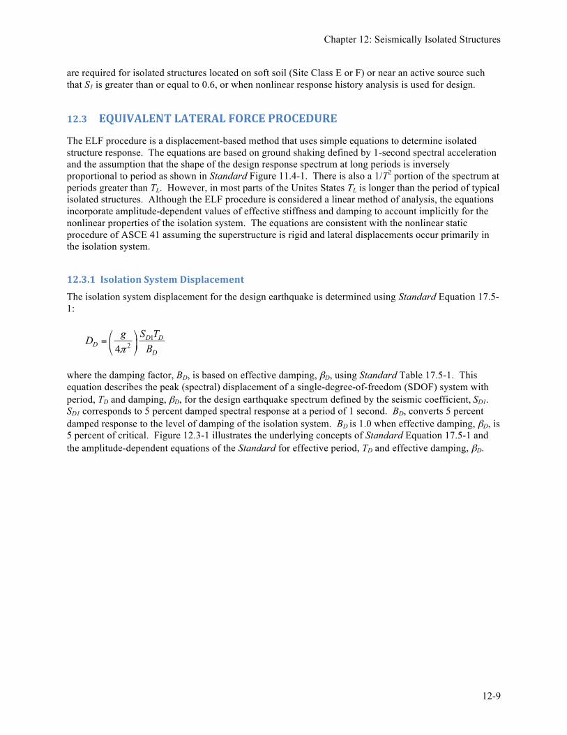
The ELF procedure is a displacement-based method that uses simple equations to determine isolated structure response. The equations are based on ground shaking defined by 1-second spectral acceleration and the assumption that the shape of the design response spectrum at long periods is inversely proportional to period as shown in Standard Figure 11.4-1. There is also a 1/T2 portion of the spectrum at periods greater than TL. However, in most parts of the Unites States TL is longer than the period of typical isolated structures. Although the ELF procedure is considered a linear method of analysis, the equations incorporate amplitude-dependent values of effective stiffness and damping to account implicitly for the nonlinear properties of the isolation system. The equations are consistent with the nonlinear static procedure of ASCE 41 assuming the superstructure is rigid and lateral displacements occur primarily in the isolation system.
12.3.1 Isolation System Displacement
The isolation system displacement for the design earthquake is determined using Standard Equation 17.5-1:
124
D DD
D
S TgDBπ
⎛ ⎞= ⎜ ⎟⎝ ⎠
where the damping factor, BD, is based on effective damping, βD, using Standard Table 17.5-1. This equation describes the peak (spectral) displacement of a single-degree-of-freedom (SDOF) system with period, TD and damping, βD, for the design earthquake spectrum defined by the seismic coefficient, SD1. SD1 corresponds to 5 percent damped spectral response at a period of 1 second. BD, converts 5 percent damped response to the level of damping of the isolation system. BD is 1.0 when effective damping, βD, is 5 percent of critical. Figure 12.3-1 illustrates the underlying concepts of Standard Equation 17.5-1 and the amplitude-dependent equations of the Standard for effective period, TD and effective damping, βD.

FEMA P-751, NEHRP Recommended Provisions: Design Examples
12-10
Figure 12.3-1 Isolation system capacity and earthquake demand The equations for maximum displacement, DM and design displacement, DD, reflect differences due to the corresponding levels of ground shaking. The maximum displacement is associated with MCER ground motions (characterized by SM1) whereas the design displacement corresponds to design earthquake ground motions (characterized by SD1). In general, the effective period and the damping factor (TM and BM, respectively) used to calculate the maximum displacement are different from those used to calculate the design displacement (TD and BD) because the effective period tends to shift and effective damping may change with the increase in the level of ground shaking. As shown in Figure 12.3-1, the calculation of effective period, TD, is based on the minimum effective stiffness of the isolation system, kDmin, as determined by prototype testing of individual isolator units. Similarly, the calculation of effective damping is based on the minimum loop area, ED, as determined by prototype testing. Use of minimum effective stiffness and damping produces larger estimates of effective period and peak displacement of the isolation system. The design displacement, DD and maximum displacement, DM, represent peak earthquake displacements at the center of mass of the building without the additional displacement that can occur at other locations due to actual or accidental mass eccentricity. Equations for determining total displacement, including the effects of mass eccentricity as an increase in the displacement at the center of mass, are based on the plan dimensions of the building and the underlying assumption that building mass and isolation stiffness have a similar distribution in plan. The increase in displacement at corners for 5 percent mass eccentricity is approximately 15 percent if the building is square in plan and as much as 30 percent if the building is long in plan. Figure 12.3-2 illustrates design displacement, DD and maximum displacement, DM, at the center of mass of the building and total maximum displacement, DTM, at the corners of an isolated building.
Mass ×Design earthquake spectral acceleration(W/g × SD1/T)
Mas
s ×Sp
ectra
l ac
cele
ratio
n
Spectral displacement
Maximum stiffness
curve
Minimum stiffness curve
Response reduction, BD(effective damping,βD > 5% of critical)
Dmaxk
Dmink
24 D1 Dg S Tπ
⎛ ⎞⎜ ⎟⎝ ⎠
2DDmin
WTk g
π=
212
DD
Dmax D
Ek D
βπ
⎛ ⎞= ⎜ ⎟⎜ ⎟
⎝ ⎠
∑
DE∑DD
bV

Chapter 12: Seismically Isolated Structures
12-11
Figure 12.3-2 Design, maximum and total maximum displacement
12.3.2 Design Forces
Forces required by the Standard for design of isolated structures are different for design of the superstructure and design of the isolation system and other elements of the structure below the isolation system (i.e., the foundation). In both cases, however, use of the maximum effective stiffness of the isolation system is required to determine a conservative value of design force. In order to provide appropriate overstrength, peak design earthquake response (without reduction) is used directly for design of the isolation system and the structure below. Design for unreduced design earthquake forces is considered sufficient to avoid inelastic response or failure of connections and other elements for ground shaking as strong as that associated with the MCER (i.e., shaking as much as 1.5 times that of the design earthquake). The design earthquake base shear, Vb, is given by Standard Equation 17.5-7: Vb = kDmaxDD where kDmax is the maximum effective stiffness of the isolation system at the design displacement, DD. Because the design displacement is conservatively based on minimum effective stiffness, Standard Equation 17.5-7 implicitly induces an additional conservatism of a worst-case combination mixing maximum and minimum effective stiffness in the same equation. Rigorous modeling of the isolation
Total Maximum Displacement(maximum considered earthquake
corner of building)Maximum Displacement
(maximum considered earthquake center of building)
Design Displacement(design earthquake center
of building)
TMD
MD
DD

FEMA P-751, NEHRP Recommended Provisions: Design Examples
12-12
system for dynamic analyses precludes mixing of maximum and minimum stiffness in the same analysis (although separate analyses typically are required to determine bounding values of both displacement and force). Design earthquake response is reduced by a modest factor for design of the superstructure above the isolation interface, as given by Standard Equation 17.5-8:
The reduction factor, RI, is defined as three-eighths of the R factor for the seismic force-resisting system of the superstructure, as specified in Standard Table 12.2-1, with an upper-bound value of 2.0. A relatively small RI factor is intended to keep the superstructure essentially elastic for the design earthquake (i.e., keeping earthquake forces at or below the true strength of the seismic force-resisting system). The Standard also imposes three limits on design forces that require the value of Vs to be at least as large as each of the following:
1. The shear force required for design of a conventional, fixed-base structure of the same effective seismic weight (and seismic force-resisting system) and period TD.
2. The shear force required for wind design.
3. A factor of 1.5 times the shear force required for activation of the isolation system.
The first two limits seldom govern design but do reflect principles of good design. The third often governs design of very long period systems with substantial effective damping (e.g., the example EOC in Sec. 12.5) and is included in the Standard to ensure that the isolation system displaces significantly before lateral forces reach the strength of the seismic force-resisting system. For designs using the ELF procedure, the lateral forces, Fx, must be distributed to each story over the height of the structure, assuming an inverted triangular pattern of lateral load (Standard Eq. 17.5-9):
Because the lateral displacement of the isolated structure is dominated by isolation system displacement, the actual pattern of lateral force in the isolated mode of response is distributed almost uniformly over height. Nevertheless, the Standard requires an inverted triangular pattern of lateral load to capture possible higher-mode effects that might be missed by not modeling superstructure flexibility and explicitly considering isolation system nonlinearity. Response history analysis that models superstructure flexibility and nonlinear properties of isolators would directly incorporate higher mode effects in the results. The ELF formulas may be used to construct plots of design displacement and base shear as a function of effective period, TD or TM, of the isolation system. For example, design displacement (DD), total maximum displacement (DTM) and design forces for the isolation system (Vb) and the superstructure (Vs) are shown in Figure 12.3-3 for a steel special concentrically braced frame (SCBF) superstructure and in
maxb D Ds
I I
V k DVR R
= =
s x xx n
i ii n
V w hFw h
=
=
∑

Chapter 12: Seismically Isolated Structures
12-13
Figure 12.3-4 for a steel ordinary concentrically braced frame (OCBF) superstructure as functions of the effective period of the isolation system.
Figure 12.3-3 Isolation system displacement and shear force (SCBF) (R/I = 6.0/1.5, RI = 2.0) (1.0 in. = 25.4 mm)
Figure 12.3-4 Isolation system displacement and shear force (OCBF) (R/I = 3.25/1.5, RI = 1.0) (1.0 in. = 25.4 mm)
Vb
VsDD
DM
DTM
0
10
20
30
40
50
0.0
0.1
0.2
0.3
0.4
0.5
1.0 1.5 2.0 2.5 3.0 3.5 4.0
Isolation system displacement (in.)
Normalized design shear, V/W
Effective period (s)
Vb, Vs
DD
DM
DTM
0
10
20
30
40
50
0.0
0.1
0.2
0.3
0.4
0.5
1.0 1.5 2.0 2.5 3.0 3.5 4.0
Isolation system displacement (in.)
Normalized design shear, V/W
Effective period (s)

FEMA P-751, NEHRP Recommended Provisions: Design Examples
12-14
Figures 12.3-3 and 12.3-4 illustrate design properties for a building located in a region of high seismicity, relatively close to an active fault, with a 1-second spectral acceleration parameter, S1, equal to 0.75 and site conditions corresponding to the C-D boundary (Site Class CD). Note: Seismic hazard and site conditions (and effective damping of the isolation system) were selected to be the same as those of the example EOC facility (Sec. 12.5). Table 12.3-1 summarizes the key response and design parameters that are used with various ELF formulas to construct the plots shown Figures 12.3-3 and 12.3-4.
Table 12.3-1 Summary of Key Response and Design Parameters Used to Construct Illustrative Plots of Design Displacements and Forces as a Function of Effective Period in Figures 12.3-3 and 12.3-4
Key Response or Design Parameter Symbol Description Value
Ground Motion and Site Amplification Parameters S1 1-Second Spectral Acceleration (g) 0.75 Ss Short Period Spectral Acceleration (g) 1.25 Fv 1-Second Site Coefficient (Site Class C-D) 1.4 Fa Short-Period Site Coefficient (Site Class C-D) 1.0
Isolation System Design Parameters βD Effective Damping - Design Level Response 20% BD Damping Factor - Design Level Response 1.5 βM Effective Damping - MCER Level Response 13% BM Damping Factor - MCER Level Response 1.3 DTM/DM Torsional Response Amplification 1.1
Superstructure Design Parameters SCBF OCBF R Response Modification Factor - Fixed-Base Structure 6.0 3.25 I Importance Factor - Fixed-Base Structure 1.5 1.5 RI Response Modification Factor - Isolated Structure 2.0 1.0 I Importance Factor - Isolated Structure 1.0 1.0 * Chapter 17 of the Standard does not require use of occupancy importance factor to determine design
loads on the superstructure of an isolated building (I = 1.0). The plots in Figures 12.3-3 and 12.3-4 illustrate the fundamental trade-off between displacement and force as a function of isolation system displacement. As the period is increased, design forces decrease and design displacements increase linearly. Plots like those shown in Figures 12.3-3 and 12.3-4 can be constructed during conceptual design once site seismicity and soil conditions are known (or are assumed) to investigate trial values of effective stiffness and damping of the isolation system. In this particular example, an isolation system with an effective period of approximately 3.5 to 4.0 seconds would require approximately 30 inches of total maximum displacement capacity, which is near the practical limit of moat covers, flexible utility connections, etc., that must accommodate isolation system displacement. Design force, Vs, on the superstructure would be approximately 10 percent of the building weight for a steel SCBF system and approximately 17 percent for a steel OCBF superstructure (subject to other limits on Vs per Standard Section 17.5.4.3).

Chapter 12: Seismically Isolated Structures
12-15
The Standard does not permit use of steel OCBFs as the superstructure of an isolated building that is an Essential Facility located in a region of high seismicity (close to an active fault). In contrast, Section 1613.6.2 of the 2006 International Building Code (IBC) permits steel OCBFs and ordinary moment frames (OMFs) to be used for structures assigned to Seismic Design Category D, E or F, provided that the following conditions are satisfied:
§ The value of RI is taken as 1.0
§ Steel OMFs and OCBFs are designed in accordance with AISC 341. The underlying concept of Section 1613.6.2 of the 2006 IBC is to trade the higher strength of steel OCBFs designed using RI = 1.0 for the larger inelastic response capacity of steel SCBFs. This trade-off is not unreasonable provided that the isolation system and surrounding structure are configured to not restrict displacement of the isolated structure in a manner that could cause large inelastic demands to occur in the superstructure. If an isolated building is designed with a superstructure system not permitted by the Standard (e.g., steel OCBFs), then the stability of the superstructure should be verified for MCER ground motions using the response history procedure with explicit modeling of the stiffening effects of isolators at very large displacements (e.g., due to high rubber strains in an elastomeric bearing, or engagement of the articulated slider with the concave plates of a friction pendulum bearing) and the effects of nearby structures (e.g., possible impact with moat walls).
12.4 DYNAMIC LATERAL RESPONSE PROCEDURE
While the ELF procedure equations are useful tools for preliminary design of the isolations system, the Standard requires a dynamic analysis for most isolated structures. Even where not strictly required by the Standard, the use of dynamic analysis (usually response history analysis) to verify the design is common.
12.4.1 Minimum Design Criteria
The Standard encourages the use of dynamic analysis but recognizes that along with the benefits of more complex models and analyses also comes an increased chance of design error. To avoid possible under-design, the Standard establishes lower-bound limits on results of dynamic analysis used for design. The limits distinguish between response spectrum analysis (a linear, dynamic method) and response history analysis (a nonlinear, dynamic method). In all cases, the lower-bound limit on dynamic analysis is established as a percentage of the corresponding design parameter calculated using the ELF procedure equations. Table 12.4-1 summarizes the percentages that define lower-bound limits on dynamic analysis. Table 12.4-1 Summary of Minimum Design Criteria for Dynamic Analysis Design Parameter Response
Spectrum Procedure
Response History
Procedure Total design displacement, DTD 90% DTD 90% DTD Total maximum displacement, DTM 80% DTM 80% DTM Design force on isolation system, Vb 90% Vb 90% Vb Design force on irregular superstructure, Vs 100% Vs 80% Vs Design force on regular superstructure, Vs 80% Vs 60% Vs

FEMA P-751, NEHRP Recommended Provisions: Design Examples
12-16
The Standard permits more liberal drift limits where the design of the superstructure is based on dynamic analysis. The ELF procedure drift limits of 0.010hsx are increased to 0.015hsx for response spectrum analysis and to 0.020hsx for response history analysis (where hsx is the story height at level x). Usually a stiff system (e.g., braced frames) is selected for the superstructure (to limit damage to nonstructural components sensitive to drift) and drift demand typically is less than approximately 0.005hsx. Standard Section 17.6.4.4 requires an explicit check of superstructure stability at the MCER displacement if the design earthquake story drift ratio exceeds 0.010/RI.
12.4.2 Modeling Requirements
As for the ELF procedure, the Standard requires the isolation system to be modeled for dynamic analysis using stiffness and damping properties that are based on tests of prototype isolator units. Additionally, dynamic analysis models are required to account for the following:
§ Spatial distribution of individual isolator units.
§ Effects of actual and accidental mass eccentricity.
§ Overturning forces and uplift of individual isolator units.
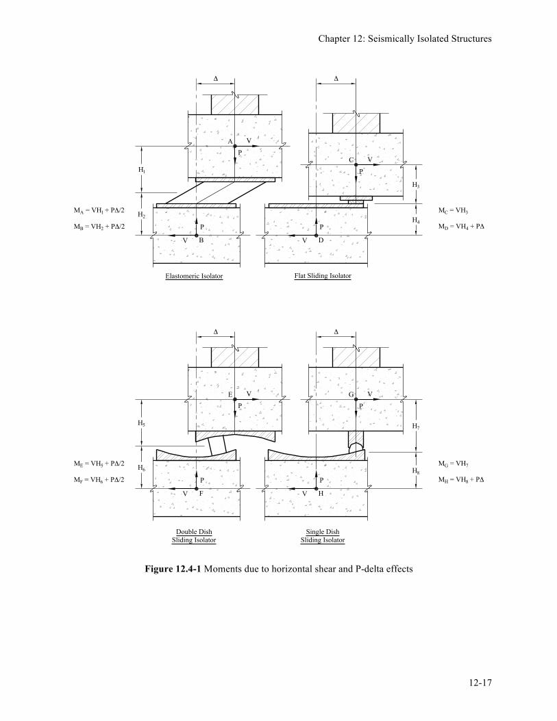
§ Variability of isolation system properties (due to rate of loading, etc.). The Standard requires explicit nonlinear modeling of elements if response history analysis is used to justify design loads less than those permitted for ELF or response spectrum analysis. This option is seldom exercised and the superstructure typically is modeled using linear elements and conventional methods. Special modeling concerns for isolated structures include two important and related issues: uplift of isolator units and P-delta effects on the isolated structure. Typically, isolator units have little or no ability to resist tension forces and can uplift when earthquake overturning (upward) loads exceed factored gravity (downward) loads. Local uplift of individual elements is permitted (Standard Sec. 17.2.4.7), provided the resulting deflections do not cause overstress or instability of the isolated structure. To calculate uplift effects, gap elements may be used in nonlinear models or tension may be released manually in linear models. The effects of P-delta loads on the isolation system and adjacent elements of the structure can be quite significant. The compression load, P, can be large due to earthquake overturning (and factored gravity loads) at the same time that large displacements occur in the isolation system. Computer analysis programs (most of which are based on small-displacement theory) may not correctly calculate P-delta moments at the isolator level in the structure above or in the foundation below. Figure 12.4-1 illustrates moments due to P-delta effects (and horizontal shear loads) for an elastomeric bearing isolation system and three configurations of a sliding isolation system. For the elastomeric system, the P-delta moment is split one-half up and one-half down. For the flat and single-dish sliding systems, the full P-delta moment is applied to the foundation below (due to the orientation of the sliding surface). A reverse (upside down) orientation of the flat and single-sided sliding systems would apply the full P-delta moment on the structure above. For the double-dish sliding system, P-delta moments are split one-half up and one-half down, in a manner similar to an elastomeric bearing, provided that the friction (and curvature) properties of the top and bottom concave dishes are the same.
Chapter 12: Seismically Isolated Structures
12-17
Figure 12.4-1 Moments due to horizontal shear and P-delta effects
C
A
B D
Elastomeric Isolator Flat Sliding Isolator
V
P
V
P
P
V
V
P
E
F
Double DishSliding Isolator
Single DishSliding Isolator
V
P
V
PG
HV
P
P
V
Δ Δ
H1
H2 H4
H3
Δ Δ
H5
H6 H8
H7
M A = VH
1 + PΔ/2
M B = VH
2 + PΔ/2
M C = VH
3
M D = VH
4 + PΔ
M E = VH
5 + PΔ/2
M F = VH
6 + PΔ/2
M G = VH
7
M H = VH
8 + PΔ

FEMA P-751, NEHRP Recommended Provisions: Design Examples
12-18
12.4.3 Response Spectrum Analysis
Response spectrum analysis methods require that isolator units be modeled using amplitude-dependent values of effective stiffness and damping that are essentially the same as those of the ELF procedure, subject to the limitation that the effective damping of the isolated modes of response not exceed 30 percent of critical. Higher modes of response usually are assumed to have 2 to 5 percent damping, a value of damping appropriate for a superstructure that remains essentially elastic. As previously noted, maximum and minimum values of effective stiffness of the isolation system are used to calculate separately maximum displacement of the isolation system (using minimum effective stiffness) and maximum forces in the superstructure (using maximum effective stiffness). The Standard requires horizontal loads to be applied in two orthogonal directions and peak response of the isolation system and other structural elements is determined using the 100 percent plus 30 percent combination method. The Provisions now define ground motions in terms of maximum spectral response in the horizontal plane (where previous editions used average horizontal response). Consequently, at a given period of interest (for instance, the effective period of the isolation system), it may be overly conservative to combine 30 percent of the maximum spectral response load applied in the orthogonal direction with 100 percent of the maximum spectral response load applied in the horizontal direction of interest to determine peak spectral response of the isolation system and other structural elements. In the opinion of the author, it would be reasonable to not apply 30 percent of spectral response load at the fundamental (isolated) mode in the orthogonal direction when applying 100 percent of the maximum spectral response load in the horizontal direction of interest. However, the 100 percent plus 30 percent combination method would still be appropriate for all higher modes, since spectral response at higher-mode periods is, in general, independent of fundamental (isolated) mode spectral response. The design shear at any story, determined by RSA, cannot be taken as less than the story shear resulting from application of the ELF distribution of force over height (Standard Equation 17.5-9) where anchored to a value of base shear, Vs, determined by RSA in the direction of interest. This limit is intended to avoid underestimation of higher-mode response when isolators are modeled using effective stiffness and damping properties, rather than actual nonlinear properties. The value of Vs determined by RSA is typically less than the value of Vs prescribed by ELF using Standard Equation 17.5-8, which combines maximum effective stiffness, kDmax, with design displacement, DD, based on minimum effective stiffness, although the difference generally is small and the values of design shear determined by RSA are similar to those required by the ELF procedure. Standard Section 17.6.3.4 does not explicitly require the value of base shear, Vs, determined by RSA to comply with the Standard Section 17.5.4.2 limits on Vs. In the opinion of the author, the Standard Section 17.5.4.3 limits on base shear apply to all methods of analysis and should be complied with when RSA is used as the basis for design. It may be noted that Standard Section 17.6.4.2 requires Vs to comply with the Standard Section 17.5.4.3 limits on Vs when the design is based on the response history analysis procedure, which otherwise has more liberal design shear requirements than either the RSA or ELF procedure. As previously discussed (Sec. 12.3.2), the third limit of Standard Section 17.5.4.3 is included in the Standard to ensure that the isolation system displaces significantly before lateral forces reach the strength of the seismic force-resisting system.
12.4.4 Response History Analysis
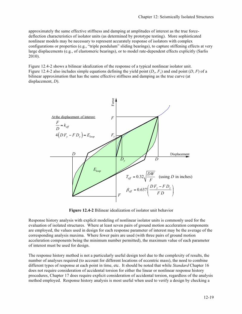
For response history analysis, nonlinear force-deflection characteristics of isolator units are modeled explicitly (rather than using effective stiffness and damping). For most types of isolators, force-deflection properties can be approximated by bilinear, hysteretic curves that can be modeled using commercially available nonlinear structural analysis programs. Such bilinear hysteretic curves should have
Chapter 12: Seismically Isolated Structures
12-19
approximately the same effective stiffness and damping at amplitudes of interest as the true force-deflection characteristics of isolator units (as determined by prototype testing). More sophisticated nonlinear models may be necessary to represent accurately response of isolators with complex configurations or properties (e.g., “triple pendulum” sliding bearings), to capture stiffening effects at very large displacements (e.g., of elastomeric bearings), or to model rate-dependent effects explicitly (Sarlis 2010). Figure 12.4-2 shows a bilinear idealization of the response of a typical nonlinear isolator unit. Figure 12.4-2 also includes simple equations defining the yield point (Dy, Fy) and end point (D, F) of a bilinear approximation that has the same effective stiffness and damping as the true curve (at displacement, D).
Figure 12.4-2 Bilinear idealization of isolator unit behavior Response history analysis with explicit modeling of nonlinear isolator units is commonly used for the evaluation of isolated structures. Where at least seven pairs of ground motion acceleration components are employed, the values used in design for each response parameter of interest may be the average of the corresponding analysis maxima. Where fewer pairs are used (with three pairs of ground motion acceleration components being the minimum number permitted), the maximum value of each parameter of interest must be used for design. The response history method is not a particularly useful design tool due to the complexity of results, the number of analyses required (to account for different locations of eccentric mass), the need to combine different types of response at each point in time, etc. It should be noted that while Standard Chapter 16 does not require consideration of accidental torsion for either the linear or nonlinear response history procedures, Chapter 17 does require explicit consideration of accidental torsion, regardless of the analysis method employed. Response history analysis is most useful when used to verify a design by checking a
Forc
e
Displacement
loopE
F
F
DD
( )4
eff
y y loop
F kDDF F D E
≈
− ≈
0.32 (using in inches)
0.637
eff
y yeff
DWT DFDF F D
F Dβ
=
−⎛ ⎞= ⎜ ⎟
⎝ ⎠
At the displacement of interest:
yD
yF
FEMA P-751, NEHRP Recommended Provisions: Design Examples
12-20
few key design parameters, such as isolation displacement, overturning loads and uplift and story shear force. The Provisions (Sections 17.3.2 and 16.1.3.2) now require ground motions to be scaled to match maximum spectral response in the horizontal plane (where previous editions defined spectral response in terms of average horizontal response). In concept, at a given period of interest, maximum spectral response of scaled records should, on average, be the same as that defined by the design spectrum of interest (DE or MCER). Neither the Standard nor the Provisions specify how the two scaled components of each record should be applied to a three-dimensional model (i.e., how the two components of each record should be oriented with respect to the axes of the model). This lack of guidance has sometimes caused users to perform an unnecessarily large number of response history analyses for design verification of an isolated structure. In the author’s opinion, the following steps describe an acceptable approach for scaling, orienting and applying ground motion components to a three-dimensional model of an isolated structure (when based on the new maximum definition of the ground motions).
§ Step 1 - Selection and Scaling of Records. Select and scale ground motion records as required by Provisions Section 17.3.2. The records would necessarily be scaled differently to match the DE spectrum and the MCER spectrum, respectively. While the Provisions permits as few as three records for response history analysis (with design/verification based the most critical of the three), a set of at least seven records is recommended such that the average value of the response parameter of interest may be used for design or design verification.
§ Step 2 - Grouping of Stronger Components. Group the horizontal components of each record in
terms of stronger and weaker components. The stronger component of each record is the component that has the larger spectral response at periods of interest. For isolated structures, periods of interest are approximately from TD to TM. The records may require rotation of horizontal axes before grouping to better distinguish between stronger and weaker components at the period of interest. Orient stronger horizontal components such that peak response occurs in the same (positive or negative) direction. In general, the same grouping of components can be used for both DE and MCER analyses (just scaled by a different factor), since TD and TM are typically about the same and response spectra do not vary greatly from period to period at long periods.
§ Step 3 - Verification of Component Grouping. Verify that the average spectral response of the set
of stronger components is comparable to the design spectrum of interest (e.g., DE or MCER spectrum) at periods of interest (i.e., TM, if checking MCER displacement). If the average spectrum of stronger components is not adequate, then the scaling factor should be increased accordingly. Note: Increasing ground motions to match average spectral response of stronger components with the design spectrum of interest is not required by Provisions Section 17.3.2 but is consistent with the “maximum” definition of ground motions.
§ Step 4 - Application of Scaled Records. In general, apply the set of scaled records to the three-
dimensional model of the isolated structure in four basic orientations with respect to the primary (orthogonal) horizontal axes of the superstructure:
1. Apply the set of scaled records with stronger components aligned in the positive direction of
the first horizontal axis of the model.

Chapter 12: Seismically Isolated Structures
12-21
2. Apply the set of scaled records with stronger components aligned in the positive direction of the second horizontal axis of the model.
3. Apply the set of scaled records with stronger components aligned in the negative direction of
the first horizontal axis of the model.
4. Apply the set of scaled records with stronger components aligned in the negative direction of the second horizontal axis of the model.
For each of the four sets of analyses, find the average value of the response parameter of interest (if the set of ground motion contains at least seven records) or the maximum value of the response parameter (if the set of ground motions contains less than seven records). The more critical response of the four sets of analyses should be used for design or design verification.
The four orientations of ground motions of Step 4 are required, in general, for design of elements, since the most critical positive or negative direction of peak response typically is not known for individual elements. However, for design verification of key global response parameters that are relatively insensitive to positive/negative orientation of ground motion components (e.g., maximum isolation system displacement, peak story shear, peak story displacement), only the first two sets of analyses are necessary. Although the above steps require some “homework” by the engineer to develop an appropriate set of scaled records, only two sets of response history analyses are typically required to verify the design of most isolated structures. The above response history analysis recommendations apply to each model of the structure, which necessarily include at least two models whose properties represent upper-bound and lower-bound force-deflection properties of the isolation system, respectively. Different models could also be used to explicitly evaluate various locations of accidental mass eccentricity, as required by Standard Section 17.6.2.1.b. However, this approach would require multiple additional models to consider “the most disadvantageous location of accidental eccentric mass.” In the opinion of the author, these additional response history analyses are unnecessary and the effects of accidental mass eccentricity can be calculated by factoring the results of response history analyses (of a model that does not explicitly include accidental mass eccentricity). The amount by which the response parameter of interest should be factored may be determined by assuming that accidental torsion increases response in proportion to the increase in isolation system displacement, as prescribed by the ELF requirements of Standard Section 17.5.3.5.
12.5 EMERGENCY OPERATIONS CENTER USING DOUBLE-‐CONCAVE FRICTION PENDULUM BEARINGS, OAKLAND, CALIFORNIA
This example features the seismic isolation of a hypothetical EOC, assumed to be located in Oakland, California, approximately 6 kilometers from the Hayward fault. The isolation system incorporates double-concave friction pendulum sliding bearings, although other types of isolators could have been used in this example. Isolation is an appropriate design strategy for EOCs and other buildings where the goal is to limit earthquake damage and protect facility function. The example illustrates the following design topics:
§ Determination of seismic design parameters.
§ Preliminary design of superstructure and isolation systems (using the ELF procedure).
§ Dynamic analysis of a seismically isolated structure.

FEMA P-751, NEHRP Recommended Provisions: Design Examples
12-22
§ Specification of isolation system design and testing criteria.
While the example includes development of the entire structural system, the primary focus is on the design and analysis of the isolation system. Examples in other chapters have more in-depth descriptions of the provisions governing detailed design of the superstructure above and the foundation below.
12.5.1 System Description
This EOC is a three-story, steel-braced frame structure with a large, centrally located mechanical penthouse. Story heights are 14 feet at the first floor to accommodate computer access flooring and other architectural and mechanical systems and 12 feet at the second and third floors (and penthouse). The roof and penthouse roof decks are designed for significant live load to accommodate a helicopter landing pad and to meet other functional requirements of the EOC. Figure 12.5-1 shows the three-dimensional model of the structural system.
Figure 12.5-1 Three-dimensional model of the structural system The structure (which is regular in configuration) has plan dimensions of 100 feet by 150 feet at all floors except for the penthouse, which is approximately 50 feet by 100 feet in plan. Columns are spaced at 25 feet in both directions. Figures 12.5-2 and 12.5-3 are framing plans for the typical floor levels (1, 2, 3 and roof) and the penthouse roof.

Chapter 12: Seismically Isolated Structures
12-23
Figure 12.5-2 Typical floor framing plan (1.0 ft = 0.3048 m)
Figure 12.5-3 Penthouse roof framing plan (1.0 ft = 0.3048 m) The vertical load-carrying system consists of concrete fill on steel deck floors, supported by steel beams at 8.3 feet on center and steel girders at column lines. Isolator units support the columns below the first floor. The foundation is a heavy mat (although spread footings or piles could be used depending on the soil type, depth to the water table and other site conditions).
A
B
C
D
E
25'-0"
25'-0"
25'-0"
25'-0"
25'-0"25'-0"25'-0"25'-0" 25'-0" 25'-0"
1 2 43 5 6 7
X
Y
25'-0"
25'-0"
25'-0"
25'-0"
25'-0"25'-0"25'-0"25'-0" 25'-0" 25'-0"A
B
C
D
E
1 2 43 5 6 7
X
Y

FEMA P-751, NEHRP Recommended Provisions: Design Examples
12-24
The lateral system consists of a roughly symmetrical pattern of concentrically braced frames. These frames are located on Column Lines B and D in the longitudinal direction and on Column Lines 2, 4 and 6 in the transverse direction. Figures 12.5-4 and 12.5-5 show the longitudinal and transverse elevations, respectively. Braces are specifically configured to reduce the concentration of earthquake overturning and uplift loads on isolator units by:
§ Increasing the number of bays with bracing at lower stories.
§ Locating braces at interior (rather than perimeter) column lines (providing more hold-down weight).
§ Avoiding common end columns for transverse and longitudinal bays with braces.
Figure 12.5-4 Longitudinal bracing elevation (Column Lines B and D)
1
Penthouse Roof
Roof
Third Floor
Second Floor
First FloorBase
6 bays at 25'-0" = 150'-0"
Lines B and D
2 3 4 65 7

Chapter 12: Seismically Isolated Structures
12-25
Figure 12.5-5 Transverse bracing elevations: (a) on Column Lines 2 and 6 and (b) on Column Line 4
The isolation system has 35 identical elastomeric isolator units, located below columns. The first floor is just above grade and the isolator units are approximately 3 feet below grade to provide clearance below the first floor for construction and maintenance personnel. A short retaining wall borders the perimeter of the facility and provides approximately 3 feet of “moat” clearance for lateral displacement of the isolated structure. Access to the EOC is provided at the entrances by segments of the first floor slab, which cantilever over the moat. Girders at the first-floor column lines are much heavier than the girders at other floor levels and have moment-resisting connections to columns. These girders stabilize the isolator units by resisting moments due to vertical (P-delta effect) and horizontal (shear) loads. Column extensions from the first floor to the top plates of the isolator units are stiffened in both horizontal directions, to resist these moments and to serve as stabilizing haunches for the beam-column moment connections.
12.5.2 Basic Requirements
12.5.2.1 Specifications.
§ General: ASCE Standard ASCE 7-05 (Standard)
§ Seismic Loads: 2009 NEHRP Recommended Provisions (Provisions)
§ Other Loads and Load Combinations: 2006 International Building Code (2006 IBC) 12.5.2.2 Materials.
§ Concrete: Strength (floor slabs): f ‘c = 3 ksi
Penthouse Roof
Roof
Third Floor
Second Floor
First FloorBase
E D C B A
4 bays at 25'-0" = 100'-0" 4 bays at 25'-0" = 100'-0"
(b) Line 4(a) Lines 2 and 6
E D C B A
FEMA P-751, NEHRP Recommended Provisions: Design Examples
12-26
Strength (foundations below isolators): f ‘c = 5 ksi Weight (normal): 150 pcf
§ Steel: Columns: Fy = 50 ksi Primary first-floor girders (at column lines): Fy = 50 ksi Other girders and floor beams: Fy = 36 ksi Braces: Fy = 46 ksi
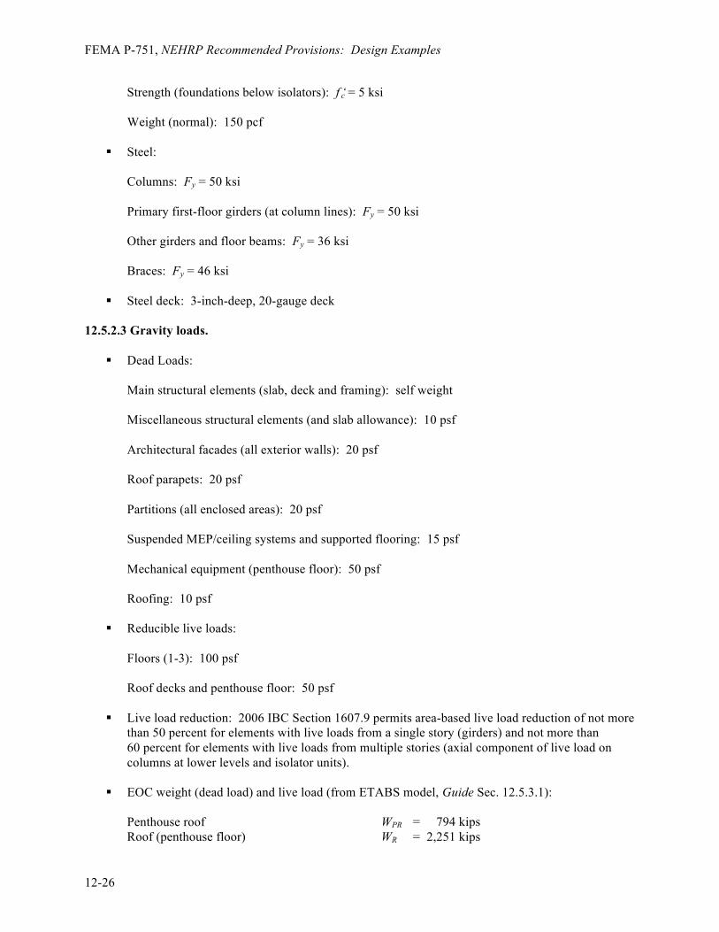
§ Steel deck: 3-inch-deep, 20-gauge deck 12.5.2.3 Gravity loads.
§ Dead Loads: Main structural elements (slab, deck and framing): self weight Miscellaneous structural elements (and slab allowance): 10 psf Architectural facades (all exterior walls): 20 psf Roof parapets: 20 psf Partitions (all enclosed areas): 20 psf Suspended MEP/ceiling systems and supported flooring: 15 psf Mechanical equipment (penthouse floor): 50 psf Roofing: 10 psf
§ Reducible live loads: Floors (1-3): 100 psf Roof decks and penthouse floor: 50 psf
§ Live load reduction: 2006 IBC Section 1607.9 permits area-based live load reduction of not more than 50 percent for elements with live loads from a single story (girders) and not more than 60 percent for elements with live loads from multiple stories (axial component of live load on columns at lower levels and isolator units).
§ EOC weight (dead load) and live load (from ETABS model, Guide Sec. 12.5.3.1):
Penthouse roof WPR = 794 kips Roof (penthouse floor) WR = 2,251 kips
Chapter 12: Seismically Isolated Structures
12-27
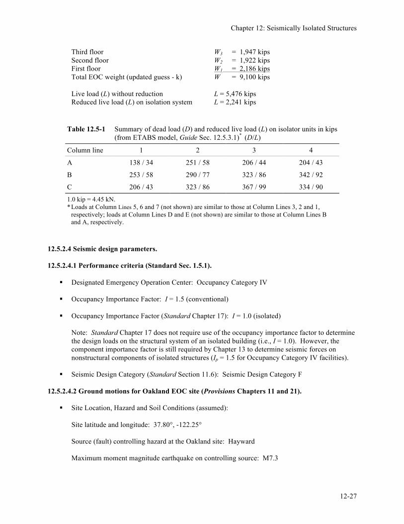
Third floor W3 = 1,947 kips Second floor W2 = 1,922 kips First floor W1 = 2,186 kips Total EOC weight (updated guess - k) W = 9,100 kips
Live load (L) without reduction L = 5,476 kips Reduced live load (L) on isolation system L = 2,241 kips
Table 12.5-1 Summary of dead load (D) and reduced live load (L) on isolator units in kips (from ETABS model, Guide Sec. 12.5.3.1)* (D/L)
Column line 1 2 3 4
A 138 / 34 251 / 58 206 / 44 204 / 43
B 253 / 58 290 / 77 323 / 86 342 / 92
C 206 / 43 323 / 86 367 / 99 334 / 90
1.0 kip = 4.45 kN. * Loads at Column Lines 5, 6 and 7 (not shown) are similar to those at Column Lines 3, 2 and 1,
respectively; loads at Column Lines D and E (not shown) are similar to those at Column Lines B and A, respectively.
12.5.2.4 Seismic design parameters. 12.5.2.4.1 Performance criteria (Standard Sec. 1.5.1).
§ Designated Emergency Operation Center: Occupancy Category IV
§ Occupancy Importance Factor: I = 1.5 (conventional)
§ Occupancy Importance Factor (Standard Chapter 17): I = 1.0 (isolated) Note: Standard Chapter 17 does not require use of the occupancy importance factor to determine the design loads on the structural system of an isolated building (i.e., I = 1.0). However, the component importance factor is still required by Chapter 13 to determine seismic forces on nonstructural components of isolated structures (Ip = 1.5 for Occupancy Category IV facilities).
§ Seismic Design Category (Standard Section 11.6): Seismic Design Category F 12.5.2.4.2 Ground motions for Oakland EOC site (Provisions Chapters 11 and 21).
§ Site Location, Hazard and Soil Conditions (assumed):
Site latitude and longitude: 37.80°, -122.25° Source (fault) controlling hazard at the Oakland site: Hayward Maximum moment magnitude earthquake on controlling source: M7.3

FEMA P-751, NEHRP Recommended Provisions: Design Examples
12-28
Closest distance from site to Hayward Fault (Joyner-Boore distance): 5.9 km Site soil type (assumed for preliminary design): Site Class C-D Site shear wave velocity (assumed for response history analysis): vs,30 = 450 m/s
§ Short-Period Design Parameters (USGS web site):
Short-period MCER spectral acceleration (USGS 2009): SS = 1.24 Site coefficient (Standard Table 11.4-1): Fa = 1.0 Short-period MCER spectral acceleration adjusted for site class (FaSS): SMS = 1.24 DE spectral acceleration (2/3SMS): SDS = 0.83
§ 1-Second Design Parameters (USGS web site):
1-Second MCER spectral acceleration: S1 = 0.75 Site coefficient (Standard Table 11.4-2): Fv = 1.4 1-Second MCER spectral acceleration adjusted for site class (FvS1): SM1 = 1.05 DE spectral acceleration (2/3SM1): SD1 = 0.7
12.5.2.4.3 Design spectra (Provisions Section 11.4). Figure 12.5-6 plots DE and MCER response spectra as constructed in accordance with the procedure of Provisions Section 11.4 using the spectrum shape defined by Provisions Figure 11.4-1. Standard Section 17.3.1 requires a site-specific ground motion hazard analysis to be performed in accordance with Chapter 21 for sites with S1 greater than 0.6 (e.g., sites near active sources). Subject to other limitations of Provisions Section 21.4, the resulting site-specific DE and MCER spectra may be taken as less than 100 percent but not less than 80 percent of the default design spectrum of Standard Figure 11.4-1.

Chapter 12: Seismically Isolated Structures
12-29
Figure 12.5-6 DE and MCER spectra and 80 percent limits For this example, site-specific spectra for the design earthquake and the maximum considered earthquake were assumed to be 100 percent of the respective spectra shown in Figure 12.5-6. In general, site-specific spectra for regions of high seismicity, with well defined fault systems (like the Hayward fault), would be expected to be similar to the default design spectra of Standard Figure 11.4-1. 12.5.2.4.4 DE and MCER ground motion records (Standard Sec. 17.3.2). For response history analysis, Standard Section 17.6.3.4 requires at least three pairs of horizontal ground motion acceleration components to be selected from actual earthquake records and scaled to match either the DE or the MCER spectrum and at least seven pairs if the average value of the response parameter of interest is used for design (which is typically the case). Selection and scaling of appropriate ground motions should be performed by a ground motion expert experienced in earthquake hazard of the region, considering site conditions, earthquake magnitudes, fault distances and source mechanisms that influence ground motion hazard at the building site. For this example, a set of seven ground motion records are selected from the near-field (NF) and far-field (FF) record sets of FEMA P-695. FEMA P-695 is a convenient source of the 50 strongest ground motion records of large magnitude earthquakes available from the Pacific Earthquake Engineering Research Center (PEER) NGA database (PEER 2006), the records most suitable for response history evaluation of structures in regions of high seismicity. The seven records selected from the FEMA P-695 ground motion sets have fault source and site characteristics that best match those of the example EOC, that is, records of magnitude M7.0 or greater earthquakes recorded close to fault rupture at soil sites (Site Class C or D). Table 12.5-2 lists these seven earthquake records and summarizes key properties. As shown in this table, the average magnitude (M7.37), the average site-source distance (5.2 km) and the average shear wave
MCER
0.8MCER
DE
0.8DE
0.0
0.5
1.0
1.5
2.0
0.0 1.0 2.0 3.0 4.0 5.0
Spec
tral A
ccel
erat
ion,
Sa
(g)
Period, T (s)

FEMA P-751, NEHRP Recommended Provisions: Design Examples
12-30
velocity (446 m/s) closely match the maximum magnitude of the Hayward fault (M7.3), the closest distance from the Hayward fault to the Oakland site (5.9 km) and the Oakland site conditions (Site Class C-D), respectively, as required by record selection requirements of Standard Section 17.3.2. Table 12.5-2 Seven Earthquake Records Selected for Response History Analysis of
Example Base-Isolated EOC Facility
FEMA P-695 Record ID No.
Earthquake Source Characteristics Site Conditions
Year Name Record Station
Mag. (MW)
Distance, Df (km)
Fault Mechanis
m
Site Class
vS,30 (m/s)
JB Rupture NF-8 1992 Landers Lucerne 7.3 2.2 15.4 Strike-slip C 685 FF-10 1999 Kocaeli Arcelik 7.5 10.6 13.5 Strike-slip C 523 NF-25 1999 Kocaeli Yarimca 7.5 1.4 5.3 Strike-slip D 297 FF-3 1999 Duzce Bolu 7.1 12.0 12.0 Strike-slip D 326 NF-14 1999 Duzce Duzce 7.1 0.0 6.6 Strike-slip D 276
FF-4 1999 Hector Mine Hector 7.1 10.4 11.7 Strike-slip C 685
NF-28 2002 Denali TAPS PS#10 7.9 0.2 3.8 Strike-slip D 329
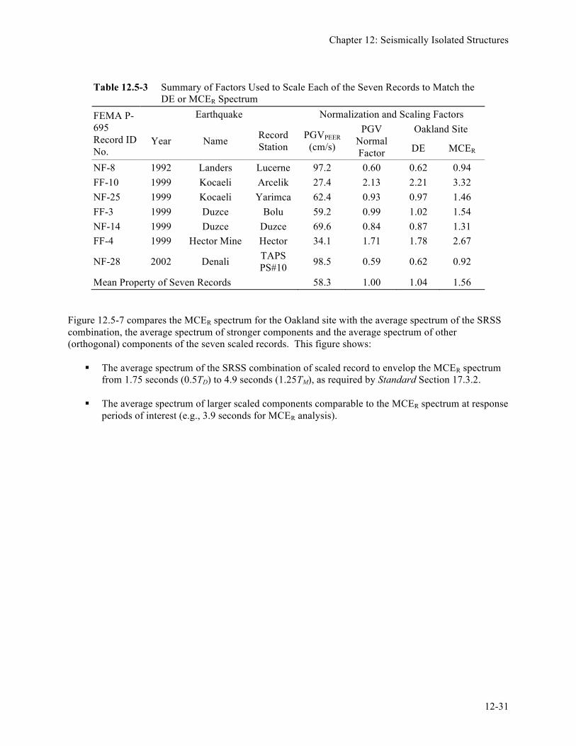
Mean Property of Seven Records 7.37 5.2 9.8 446 Standard Section 17.3.2 provides criteria for scaling earthquake records to match a target spectrum over the period range of interest, defined as 0.5TD to 1.25TM. In this example, TD and TM are 3.5 and 3.9 seconds, respectively, so the period range of interest is from 1.75 to 4.9 seconds. For each period in this range, the average of the square-root-of-the-sum-of-the-squares (SRSS) combination of each pair of horizontal components of scaled ground motion should be equal to or greater than the target spectrum. The target spectrum is defined as 1.0 times the design spectrum of interest (either the DE or the MCER spectrum). Table 12.5-3 summarizes the factors used to scale the seven records to mach either the DE or MCER spectrum, in accordance with Standard Section 17.3.2. The seven records were first “normalized” by their respective values of PGVPEER to reduce inappropriate amounts of record-to-record variability using the procedures of Section A.8 of FEMA P-695. As shown in Table 12.5-3, PGV normalization tends to increase the intensity of those records of smaller than average magnitude events or from sites farther than average from the source and to decrease the intensity of those records of larger than average magnitude events or from sites closer than average to the source, but has no net effect on the overall intensity of the record set (i.e., median value of normalization factors is 1.0 for the record set). Scaling factors were developed such that the average value of the response spectra of normalized records equals or exceeds the spectrum of interest (either the DE or MCER spectrum) over the period range of interest, 1.75 to 4.9 seconds. These scaling factors are given in Table 12.5-3 and reflect the total amount that each as-recorded ground motion is scaled for response history analysis. Table 12.5-3 shows that a median scaling factor of 1.04 is required to envelop the DE spectrum (records are increased slightly, on average, to match the DE spectrum) and a median scaling factor of 1.56 is required to envelop the MCER spectrum over the period range of interest.
Chapter 12: Seismically Isolated Structures
12-31
Table 12.5-3 Summary of Factors Used to Scale Each of the Seven Records to Match the
DE or MCER Spectrum
FEMA P-695 Record ID No.
Earthquake Normalization and Scaling Factors
Year Name Record Station
PGVPEER (cm/s)
PGV Normal Factor
Oakland Site
DE MCER
NF-8 1992 Landers Lucerne 97.2 0.60 0.62 0.94 FF-10 1999 Kocaeli Arcelik 27.4 2.13 2.21 3.32 NF-25 1999 Kocaeli Yarimca 62.4 0.93 0.97 1.46 FF-3 1999 Duzce Bolu 59.2 0.99 1.02 1.54 NF-14 1999 Duzce Duzce 69.6 0.84 0.87 1.31 FF-4 1999 Hector Mine Hector 34.1 1.71 1.78 2.67
NF-28 2002 Denali TAPS PS#10 98.5 0.59 0.62 0.92
Mean Property of Seven Records 58.3 1.00 1.04 1.56 Figure 12.5-7 compares the MCER spectrum for the Oakland site with the average spectrum of the SRSS combination, the average spectrum of stronger components and the average spectrum of other (orthogonal) components of the seven scaled records. This figure shows:
§ The average spectrum of the SRSS combination of scaled record to envelop the MCER spectrum from 1.75 seconds (0.5TD) to 4.9 seconds (1.25TM), as required by Standard Section 17.3.2.
§ The average spectrum of larger scaled components comparable to the MCER spectrum at response
periods of interest (e.g., 3.9 seconds for MCER analysis).

FEMA P-751, NEHRP Recommended Provisions: Design Examples
12-32
Figure 12.5-7 Comparison of the MCER spectrum with the average spectrum of the SRSS
combination of the seven scaled records, the average spectrum of the seven larger components of the seven scaled records and the average spectrum of the other orthogonal
components of the seven scaled records listed in Table 12.5-3 12.5.2.5 Structural design criteria. 12.5.2.5.1 Design basis.
§ Seismic force-resisting system: Special steel concentrically braced frames (height < 100 feet)
§ Response modification factor, R (Standard Table 12.2-1): R = 6 (conventional)
§ Response modification factor for design of the superstructure, RI (Standard Sec. 17.5.4.2, 3/8R ≤ 2): RI = 2 (isolated)
§ Plan irregularity (of superstructure) (Standard Table 12.3-1): None
§ Vertical irregularity (of superstructure) (Standard Table 12.3-2): None
§ Lateral response procedure (Standard Sec. 17.4.1, S1 > 0.6): Dynamic analysis
§ Redundancy factor (Standard Sec. 12.3.4): ρ ≥ 1.0 (conventional); ρ = 1.0 (isolated)
Standard Section 12.3.4 requires the use of a calculated ρ value, which could be greater than 1.0 for a conventional structure with a brace configuration similar to the superstructure of the base-isolated EOC.
Average, SRSS
MCER
0.0
0.5
1.0
1.5
2.0
0.0 1.0 2.0 3.0 4.0 5.0
Spec
tral A
ccel
erat
ion,
Sa
(g)
Period, T (s)

Chapter 12: Seismically Isolated Structures
12-33
However, in the author’s opinion, the use of RI equal to 2.0 (rather than R equal to 6) as required by Standard Section 17.5.4.2 precludes the need to further increase superstructure design forces for redundancy. 12.5.2.5.2 Horizontal earthquake loads and effects (Standard Chapters 12 and 17).
§ Design earthquake (acting in either the X or Y direction): DE (site specific)
§ Maximum considered earthquake (acting in either the X or Y direction): MCE (site specific)
§ Mass eccentricity - actual plus accidental: 0.05b = 5 ft (X direction); 0.05d = 7.5 ft (Y direction) The superstructure is essentially symmetric about both primary horizontal axes, however, the placement of the braced frames results in a ratio of maximum corner displacement to average displacement of 1.25 including accidental eccentricity, exceeding the threshold of 1.2 per the definition of the Standard. If the building were not on isolators, the accidental torsional eccentricity would need to be increased from 5 percent to 5.4 percent of the building dimension. The input to the superstructure is controlled by the isolation system and it is the author’s opinion that the amplification of accidental torsion is not necessary for such otherwise regular structures. Future editions of the Standard should address this issue. Also refer to the discussion of analytical modeling of accidental eccentricities in Guide Chapter 4.
§ Superstructure design (reduced DE response): QE = QDE/2 = DE/2.0
§ Isolation system and foundation design (unreduced DE response) : QE = QDE = DE/1.0
§ Check of isolation system stability (unreduced MCE response): QE = QMCE = MCE/1.0 12.5.2.5.3 Combination of horizontal earthquake load effects. Response due earthquake loading in the X and Y directions is as follows: QE = Max (1.0QEX+0.3QEY, 0.3QEX+1.0QEY) In general, the horizontal earthquake load effect, QE, on the response parameter of interest is influenced by only one direction of horizontal earthquake load and QE = QEX or QE = QEY. Exceptions include vertical load on isolator units due to earthquake overturning forces. 12.5.2.5.4 Combination of horizontal and vertical earthquake load effects.
§ Design earthquake (QE + 0.2SDSD): E = QE + 0.17D
§ Maximum considered earthquake (QE + 0.2SMSD): E = QE + 0.25D 12.5.2.5.5 Superstructure design load combinations (2006 IBC, Sec. 1605.2.1, using RI = 2).
§ Gravity loads (dead load and reduced live load): 1.2D + 1.6L
§ Gravity and earthquake loads (1.2D + 0.5L + 1.0E): 1.37D + 0.5L + QDE/2
§ Gravity and earthquake loads (0.9D - 1.0E): 0.73D - QDE/2 12.5.2.5.6 Isolation system and foundation design load combinations (2006 IBC, Sec. 1605.2.1).

FEMA P-751, NEHRP Recommended Provisions: Design Examples
12-34
§ Gravity loads (for example, long term load on isolator units): 1.2D + 1.6L
§ Gravity and earthquake loads (1.2D + 0.5L + 1.0E): 1.37D + 0.5L + QDE
§ Gravity and earthquake loads (0.9D - 1.0E): 0.73D - QDE
12.5.2.5.7 Isolation system stability load combinations (Standard Sec. 17.2.4.6).
§ Maximum short term load on isolator units (1.2D + 1.0L + |E|): 1.45D + 1.0L + QMCE
§ Minimum short term load on isolator units (0.8D - |E|): 0.8D - QMCE
Note that in the above combinations, the vertical earthquake load (0.2SMSD) component of |E| is included in the maximum (downward) load combination but excluded from the minimum (uplift) load combination. It is the author’s opinion that vertical earthquake ground shaking is of a dynamic nature, changing direction too rapidly to affect appreciably uplift of isolator units and need not be used with the load combinations of Standard Section 17.2.4.6 for determining minimum (uplift) vertical loads on isolator units due to the MCER.
12.5.3 Seismic Force Analysis
12.5.3.1 Basic approach to modeling. To expedite calculation of loads on isolator units and other elements of the seismic-force-resisting system, a three-dimensional model of the EOC is developed and analyzed using the ETABS computer program (CSI, 2009). While there are a number of commercially available programs to choose from, ETABS is selected for this example since it permits the automated release of tension in isolator units subject to uplift and has built-in elements for modeling other nonlinear properties of isolator units. Arguably, all of the analyses performed by the ETABS program could be done by hand or by spreadsheet calculation (except for confirmatory response history analyses). The ETABS model is used to perform the following types of analyses and calculations:
§ Gravity Load Evaluation. Calculate maximum long-term load (1.2D + 1.6L) on isolator units (Guide Table 12.5-1).
§ ELF Procedure (and RSA). Calculate gravity and reduced design earthquake load response for
design of the superstructure (ignoring uplift of isolator units).
§ Nonlinear Static Analysis (with ELF loads). Calculate gravity and unreduced design earthquake load response for design of the isolation system and foundation (considering uplift of isolator units).
§ Nonlinear Static Analysis (with ELF loads). Calculate gravity and unreduced design earthquake
load response to determine maximum short-term load (downward force) on isolator units (Guide Table 12.5-5) and minimum short-term load (downward force) of isolator units (Guide Table 12.5-6).
§ Nonlinear Static Analysis (with ELF loads). Calculate gravity and unreduced MCER load
response to determine maximum short-term load (downward force) on isolator units (Guide
Chapter 12: Seismically Isolated Structures
12-35
Table 12.5-7) and minimum short-term load (uplift displacement) of isolator units (Guide Table 12.5-8)
§ Nonlinear Response History Analysis. Calculate gravity and scaled design earthquake or MCER
ground motion response (average of seven records) for key response parameters:
1. Design earthquake and MCER displacement (including uplift) of isolator units (Guide Table 12.5-12).
2. Design earthquake and MCER peak story shears (Guide Table 12.5-14).
3. MCER short-term load (downward force) on isolator units (Guide Table 12.5-15).
The Standard requires modal response spectrum analysis or seismic response history analysis for the EOC (see Guide Table 12.2-1). In general, the modal response spectrum method of dynamic analysis is considered sufficient for facilities that are located at a stiff soil site, which have an isolation system meeting the criteria of Standard Section 17.4.1, Item 7. However, nonlinear static analysis is used for the design of the EOC, in lieu of modal response spectrum analysis, to permit explicit modeling of potential uplift of isolator units. For similar reasons, nonlinear seismic response history analysis is used to verify design parameters with explicit modeling of potential uplift of isolator units. Chapter 17 of the Standard does not define methods for nonlinear static analysis of base-isolated structures. For this example, nonlinear static loads are applied in one orthogonal direction at a time and the more critical value of the response of the parameter of interest is used for design. In the author’s opinion, uni-directional application of earthquake load (in lieu of a 100 percent, 30 percent combination) is considered appropriate for static loads which are based on the maximum direction of response (the new ground motion criterion of the Provisions) when used with a conservative distribution of force over height (i.e., ELF distribution of force as described by Standard Eq. 17.5-9). 12.5.3.2 Detailed modeling considerations. Rather than a complete description of the ETABS model, key assumptions and methods used to model elements of the isolation system and superstructure are described below. 12.5.3.2.1 Mass eccentricity. Standard Section 17.6.2.1 requires consideration of mass eccentricity. Because the building in the example is doubly symmetric, there is no actual eccentricity of building mass (but such would be modeled if the building were not symmetric). Modeling of accidental mass eccentricity would require several analyses, each with the building mass located at different eccentric locations (for example, four quadrant locations in plan). This is problematic, particularly for dynamic analysis using multiple ground motion inputs. In this example, only a single (actual) location of mass eccentricity is considered and calculated demands are increased moderately for the design of the seismic force-resisting system and isolation system to account for accidental eccentricity (e.g., peak displacements calculated by dynamic analysis are increased by 10 percent for design of the isolation system). 12.5.3.2.2 P-delta effects. P-delta moments in the foundation and the first-floor girders just above isolator units due to the large lateral displacement of the superstructure are modeled explicitly. For this example which uses a “double dish” isolator configuration, the model distributes half of the P-delta moment to the structure above and half of the P-delta moment to the foundation below the isolator units. ETABS permits explicit modeling of the P-delta moment, but certain computer programs may not. In such cases, the designer must separately calculate these moments and add them to other forces for the

FEMA P-751, NEHRP Recommended Provisions: Design Examples
12-36
design of affected elements. The P-delta moments are quite significant, particularly at isolator units that resist large earthquake overturning loads along lines of lateral bracing. 12.5.3.2.3 Isolator unit uplift. Standard Section 17.2.4.7 permits local uplift of isolator units, provided the resulting deflections do not cause overstress of isolator units or other structural elements. Uplift of some isolator units is possible (for unreduced earthquake loads) due to the high seismic demand associated with the site. Accordingly, isolator units are modeled with gap elements that permit uplift when there is a net tension load on an isolator unit. 12.5.3.2.4 Bounding values of bilinear stiffness of isolator units. The design of elements of the seismic force-resisting system is usually based on a linear, elastic model of the superstructure. When such models are used, Standard Section 17.6.2.2.1 requires that the stiffness properties of nonlinear isolation system components be based on the maximum effective stiffness of the isolation system (since this assumption produces larger earthquake forces in the superstructure). Conversely, the Standard requires that calculation of isolation system displacements be based on the minimum effective stiffness of the isolation system (since this assumption produces larger isolation system displacements). The concept of bounding values, as discussed above, applies to all analysis methods. For the ELF procedure (and RSA), values of maximum effective stiffness, kDmax and kMmax, are used for calculating design forces and minimum values of effective stiffness, kDmin and kDmax, are used for calculating design displacements. Where (nonlinear) response history analysis is used, isolators are explicitly modeled as bilinear hysteretic elements with upper- or lower-bound stiffness curves, respectively. Upper-bound stiffness curves are used to verify the forces used for the design of the superstructure and lower-bound stiffness curves are used to verify design displacements of the isolation system.
12.5.4 Preliminary Design Based on the ELF Procedure
12.5.4.1 Design of the isolation system. Preliminary design of the isolation system begins with determination of isolation system properties (e.g., effective period and damping of the isolation system), which depend on the type and size of isolation bearings (e.g., friction pendulum or elastomeric bearings) and the type and size of supplementary dampers if such are also incorporated into the isolation system. The size of bearings is related to the amount of vertical load that must be supported and the maximum amount of lateral earthquake displacement that must be accommodated. Maximum earthquake displacement is a function of both the MCER ground motions at the building site and the effective period and damping of the isolation system. Thus, preliminary design tends to be an iterative process that involves selecting a bearing type and size that can adequately support vertical loads while accommodating maximum earthquake displacement. While some projects “fine tune” the isolation system by using bearings of different types and sizes (due to large variations in vertical load on bearings), this example uses a single bearing type and size for each of the 35 bearing locations. Vertical loads on bearings include load combinations representing both long-term gravity loads, factored dead and live load (1.2D + 1.6L) and short-term loads that include both gravity and seismic load effects. Seismic loads on bearings due to overturning are not known initially (they must be calculated using models of the superstructure). For the example EOC building, a trial size of bearings is based on a conservative estimate of gravity loads. The most heavily loaded column (Column C3, Guide Table 12.5-1) has a long-term load of approximately 600 kips and the rated capacity of bearings should be at least 600 kips. The size of bearings (the maximum lateral displacement capacity) depends on the type of system and products available, but informed choices regarding an appropriate value of effective period can be made

Chapter 12: Seismically Isolated Structures
12-37
by constructing plots (based on ELF design formulas) such as those shown in Figure 12.3-3 for a steel SCBF superstructure. Consider, first, values of superstructure design shear, Vs. Figure 12.3-3 shows that values of superstructure design shear will be the same for all isolation systems that have an effective period, TD, of approximately 2.5 seconds or greater. Longer effective periods reduce lateral forces (and overturning loads), but superstructure strength will be governed by minimum base shear requirements. An effective period, TD, of approximately 2.5 seconds (and effective period, TM, of not more than approximately 3.0 seconds) would be appropriate for isolation system with elastomeric bearings that have inherent limits on rubber stiffness and strain capacity. Friction systems can have somewhat longer periods that would not reduce the level of force required for lateral design of the superstructure but would reduce overturning loads on columns, isolators and foundations. Longer effective periods reduce forces at the expense of increased displacement, which may be infeasible or could increase the cost of other structural elements (such as a moat wall), flexible utility connections and other nonstructural components that cross the isolation interface. The differing conditions and criteria of each project must be considered in selecting appropriate (optimal) properties for the isolation system. For this example, which incorporates friction pendulum bearings, the trial bearing size and properties (such as the curvature of the concave plates) are selected from products that are available from a specific manufacturer (EPS), which have a relatively long effective period, TM. A long effective period will minimize loads on the superstructure but could require MCER displacement capacity beyond practical limits. As shown in Figure 12.3-3, an effective period of 4 seconds (or greater) would require over 36 inches of displacement and the moat clearance would need to be at least 36 inches, which would be infeasible for most projects. The design shear and displacement plots in Figure 12.3-3 are constructed with values of effective damping that closely match friction pendulum bearing properties at the response amplitudes of interest; they are valid for this type and size of bearing but not necessarily other bearing types or sizes. Based on the preceding discussions, the double-concave friction pendulum bearing (FPT8844/12-12/8-6) shown in Figure 12.5-8 is selected for the EOC example. This bearing has concave plate radii, rP, of 88 inches (for both top and bottom concave plates), which produces an effective period in the range of 3.5 to 4.0 seconds. Articulated slider dimensions are shown in Figure 12.5-8. The inside diameter of the concave plates (44 in.) provides approximately 33 inches of displacement capacity before the articulated slider engages the boundary of the concave plates ( 44 inches [dish diameter] minus 12 inches [slider diameter] plus approximately 1 inch [due to slider articulation]).
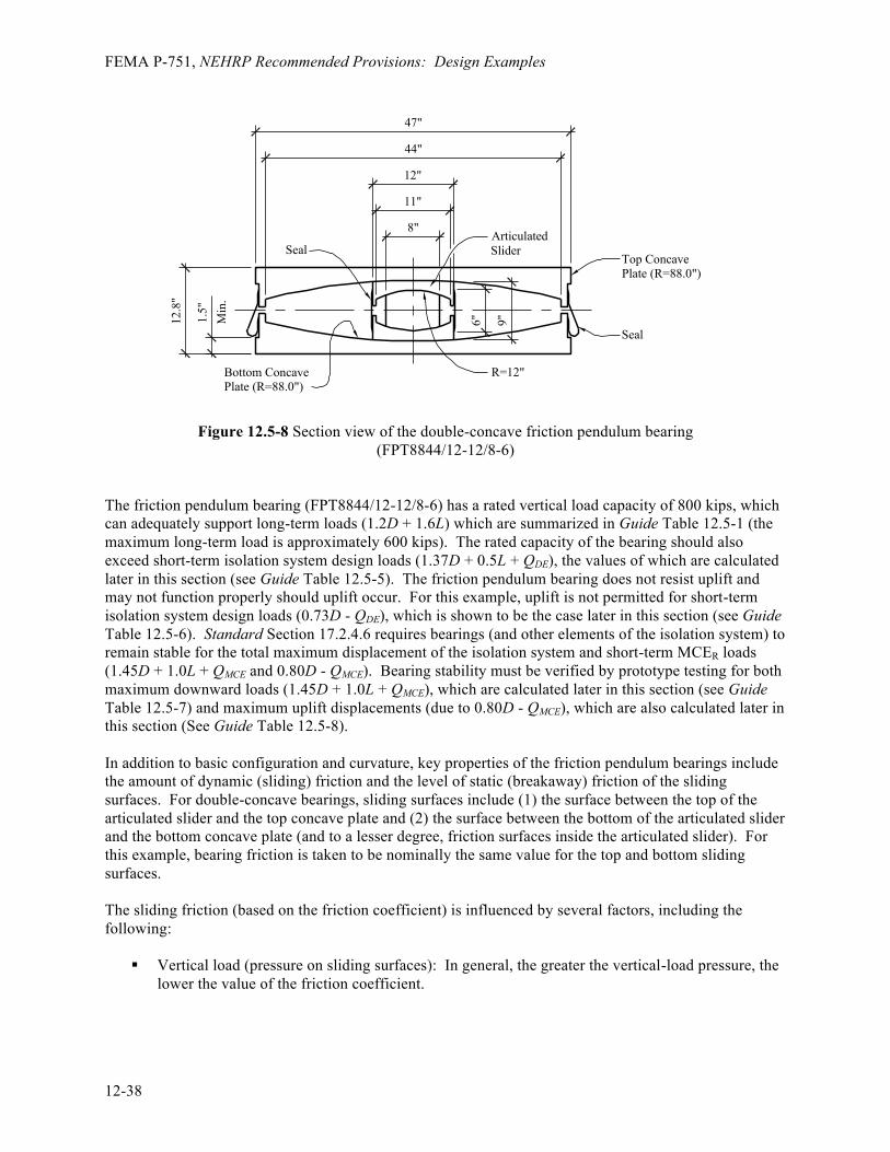
FEMA P-751, NEHRP Recommended Provisions: Design Examples
12-38
Figure 12.5-8 Section view of the double-concave friction pendulum bearing (FPT8844/12-12/8-6)
The friction pendulum bearing (FPT8844/12-12/8-6) has a rated vertical load capacity of 800 kips, which can adequately support long-term loads (1.2D + 1.6L) which are summarized in Guide Table 12.5-1 (the maximum long-term load is approximately 600 kips). The rated capacity of the bearing should also exceed short-term isolation system design loads (1.37D + 0.5L + QDE), the values of which are calculated later in this section (see Guide Table 12.5-5). The friction pendulum bearing does not resist uplift and may not function properly should uplift occur. For this example, uplift is not permitted for short-term isolation system design loads (0.73D - QDE), which is shown to be the case later in this section (see Guide Table 12.5-6). Standard Section 17.2.4.6 requires bearings (and other elements of the isolation system) to remain stable for the total maximum displacement of the isolation system and short-term MCER loads (1.45D + 1.0L + QMCE and 0.80D - QMCE). Bearing stability must be verified by prototype testing for both maximum downward loads (1.45D + 1.0L + QMCE), which are calculated later in this section (see Guide Table 12.5-7) and maximum uplift displacements (due to 0.80D - QMCE), which are also calculated later in this section (See Guide Table 12.5-8). In addition to basic configuration and curvature, key properties of the friction pendulum bearings include the amount of dynamic (sliding) friction and the level of static (breakaway) friction of the sliding surfaces. For double-concave bearings, sliding surfaces include (1) the surface between the top of the articulated slider and the top concave plate and (2) the surface between the bottom of the articulated slider and the bottom concave plate (and to a lesser degree, friction surfaces inside the articulated slider). For this example, bearing friction is taken to be nominally the same value for the top and bottom sliding surfaces. The sliding friction (based on the friction coefficient) is influenced by several factors, including the following:
§ Vertical load (pressure on sliding surfaces): In general, the greater the vertical-load pressure, the lower the value of the friction coefficient.
8"
11"
12"
44"
47"
1.5"
Min
.
12.8
"
Seal
Bottom ConcavePlate (R=88.0")
Seal
Top ConcavePlate (R=88.0")
ArticulatedSlider
9"6"
R=12"

Chapter 12: Seismically Isolated Structures
12-39
§ Rate of lateral load (bearing velocity): In general, the greater the velocity, the higher the value of the friction coefficient (although the friction coefficient tends to be fairly constant at moderate and high earthquake velocities).
§ Bearing temperature (surface temperature of sliding surfaces): In general, the hotter the bearing,
the lower the value of the friction coefficient. Bearings get hot due to repeated cycles of earthquake load. Bearing temperature is a function of the duration of earthquake shaking (the number of cycles of dynamic load) and the friction force on the sliding surface. The greater the number of cycles of dynamic load, the hotter the bearing. The greater the friction force (due to larger vertical load or friction coefficient), the hotter the bearing.
Other factors influencing friction and sliding bearing performance include manufacturing tolerances (not all bearings can be made exactly the same) and the effects of aging and possible contamination of sliding surfaces (which should be minimal for bearings with protective seals and not exposed to the environment). For the preliminary design of the isolation system (and subsequent analyses of the isolation system), nominal and bounding values of the siding friction coefficient are used to construct hysteresis loops that define effective stiffness, effective period and the effective damping of the isolations system (i.e., all 35 bearings acting together) as a function of isolation system displacement. For this example, the nominal value of the friction coefficient of top and bottom concave plates is µp,nom = 0.06, with a lower-bound value of µp,min = 0.04 and an upper-bound value of µp,max = 0.08 and the friction coefficient of the articulated slider (internal surfaces) is µs = 0.02. Static breakaway friction is assumed to be less than or equal to µp,max. A relatively large variation in the friction coefficient, a factor of 2, is used to bound all sources of friction coefficient variability, described above, including possible change in properties over the life of the bearing. As discussed later in Guide Section 12.5.6, isolation system properties based on assumed values must be verified by testing of isolator prototypes. The effective stiffness (normalized by building weight), keff,D/W, may be calculated approximately as a function of bearing displacement, D, in inches for the double-concave friction pendulum bearing, as follows:
where the term, µP, represents nominal, upper-bound or lower-bound value of the sliding friction coefficient, rp is the radius of the concave plates, hs is the height of the articulated slider, rs is the radius of the articulated slider and hc is the height of the core of the articulated slider. Similarly, the bi-linear concepts shown in Guide Figure 12.1-2 are used to calculate effective period, Teff,D and effective damping, βeff,D, as a function of bearing displacement, D, in inches for the double concave friction pendulum bearing, as follows:
,1/
2 2eff D PP s s c
k W Dr h r h
µ⎛ ⎞
= + ⎜ ⎟− + −⎝ ⎠
,,
0.32/eff D
eff D
DTk W
=
,,
,
/0.637
/y y eff D
eff Deff D
DF D k WDk W
β⎛ ⎞−
= ⎜ ⎟⎜ ⎟⎝ ⎠

FEMA P-751, NEHRP Recommended Provisions: Design Examples
12-40
where:
Figures 12.5-9, 12.5-10 and 12.5-11 are plots of effective stiffness, effective period and effective damping, respectively, based on the above formulas and the geometric and sliding friction properties of the double-concave friction pendulum bearing. These curves are useful design aids that are referred to in subsequent sections when determining amplitude-dependent properties of the isolation system.
Figure 12.5-9 Effective stiffness as a function of the displacement of the double-concave friction pendulum bearing (FPT8844/12-12/8-6)
( )2y P S SD dµ µ= −
12 2y P yP s s c
A Dr h r h
µ⎛ ⎞
= + ⎜ ⎟− + −⎝ ⎠
0.00
0.05
0.10
0.15
0.20
0.25
0 5 10 15 20 25 30
Nor
mal
ized
bea
ring
forc
e, F
/W
Bearing displacement (in.)

Chapter 12: Seismically Isolated Structures
12-41
Figure 12.5-10 Effective period as a function of the displacement of the double-concave friction pendulum bearing (FPT8844/12-12/8-6)
Figure 12.5-11 Effective damping as a function of the displacement of the double-concave friction pendulum bearing (FPT8844/12-12/8-6)
1.0
1.5
2.0
2.5
3.0
3.5
4.0
0 5 10 15 20 25 30
Effe
ctiv
e pe
riod
(s)
Bearing displacement (in.)
0%
5%
10%
15%
20%
25%
30%
35%
40%
0 5 10 15 20 25 30
Effe
ctiv
e da
mpi
ng
Bearing displacement (inches)

FEMA P-751, NEHRP Recommended Provisions: Design Examples
12-42
12.5.4.2 Calculation of design values. 12.5.4.2.1 Design displacements. Preliminary design begins with the engineer’s selection of the effective period (and effective damping) of the isolated structure and the calculation of the design displacements. This process is necessarily iterative, since the effective period (and effective damping) is amplitude dependent. In this example, the effective DE period of the EOC facility (i.e., effective period at design earthquake displacement) is estimated using lower-bound properties of Guide Figure 12.5-10 to be approximately TD = 3.5 seconds at a design displacement of DD = 16.0 inches, calculated using Standard Equation 17.5-1 as follows:
The 1.5 value of the damping coefficient, BD, is given in Standard Table 17.5-1 assuming 20 percent effective damping at 16.0 inches of isolation system displacement, which is consistent with lower-bound effective damping shown in Guide Figure 12.5-11. The same approach is used to estimate the MCER period, in this case TM = 3.9 seconds at a maximum displacement of approximately DM = 30 inches, calculated using Standard Equation 17.5-3 as follows:
The 1.3 value of the damping coefficient, BM, is given in Standard Table 17.5-1 assuming 13 percent effective damping at approximately 30 inches of isolation system displacement, which is consistent with lower-bound effective damping shown in Guide Figure 12.5-11. It may be noted from this figure that the effective damping of the isolation system and related benefits of reduced response decrease significantly with response amplitude at large displacements. The total displacement of specific isolator units (considering the effects of torsion) is calculated based on the plan dimensions of the building, the total torsion (due to actual, plus accidental eccentricity) and the distance from the center of resistance of the building to the isolator unit of interest. Using Standard Equations 17.5-5 and 17.5-6, the total design displacement, DTD and the total maximum displacement, DTM, of isolator units located on Column Lines 1 and 7 are calculated for the critical (transverse) direction of earthquake load to be approximately 20 percent greater than DD and DM, respectively. Standard Equations 17.5-5 and 17.5-6 assume that mass is distributed in plan in proportion to isolation system stiffness, offset by 5 percent, providing no special resistance to rotation of the building above the isolation system. These assumptions are reasonable, in general, but are not appropriate for isolation systems that have inherent resistance to torsion. For example, systems which have less load on bearings at the perimeter (as is the case of most buildings) and/or more stiffness at the perimeter (due to stiffer bearings) would not experience this amount of additional response due to torsion. For sliding systems, friction forces are roughly proportional to applied load and the center of resistance would tend to move with any change in the actual center of mass, such as that associated with accidental mass eccentricity. Accordingly, additional displacement due to accidental mass eccentricity is taken as 10 percent, the minimum value of additional displacement permitted by Standard Section 17.5.3.3. Applying a 10 percent increase to the design and maximum displacement values produces total design and maximum displacement (i.e., at building corners) values of DTD = 17.6 inches (1.1 × 16.0) and
( ) ( )12
0.7 3.59.8 16.0 in.
1.54D D
DD
S TgDBπ
⎛ ⎞= = =⎜ ⎟⎝ ⎠
( ) ( )12
1.05 3.99.8 30.9 in.
1.34M M
MM
S TgDBπ
⎛ ⎞= = =⎜ ⎟⎝ ⎠

Chapter 12: Seismically Isolated Structures
12-43
DTM = 34.0 inches (1.1 × 30.9), respectively, the latter of which is about the displacement capacity of the bearing. 12.5.4.2.2 Minimum and maximum effective stiffness. Standard Equation 17.5-2 expresses the effective period at the design displacement in terms of building weight (dead load) and the minimum effective stiffness of the isolation system, kDmin. Rearranging terms and solving for minimum effective stiffness results in the following:
Similarly, the minimum effective stiffness at the maximum displacement is calculated as follows:
Estimates of the maximum effective stiffness at the design displacement, DD = 16.0 inches and maximum displacement, DM = 30.9 inches, can be made using Guide Figure 12.5-9, which shows the upper-bound effective stiffness to be approximately 20 percent greater than the lower-bound effective stiffness at 16.0 inches and the upper-bound effective stiffness to be approximately 15 percent greater than lower-bound effective stiffness at 30.9 inches of displacement: As noted earlier, the range of effective stiffness illustrated in Guide Figure 12.5-9 represents the isolation system as a whole rather than the range of effective stiffness associated with individual bearings and is intended to address a number of factors that influence potential variation in bearing properties, including the effects of aging and contamination, etc. A report, Property Modification Factors for Seismic Isolation Bearings (Constantinou, 1999), provides guidance for establishing a range of effective stiffness (and effective damping) properties that captures various sources of the variation over the design life of the isolator units. The range of effective stiffness of the isolation system has a corresponding range of effective periods (with different levels of spectral demand). As discussed in Guide Section 12.3, the longest effective period (corresponding to the minimum effective stiffness) of the range is used to define isolation system design displacement and the shortest effective period (corresponding to the maximum effective stiffness) of the range is used to define the design forces on the superstructure. 12.5.4.2.3 Lateral design forces. The lateral force required for the design of the isolation system, foundation and other structural elements below the isolation system is given by Standard Equation 17.5-7: Vb = kDmax DD = 91.0(16.0) = 1,456 kips The lateral force required for checking stability and ultimate capacity of elements of the isolation system may be calculated as follows: VMCE = kMmax DM = 70.3(30.9) = 2,172 kips
2
min 2 24 1 9,100 75.8 kips/in.
9.8 3.5DD
Wkg Tπ⎛ ⎞ ⎛ ⎞
= = =⎜ ⎟ ⎜ ⎟⎝ ⎠⎝ ⎠
2
min 2 24 1 9,100 61.1 kips/in.
9.8 3.9MD
Wkg Tπ⎛ ⎞ ⎛ ⎞
= = =⎜ ⎟ ⎜ ⎟⎝ ⎠⎝ ⎠
max 1.2(75.8) 91.0 kips / in.Dk = =
max 1.15(61.1) 70.3 kips / in.Mk = =

FEMA P-751, NEHRP Recommended Provisions: Design Examples
12-44
The (unreduced) base shear of the design earthquake is approximately 16 percent of the weight of the EOC and the (unreduced) base shear of the MCE is approximately 24 percent of the weight. Subject to the limits of Standard Section 17.5.4.3, the design earthquake base shear, Vs, is reduced by the RI factor in accordance with Standard Equation 17.5-8:
This force is only approximately 8 percent of the dead load weight of the EOC, which is less than the limits of Item 3 of Section 17.5.4.3 that require a minimum base shear of at least 1.5 times the “break-away friction level of a sliding system.” In this example, breakaway friction is assumed to be less than or equal to the maximum value of sliding friction, µP,max = 0.08, such that the minimum design earthquake base shear, Vs, is calculated as follows: which is substantially less than the lateral force that would be required for the design of a conventional, fixed-base, EOC building of the same size and height, seismic force-resisting system and site seismic conditions. Story shear forces on the superstructure are distributed vertically over the height of the structure in accordance with Standard Equation 17.5-9, as shown in Table 12.5-4.
Table 12.5-4 Vertical Distribution of Reduced Design Earthquake Forces (Vs = 1,092 kips)
Floor level, x (Story)
Floor weight, wx
(kips)
Cumulative weight (kips)
Height above isolation
system, hx (ft)
Story force, Fx, (kips) (Standard
Eq. 17.5-9)
Cumulative story force
(kips)
Cum. force divided by cumulative
weight
PH Roof 794 54
(Penthouse) 794 196 196 25%
Roof 2,251 42
(Third) 3,045 432 628 21%
Third Floor 1,947 30
(Second) 4,992 267 895 18%
Second Floor 1,922 18
(First) 6,914 158 1,053 15%
First Floor 2,186 4
(Isolation) 9,100 40 1,092 12%
1.0 ft = 0.3048 m, 1.0 kip = 4.45 kN. Standard Equation 17.5-9 distributes lateral seismic design forces (Vs = 1.092 kips) over the height of the building’s superstructure in an inverted triangular pattern, effectively doubling shear force at the roof level, as indicated by values of cumulative story force divided by weight above shown in Table 12.5-4. Because the superstructure is much stiffer laterally than the isolation system, it tends to move as a rigid
max 91.0(16.0) 728 kips2.0
D Ds
I
k DVR
= = =
,max1.5 1.5(0.08)9,100 1,092 kipss PV Wµ= = =

Chapter 12: Seismically Isolated Structures
12-45
body, rather than in the first mode, with a pattern of lateral seismic forces that is typically more uniformly distributed over the height of the building. The use of a triangular load pattern for design is intended to account for higher-mode response that may be excited by superstructure flexibility and isolation system nonlinearity. Standard Equation 17.5-9 is also used to distribute forces over the height of the building for unreduced DE and MCER forces, as summarized in Table 12.5-5. Unreduced forces are required for design of isolator units.
Table 12.5-5 Vertical Distribution of Unreduced Design Earthquake and MCER Forces
Story
Design Earthquake Forces MCER Forces
Story force, Fx (kips)
(Standard Eq. 17.5-9)
Cumulative story force
(kips)
Cum. force divided by cumulative
weight
Story force, Fx (kips)
(Standard Eq. 17.5-9)
Cumulative story force
(kips)
Cum. force divided by cumulative
weight
Penthouse 261 261 33% 389 389 49%
Third 576 837 27% 859 1,248 41%
Second 356 1,192 24% 530 1,778 35%
First 211 1,403 20% 315 2,093 30%
Isolation 53 1,456 16% 79 2,172 24% 12.5.4.2.4 Design earthquake forces for isolator units. Tables 12.5-6 and 12.5-7 show the maximum and minimum downward forces for design of the isolator units. These forces result from the simultaneous application of gravity loads and unreduced design earthquake story forces, summarized in Table 12.5-5, to the ETABS model of the EOC. (See Guide Sec. 12.5.2.5 for the design load combinations.) As described in Guide Section 12.5.2.5, loads are applied separately in the two horizontal directions and results for both directions are reported in these tables (i.e., x direction / y direction). All values in Table 12.5-7 are positive, indicating that uplift does not occur at any bearing location for unreduced DE loads.
Table 12.5-6 Maximum Downward Force (kips) for Isolator Design (1.37D + 0.5L + QDE)*
Maximum downward force (kips)
Line 1 2 3 4
A 225 / 225 383 / 498 334 / 356 336 / 359
B 480 / 389 590 / 668 674 / 700 633 / 812
C 349 / 328 641 / 709 632 / 631 586 / 570 1.0 kip = 4.45 kN * Forces at Column Lines 5, 6 and 7 (not shown) are similar to those at Column Lines 3, 2 and 1, respectively; loads at
Column Lines D and E (not shown) are similar to those at Column Lines B and A, respectively.
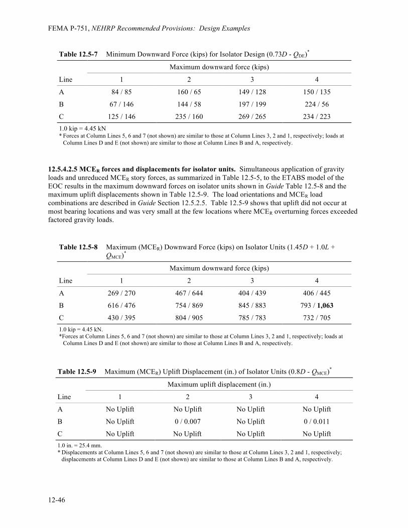
FEMA P-751, NEHRP Recommended Provisions: Design Examples
12-46
Table 12.5-7 Minimum Downward Force (kips) for Isolator Design (0.73D - QDE)*
Maximum downward force (kips)
Line 1 2 3 4
A 84 / 85 160 / 65 149 / 128 150 / 135
B 67 / 146 144 / 58 197 / 199 224 / 56
C 125 / 146 235 / 160 269 / 265 234 / 223 1.0 kip = 4.45 kN * Forces at Column Lines 5, 6 and 7 (not shown) are similar to those at Column Lines 3, 2 and 1, respectively; loads at
Column Lines D and E (not shown) are similar to those at Column Lines B and A, respectively.
12.5.4.2.5 MCER forces and displacements for isolator units. Simultaneous application of gravity loads and unreduced MCER story forces, as summarized in Table 12.5-5, to the ETABS model of the EOC results in the maximum downward forces on isolator units shown in Guide Table 12.5-8 and the maximum uplift displacements shown in Table 12.5-9. The load orientations and MCER load combinations are described in Guide Section 12.5.2.5. Table 12.5-9 shows that uplift did not occur at most bearing locations and was very small at the few locations where MCER overturning forces exceeded factored gravity loads.
Table 12.5-8 Maximum (MCER) Downward Force (kips) on Isolator Units (1.45D + 1.0L + QMCE)*
Maximum downward force (kips)
Line 1 2 3 4
A 269 / 270 467 / 644 404 / 439 406 / 445
B 616 / 476 754 / 869 845 / 883 793 / 1,063
C 430 / 395 804 / 905 785 / 783 732 / 705 1.0 kip = 4.45 kN. *Forces at Column Lines 5, 6 and 7 (not shown) are similar to those at Column Lines 3, 2 and 1, respectively; loads at
Column Lines D and E (not shown) are similar to those at Column Lines B and A, respectively.
Table 12.5-9 Maximum (MCER) Uplift Displacement (in.) of Isolator Units (0.8D - QMCE)*
Maximum uplift displacement (in.)
Line 1 2 3 4
A No Uplift No Uplift No Uplift No Uplift
B No Uplift 0 / 0.007 No Uplift 0 / 0.011
C No Uplift No Uplift No Uplift No Uplift 1.0 in. = 25.4 mm. * Displacements at Column Lines 5, 6 and 7 (not shown) are similar to those at Column Lines 3, 2 and 1, respectively;
displacements at Column Lines D and E (not shown) are similar to those at Column Lines B and A, respectively.

Chapter 12: Seismically Isolated Structures
12-47
12.5.4.2.6 Limits on dynamic analysis. The displacements and forces determined by the ELF procedure provide a basis for expeditious assessment of size and capacity of isolator units and the required strength of the superstructure. The results of the ELF procedure also establish limits on design parameters when dynamic analysis is used as the basis for design. Specifically, the total design displacement, DTD and the total maximum displacement of the isolation system, DTM, determined by dynamic analysis cannot be less than 90 percent and 80 percent, respectively, of the corresponding ELF procedure values: DTD, dynamic ≥ 0.9DTD, ELF = 0.9(17.6) = 15.8 in. DTM, dynamic ≥ 0.8DTM, ELF = 0.8(34.0) = 27.2 in. Similarly, the lateral force, Vb, required for design of the isolation system, foundation and all structural elements below the isolation system and the lateral force, Vs, required for design of the superstructure determined by dynamic analysis are limited to 90 percent and 80 percent, respectively, of the ELF procedure values: Vb, dynamic ≥ 0.9Vb, ELF = 0.9(1,456) = 1,310 kips (= 0.144W) Vs, dynamic ≥ 0.8Vs, ELF = 0.8(1,092) = 874 kips (= 0.096W) As an exception to the above, lateral forces less than 80 percent of the ELF results are permitted for design of superstructures of regular configuration, if justified by response history analysis (which is seldom, if ever, the case). However, Vs,dynamic is also subject to the limits of Section 17.5.4.3 for response history analysis (and also, by inference, for response spectrum analysis) which govern the value of Vs,ELF in this example and thus govern the minimum value of design base shear (regardless of the analysis method used for design): Vs, dynamic ≥ Vs, ELF = 1.0(1,092) = 1,092 kips (= 0.12W) 12.5.4.3 Preliminary design of the superstructure. The lateral forces, developed in the previous section, in combination with gravity loads, provide a basis for preliminary design of the superstructure, using methods similar to those used for a conventional building. In this example, selection of member sizes was made based on the results of ETABS model calculations. Detailed descriptions of the design calculations are omitted, since the focus of this section is on design aspects unique to isolated structures (i.e., the design of the isolation system, which is described in the next section). Figures 12.5-12 and 12.5-13 are elevation views at Column Lines 2 and B, respectively. Figure 12.5-14 is a plan view of the building that shows the framing at the first floor level.

FEMA P-751, NEHRP Recommended Provisions: Design Examples
12-48
Figure 12.5-12 Elevation of framing on Column Lines 2 ,4 and 6
Third Floor
Base
First Floor
Second Floor
Roof
Penthouse RoofW18x76W18x76
W18x76W18x76 W18x76W18x76
W18x76 W18x76 W18x76 W18x76
W18x76W18x76W18x76W18x76
W24x146W24x146W24x146W24x146HSS10x10x5/8
HSS10x10x5/8
HSS10x10x5/8
HSS10x10x5/8
W14
x132
W14
x132
W14
x68
W14
x132
W14
x132
W14
x132
W14
x68
W14
x68
W14
x68
W14
x68
W14
x68
W14
x132
W14
x132
W14
x132
W14
x68
W14
x68
W14
x68
W14
x68
HSS10x10x5/8
HSS10x10x5/8
HSS10x10x5/8
HSS10x10x5/8
W14
x132
W14
x132
W14
x132
W14
x132
W14
x132
Third Floor
Base
First Floor
Second Floor
Roof
Penthouse RoofW18x76W18x76
W18x76W18x76 W18x76W18x76
W18x76 W18x76 W18x76 W18x76
W18x76W18x76W18x76W18x76
W24x146W24x146W24x146W24x146
HSS12x12x1/2
W14
x132
W14
x132
W14
x132
W14
x132
W14
x132
W14
x132
W14
x68
W14
x68
W14
x68
W14
x68
W14
x68
W14
x132
W14
x132
W14
x68
W14
x68
W14
x68
W14
x68
W14
x68
HSS12x12x1/2
HSS12x12x1/2
HSS12x12x1/2
W14
x132
W14
x132
W14
x132
W14
x132
W14
x132
a) Lines 2 and 6
b) Line 4
HSS12x12x1/2
HSS12x12x1/2
E D C B A
E D C B A

Chapter 12: Seismically Isolated Structures
12-49
Figure 12.5-13 Elevation of framing on Column Lines B and D
Figure 12.5-14 First floor framing plan
Penthouse Roof
Roof
Third Floor
Second Floor
First Floor
Base
W18x76 W18x76 W18x76 W18x76
W18x76W18x76W18x76W18x76W18x76
W18x76W18x76W18x76W18x76W18x76
W18x76W18x76W18x76W18x76W18x76W18x76
W24x146W24x146W24x146W24x146W24x146W24x146W14
x68
W14
x68
W14
x68
W14
x132
W14
x68
W14
x68
W14
x132
W14
x132
W14
x132
W14
x132
W14
x132
W14
x132
W14
x132
W14
x132
W14
x68
W14
x132
W14
x68
W14
x68
W14
x68
W14
x68
W14
x68
W14
x68
W14
x68
W14
x68
W14
x132
W14
x68
HSS10x10x5/8 HSS10x10x5/8
HSS10x10x5/8
HSS10x10x5/8
HSS10x10x5/8
HSS10x10x5/8
HSS10x10x5/8
HSS10x10x5/8
HSS10x10x5/8
HSS10x10x5/8
HSS10x10x5/8
W18x76
W18x76
1 2 3 4 5 6 7W
14x1
32
W14
x132
W14
x132
W14
x132
W14
x132
W14
x132
W14
x132
W24 x146
W24
x14
6
W24 x146 W24 x146 W24 x146 W24 x146 W24 x146
W24 x146W24 x146W24 x146W24 x146W24 x146W24 x146
W24 x146W24 x146W24 x146W24 x146W24 x146W24 x146
W24 x146W24 x146W24 x146W24 x146W24 x146W24 x146
W24 x146W24 x146W24 x146W24 x146W24 x146W24 x146
W24
x14
6W
24 x
146
W24
x14
6
W16
x26
W24
x14
6W
24 x
146
W24
x14
6W
24 x
146
W24
x14
6W
24 x
146
W24
x14
6W
24 x
146
W24
x14
6W
24 x
146
W24
x14
6W
24 x
146
W24
x14
6W
24 x
146
W24
x14
6W
24 x
146
W24
x14
6W
24 x
146
W24
x14
6W
24 x
146
W24
x14
6W
24 x
146
W24
x14
6W
24 x
146
1 2 3 4 5 6 7
A
B
C
D
E
W16
x26
W16
x26
W16
x26
W16
x26
W16
x26
W16
x26
W16
x26
W16
x26
W16
x26
W16
x26
W16
x26
W16
x26
W16
x26
W16
x26
W16
x26
W16
x26
W16
x26
W16
x26
W16
x26
W16
x26
W16
x26
W16
x26
W16
x26
W16
x26
W16
x26
W16
x26
W16
x26
W16
x26
W16
x26
W16
x26
W16
x26
W16
x26
W16
x26
W16
x26
W16
x26
W16
x26
W16
x26
W16
x26
W16
x26
W16
x26
W16
x26
W16
x26
W16
x26
W16
x26
W16
x26
W16
x26
W16
x26
FEMA P-751, NEHRP Recommended Provisions: Design Examples
12-50
As shown in the elevations (Figures 12.5-12 and 12.5-13), relatively large (HSS 10×10×5/8) tubes are conservatively used throughout the structure for diagonal bracing. A quick check of these braces indicates that stresses will be at or below yield for earthquake loads. For example, the four braces at the third story, on Lines 2, 4 and 6 (critical floor and direction of bracing) resist a reduced design earthquake force of approximately 175 kips (628 kips / 4 braces × cos[25°]), on average. The corresponding average brace stress is only approximately 8 ksi (for reduced design earthquake forces) and only approximately 11 ksi and 16 ksi for unreduced DE and MCER earthquake forces, respectively, indicating that the structure is expected to remain elastic even for MCER demand. As shown in Figure 12.5-14, the first-floor framing has relatively heavy, W24×146 girders along lines of bracing (Lines B, D, 2, 4 and 6). These girders resist P-delta moments as well as other forces. A quick check of these girders indicates that only limited yielding is likely, even for the MCER loads (and approximately 3 feet of MCER displacement). Girders on Line 2 that frame into the column at Line B (critical columns and direction of framing) resist a P-delta moment due to the MCER force of approximately 800 kip-ft (1,063 kips / 2 girders × 3 feet / 2). Additional moment in these girders due to MCER shear force in isolators is approximately 500 kip-ft (1,063 kips × 0.24 × 4 feet / 2 girders). Thus, total moment is approximately 1,300 kips due to gravity and MCER loads (and 3 feet of MCER displacement), which is conservatively less than the plastic capacity of these girders (i.e., φbMp = 1,570 kip-ft). 12.5.4.4 Isolator connection detail. The isolation system has a similar detail at each column for the example EOC, as shown in Figure 12.5-15. The column has a large, stiffened base plate that bears directly on the top of the isolator unit. The column base plate is circular, with a diameter comparable to that of the top plate of the isolator unit. Heavy, first-floor girders frame into and are moment connected to the columns (moment connections are required at this floor only). The columns and base plates are strengthened by plates that run in both horizontal directions, from the bottom flange of the girder to the base. Girders are stiffened above the seat plates and at temporary jacking locations. The top plate of the isolator unit is bolted to the column base plate and the bottom plate of the isolator unit is bolted to the foundation. The foundation (and grout) directly below the isolator must have sufficient strength to support concentrated bearing loads from the concave plate and articulated slider above (for all possible lateral displacements of the isolator). Similarly, the column base plate and structure just above the isolator must have sufficient strength to transfer concentrated bearing loads to the concave plate and articulated slider below. The foundation connection accommodates the removal and replacement of isolator units, as required by Standard Section 17.2.4.8. Anchor bolts pass through holes in this plate and connect to threaded couplers that are attached to deeply embedded rods. Figure 12.5-15 illustrates connection details typical of isolated structures; other details could be developed that work just as well and certainly details would be different for structures that have a different configuration or material.

Chapter 12: Seismically Isolated Structures
12-51
Figure 12.5-15 Typical detail of the isolation system at columns (for clarity, some elements are not shown)
With the exception of the portion of the column above the first-floor slab, each element shown in Figure 12.5-11 is an integral part of the isolation system (or foundation) and is designed for the gravity and unreduced design earthquake loads. In particular, the first-floor girder, the connection of the girder to the column and the connection of the column to the base plate are designed for gravity loads and forces caused by horizontal shear and P-delta effects due to the unreduced design earthquake loads (as shown earlier in Guide Figure 12.4-1).
12.5.5 Design Verification Using Nonlinear Response History Analysis
The Standard requires dynamic analysis for design of isolated buildings like the example EOC that are located at sites with 1-second spectral acceleration, S1, greater than or equal to 0.6g (see Guide Table 12.2-1). The Standard also requires that the dynamic analysis requirement be satisfied using response history analysis (RHA) for isolated buildings like the example EOC that have an isolation systems that does not fully comply with the criteria of Item 7 of Standard Section 17.4.1. In practice it is common to use the RHA procedure to verify the design of structures with sliding or high-damping isolation systems. This example uses RHA to determine final design displacements of the isolation system and to confirm that ELF-based forces used for preliminary design of the superstructure and isolation system are valid. While results of RHA could be used to refine the preliminary design of the superstructure (e.g., reduce size of lateral bracing, etc.), this example uses RHA primarily for “design verification” of key global
W12x120
W24x146is
olat
orun
it
(milled) heavy plate
grout
nut
bolt
bolt or threaded rodinto coupler

FEMA P-751, NEHRP Recommended Provisions: Design Examples
12-52
response parameters (i.e., confirmation of ELF-based story shear force). If the RHA procedure were used as the primary basis for superstructure design, then response results would be required for design of individual elements, rather than for checking a limited number of global response parameters. 12.5.5.1 Ground motion records. The RHA procedure evaluates DE and MCER response of the example EOC using the set of seven ground motion records previously described in Guide Section 12.5.4.4. Seven records are used for RHA so that the average value of the response parameter of interest can be used for design (or design verification). Each record has two horizontal components, one of which is identified as the “larger” component in terms of spectral acceleration at the effective period of the isolation system (i.e., 3.9 seconds). The ground motion records are grouped (oriented) in terms of the larger component (Step 2) and are applied to the analytical model (Step 4) in accordance with procedure recommended in Guide Sec. 12.4.4. Guide Table 12.5-2 summarizes key source and site properties used as the basis for record selection and Guide Table 12.5-3 summarizes factors used to scale each record to match design earthquake and MCER response spectra, respectively. Guide Figure 12.5-7 compares the average spectra of the seven scaled records (for the SRSS combination of components and the larger component, respectively) with the MCER response spectrum demonstrating compliance with scaling requirements of Standard Section 17.3.2 and the recommendations of Guide Section 12.4.4 (Step 3). 12.5.5.2 ETABS models. The ETABS computer program is used for RHA of analytical models of the isolated structure, as previously discussed in Guide Section 12.5.3. Two basic ETABS models are developed for RHA analysis, both having the same superstructure but representing lower-bound and upper-bound stiffness properties of isolators (FP bearings), respectively. Elements of the superstructure and isolation system (other than the isolators) are modeled as linear elastic elements based on member sizes developed by preliminary design (Guide Section 12.5.4.3). Elements are not expected to yield significantly, even for MCER response and the assumption of linear elastic behavior is quite reasonable. For RHA, ETABS internally calculates modal damping based on the hysteretic properties of the nonlinear elements (isolators) and an additional amount of user-specified modal damping. For the EOC example, additional damping is limited to 2 percent of critical for all modes, since the steel superstructure remains essentially linear elastic. Two types of isolator nonlinearity are modeled explicitly. First, gap elements, just above each isolator, model potential uplift of the isolation system. The gap elements transmit downward (compressive) forces but release and permit upward displacement of the structure, if upward (tension) forces occur. The purpose of the gap elements is to check for possible uplift due to overturning loads exceeding factored gravity loads and to calculate the maximum amount of vertical displacement, should uplift occur. The second type of isolator nonlinearity is that associated with horizontal force-deflection properties of isolators. For this example, nonlinear force-deflection properties of the isolator units are modeled using the ETABS nonlinear “Isolator2” element. This element was originally developed for FP bearing with a single concave plate and requires the user to input the initial stiffness (effective stiffness before the articulated slider displaces on the concave plate), the friction coefficient properties and the radius of the concave plate. For the double concave FP bearing of this example, an “effective” radius, reff, is used to account for simultaneous sliding of the articulated slider on the two concave plates. The effective radius, reff, of the two dishes is 185 inches, based on the radius of each concave plate (rp = 88 inches), the height of the articulated slider (hs = 9 inches), the radius of the articulated slider (rs = 12 inches) and the height of the internal core (hc = 6 inches):
Chapter 12: Seismically Isolated Structures
12-53
reff = 2rp - hs + 2rs - hc = 2 × 88 in. - 9 in. + 2 × 12 in. - 6 in. = 185 inches The Isolator2 element simulates bilinear, hysteretic behavior commonly used to model the nonlinear properties of friction-pendulum bearings, although the double-concave configuration generally requires more sophisticated representation of bearing properties. For example, very complex models of this bearing have been developed and implemented in 3D-BASIS (Constantinou, et al.) and SAP2000 (CSI). Use of these more sophisticated models would be required for double-concave friction pendulum bearings configured to have different friction coefficients for the surfaces of top and bottom concave plates, respectively, or for projects which explicitly model the stiffening effects of articulated slider engagement with the boundary of concave plates. Such modeling is not required for the EOC example and the bilinear curve of the Isolator2 element (available in ETABS) is used for design verification. The Isolator2 element requires the user to input three sliding friction parameters: (1) the “fast” value of the sliding coefficient of friction, (2) the “slow” value of the sliding coefficient of friction and (3)a “rate” parameter that essentially governs transition between slow and fast properties (e.g., when the bearing reaches peak displacement and reverses direction of travel). For the Isolator2 element, “fast” represents velocities in excess of approximately 1 to 2 inches per second. Typically, during strong ground motions, such as those of this example, sliding velocities are well in excess of 2 inches per second and isolation system response is dominated by “fast” sliding friction properties. Lower-bound and upper-bound values of sliding friction coefficient are used to represent lower-bound and upper-bound values FP bearing of “stiffness,” as previously discussed in Guide Section 12.5.4.1. Lower-bound and upper-bound values of sliding friction coefficient, 4 percent and 8 percent respectively, are used to model “fast” sliding friction properties of the FP bearings. One-half of these values, 2 percent and 4 percent respectively, are used to model “slow” sliding friction properties. These values are consistent with observed behavior (“slow” properties are approximately one-half of “fast” properties) and have little influence on peak dynamic response. Figure 12.5-16 illustrates hysteresis loops based on upper-bound and lower-bound stiffness properties of FP bearings, normalized by vertical load (P). The slope of these loops is proportional to the inverse of the effective radius (185 inches) and the thickness (vertical height) of these loops is twice the value of the sliding friction coefficient. The upper-bound loop, plotted to DD = 16 inches, is based on 8 percent sliding friction and the lower-bound loop, plotted to DM = 30.9 inches, is based on 4 percent sliding friction. The hysteresis loops shown in Figure 12.5-16 could be modeled using appropriate values of bilinear element. While the bearings of this example all have identical properties, stiffness varies as a function of vertical load (since friction force is a function of vertical load). Thus, values of the initial stiffness (a required parameter of the Isolator2 element of ETABS) are a function of vertical load. While technically different for each bearing, the same value of initial stiffness is assumed for bearings that have similar amounts of vertical load. Table 12.5-10 provides values of initial FP bearing stiffness for three bearing load groups (regions): Region A: bearings at interior column locations with heavier loads (15 locations), Region B: bearings at perimeter column locations, except corners (16 locations) and Region C: bearings at corner columns with lighter loads (4 locations). Similarly, Table 12.5-11 shows values of effective isolator stiffness, corresponding to 16 inches of peak design earthquake and 30.9 inches of peak MCER response, respectively. Values of effective stiffness shown in Table 12.5-11 are not required for response history analysis but would be required (along with corresponding values of the damping coefficient) for response spectrum analysis using ETABS.
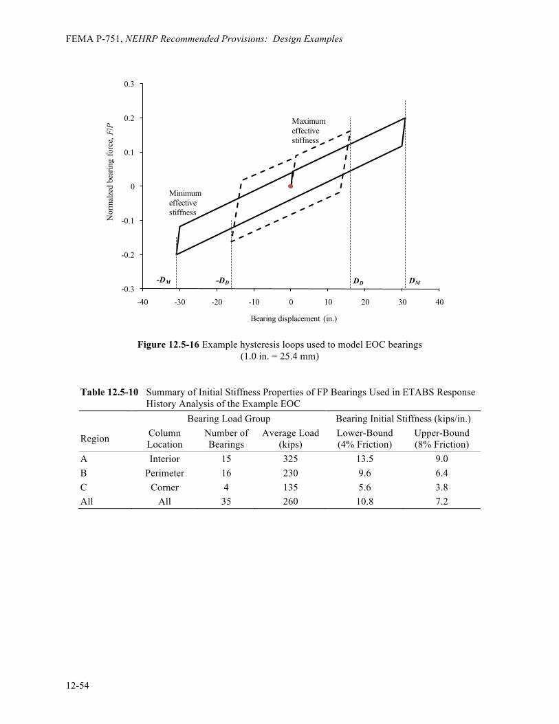
FEMA P-751, NEHRP Recommended Provisions: Design Examples
12-54
Figure 12.5-16 Example hysteresis loops used to model EOC bearings (1.0 in. = 25.4 mm)
Table 12.5-10 Summary of Initial Stiffness Properties of FP Bearings Used in ETABS Response History Analysis of the Example EOC
Bearing Load Group Bearing Initial Stiffness (kips/in.)
Region Column Location
Number of Bearings
Average Load (kips)
Lower-Bound (4% Friction)
Upper-Bound (8% Friction)
A Interior 15 325 13.5 9.0 B Perimeter 16 230 9.6 6.4 C Corner 4 135 5.6 3.8 All All 35 260 10.8 7.2
DM-DM DD-DD-0.3
-0.2
-0.1
0
0.1
0.2
0.3
-40 -30 -20 -10 0 10 20 30 40
Nor
mal
zed
bear
ing
forc
e, F
/P
Bearing displacement (in.)
Maximumeffective stiffness
Minimumeffective stiffness

Chapter 12: Seismically Isolated Structures
12-55
Table 12.5-11 Summary of Effective Stiffness Properties of FP Bearings of the Example EOC Building (Appropriate for Response Spectrum Analysis)
Bearing Load Group
Bearing Effective Stiffness (kips/in.) Design Earthquake Response
(at DD = 16.0 in.) MCER Response (at DM = 30.9 in.)
Region Lower-Bound (4% Friction)
Upper-Bound (8% Friction)
Lower-Bound (4% Friction)
Upper-Bound (8% Friction)
A 2.57 3.38 2.18 2.60 B 1.82 2.39 1.54 1.84 C 1.07 1.40 0.90 1.08 All 2.06 2.71 1.74 2.08
For isolators with known properties, parameters defining bilinear stiffness may be based on test data provided by the manufacturer. For example, Figure 12.5-17 compares hysteresis loops based on upper-bound and lower-bound stiffness properties (normalized by weight) with actual hysteresis loops of cyclic load tests of a prototype of the double-concave friction pendulum bearing. In this case, design loops are constructed for the same peak displacement (approximately 30 inches) as that of the prototype test. Test results indicate an average effective stiffness (normalized by vertical load) of keff/P = 0.0074 kip/in./kip at 30 inches of peak displacement that is well bounded by maximum and minimum values of effective stiffness kMmin = 0.0067 kip/in./kip (1.74 kips/in. / 260 kips) to kMmax = 0.0080 kip/in./kip (2.08 kips/in. / 260 kips), respectively. Test results also indicate an average effective damping of approximately 18 percent for the three cycles of prototype testing, which supports the use of an effective damping value, βM = 15 percent, for calculating MCER response (ELF procedure).
Figure 12.5-17 Comparison of modeled and tested hysteresis loops for EOC bearings (1.0 in. = 25.4 mm, 1.0 kip/in. = 0.175 kN/mm)
12.5.5.3 Analysis process. The two primary ETABS models, incorporating lower-bound (4 percent sliding friction) and upper-bound (8 percent sliding friction) properties are analyzed for the set of seven ground motion records applied to the models in each of four orientations of the larger component of
-0.3
-0.2
-0.1
0
0.1
0.2
0.3
-40 -30 -20 -10 0 10 20 30 40Horizontal displacement (in.)
V/W

FEMA P-751, NEHRP Recommended Provisions: Design Examples
12-56
records with respect to the primary horizontal axes of the model: (1) positive X-axis direction, (2) negative X-axis direction, (3) positive Y-axis direction and (4) negative Y-axis direction, respectively. The average value of the parameter of interest is calculated for each of four record set orientations and the more critical value of positive and negative orientations of the record set is used for design verification in the (x or y) direction of interest (e.g., story shear in the x direction). The more critical value of each of the four record set orientations is used for design verification when the response parameter of interest is not direction dependent (e.g., peak isolation system displacement). This process is repeated for ground motion records scaled to DE and MCER spectral accelerations. Although a large number of data are generated by these analyses, only limited number of response parameters is required for design verification. Response parameters of interest include the following:
§ Design Earthquake:
1. Peak isolation system displacement
2. Peak story shear forces (envelope over building height)
§ Maximum Considered Earthquake:
1. Peak isolation system displacement
2. Peak downward load on any isolator unit (1.45D + 1.0L + QMCE)
3. Peak uplift displacement of any isolator unit (0.8D - QMCE). 12.5.5.4 Summary of results of response history analyses. RHA results are generally consistent with and support design values based on ELF formulas. The ETABS model with lower-bound stiffness properties (4 percent sliding friction) governs peak isolation system displacements. The lower-bound stiffness model also governs peak uplift displacement of isolators. The ETABS model with upper-bound stiffness properties (8 percent sliding friction) governs peak story shear forces and peak downward loads on isolators, although the value of the response parameters typically are similar for the two ETABS models. Specific results are summarized and compared to ELF values in the following sections. 12.5.5.4.1 Peak isolation system displacement. Table 12.5-12 summarizes peak isolation system displacements calculated by RHA for DE and MCER ground motions (average displacement of seven records). RHA results show the larger value of peak displacements in the X-axis and Y-axis directions and the peak displacement in the X-Y plane. Total displacement (at corners due to rotation) is based on the minimum 10 percent increase due to accidental mass eccentricity for both ELF and RHA results. Results of the evaluation of uplift are also included in Table 12.5-12.

Chapter 12: Seismically Isolated Structures
12-57
Table 12.5-12 Summary of Peak DE and MCER Displacements of the Isolation System Calculated Using RHA (Average Displacement of Seven Records) and Comparison with DE and MCER Displacements Calculated Using ELF Formulas
Response Parameter Method of Analysis
ELF Formulas RHA - Average of Seven Records
Maximum (X, Y) X-Y Plane Design Earthquake - Isolation System Displacement (inches)
Design (Center) 16.0 15.0 15.9 Total (Corner) 17.6 16.5 17.5 Uplift NA No uplift (all records)
MCER - Isolation System Displacement (inches) MCER (Center) 30.9 28.2 29.6 Total (Corner) 34.0 31.1 32.5 Uplift NA Less than 0.01 in. (2/7 records) The average value of peak DE displacement in the X-Y plane is 15.9 inches, as compared to 16.0 inches calculated using ELF formulas. The average value of peak MCER displacement is 29.6 inches, as compared to 30.8 inches calculated using ELF formulas. The total DE displacement is found to be 17.5 inches and the total MCER displacement is found to be 32.5 inches (including a 10 percent increase in displacement to account for the effects of accidental mass eccentricity not explicitly modeled in the RHA analysis). Peak isolation system displacements calculated using RHA are slightly less than the corresponding values determined by ELF formulas, but within the RHA limits (minimum) based on ELF formulas (see Guide Section 12.5.4.2.6). The total MCER displacement of 32.6 inches is just less than the 33-inch displacement capacity of the FP bearing (displacement at which the articulated slider would engage the restraining edge of concave plates). Uplift did not occur at bearing locations for the DE ground motions. A very small amount of uplift occurred during two of the seven MCER ground motion records, which is less than but consistent with the amount of uplift previously determined by nonlinear static (pushover) analysis (see Guide Table 12.5-8). The Standard does not require the response of individual records to be used for design, or design verification, where seven or more records are used for RHA. Nonetheless, it is prudent to consider the implications of the results of individual record analyses and it is helpful to use ELF formulas to evaluate RHA results (serving as a sanity check on results). Table 12.5-12 summarizes peak displacements calculated by RHA for individual records scaled to DE and MCER ground motions. The results in this table are based on an application of records with the larger components aligned with the X-axis direction of the model. RHA results show values of peak displacement in the X-axis and Y-axis directions and in the X-Y plane. A couple of observations may be made. First, the peak displacement in the direction of the larger component is almost the same, on average, as the peak response in the X-Y plane. The second observation that may be made is that the displacement response varies greatly between records and that this variation is correlated directly with the variation of spectral response at long periods. For example, peak design earthquake displacement of Record Number NF-25 (the Yarmica record from the 1999 Kocaeli earthquake) is 30.7 inches in the X-Y plane (30.5 inches in the X-axis direction), which is less than the unrestrained displacement capacity of the FP bearing, but approximately twice the average
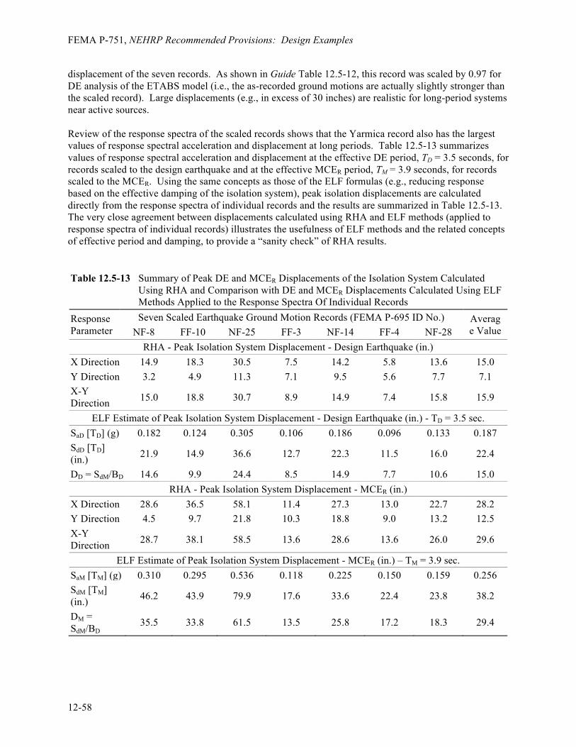
FEMA P-751, NEHRP Recommended Provisions: Design Examples
12-58
displacement of the seven records. As shown in Guide Table 12.5-12, this record was scaled by 0.97 for DE analysis of the ETABS model (i.e., the as-recorded ground motions are actually slightly stronger than the scaled record). Large displacements (e.g., in excess of 30 inches) are realistic for long-period systems near active sources. Review of the response spectra of the scaled records shows that the Yarmica record also has the largest values of response spectral acceleration and displacement at long periods. Table 12.5-13 summarizes values of response spectral acceleration and displacement at the effective DE period, TD = 3.5 seconds, for records scaled to the design earthquake and at the effective MCER period, TM = 3.9 seconds, for records scaled to the MCER. Using the same concepts as those of the ELF formulas (e.g., reducing response based on the effective damping of the isolation system), peak isolation displacements are calculated directly from the response spectra of individual records and the results are summarized in Table 12.5-13. The very close agreement between displacements calculated using RHA and ELF methods (applied to response spectra of individual records) illustrates the usefulness of ELF methods and the related concepts of effective period and damping, to provide a “sanity check” of RHA results. Table 12.5-13 Summary of Peak DE and MCER Displacements of the Isolation System Calculated
Using RHA and Comparison with DE and MCER Displacements Calculated Using ELF Methods Applied to the Response Spectra Of Individual Records
Response Parameter
Seven Scaled Earthquake Ground Motion Records (FEMA P-695 ID No.) Average Value NF-8 FF-10 NF-25 FF-3 NF-14 FF-4 NF-28
RHA - Peak Isolation System Displacement - Design Earthquake (in.) X Direction 14.9 18.3 30.5 7.5 14.2 5.8 13.6 15.0 Y Direction 3.2 4.9 11.3 7.1 9.5 5.6 7.7 7.1 X-Y Direction 15.0 18.8 30.7 8.9 14.9 7.4 15.8 15.9
ELF Estimate of Peak Isolation System Displacement - Design Earthquake (in.) - TD = 3.5 sec. SaD [TD] (g) 0.182 0.124 0.305 0.106 0.186 0.096 0.133 0.187 SdD [TD] (in.) 21.9 14.9 36.6 12.7 22.3 11.5 16.0 22.4
DD = SdM/BD 14.6 9.9 24.4 8.5 14.9 7.7 10.6 15.0 RHA - Peak Isolation System Displacement - MCER (in.)
X Direction 28.6 36.5 58.1 11.4 27.3 13.0 22.7 28.2 Y Direction 4.5 9.7 21.8 10.3 18.8 9.0 13.2 12.5 X-Y Direction 28.7 38.1 58.5 13.6 28.6 13.6 26.0 29.6
ELF Estimate of Peak Isolation System Displacement - MCER (in.) – TM = 3.9 sec. SaM [TM] (g) 0.310 0.295 0.536 0.118 0.225 0.150 0.159 0.256 SdM [TM] (in.) 46.2 43.9 79.9 17.6 33.6 22.4 23.8 38.2
DM = SdM/BD 35.5 33.8 61.5 13.5 25.8 17.2 18.3 29.4

Chapter 12: Seismically Isolated Structures
12-59
Table 12.5-13 shows that the peak MCER displacement for two scaled records (Yarmica and Arcelik) exceeds the 33-inch displacement capacity of the FP bearing—that is, the articulated slider will engage and be restrained by the concave plates. Such engagement would reduce displacement of the isolation system but also increase story shear force and overturning loads and increase the possibility of damage to the isolation system and the superstructure. It should be expected that displacements calculated for one or two records of a set of seven records scaled to match an MCER response spectrum for a site close to an active fault will exceed the average displacement of the set, even by as much as by a factor of two. The Standard requires design for the average and therefore tacitly accepts that displacements calculated for some records will be larger than the average displacement required for design of the isolation system. It would be prudent, however, for designers to consider the consequences of the very unlikely event that the MCER displacement is exceeded in an actual earthquake. In the case of the example EOC, displacements larger than MCER displacement would be expected to cause damage to the bearings, but not catastrophic failure of the isolation system or superstructure. The concave plates (and surrounding moat) would limit displacement of the isolation system (i.e., the isolation system would not displace laterally to failure). As the bearings (and surrounding moat) limit displacement, forces would increase significantly in the seismic force-resisting system of the structure above, comparable to peak response of a conventional (fixed-base) building. Yielding and inelastic response would likely occur, but the Standard requirement that special framing (e.g., SCBF) be used for the superstructure provides the requisite ductility to inelastically resist the response due to impact restraint of isolators (and the surrounding moat). 12.5.5.4.2 Peak story shear force. Table 12.5-14 summarizes story shear force results in the X-axis and Y-axis directions and compares these values with story shear forces calculated by ELF formulas for unreduced design earthquake loads. Figure 12.5-17 shows story shears calculated by ELF formulas and by RHA methods. Table 12.5-14 and Figure 12.5-18 show the inherent (and intentional) conservatism of the ELF formulas, which assume an inverted triangular pattern of lateral loads to account for potential higher-mode effects. The example EOC has minimal contribution from higher modes, as reflected in the lower values of story shear at upper floor and roof elevations. For the example EOC, design story shear forces are based on the limits of Standard Section 17.5.4.3 (Vs = 1.5 × 0.08W = 0.12W, where 0.08W represents the “breakaway” friction level of a sliding system), which apply to all methods of analysis, including RHA.
Table 12.5-14 Summary of Peak Design Story Shear Forces and Comparison with Design Earthquake Story Shear Values Calculated Using ELF Methods
Response Parameter Method of Analysis
ELF Formulas Peak RHA Result
X-axis Direction Y-axis Direction Design Earthquake - Story Shear (kips)
Penthouse 261 150 147 Third Story 837 546 531 Second Story 1,192 874 855 First Story 1,403 1,183 1,173 Vb (Isolators) 1,456 1,440 1,449

FEMA P-751, NEHRP Recommended Provisions: Design Examples
12-60
Figure 12.5-18 Comparison of story shear force based on RSA and ELF procedures
12.5.5.4.3 Peak downward loads on isolators. Table 12.5-15 summarizes maximum downward forces on isolator units determined from the MCER response history analyses. This table reports the two values for each isolator location representing both the X-axis and Y-axis orientations of the larger component of shaking of the ground motion record.
Table 12.5-15 Maximum Downward Force (kips) on Isolator Units (1.45D + 1.0L + QMCE)*
Maximum downward force (kips)
Line 1 2 3 4
A 247 / 245 512 / 532 376 / 383 378 / 385
B 534 / 512 639 / 637 753 / 764 796 / 825
C 380 / 371 718 / 726 707 / 707 620 / 620 1.0 kip = 4.45 kN. * Forces at Column Lines 5, 6 and 7 (not shown) are similar to those at Column Lines 3, 2 and 1, respectively; loads at
Column Lines D and E (not shown) are similar to those at Column Lines B and A, respectively.
0
10
20
30
40
50
0 200 400 600 800 1,000 1,200 1,400 1,600
Eele
vatio
n (f
eet)
Story shear force (kips)
Average results of RHA
ELF

Chapter 12: Seismically Isolated Structures
12-61
Table 12.5-15 indicates a maximum downward force of 825 kips (at Column B4), which is somewhat less than the maximum value of downward force predicted using the ELF (pushover) methods (1,063 kips in Guide Table 12.5-7). The difference between RHA and ELF results reflects differences in overturning loads and patterns of story shear forces shown in the previous section. For this example, RHA results are used to verify ELF (pushover) values, but they could play a more meaningful role in reducing overturning loads for projects with a more challenging configuration of the superstructure.
12.5.6 Design and Testing Criteria for Isolator Units
Detailed design of the isolator units typically is the responsibility of the manufacturer subject to the design and testing (performance) criteria included in the construction documents (drawings and/or specifications). Performance criteria typically include a basic description and size(s) of isolator units; design life, durability, environmental loads and fire-resistance criteria; quality assurance and quality control requirements (including QC testing of production units); design criteria (loads, displacements, effective stiffness and damping); and prototype testing requirements. This section summarizes the design criteria and prototype testing requirements for the isolator units (FP bearings) of the example EOC. 12.5.6.1 Bearing design loads.
§ Maximum Long-Term Load (from Table 12.5-1, Col. C3): 1.2D + 1.6L = 600 kips
§ Maximum Short-Term Load (from Tables 12.5-8/12.5-15, Col. B4): 1.45D + 1.0L + |E| = 1,000 kips
§ Minimum Short-Term Load (from Table 12.5-9, Col. B4): 0.8D - |E| = 0 kips (less than 0.1 inch
of uplift)
§ For Cyclic-Load Testing (Standard Sec. 17.8.2.2): Typical Load (Table 12.5-1, average all bearings): 1.0D + 0.5L = 290 kips Upper-Bound Load (Table 12.5-6, average all bearings): 1.37D + 0.5L + QDE = 500 kips Lower-Bound Load (Table 12.5-7, average all bearings): 0.73D - QDE = 150 kips Item 2 of Standard Section 17.8.2.2 requires that cyclic tests at different displacement amplitudes be performed for typical vertical load (1.0D + 0.5L) and for upper-bound and lower-bound values of vertical load (for load-bearing isolators) where upper-bound and lower-bound loads are based on the load combinations of Standard Section 17.2.4.6 (vertical load stability). The load combinations of Standard Section 17.2.4 define “worst case” MCER loading conditions for checking isolator stability. In the opinion of the author, these load combinations are, in general, too extreme for cyclic load testing to verify isolator response properties (at lower levels of response). For the EOC example, upper-bound and lower-bound values of vertical load are based (roughly) on average bearing load at peak design earthquake response, as defined by the loads in Tables 12.5-6 and 12.5-7, respectively. The range of vertical load, from 150 kips to 500 kips, addresses the intent of the cyclic testing requirements (i.e., to measure possible variation in effective stiffness and damping properties). 12.5.6.2 Bearing design displacements (Table 12.5-12).
§ Design earthquake displacement: DD = 16 in.

FEMA P-751, NEHRP Recommended Provisions: Design Examples
12-62
§ Total design earthquake displacement: DTD = 17.5 in.
§ Maximum considered earthquake displacement: DM = 30 in.
§ Total maximum considered earthquake displacement: DTM = 32.5 in.
12.5.6.3 Bearing effective stiffness and damping criteria.
§ Minimum effective stiffness normalized by load (typical vertical load): Design earthquake displacement : kDmin ≥ 0.0079 kips/in./kip Maximum considered earthquake displacement: kMmin ≥ 0.0067 kips/in./kip
§ Maximum effective stiffness normalized by weight (typical vertical load): Design earthquake displacement: kDmax ≤ 0.0104 kips/in./kip Maximum considered earthquake displacement: kMmax ≤ 0.0080 kips/in./kip The kDmin, kDmax, kMmin and kMmax criteria are properties of the isolation system as a whole (calculated from the properties of individual isolator units using Standard Equations 17.8-3 through 17.8-6). The above limits on effective stiffness of the isolation system include changes in isolator properties over the life of the structure (due to contamination, aging, etc.), as well as other effects that may not be addressed by prototype testing (e.g., changes in properties under repeated cycles of dynamic load). Ideally, prototype bearings would have properties near the center of the specified range of effective stiffness. Effective damping (typical vertical load):
§ Design earthquake displacement: βD ≥ 20 percent
§ Maximum considered earthquake displacement: βM ≥ 13 percent 12.5.6.4 Prototype bearing testing criteria. Standard Section 17.8 prescribes a series of prototype tests to establish and validate design properties used for design of the isolation system and defines “generic” acceptance criteria (Sec. 17.8.2) with respect to force-deflection properties of test specimens. Table 12.5-16 summarizes the sequence and cycles of prototype testing found in Standard Section 17.8.2, applicable to the FP bearing of the example EOC.
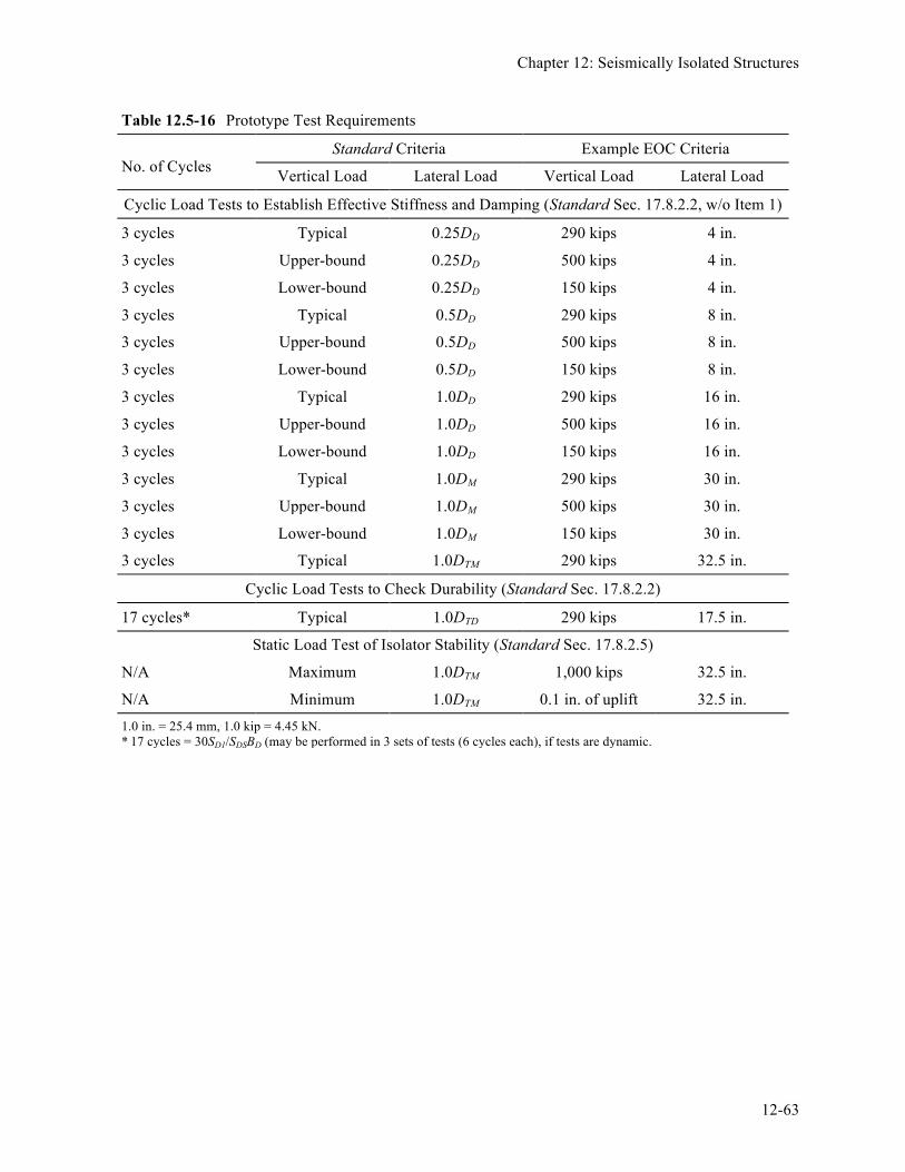
Chapter 12: Seismically Isolated Structures
12-63
Table 12.5-16 Prototype Test Requirements
No. of Cycles Standard Criteria Example EOC Criteria
Vertical Load Lateral Load Vertical Load Lateral Load
Cyclic Load Tests to Establish Effective Stiffness and Damping (Standard Sec. 17.8.2.2, w/o Item 1)
3 cycles Typical 0.25DD 290 kips 4 in.
3 cycles Upper-bound 0.25DD 500 kips 4 in.
3 cycles Lower-bound 0.25DD 150 kips 4 in.
3 cycles Typical 0.5DD 290 kips 8 in.
3 cycles Upper-bound 0.5DD 500 kips 8 in.
3 cycles Lower-bound 0.5DD 150 kips 8 in.
3 cycles Typical 1.0DD 290 kips 16 in.
3 cycles Upper-bound 1.0DD 500 kips 16 in.
3 cycles Lower-bound 1.0DD 150 kips 16 in.
3 cycles Typical 1.0DM 290 kips 30 in.
3 cycles Upper-bound 1.0DM 500 kips 30 in.
3 cycles Lower-bound 1.0DM 150 kips 30 in.
3 cycles Typical 1.0DTM 290 kips 32.5 in.
Cyclic Load Tests to Check Durability (Standard Sec. 17.8.2.2)
17 cycles* Typical 1.0DTD 290 kips 17.5 in.
Static Load Test of Isolator Stability (Standard Sec. 17.8.2.5)
N/A Maximum 1.0DTM 1,000 kips 32.5 in.
N/A Minimum 1.0DTM 0.1 in. of uplift 32.5 in. 1.0 in. = 25.4 mm, 1.0 kip = 4.45 kN. * 17 cycles = 30SD1/SDSBD (may be performed in 3 sets of tests (6 cycles each), if tests are dynamic.


![The Behavior of Multi-Story Buildings Seismically Isolated ...file.scirp.org/pdf/OJER_2014121817203398.pdf · Isolated System Hybrid Isolation ... [11]. The importance of ... -This](https://img.dokumen.tips/doc/110x75/5b348ac87f8b9a8b4b8c2651/the-behavior-of-multi-story-buildings-seismically-isolated-filescirporgpdfojer.jpg)