Embed Size (px)
Citation preview
Petroleum Geoscience
doi: 10.1144/petgeo2011-0432013, v.19; p21-38.Petroleum Geoscience
M.A. Martin, M. Wakefield, M.K. MacPhail, T. Pearce and H. E. Edwards play: Walloon Subgroup of the Surat Basin, eastern AustraliaSedimentology and stratigraphy of an intra-cratonic basin coal seam gas
serviceEmail alerting to receive free e-mail alerts when new articles cite this article hereclick
requestPermission to seek permission to re-use all or part of this article hereclick
Subscribe to subscribe to Petroleum Geoscience or the Lyell Collection hereclick
Notes
© The Geological Society of London 2013
at BG International Ltd on February 3, 2013http://pg.lyellcollection.org/Downloaded from
Petroleum Geoscience, Vol. 19, 2013, pp. 21 –38 DOI: 10.1144/petgeo2011-043
1354-0793/13/$15.00 © 2013 EAGE/Geological Society of London
An appreciation of the Surat Basin’s geology will be key to the successful undertaking of the first ever coal seam gas to liquefied natural gas programme and critical to the evaluation of the gas-in-place. To better understand the depositional sys-tem and the correlation and connectivity of the coals a pilot, in-house, integrated sedimentology, biostratigraphy and chem-ostratigraphy study was carried out. Three broad facies associ-ations are recognized and the preliminary findings of the bio- and chemostratigraphical studies test the regional extent of the finer stratigraphical subdivisions.
The facies are based solely on detailed sedimentological analysis of three wells spread across the basin. The associated stratigraphical study focused on three closely spaced wells from the basin centre. These penetrate the whole of the Walloon Subgroup. One well is common to both studies. Of prime inter-est are the interrelationships and connectivity of the facies in the context of building large-scale geo-models for volumetric and reserve calculations and well planning.
IntroductIon
Coal-bearing strata are complex heterolithic sedimentary suc-cessions. The geometry of coal and associated clastic facies can exhibit a high degree of complexity that can be difficult to interpret, in the absence of outcrop, even in closely spaced wells (Leblang et al. 1981). To accumulate thick coal succes-sions requires a balance between peat production and accom-modation space development allowing the preservation of terrigenous organic matter (Diessel 1992; Bohacs & Suter 1997; Wadsworth et al. 2002; Jerrett et al. 2011a, b). By studying the relationships of the resultant coals and their associated facies, fluctuations in accommodation space can be recognized. These intuitively might relay information about the scale of the coal bodies and their possible correlatability.
The majority of models presented for coal succession are derived from coastal settings or sections with marine influence (Diessel 1992; Flores et al. 1999; Diessel et al. 2000; Jerrett et al. 2011a, b) The Walloon Subgroup (WSG) in the Surat Basin is entirely non-marine (Exon & Burger 1981) and, as such, many depositional models are inappropriate.
Data, in this study, were analysed from wells in the Walloons CSG ‘fairway’. This is defined in the Surat Basin, by reservoir depth, thickness, stratigraphical limit, gas content, gas satura-tions and coal permeability (Fig. 1).
Over 600 wells have been drilled through the WSG within the Queensland Gas Company (QGC) tenements (licensed acre-age). Of these, more than 80 have been extensively cored, pro-viding a rich dataset with the potential to study this complex system without the need to resort to analogues. As a precursor to such work a stratigraphic framework and broad understanding of the depositional elements is required. A series of pilot studies were carried out to assess regional variation in sedimentary facies and the correlation of these units. In the pilot sedimentol-ogy study, core was examined from three wells (1, 4 and 5, see Fig. 1), selected so as to provide as broad a geographical cover-age as possible, to highlight any potential regional variations in facies. There was no intention to correlate these widely (c. 80 km) spaced wells. The WSG is 300–450 m thick in the study wells and fully cored. Concurrently, a pilot stratigraphical study selected wells (wells 2, 3 and 4) focused on demonstrating proof-of-concept correlation in this previously poorly palynolog-ically studied basin, these wells were approximately 8 km apart. One well was common to both the sedimentology and strati-graphical studies (well 4).
The ultimate aim of the pilots was to test the ability to pro-vide a robust stratigraphic framework from which regional varia-tions in reservoir (coal) properties could be observed, and a framework for static reservoir models. The facies information
Sedimentology and stratigraphy of an intra-cratonic basin coal seam gas play: Walloon Subgroup of the Surat Basin, eastern Australia
M.A. Martin1*, M. Wakefield1, M.K. MacPhail2, t. Pearce3 and H. E. Edwards3
1BG Group, 100 Thames Valley Park, Reading RG61PT, UK2Department of Archaeology and Natural History, Australian National University, Canberra,
ACT 0200, Australia3Chemostrat Ltd., Unit 1, Ravenscroft Court, Buttington Cross Enterprise Park, Welshpool,
Powys SY21 8SL, UK*Corresponding author (e-mail: [email protected])
ABStrAct: Large gas reserves are trapped in the coals of the Middle Juras-sic (Callovian) Walloon Subgroup (lower part of the Injure Creek Group) in the Surat Basin, eastern Australia. The series is divided into the Juandah Coal Measures (upper), Tangalooma Sandstone and Taroom Coal Measures (lower). The upper and lower units are locally further subdivided. These economically important coals were deposited in an alluvial plain setting within an interior basin, which has no recorded contemporaneous marine influence. The coals are typically bituminous, perhydrous and low rank with a high volatile content. Despite individual ply (bench) thicknesses typically less than a metre, series of plies or seams of coals up to 10 m thick have historically been tentatively cor-related across the entire play area (over 150 km).
2011-043research-articleArticle19X10.1144/petgeo2011-043M. A. MartinWalloon Subgroup sedimentology and stratigraphy2013
at BG International Ltd on February 3, 2013http://pg.lyellcollection.org/Downloaded from
M. A. Martin et al.22
too would provide insights into the sedimentology and would provide a basis for understanding the reservoir distribution in the subsurface which should be reflected in the reservoir models.
Whilst tempting to use analogues for the reservoir modelling, with such a rich dataset (over 600 wells, some only tens of metres apart) the reservoir modelling parameters, reservoir thickness, connectivity and correlatability lie within the well data. Analogues have been used to help conceptualize the potential complexity of the coal connectivity, graphically as per US Geological Survey publications in the Paleocene Fort Union coals (e.g. Flores et al. 1999); to provide useful visual references for the spatial relation-ship of the depositional and geomorphic elements and facies asso-ciations for the non-coal facies (e.g. Ob River and Okavango River); whilst previous well correlations in the WSG, elsewhere in the Surat Basin (e.g. Jones & Patrick 1981; Leblang et al. 1981) help define coal correlatability. Unfortunately the WSG crop out poorly and so provide little additional data, but open-cast pits where the WSG are mined have provided other workers with useful facies information (e.g. Fielding 1993).
GEoloGIcAl SEttInG
The Surat Basin is a large (approximately 300 000 km2) Jurassic intra-cratonic basin in eastern Australia (Fig. 1) that overlies the Permo-Triassic Bowen Basin (Fig. 2). The basins have slightly offset depositional and structural axes (Fielding et al. 1990), and the Surat Basin is significantly less structur-ally complex (see Fig. 2). For an introduction to the geological setting, structural history, exploration history and broad stratig-raphy, readers are referred to Scott et al. (2007). The Surat Basin is part of the larger ‘Great Artesian Basin’ complex which continues westward into the Eromanga Basin and east-ward into the Clarence–Moreton Basin. The basin underwent continued thermal subsidence and was infilled by fluvial, lacustrine and mire (coal) sediments, with no recorded marine influence (Exon 1976).
Six major sedimentary cycles are recognized in the Jurassic–Cretaceous succession of the Surat Basin, each commencing with high-energy braided channel deposits and culminating in low-energy meandering rivers, lakes and mires (Jones & Patrick 1981; Turner et al. 2009). The fluvial–lacustrine deposition of
the WSG represents the end of one of these cycles, which started with the Hutton Sandstone (Fig. 3). This cycle is the K sequence of Hoffmann et al. (2009). Jones & Patrick (1981) proposed a higher order of cyclicity in the WSG; the first being from the Hutton to the Taroom Coal Measures and the second from the Tangalooma to the Juandahs, each representing a period of sta-bility and upwardly decreased fluvial activity.
The WSG pass laterally to the west into more coal-poor and lacustrine-dominated sediments of the Birkhead Fm. (Swarbrick et al. 1973). The WSG was deposited during the Middle Jurassic (Callovian), a ‘greenhouse’ period (see Fig. 3), when the Australian continent lay in high latitudes (Bradshaw & Yeung 1990). The first marine sediments in the Surat Basin occur in the Early Cretaceous (Exon & Burger 1981).
Throughout the Jurassic–Cretaceous, volcanism was perva-sive. It was thought to be centred away to the east of the basin (Exon 1976; Fielding 1993) but also possibly intra-basinal (Yago & Fielding 1996). Ash-fall tuffs occur commonly throughout the WSG.
Studies employed the lithostratigraphical nomenclature of the WSG, as defined by Scott et al. (2004, 2007; Fig. 3).
SEdIMEntoloGIcAl AnAlySIS
Some 1500 m of core from three wells (see Fig. 1) were logged in detail (1: 50 or 1: 200 scales). Prior to logging, the core was slabbed and photographed and the desorption samples (separated at well site) were re-united with the main core. A number of sandstone samples were taken for petrographical analysis and all proved to be immature lith-arenites. The coals were typically ‘dull’, bituminous, low rank, with high volatile content. A small number of sandstone ‘plugs’ were taken for core analysis, which demonstrated a porosity range of 9–10% and an average kh of 0.01 mD. A significant amount of coal-related desorption data, maceral analysis and permeability data (<10 to >500 mD) were generated. Full wireline log suites were available for the wells.
Sedimentary facies of the Walloon Subgroup
From the detailed core description, 21 individual facies grouped into three facies associations (primary channel, overbank and
�������
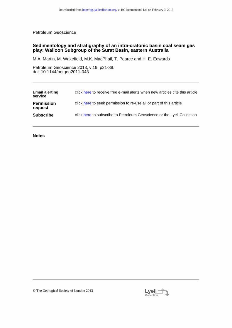
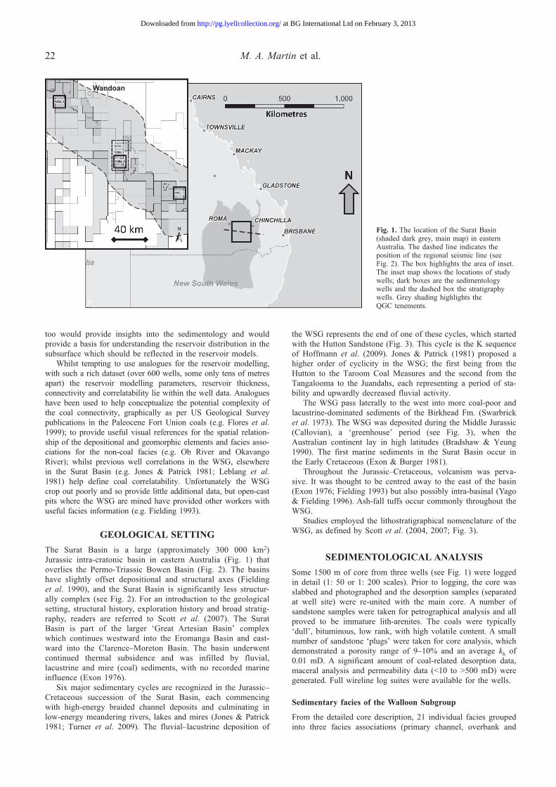
Fig. 1. The location of the Surat Basin (shaded dark grey, main map) in eastern Australia. The dashed line indicates the position of the regional seismic line (see Fig. 2). The box highlights the area of inset. The inset map shows the locations of study wells; dark boxes are the sedimentology wells and the dashed box the stratigraphy wells. Grey shading highlights the QGC tenements.
at BG International Ltd on February 3, 2013http://pg.lyellcollection.org/Downloaded from
Walloon Subgroup sedimentology and stratigraphy 23
����������
����������
�����������
��������
� ����������
�
���
���
���
���
���
���
���
���������
������
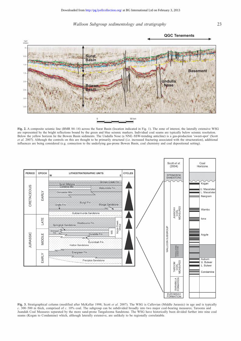
Fig. 2. A composite seismic line (BMR 84–14) across the Surat Basin (location indicated in Fig. 1). The zone of interest, the laterally extensive WSG are represented by the bright reflections bound by the green and blue seismic markers. Individual coal seams are typically below seismic resolution. Below the yellow horizon lie the Bowen Basin sediments. The Undulla Nose (a NNE–SSW-trending anticline) is a gas-production ‘sweet-spot’ (Scott et al. 2007). Although the controls on this are thought to be primarily structural (i.e. increased fracturing associated with the structuration), additional influences are being considered (e.g. connection to the underlying gas-prone Bowen Basin, coal chemistry and coal depositional setting).
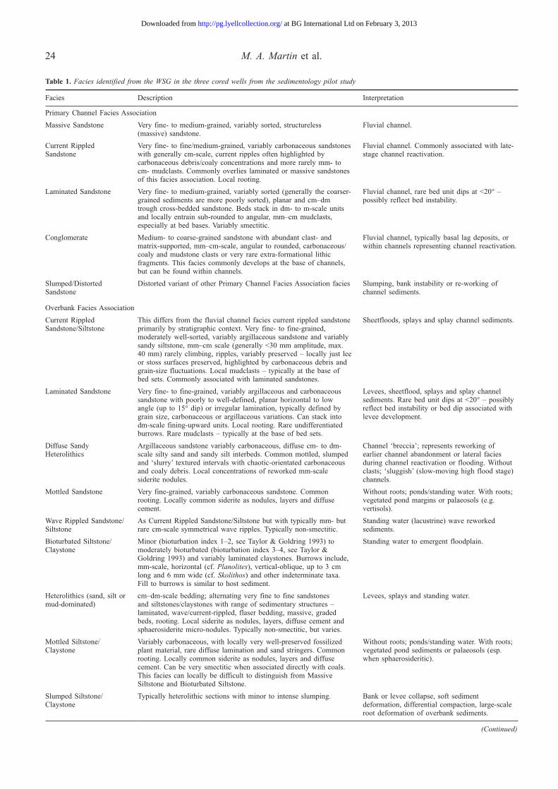
Fig. 3. Stratigraphical column (modified after McKellar 1998; Scott et al. 2007). The WSG is Callovian (Middle Jurassic) in age and is typically c. 300–500 m thick, comprised of c. 10% coal. The subgroup can be subdivided broadly into two major coal-bearing measures; Tarooms and Juandah Coal Measures separated by the more sand-prone Tangalooma Sandstone. The WSG have historically been divided further into nine coal seams (Kogan to Condamine) which, although laterally extensive, are unlikely to be regionally correlatable.
at BG International Ltd on February 3, 2013http://pg.lyellcollection.org/Downloaded from
M. A. Martin et al.24
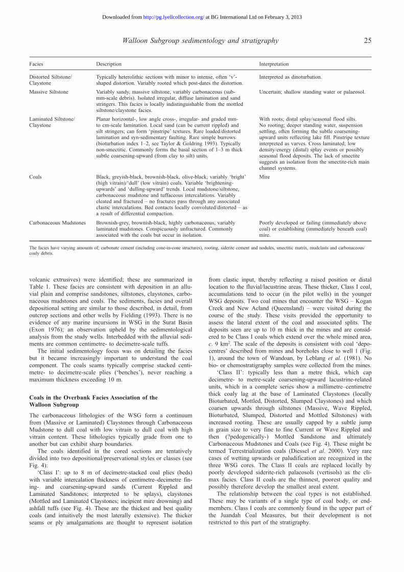
table 1. Facies identified from the WSG in the three cored wells from the sedimentology pilot study
Facies Description Interpretation
Primary Channel Facies Association
Massive Sandstone Very fine- to medium-grained, variably sorted, structureless (massive) sandstone.
Fluvial channel.
Current Rippled Sandstone
Very fine- to fine/medium-grained, variably carbonaceous sandstones with generally cm-scale, current ripples often highlighted by carbonaceous debris/coaly concentrations and more rarely mm- to cm- mudclasts. Commonly overlies laminated or massive sandstones of this facies association. Local rooting.
Fluvial channel. Commonly associated with late-stage channel reactivation.
Laminated Sandstone Very fine- to medium-grained, variably sorted (generally the coarser-grained sediments are more poorly sorted), planar and cm–dm trough cross-bedded sandstone. Beds stack in dm- to m-scale units and locally entrain sub-rounded to angular, mm–cm mudclasts, especially at bed bases. Variably smectitic.
Fluvial channel, rare bed unit dips at <20° – possibly reflect bed instability.
Conglomerate Medium- to coarse-grained sandstone with abundant clast- and matrix-supported, mm–cm-scale, angular to rounded, carbonaceous/coaly and mudstone clasts or very rare extra-formational lithic fragments. This facies commonly develops at the base of channels, but can be found within channels.
Fluvial channel, typically basal lag deposits, or within channels representing channel reactivation.
Slumped/Distorted Sandstone
Distorted variant of other Primary Channel Facies Association facies Slumping, bank instability or re-working of channel sediments.
Overbank Facies Association
Current Rippled Sandstone/Siltstone
This differs from the fluvial channel facies current rippled sandstone primarily by stratigraphic context. Very fine- to fine-grained, moderately well-sorted, variably argillaceous sandstone and variably sandy siltstone, mm–cm scale (generally <30 mm amplitude, max. 40 mm) rarely climbing, ripples, variably preserved – locally just lee or stoss surfaces preserved, highlighted by carbonaceous debris and grain-size fluctuations. Local mudclasts – typically at the base of bed sets. Commonly associated with laminated sandstones.
Sheetfloods, splays and splay channel sediments.
Laminated Sandstone Very fine- to fine-grained, variably argillaceous and carbonaceous sandstone with poorly to well-defined, planar horizontal to low angle (up to 15° dip) or irregular lamination, typically defined by grain size, carbonaceous or argillaceous variations. Can stack into dm-scale fining-upward units. Local rooting. Rare undifferentiated burrows. Rare mudclasts – typically at the base of bed sets.
Levees, sheetflood, splays and splay channel sediments. Rare bed unit dips at <20° – possibly reflect bed instability or bed dip associated with levee development.
Diffuse Sandy Heterolithics
Argillaceous sandstone variably carbonaceous, diffuse cm- to dm-scale silty sand and sandy silt interbeds. Common mottled, slumped and ‘slurry’ textured intervals with chaotic-orientated carbonaceous and coaly debris. Local concentrations of reworked mm-scale siderite nodules.
Channel ‘breccia’; represents reworking of earlier channel abandonment or lateral facies during channel reactivation or flooding. Without clasts; ‘sluggish’ (slow-moving high flood stage) channels.
Mottled Sandstone Very fine-grained, variably carbonaceous sandstone. Common rooting. Locally common siderite as nodules, layers and diffuse cement.
Without roots; ponds/standing water. With roots; vegetated pond margins or palaeosols (e.g. vertisols).
Wave Rippled Sandstone/Siltstone
As Current Rippled Sandstone/Siltstone but with typically mm- but rare cm-scale symmetrical wave ripples. Typically non-smectitic.
Standing water (lacustrine) wave reworked sediments.
Bioturbated Siltstone/Claystone
Minor (bioturbation index 1–2, see Taylor & Goldring 1993) to moderately bioturbated (bioturbation index 3–4, see Taylor & Goldring 1993) and variably laminated claystones. Burrows include, mm-scale, horizontal (cf. Planolites), vertical-oblique, up to 3 cm long and 6 mm wide (cf. Skolithos) and other indeterminate taxa. Fill to burrows is similar to host sediment.
Standing water to emergent floodplain.
Heterolithics (sand, silt or mud-dominated)
cm–dm-scale bedding; alternating very fine to fine sandstones and siltstones/claystones with range of sedimentary structures – laminated, wave/current-rippled, flaser bedding, massive, graded beds, rooting. Local siderite as nodules, layers, diffuse cement and sphaerosiderite micro-nodules. Typically non-smectitic, but varies.
Levees, splays and standing water.
Mottled Siltstone/Claystone
Variably carbonaceous, with locally very well-preserved fossilized plant material, rare diffuse lamination and sand stringers. Common rooting. Locally common siderite as nodules, layers and diffuse cement. Can be very smectitic when associated directly with coals. This facies can locally be difficult to distinguish from Massive Siltstone and Bioturbated Siltstone.
Without roots; ponds/standing water. With roots; vegetated pond sediments or palaeosols (esp. when sphaerosideritic).
Slumped Siltstone/Claystone
Typically heterolithic sections with minor to intense slumping. Bank or levee collapse, soft sediment deformation, differential compaction, large-scale root deformation of overbank sediments.
(Continued)
at BG International Ltd on February 3, 2013http://pg.lyellcollection.org/Downloaded from
Walloon Subgroup sedimentology and stratigraphy 25
volcanic extrusives) were identified; these are summarized in Table 1. These facies are consistent with deposition in an allu-vial plain and comprise sandstones, siltstones, claystones, carbo-naceous mudstones and coals. The sediments, facies and overall depositional setting are similar to those described, in detail, from outcrop sections and other wells by Fielding (1993). There is no evidence of any marine incursions in WSG in the Surat Basin (Exon 1976); an observation upheld by the sedimentological analysis from the study wells. Interbedded with the alluvial sedi-ments are common centimetre- to decimetre-scale tuffs.
The initial sedimentology focus was on detailing the facies but it became increasingly important to understand the coal component. The coals seams typically comprise stacked centi-metre- to decimetre-scale plies (‘benches’), never reaching a maximum thickness exceeding 10 m.
coals in the overbank Facies Association of the Walloon Subgroup
The carbonaceous lithologies of the WSG form a continuum from (Massive or Laminated) Claystones through Carbonaceous Mudstone to dull coal with low vitrain to dull coal with high vitrain content. These lithologies typically grade from one to another but can exhibit sharp boundaries.
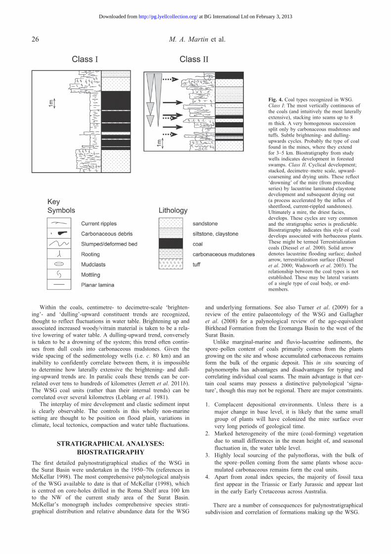
The coals identified in the cored sections are tentatively divided into two depositional/preservational styles or classes (see Fig. 4):
‘Class I’: up to 8 m of decimetre-stacked coal plies (beds) with variable intercalation thickness of centimetre–decimetre fin-ing- and coarsening-upward sands (Current Rippled and Laminated Sandstones; interpreted to be splays), claystones (Mottled and Laminated Claystones; incipient mire drowning) and ashfall tuffs (see Fig. 4). These are the thickest and best quality coals (and intuitively the most laterally extensive). The thicker seams or ply amalgamations are thought to represent isolation
from clastic input, thereby reflecting a raised position or distal location to the fluvial/lacustrine areas. These thicker, Class I coal, accumulations tend to occur (in the pilot wells) in the younger WSG deposits. Two coal mines that encounter the WSG – Kogan Creek and New Acland (Queensland) – were visited during the course of the study. These visits provided the opportunity to assess the lateral extent of the coal and associated splits. The deposits seen are up to 10 m thick in the mines and are consid-ered to be Class I coals which extend over the whole mined area, c. 9 km2. The scale of the deposits is consistent with coal ‘depo-centres’ described from mines and boreholes close to well 1 (Fig. 1), around the town of Wandoan, by Leblang et al. (1981). No bio- or chemostratigraphy samples were collected from the mines.
‘Class II’: typically less than a metre thick, which cap decimetre- to metre-scale coarsening-upward lacustrine-related units, which in a complete series show a millimetre–centimetre thick coaly lag at the base of Laminated Claystones (locally Bioturbated, Mottled, Distorted, Slumped Claystones) and which coarsen upwards through siltstones (Massive, Wave Rippled, Bioturbated, Slumped, Distorted and Mottled Siltstones) with increased rooting. These are usually capped by a subtle jump in grain size to very fine to fine Current or Wave Rippled and then (?pedogenically-) Mottled Sandstone and ultimately Carbonaceous Mudstones and Coals (see Fig. 4). These might be termed Terrestrialization coals (Diessel et al. 2000). Very rare cases of wetting upwards or paludification are recognized in the three WSG cores. The Class II coals are replaced locally by poorly developed siderite-rich palaeosols (vertisols) as the cli-max facies. Class II coals are the thinnest, poorest quality and possibly therefore develop the smallest areal extent.
The relationship between the coal types is not established. These may be variants of a single type of coal body, or end-members. Class I coals are commonly found in the upper part of the Juandah Coal Measures, but their development is not restricted to this part of the stratigraphy.
Facies Description Interpretation
Distorted Siltstone/Claystone
Typically heterolithic sections with minor to intense, often ‘v’-shaped distortion. Variably rooted which post-dates the distortion.
Interpreted as dinoturbation.
Massive Siltstone Variably sandy, massive siltstone, variably carbonaceous (sub-mm-scale debris). Isolated irregular, diffuse lamination and sand stringers. This facies is locally indistinguishable from the mottled siltstone/claystone facies.
Uncertain; shallow standing water or palaeosol.
Laminated Siltstone/Claystone
Planar horizontal-, low angle cross-, irregular- and graded mm- to cm-scale lamination. Local sand (can be current rippled) and silt stringers; can form ‘pinstripe’ textures. Rare loaded/distorted lamination and syn-sedimentary faulting. Rare simple burrows (bioturbation index 1–2, see Taylor & Goldring 1993). Typically non-smectitic. Commonly forms the basal section of 1–3 m thick subtle coarsening-upward (from clay to silt) units.
With roots; distal splay/seasonal flood silts. No rooting; deeper standing water, suspension settling, often forming the subtle coarsening-upward units reflecting lake fill. Pinstripe texture interpreted as varves. Cross laminated; low density/energy (distal) splay events or possibly seasonal flood deposits. The lack of smectite suggests an isolation from the smectite-rich main channel systems.
Coals Black, greyish-black, brownish-black, olive-black, variably ‘bright’ (high vitrain)/‘dull’ (low vitrain) coals. Variable ‘brightening-upwards’ and ‘dulling-upward’ trends. Local mudstone/siltstone, carbonaceous mudstone and tuffaceous intercalations. Variably cleated and fractured – no fractures pass through any associated clastic intercalations. Bed contacts locally convoluted/distorted – as a result of differential compaction.
Mire
Carbonaceous Mudstones Brownish-grey, brownish-black, highly carbonaceous, variably laminated mudstones. Conspicuously unfractured. Commonly associated with the coals but occur in isolation.
Poorly developed or failing (immediately above coal) or establishing (immediately beneath coal) mire.
The facies have varying amounts of; carbonate cement (including cone-in-cone structures), rooting, siderite cement and nodules, smectitic matrix, mudclasts and carbonaceous/coaly debris.
at BG International Ltd on February 3, 2013http://pg.lyellcollection.org/Downloaded from
M. A. Martin et al.26
Within the coals, centimetre- to decimetre-scale ‘brighten-ing’- and ‘dulling’-upward constituent trends are recognized, thought to reflect fluctuations in water table. Brightening up and associated increased woody/vitrain material is taken to be a rela-tive lowering of water table. A dulling-upward trend, conversely is taken to be a drowning of the system; this trend often contin-ues from dull coals into carbonaceous mudstones. Given the wide spacing of the sedimentology wells (i.e. c. 80 km) and an inability to confidently correlate between them, it is impossible to determine how laterally extensive the brightening- and dull-ing-upward trends are. In paralic coals these trends can be cor-related over tens to hundreds of kilometres (Jerrett et al. 2011b). The WSG coal units (rather than their internal trends) can be correlated over several kilometres (Leblang et al. 1981).
The interplay of mire development and clastic sediment input is clearly observable. The controls in this wholly non-marine setting are thought to be position on flood plain, variations in climate, local tectonics, compaction and water table fluctuations.
StrAtIGrAPHIcAl AnAlySES: BIoStrAtIGrAPHy
The first detailed palynostratigraphical studies of the WSG in the Surat Basin were undertaken in the 1950–70s (references in McKellar 1998). The most comprehensive palynological analysis of the WSG available to date is that of McKellar (1998), which is centred on core-holes drilled in the Roma Shelf area 100 km to the NW of the current study area of the Surat Basin. McKellar’s monograph includes comprehensive species strati-graphical distribution and relative abundance data for the WSG
and underlying formations. See also Turner et al. (2009) for a review of the entire palaeontology of the WSG and Gallagher et al. (2008) for a palynological review of the age-equivalent Birkhead Formation from the Eromanga Basin to the west of the Surat Basin.
Unlike marginal-marine and fluvio-lacustrine sediments, the spore–pollen content of coals primarily comes from the plants growing on the site and whose accumulated carbonaceous remains form the bulk of the organic deposit. This in situ sourcing of palynomorphs has advantages and disadvantages for typing and correlating individual coal seams. The main advantage is that cer-tain coal seams may possess a distinctive palynological ‘signa-ture’, though this may not be regional. There are major constraints.
1. Complacent depositional environments. Unless there is a major change in base level, it is likely that the same small group of plants will have colonized the mire surface over very long periods of geological time.
2. Marked heterogeneity of the mire (coal-forming) vegetation due to small differences in the mean height of, and seasonal fluctuation in, the water table level.
3. Highly local sourcing of the palynofloras, with the bulk of the spore–pollen coming from the same plants whose accu-mulated carbonaceous remains form the coal units.
4. Apart from zonal index species, the majority of fossil taxa first appear in the Triassic or Early Jurassic and appear last in the early Early Cretaceous across Australia.
There are a number of consequences for palynostratigraphical subdivision and correlation of formations making up the WSG.
Fig. 4. Coal types recognized in WSG. Class I: The most vertically continuous of the coals (and intuitively the most laterally extensive), stacking into seams up to 8 m thick. A very homogenous succession split only by carbonaceous mudstones and tuffs. Subtle brightening- and dulling-upwards cycles. Probably the type of coal found in the mines, where they extend for 3–5 km. Biostratigraphy from study wells indicates development in forested swamps. Class II. Cyclical development; stacked, decimetre–metre scale, upward-coarsening and drying units. These reflect ‘drowning’ of the mire (from preceding series) by lacustrine laminated claystone development and subsequent drying out (a process accelerated by the influx of sheetflood, current-rippled sandstones). Ultimately a mire, the driest facies, develops. These cycles are very common and the stratigraphic series is predictable. Biostratigraphy indicates this style of coal develops associated with herbaceous plants. These might be termed Terrestrialization coals (Diessel et al. 2000). Solid arrow denotes lacustrine flooding surface; dashed arrow, terrestrialization surface (Diessel et al. 2000; Wadsworth et al. 2003). The relationship between the coal types is not established. These may be lateral variants of a single type of coal body, or end-members.
at BG International Ltd on February 3, 2013http://pg.lyellcollection.org/Downloaded from
Walloon Subgroup sedimentology and stratigraphy 27
1. Occurrences of many zone index species will be intrinsically rare unless the parent plant was growing at the core-hole site. For example, the sporadic distribution of Murospora florida may be due to the preference of the parent plant for continental rather than coastal (continental margin) environ-ments – based on the prominence of the M. florida Zone in central Australian basins (M.K. MacPhail, personal observa-tions). The absence of a particular zone index species in a sample is not reliable evidence that the sample predates the First Occurrence (FO) of that species.
2. First and Last Occurrences (LO) of long-ranging species are of limited value in determining the age of a sample but may be useful for correlating particular facies between core-holes.
3. Morphologically distinctive spore species that have been found to be useful in subdividing the WSG in other basins do not seem to have been widespread or prominent in the Surat Basin. One confirmed example is Contignisporites, changes in the relative abundance of which have proved use-ful in subdividing the Birkhead Formation in the Eromanga Basin in western Queensland (see Gallagher et al. 2008). Probable reasons include unfavourable habitats, limited spore production and dispersal as well as dilution of the palynoflo-ras by plant detritus and gymnosperm pollen.
4. Variation between adjacent samples in the relative abun-dance of both commonly occurring and rare taxa will be
intrinsically high to very high. The same phenomena are apparent in palynological data for Holocene mires at mid-dle to high latitudes in both hemispheres, e.g. Carr fen in Britain (see Binney et al. 2005 and references therein) and buttongrass moorland in Tasmania (MacPhail et al. 1999; Fletcher & Thomas 2007).
Biostratigraphical sample preparation and data collection
All samples were prepared using standard palynological tech-niques, including initial hydrochloric acid treatment, followed by hydrofluoric digestion of silicates. Oxidation with warm nitric acid further lightened palynomorphs and removed pyrite. Residues were strew-mounted on glass slides with coverslips and the palynomorphs were counted.
The relative abundance of ‘commonly occurring’ and ‘rare ornamented spore’ species present in the oxidized/filtered organic extracts were estimated separately using a Zeiss Photo-microscope II fitted with 10–100× Planopo oil objectives provid-ing 125–2000× magnification.
•• Common taxa: Relative abundance estimates of ‘common’ spore–pollen species are based on 250 counts of identifiable specimens. Statistically robust counts usually could be made from organic residue mounted on one microscope slide.
Juan
dah
Coal
Mea
sure
sTa
ngal
oom
a Sa
ndst
one
Taro
om C
oal
Mea
sure
sD
urab
illa
Form
atio
n (p
ars)
M.
flori
da
G. s
enon
icus
M. c
rass
iang
ulat
us
K. s
cabe
ris
P. e
quie
xinu
s
L. v
erru
catu
s
P. w
hitf
orde
nsis
A. n
orri
ssii
C. ra
mos
us
O. m
odes
tus
Wal
loon
Sub
grou
p
Peak C. ramosus
LCO M. florida FCO G. senonicus
FCO M. florida
ACME M. crassiangulatus ACME K. scaberis
Peak #2 K. scaberis Peak #1 P. equiexinus
Peak #2 P. equiexinus
ACME P. whitfordensis Major floral change
Base? M. florida
Mur
aspo
ra fl
orid
a A
ssoc
iati
on z
one
(par
s)
C. g
lebu
lent
us
Inte
rval
Zone
(par
s)
A. n
orri
sii
Ass
oc. Z
one
FCO L. verrucatus
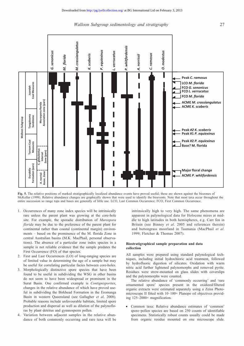
Fig. 5. The relative positions of marked stratigraphically localized abundance events have proved useful; these are shown against the biozones of McKellar (1998). Relative abundance changes are graphically shown that were used to identify the bioevents. Note that most taxa occur throughout the entire succession so range tops and bases are generally of little use. LCO, Last Common Occurrence; FCO, First Common Occurrence.
at BG International Ltd on February 3, 2013http://pg.lyellcollection.org/Downloaded from
M. A. Martin et al.28
Initially slide logging was very slow due to a large amount of disseminated plant material obscuring the spores and pol-len. This was partially solved by sieving the kerogen residues at 20 µm to remove the plant material.
•• Rare ornamented spores: Relative abundance estimates of ‘rare ornamented spores’ are based on total counts of up to 100 identifiable specimens on two oxidized/filtered strews mounts. Due to intrinsic rarity and/or dilution by plant detri-tus, ornamented spores were (i) very time-consuming to locate and (ii) total yields often were less than 100 specimens.
Some spore–pollen showed apparent signs of strong thermal alteration (oxidized Thermal Alteration Index ~4–5; c. 3%Ro vitrinite reflectance). It is suggested that this may be due to nat-ural oxidative processes or wildfires, not geothermal activity (wildfires in a similar environment were reported by Nielsen et al. 2010). For a detailed discussion on the issue of the oxida-tion of plant material, see Diessel & Gammidge (1998).
Palynofloras were dominated by gymnosperm pollen, chiefly Araucariacites and undifferentiated Alisporites/ Falcisporites with lesser amounts of Callialasporites dampieri, and a morphologically highly variable complex of fern and liverwort/sphagnum moss spores, comprising Baculatisporites, Osmundacites and Verrucosisporites. Ornamented spores, including Retitriletes and Neoraistrickia, generally comprise less than 2% of the total spore–pollen count, although Retitriletes austroclavatidites dominates the ornamental spore population. The diversity of spore–pollen species in individual samples is low although the overall diversity of ‘rare ornamented spores’ recorded in each core-hole is much higher (up to 90 species). The diversity of ‘rare ornamented spores’ increases downhole and appears to reach a maximum in the Taroom Coal Measures and Durabilla Formation.
Biozonation
Dating was based on the distribution of zonal index species in the Perth (Filatoff 1975), Clarence-Morton (Burger 1994) and Surat (Price 1997; McKellar 1998) Basins. Partridge (2006) has revised the pan-Australian zonation of Mesozoic time by Helby et al. (1987) that was further updated by Monteil (2006).
Murospora florida, which occurs down to 611.95 m in the well 4 core-hole, demonstrates that the Juandah Coal Measures, Tangalooma Sandstone and the upper portion of the Taroom Coal Measures were deposited sometime during Middle Callovian–Kimmeridgian Murospora florida Association Zone time. By comparison with Gallagher et al. (2008) and Turner et al. (2009), the unconformity between the WSG and overlying Springbok Sandstone Formation may represent the Callovian–Oxfordian Argoland break-up unconformity at 155 Ma (latest Oxfordian). The lower portion of the Taroom Coal Measures was deposited during the early Callovian Contignisporites glebulentus Interval Zone. The lowest formation recognized in the three core-holes, the Durabilla Formation, is no older than the late Bathonian to earliest Callovian Middle Jurassic Aequitriradites norrissii Association Zone. These findings support the biozona-tion and its relationship to the WSG of McKellar (1998) from the Roma Shelf 100 km to the NW of the current study area.
Almost all of the taxa range throughout the study succession. However, there were many isolated abundance events of a num-ber of taxa that appeared sequentially in each well. The qualita-tively identified bioevents from the ornamented spore portion of the dataset within the studied succession are illustrated in Figure 5. Given the small study set available, we have not attempted to formally subdivide the existing biozones, particularly the Murospora florida Association Zone.
Biofacies analysis
Fuzzy c-means clustering (FCM) is a data analysis/classification method that identifies groups of samples with similar composi-tions. Fuzzy set theory allows for the possibility that a sample can have an association with multiple classes or clusters (Zadeh 1965) unlike the hard clustering methods commonly used in aca-demic palaeontology. This is an important feature for biostrati-graphical data analysis because such datasets often include samples that are transitional between two or more ‘pure’ faunal or floral assemblages. See Gary et al. (2009) for a full review of the biostratigraphical application of FCM.
table 2. Correlation-coefficient data for each taxon in the study in each of the three calculated FCM cluster ‘centres’
Nominated taxon per centre
Ret
itri
lete
s au
stra
locl
avat
idit
es
Tra
nsit
iona
l
Phl
ebop
teri
spor
ites
eq
uiex
inus
Aequitriradites norrisii −0.08 0.07 0.04Annulispora folliculosa 0.19 −0.07 −0.18Camarozonosporites ramosus 0.32 −0.09 −0.33
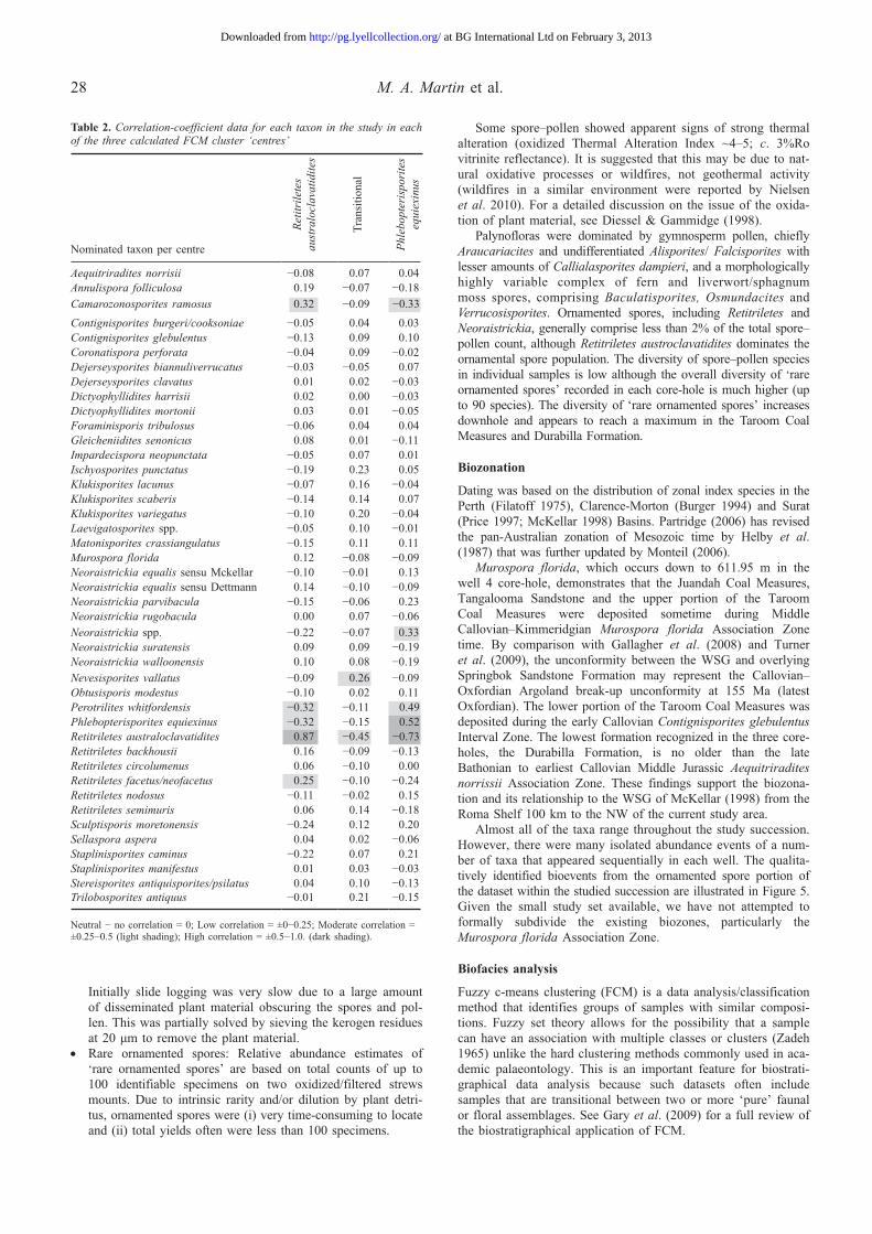
Contignisporites burgeri/cooksoniae −0.05 0.04 0.03Contignisporites glebulentus −0.13 0.09 0.10Coronatispora perforata −0.04 0.09 −0.02Dejerseysporites biannuliverrucatus −0.03 −0.05 0.07Dejerseysporites clavatus 0.01 0.02 −0.03Dictyophyllidites harrisii 0.02 0.00 −0.03Dictyophyllidites mortonii 0.03 0.01 −0.05Foraminisporis tribulosus −0.06 0.04 0.04Gleicheniidites senonicus 0.08 0.01 −0.11Impardecispora neopunctata −0.05 0.07 0.01Ischyosporites punctatus −0.19 0.23 0.05Klukisporites lacunus −0.07 0.16 −0.04Klukisporites scaberis −0.14 0.14 0.07Klukisporites variegatus −0.10 0.20 −0.04Laevigatosporites spp. −0.05 0.10 −0.01Matonisporites crassiangulatus −0.15 0.11 0.11Murospora florida 0.12 −0.08 −0.09Neoraistrickia equalis sensu Mckellar −0.10 −0.01 0.13Neoraistrickia equalis sensu Dettmann 0.14 −0.10 −0.09Neoraistrickia parvibacula −0.15 −0.06 0.23Neoraistrickia rugobacula 0.00 0.07 −0.06Neoraistrickia spp. −0.22 −0.07 0.33 Neoraistrickia suratensis 0.09 0.09 −0.19Neoraistrickia walloonensis 0.10 0.08 −0.19Nevesisporites vallatus −0.09 0.26 −0.09Obtusisporis modestus −0.10 0.02 0.11Perotrilites whitfordensis −0.32 −0.11 0.49 Phlebopterisporites equiexinus −0.32 −0.15 0.52 Retitriletes australoclavatidites 0.87 −0.45 −0.73 Retitriletes backhousii 0.16 −0.09 −0.13Retitriletes circolumenus 0.06 −0.10 0.00Retitriletes facetus/neofacetus 0.25 −0.10 −0.24Retitriletes nodosus −0.11 −0.02 0.15Retitriletes semimuris 0.06 0.14 −0.18Sculptisporis moretonensis −0.24 0.12 0.20Sellaspora aspera 0.04 0.02 −0.06Staplinisporites caminus −0.22 0.07 0.21Staplinisporites manifestus 0.01 0.03 −0.03Stereisporites antiquisporites/psilatus 0.04 0.10 −0.13Trilobosporites antiquus −0.01 0.21 −0.15
Neutral − no correlation = 0; Low correlation = ±0−0.25; Moderate correlation = ±0.25−0.5 (light shading); High correlation = ±0.5−1.0. (dark shading).
at BG International Ltd on February 3, 2013http://pg.lyellcollection.org/Downloaded from
Walloon Subgroup sedimentology and stratigraphy 29
Fuzzy c-means clustering was implemented using the FCM module, provided as part of the biostratigraphical data analysis software package TACSWorks. TACSWorks was developed by the Technical Alliance for Computational Stratigraphy (TACS) at the University of Utah and was used to accomplish the following tasks:
1. determine the appropriate number of clusters;2. resolve cluster ‘centres’ and memberships;3. rank species based on correlation to each cluster, to evaluate
the suitability and utility of index species;4. visualize cluster ‘centres’ as faunal/floral assemblage bar graphs;5. visualize cluster memberships as downhole assemblage curves.
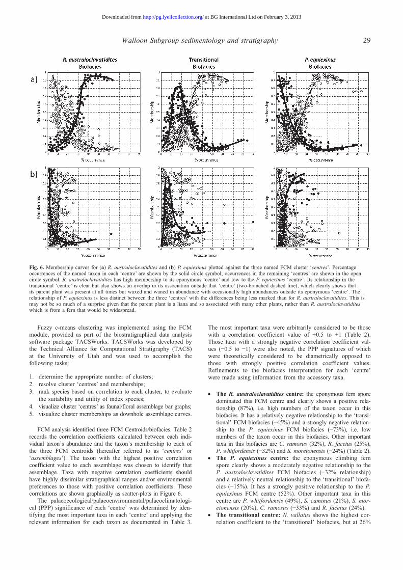
FCM analysis identified three FCM Centroids/biofacies. Table 2 records the correlation coefficients calculated between each indi-vidual taxon’s abundance and the taxon’s membership to each of the three FCM centroids (hereafter referred to as ‘centres’ or ‘assemblages’). The taxon with the highest positive correlation coefficient value to each assemblage was chosen to identify that assemblage. Taxa with negative correlation coefficients should have highly dissimilar stratigraphical ranges and/or environmental preferences to those with positive correlation coefficients. These correlations are shown graphically as scatter-plots in Figure 6.
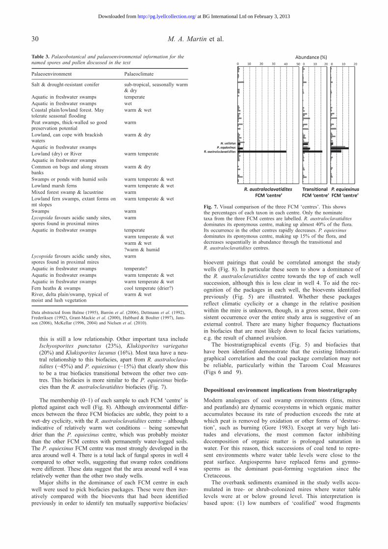
The palaeoecological/palaeoenvironmental/palaeoclimatologi-cal (PPP) significance of each ‘centre’ was determined by iden-tifying the most important taxa in each ‘centre’ and applying the relevant information for each taxon as documented in Table 3.
The most important taxa were arbitrarily considered to be those with a correlation coefficient value of +0.5 to +1 (Table 2). Those taxa with a strongly negative correlation coefficient val-ues (−0.5 to −1) were also noted, the PPP signatures of which were theoretically considered to be diametrically opposed to those with strongly positive correlation coefficient values. Refinements to the biofacies interpretation for each ‘centre’ were made using information from the accessory taxa.
•• the R. australoclavatidites centre: the eponymous fern spore dominated this FCM centre and clearly shows a positive rela-tionship (87%), i.e. high numbers of the taxon occur in this biofacies. It has a relatively negative relationship to the ‘transi-tional’ FCM biofacies (−45%) and a strongly negative relation-ship to the P. equiexinus FCM biofacies (−73%), i.e. low numbers of the taxon occur in this biofacies. Other important taxa in this biofacies are C. ramosus (32%), R. facetus (25%), P. whitfordensis (−32%) and S. moretonensis (−24%) (Table 2).
•• the P. equiexinus centre: the eponymous climbing fern spore clearly shows a moderately negative relationship to the P. australoclavatidites FCM biofacies (−32% relationship) and a relatively neutral relationship to the ‘transitional’ biofa-cies (−15%). It has a strongly positive relationship to the P. equiexinus FCM centre (52%). Other important taxa in this centre are P. whitfordensis (49%), S. caminus (21%), S. mor-etonensis (20%), C. ramosus (−33%) and R. facetus (24%).
•• the transitional centre: N. vallatus shows the highest cor-relation coefficient to the ‘transitional’ biofacies, but at 26%
Fig. 6. Membership curves for (a) R. australoclavatidites and (b) P. equiexinus plotted against the three named FCM cluster ‘centres’. Percentage occurrences of the named taxon in each ‘centre’ are shown by the solid circle symbol; occurrences in the remaining ‘centres’ are shown in the open circle symbol. R. australoclavatidites has high membership to its eponymous ‘centre’ and low to the P. equiexinus ‘centre’. Its relationship in the transitional ‘centre’ is clear but also shows an overlap in its association outside that ‘centre’ (two-branched dashed line), which clearly shows that its parent plant was present at all times but waxed and waned in abundance with occasionally high abundances outside its eponymous ‘centre’. The relationship of P. equiexinus is less distinct between the three ‘centres’ with the differences being less marked than for R. australoclavatidites. This is may not be so much of a surprise given that the parent plant is a liana and so associated with many other plants, rather than R. australoclavatidites which is from a fern that would be widespread.
at BG International Ltd on February 3, 2013http://pg.lyellcollection.org/Downloaded from
M. A. Martin et al.30
this is still a low relationship. Other important taxa include Ischyosporites punctatus (23%), Klukisporites variegatus (20%) and Klukisporites lacunus (16%). Most taxa have a neu-tral relationship to this biofacies, apart from R. australoclava-tidites (−45%) and P. equiexinus (−15%) that clearly show this to be a true biofacies transitional between the other two cen-tres. This biofacies is more similar to the P. equiexinus biofa-cies than the R. australoclavatidites biofacies (Fig. 7).
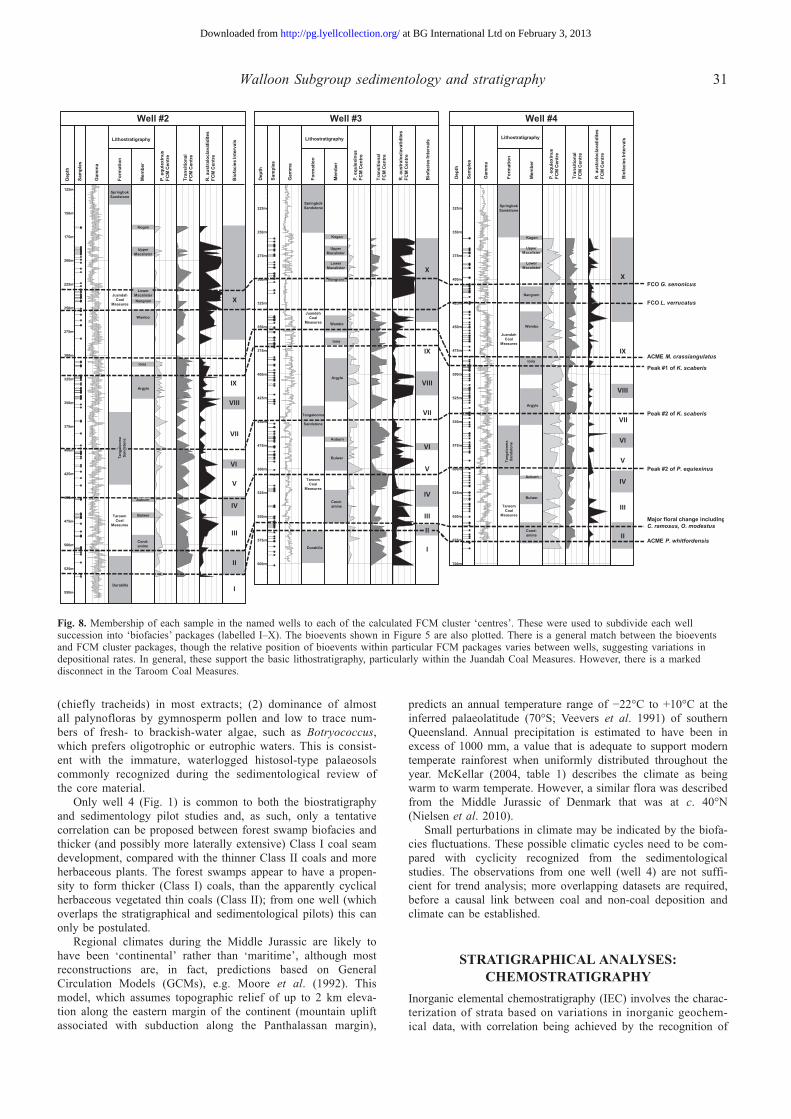
The membership (0–1) of each sample to each FCM ‘centre’ is plotted against each well (Fig. 8). Although environmental differ-ences between the three FCM biofacies are subtle, they point to a wet–dry cyclicity, with the R. australoclavatidites centre – although indicative of relatively warm wet conditions – being somewhat drier than the P. equiexinus centre, which was probably moister than the other FCM centres with permanently water-logged soils. The P. equiexinus FCM centre was most strongly developed in the area around well 4. There is a total lack of fungal spores in well 4 compared to other wells, sug gesting that swamp redox conditions were different. These data suggest that the area around well 4 was relatively wetter than the other two study wells.
Major shifts in the dominance of each FCM centre in each well were used to pick biofacies packages. These were then iter-atively compared with the bioevents that had been identified previously in order to identify ten mutually supportive biofacies/
bioevent pairings that could be correlated amongst the study wells (Fig. 8). In particular these seem to show a dominance of the R. australoclavatidites centre towards the top of each well succession, although this is less clear in well 4. To aid the rec-ognition of the packages in each well, the bioevents identified previously (Fig. 5) are illustrated. Whether these packages reflect climatic cyclicity or a change in the relative position within the mire is unknown, though, in a gross sense, their con-sistent occurrence over the entire study area is suggestive of an external control. There are many higher frequency fluctuations in biofacies that are most likely down to local facies variations, e.g. the result of channel avulsion.
The biostratigraphical events (Fig. 5) and biofacies that have been identified demonstrate that the existing lithostrati-graphical correlation and the coal package correlation may not be reliable, particularly within the Taroom Coal Measures (Figs 6 and 9).
depositional environment implications from biostratigraphy
Modern analogues of coal swamp environments (fens, mires and peatlands) are dynamic ecosystems in which organic matter accumulates because its rate of production exceeds the rate at which peat is removed by oxidation or other forms of ‘destruc-tion’, such as burning (Gore 1983). Except at very high lati-tudes and elevations, the most common factor inhibiting decomposition of organic matter is prolonged saturation in water. For this reason, thick successions of coal tend to repre-sent environments where water table levels were close to the peat surface. Angiosperms have replaced ferns and gymno-sperms as the dominant peat-forming vegetation since the Cretaceous.
The overbank sediments examined in the study wells accu-mulated in tree- or shrub-colonized mires where water table levels were at or below ground level. This interpretation is based upon: (1) low numbers of ‘coalified’ wood fragments
table 3. Palaeobotanical and palaeoenvironmental information for the named spores and pollen discussed in the text
Palaeoenvironment Palaeoclimate
Salt & drought-resistant conifer sub-tropical, seasonally warm & dry
Aquatic in freshwater swamps temperateAquatic in freshwater swamps wetCoastal plain/lowland forest. May tolerate seasonal flooding
warm & wet
Peat swamps, thick-walled so good preservation potential
warm
Lowland, can cope with brackish waters
warm & dry
Aquatic in freshwater swamps Lowland (dry) or River warm temperateAquatic in freshwater swamps Common on bogs and along stream banks
warm & dry
Swamps or ponds with humid soils warm temperate & wetLowland marsh ferns warm temperate & wetMixed forest swamp & lacustrine warmLowland fern swamps, extant forms on mt slopes
warm temperate & wet
Swamps warmLycopsida favours acidic sandy sites, spores found in proximal mires
warm
Aquatic in freshwater swamps temperate warm temperate & wet warm & wet ?warm & humidLycopsida favours acidic sandy sites, spores found in proximal mires
warm
Aquatic in freshwater swamps temperate?Aquatic in freshwater swamps warm temperate & wetAquatic in freshwater swamps warm temperate & wetFern heaths & swamps cool temperate (drier?)River, delta plain/swamp, typical of moist and lush vegetation
warm & wet
Data abstracted from Balme (1995), Barrón et al. (2006), Dettmann et al. (1992), Frederiksen (1992), Grant-Mackie et al. (2000), Hubbard & Boulter (1997), Jans-son (2006), McKellar (1996, 2004) and Nielsen et al. (2010).
Fig. 7. Visual comparison of the three FCM ‘centres’. This shows the percentages of each taxon in each centre. Only the nominate taxa from the three FCM centres are labelled. R. australoclavatidites dominates its eponymous centre, making up almost 40% of the flora. Its occurrence in the other centres rapidly decreases. P. equiexinus dominates its eponymous centre, making up 15% of the flora, and decreases sequentially in abundance through the transitional and R. australoclavatidites centres.
at BG International Ltd on February 3, 2013http://pg.lyellcollection.org/Downloaded from
Walloon Subgroup sedimentology and stratigraphy 31
(chiefly tracheids) in most extracts; (2) dominance of almost all palynofloras by gymnosperm pollen and low to trace num-bers of fresh- to brackish-water algae, such as Botryococcus, which prefers oligotrophic or eutrophic waters. This is consist-ent with the immature, waterlogged histosol-type palaeosols commonly recognized during the sedimentological review of the core material.
Only well 4 (Fig. 1) is common to both the biostratigraphy and sedimentology pilot studies and, as such, only a tentative correlation can be proposed between forest swamp biofacies and thicker (and possibly more laterally extensive) Class I coal seam development, compared with the thinner Class II coals and more herbaceous plants. The forest swamps appear to have a propen-sity to form thicker (Class I) coals, than the apparently cyclical herbaceous vegetated thin coals (Class II); from one well (which overlaps the stratigraphical and sedimentological pilots) this can only be postulated.
Regional climates during the Middle Jurassic are likely to have been ‘continental’ rather than ‘maritime’, although most reconstructions are, in fact, predictions based on General Circulation Models (GCMs), e.g. Moore et al. (1992). This model, which assumes topographic relief of up to 2 km eleva-tion along the eastern margin of the continent (mountain uplift associated with subduction along the Panthalassan margin),
predicts an annual temperature range of −22°C to +10°C at the inferred palaeolatitude (70°S; Veevers et al. 1991) of southern Queensland. Annual precipitation is estimated to have been in excess of 1000 mm, a value that is adequate to support modern temperate rainforest when uniformly distributed throughout the year. McKellar (2004, table 1) describes the climate as being warm to warm temperate. However, a similar flora was described from the Middle Jurassic of Denmark that was at c. 40°N (Nielsen et al. 2010).
Small perturbations in climate may be indicated by the biofa-cies fluctuations. These possible climatic cycles need to be com-pared with cyclicity recognized from the sedimentological studies. The observations from one well (well 4) are not suffi-cient for trend analysis; more overlapping datasets are required, before a causal link between coal and non-coal deposition and climate can be established.
StrAtIGrAPHIcAl AnAlySES: cHEMoStrAtIGrAPHy
Inorganic elemental chemostratigraphy (IEC) involves the charac-terization of strata based on variations in inorganic geochem-ical data, with correlation being achieved by the recognition of
325m
350m
375m
400m
425m
450m
475m
500m
525m
550m
575m
600m
625m
650m
675m
700m
SpringbokSandstone
Dep
th
Sam
ples
Gam
ma
Lithostratigraphy
Form
atio
n
Mem
ber
P. e
quie
xinu
sFC
M C
entr
e
Tran
sitio
nal
FCM
Cen
tre
R. a
ustr
aloc
lava
tidite
sFC
MC
ent
Bio
faci
esIn
terv
als
II
III
IV
V
VI
VII
VIII
IX
X
Auburn
Bulwer
Cond-amine
Tang
aloo
ma
Sand
ston
eTaroom
CoalMeasures
JuandahCoal
Measures
Kogan
UpperMacalister
LowerMacalister
Nangram
Wambo
Iona
Argyle
125m
150m
175m
200m
225m
250m
275m
300m
325m
350m
375m
400m
425m
450m
475m
500m
525m
550m
SpringbokSandstone
Durabilla
TaroomCoal
Measures
Kogan
Nangram
Wambo
Iona
Argyle
Bulwer
Cond-amine
I
II
III
IV
VI
VII
VIII
V
IX
X Juandah
CoalMeasures
Dep
th
Sam
ples
Gam
ma
Lithostratigraphy
Form
atio
n
Mem
ber
P. e
quie
xinu
sFC
M C
entr
e
Tran
sitio
nal
FCM
Cen
tre
R. a
ustr
aloc
lava
tidite
sFC
M C
entr
e
Bio
faci
esIn
terv
als
225m
250m
275m
300m
325m
350m
375m
400m
425m
450m
475m
500m
525m
550m
575m
600m
SpringbokSandstone
Durabilla
JuandahCoal
Measures
Tangalooma
Sandstone
Auburn
Bulwer
Cond-amine
TaroomCoal
Measures
Kogan
UpperMacalister
LowerMacalister
Wambo
Iona
Argyle
Dep
th
Sam
ples
Gam
ma
Lithostratigraphy
Form
atio
n
Mem
ber
P. e
quie
xinu
sFC
M C
entr
e
Tran
sitio
nal
FCM
Cen
tre
R. a
ustr
aloc
lava
tidite
sFC
M C
entr
e
Bio
faci
esIn
terv
als
I
III
IV
VII
VIII
V
IX
X
VI
II
Well #2 Well #3 Well #4
Nangram
Tang
aloo
ma
Sand
ston
e
Auburn
UpperMacalister
LowerMacalister
FCO G. senonicus
FCO L. verrucatus
ACME M. crassiangulatus
Major floral change includingC. ramosus, O. modestus
ACME P. whitfordensis
Peak #2 of P. equiexinus
Peak #2 of K. scaberis
Peak #1 of K. scaberis
re
Fig. 8. Membership of each sample in the named wells to each of the calculated FCM cluster ‘centres’. These were used to subdivide each well succession into ‘biofacies’ packages (labelled I–X). The bioevents shown in Figure 5 are also plotted. There is a general match between the bioevents and FCM cluster packages, though the relative position of bioevents within particular FCM packages varies between wells, suggesting variations in depositional rates. In general, these support the basic lithostratigraphy, particularly within the Juandah Coal Measures. However, there is a marked disconnect in the Taroom Coal Measures.
at BG International Ltd on February 3, 2013http://pg.lyellcollection.org/Downloaded from
M. A. Martin et al.32
compared geochemical signatures in adjacent sections or wells (Jarvis & Jarvis 1992a, b; Pearce et al. 2010). IEC is routinely used within the petroleum industry due to large datasets being acquired from small sample volumes either within the laboratory or at wellsite. The technique has proved successful in detecting and correlating geochemical variation when dealing with appar-ently uniform lithological and barren or virtually barren succes-sions. Consequently, reservoir correlations and stratigraphical picks can be established with confidence, even for those succes-sions over which the electric-log traces show little significant change.
IEC has been utilized previously within the Surat and Bowen basins (Andrew et al. 1996), where conventional tech-niques, such as lithostratigraphical, wireline and biostratigraph-ical analysis, failed to distinguish between the Triassic Rewan and Showground formations for the purpose of petroleum exploration.
Geochemical analysis was undertaken on 345 core samples; mostly silty claystones, along with some coal/argillaceous coal samples, plus a few samples from sandstones, tuffs and palaeo-sols. Following powdering in a swing mill grinder, the core
samples were subjected to geochemical analysis by open acid digestion and micro-fusion techniques on 0.1 g of material fol-lowed by an ICP-OES and ICP-MS analysis, with data being acquired for 47 elements.
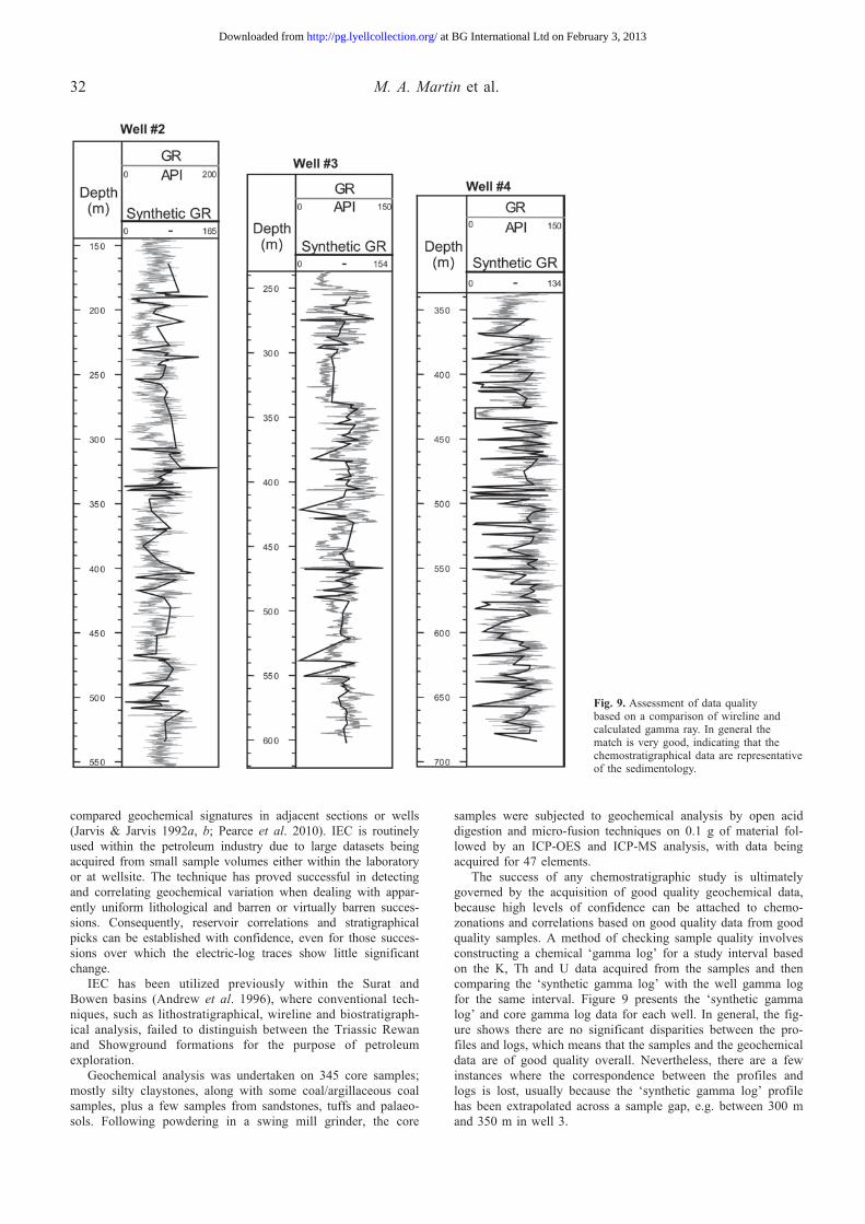
The success of any chemostratigraphic study is ultimately governed by the acquisition of good quality geochemical data, because high levels of confidence can be attached to chemo-zonations and correlations based on good quality data from good quality samples. A method of checking sample quality involves constructing a chemical ‘gamma log’ for a study interval based on the K, Th and U data acquired from the samples and then comparing the ‘synthetic gamma log’ with the well gamma log for the same interval. Figure 9 presents the ‘synthetic gamma log’ and core gamma log data for each well. In general, the fig-ure shows there are no significant disparities between the pro-files and logs, which means that the samples and the geochemical data are of good quality overall. Nevertheless, there are a few instances where the correspondence between the profiles and logs is lost, usually because the ‘synthetic gamma log’ profile has been extrapolated across a sample gap, e.g. between 300 m and 350 m in well 3.
Fig. 9. Assessment of data quality based on a comparison of wireline and calculated gamma ray. In general the match is very good, indicating that the chemostratigraphical data are representative of the sedimentology.
at BG International Ltd on February 3, 2013http://pg.lyellcollection.org/Downloaded from
Walloon Subgroup sedimentology and stratigraphy 33
Geochemistry, mineralogy and lithology
Chemostratigraphy can be employed to characterize intervals of sedimentary rocks by using inorganic geochemical data typically acquired by ICP analyses. Usually, however, the data for only a limited number of ‘key’ elements are sufficiently distinctive to characterize a sedimentary rock interval and give it what is termed a geochemical ‘fingerprint’. In this study elements have been combined as ‘key element ratios’, the changing up-succes-sion values of which add further detail to the geochemical char-acterization of sedimentary rock intervals. However, the elements utilized as key elements and combined as key element ratios vary between geographical areas and stratigraphic intervals due to dif-ferences in detrital mineralogy and provenance composition: the mineralogy and geochemistry of different source areas can vary
considerably, which therefore influences the geochemistry of the sediments derived from these areas. Under different diagenetic regimes, including weathering, many elements may become remobilized, resulting in the detritalsignatures of the sediments becoming either modified or obliterated. A comprehensive review of the factors controlling the geochemistry of the WSG as pene-trated by the three study wells has not been carried out.
Establishing the mineral affinities of the key elements with as much confidence as possible is important, the best way to do so is by a comparison of mineralogical and geochemical data from the same samples. Unfortunately, mineralogical data are not available for the current study, so Principal Component Analysis (PCA) was applied to the geochemical data in order to recognize element associations, from which the likely mineral affinity of these elements can be inferred.
CaO
Sr
Na2O
P2O5
Mo
Cr
Ni
V TlK2O
Zn
Fe2O3
Rb
ScBa
Cu
MnO
Si2O2
HREE’s
Y LREE’s
MREE’s
Li
Al2O3
Sn
TiO2
Hf
Th
U
Nb
Co
MgO
Pb Ta
Zr
0.2
0.1
0
-0.1
-0.2
0.3
0.4 0.5 -0.3
-0.4
EV2
EV3
Group 1 Tuffaceous
Group 2 Tuffaceous
0.2 0.1 0 -0.1-0.2 0.3-0.3
Cs
0.1
0
-0.1-0.2 0.3 0 0.1 0.2
EV1
EV2
Sr
Ni
V
Sc
Zn
Ba
Y
LREE’s
MREE’s
Pb
Sn
Hf Th
Nb
P2O5
Mo
Co
HREE’s
CaO
MnO
TiO2
Cs
K2O
Si2O2
MgO
Li
Zr
Group 1 Tuffaceous
Group 2 Tuffaceous
Group 3 Carbonate Minerals
U
0.2 Cu
Na2O
Rb
Cr
Fe2O3
Tl
Group 4 Clay Minerals
Y
LREE’s MREE’s
Li Al2O3
Pb
TaSn
Co
0.2
0.1
0
-0.1
-0.2
0.3
0.4
0.5
-0.3-0.4
EV3
EV4
0.2 0.1 0 -0.1-0.2 0.3 0.4 0.5
Group 2 Tuffaceous
Group 3 Carbonate
Minerals
Uncertain affinity
Fe2O3
TiO2
Sc
Cs
Cr
NiV
SrTl
K2O
Ba
Cu
Si2O2
Hf
Th
U
Zr Nb
P2O5
CaOMnO
HREE’s
MgO
Zn
Na2O
Mo
0.2
0.1
0
-0.1
-0.2
0.3
0.4
EV1
EV2
Cs
Rb
Ni
V
Sc
Sr
Tl
K2O
Zn
Ba
Cu
SiO2
LREE’s
MREE’s
Li
Al2O3
Pb
Ta
Sn
Hf
Th
U
Zr
P2O5
MnO
Co
Group 4 Clay Minerals Group 2
TuffaceousType 2
Group 1 TuffaceousType 1
Group 3 CarbonateMinerals
0.2 0.1 0 -0.1-0.2 0.3 0.4
TiO2
HREE’sY
Nb
Mo
CaO
Fe2O3
MgO
Na2O
0.2
0.1
0
-0.1
-0.2
0.3
0.4
EV2
EV3
Silt-grade Material
Cs
Rb
Cr
Ni
V
Sc
SrTl
K2O
Zn
Na2O
Cu
SiO2
Y
LREE’s
MREE’s
Li
Al2O3
Pb
Ta
Zr
TiO2
Hf
Th
U
Nb
P2O5
Mo
Co
0.2 0.1 0 -0.1-0.2 0.3 0.4
HREE’s
Fe2O3
CaO
Sn
MgO
MnO
0.2
0.1
0
-0.1
-0.2
0.3
0.4
-0.3
EV3
EV4
?Chlorite
Cs
RbCr
Ni
V Sc
Sr
Tl
Zn
Ba
Cu
SiO2
Y LREE’s MREE’s
Li
Al2O3 Pb
Ta
Sn
TiO2
Hf
Th
U
Zr
Nb
P2O5
Mo
Co
0.2 0.1 0 -0.1-0.2 0.3 0.4
HREE’s
Na2O
K2O
Fe2O3
MgOCaO
MnO
Quartz Zircon
Plagioclase
Apatite
A D
B E
C F
Tuffaceous
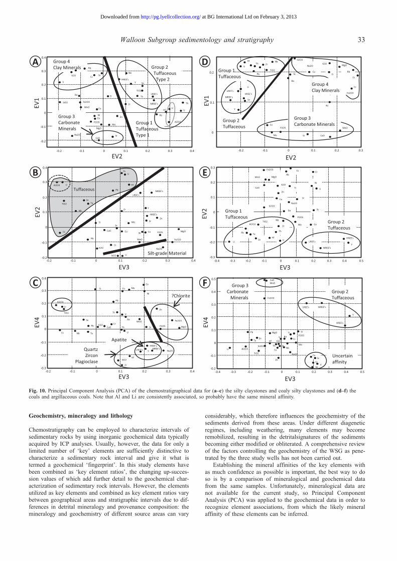
Fig. 10. Principal Component Analysis (PCA) of the chemostratigraphical data for (a–c) the silty claystones and coaly silty claystones and (d–f) the coals and argillaceous coals. Note that Al and Li are consistently associated, so probably have the same mineral affinity.
at BG International Ltd on February 3, 2013http://pg.lyellcollection.org/Downloaded from
M. A. Martin et al.34
Principal component Analysis
PCA is a statistical technique used to identify important associa-tions. Elements clustering together in the same area of an eigen-vector plot are likely to have similar mineral affinities. The principal component scores for the original vectors (eigenvectors) indicate the association of certain elements and the relationship between some elements and mineralogy/lithology. Prior to PCA being undertaken the selected samples were classified into broad geochemical lithotypes, using the following characteristics:
•• silty claystones/claystones; Si/Al (proxy for quartz: clay con-tents) values below 5;
•• coaly silty claystones; Si/Al values below 5 and LOI (Loss on Ignition) values <50%;
•• argillaceous coals; LOI values from 50–70%;•• coals; LOI values >70%.
PCA is first applied to the silty claystones and subsequently to the coals, argillaceous coals and coaly silty claystones. The aim of these tests is to establish any lithological affinities the various elements might have.
From this point on, the major element oxides are represented by just their chemical symbols, e.g. K for K2O, Al for Al2O3, Si for SiO2, and so forth. The rare earth elements (REE) are grouped for the PCA into light rare earth elements (LREE) – La, Ce and Pr; medium rare earth elements (MREE) – Nd, Sm, Eu, Gd, Dy and Ho; and heavy rare earth elements (HREE) – Er, Tm, Yb and Lu.
PcA results: silty claystones/coaly silty claystones
Eigenvectors EV1: EV2. EV1 and EV2 together represent 49% of the total variance of the silty claystone/coaly silty claystone geo-chemical dataset. When the EV1 and EV2 values for the various elements are plotted against one another, several broad element associations can be recognized (see Fig. 10a), as follows:
•• Group 1: includes Li, Al, Th, U, Hf and Pb, and is character-ized by +ve EV2 values and −ve to +ve EV1 values. The con-centrations of these elements is controlled by the abundance and distribution not only of those minerals occurring in volcanic ash, but also of glass shards found in volcanic ashes which are similar to the bentonites found in Southern Queensland. However, high Al concentrations reflect the presence of kaolin-ite, which is an alteration product of the tuffaceous material.
•• Group 2: includes Nb, Y, Sn, Ti, Ta and the REE, and is characterized by +ve EV1 values and +ve EV2 values. These elements are associated with the minerals, such as smectites, found in intermediate volcanic ashes.
•• Group 3: includes Ca and Sr and is characterized by −ve EV1 values and +ve to −ve EV2 values – both elements have an affinity with carbonate minerals. Moreover, Figure 10a shows P, Mg and Mo plot close to Ca and Sr, which indi-cates they may be, in part, linked to carbonate minerals.
•• Group 4: includes V, K, Cr, Rb, Cs and Sc, and is charac-terized by +ve EV1 values and −ve EV2 values. These ele-ments are believed to be linked to clay minerals and to illite+mica in particular, as well as to K feldspar.
Eigenvectors EV2: EV3. EV2 and EV3 are plotted to highlight any subtle variations in minerals affinities and together represent 25% of the total variance of the silty claystone/coaly silty clay-stone geochemical dataset. When the EV2 and EV3 values for the various elements are plotted against one another, two broad element associations can be identified (see Fig. 10b), as follows:
•• Group 1: includes Li, Al and Ti (grey shaded area), and is characterized by +ve to −ve EV3 values and +ve EV2
values. The concentrations of these elements are governed by the abundance and distribution of those minerals found in volcanic ash, such as orthopyroxene and plagioclase.
•• Group 2: includes Si and Na (below the sand line) and is characterized by +ve EV3 values and −ve EV2 values. Si is strongly associated with quartz, whereas Na is linked with plagioclase – both minerals probably occur in the form of silt-grade grains in the silty claystones.
Eigenvectors EV3: EV4. EV3 and EV4 are also plotted to high-light any subtle variations in mineral affinities and together repre-sent 16% of the total variance of the silty claystone/coaly silty claystone geochemical dataset. When the EV3 and EV4 values for the various elements are plotted against one another, two broad element associations can be identified (see Fig. 10c), as follows:
•• Group 1: includes Zn, P, Fe and Mg, and is characterized by +ve EV3 values and +ve EV4 values. The abundance of these elements is believed to be controlled by the abundance and distribution of chloritic minerals.
•• Group 2: includes Na, Si, Y, Zr, Hf and the REEs, and is characterized by −ve EV4 values and +ve EV3 values. These elements have affinities with quartz, plagioclase, zircon and possibly apatite, all of which are found in the form of silt-grade grains in the silty claystones. This composition is attributed to the background detrital provenance signal of the WSG that is probably more prevalent in sandstones.
PcA results: coals/argillaceous coals
Eigenvectors EV1: EV2. EV1 and EV2 together represent 50% of the total variance of the combined geochemical dataset relating to the coals and argillaceous coals. When the EV1 and EV2 values for the various elements are plotted against one another, several broad element associations can be recognized as follows (see Fig. 10d):
•• Group 1: includes U, Hf, Ta, Th, Zr, Nb, Pb, Al and Ti and is characterized by +ve EV1 values and −ve EV2 values. The con-centrations of these elements are controlled by the abundance and distribution not only of those minerals occurring in volcanic ash but also of glass shards within the tuffaceous material.
•• Group 2: includes Li, Y, Sn and the REEs. The group is characterized by +ve EV1 values and −ve EV2 values and is attributed to the distribution of a subordinate and discrete composition of volcanic ash minerals/glass shards similar to those that developed in Group 1.
•• Group 3: includes Ca, Sr, Co, Mo, P and Mn, and is charac-terized by +ve to −ve EV1 values and +ve to −ve EV2 val-ues. These elements are associated with carbonate minerals and siderite.
•• Group 4: includes Na, K, Rb and Cs, and is characterized by +ve EV1 values and +ve EV2 values. The above elements have affinities with clay minerals.
Eigenvectors EV2: EV3. EV2 and EV3 together represent 17% of the total variance of the combined geochemical dataset relating to the coals and argillaceous coals. When the EV2 and EV3 values for the various elements are plotted against one another, two broad element associations can be identified (see Fig. 10e), as follows:
•• Group 1: includes Li, Al, Sn and Ti, and is characterized by +ve to −ve EV3 values and −ve EV2 values. The concentra-tions of these elements are governed by the abundance and distribution of those minerals found in volcanic ash.
•• Group 2: includes the REEs and Y and is characterized by +ve EV3 values and −ve EV2 values. The REEs and Y have affinities with tuffaceous material.
at BG International Ltd on February 3, 2013http://pg.lyellcollection.org/Downloaded from
Walloon Subgroup sedimentology and stratigraphy 35
Eigenvectors EV3: EV4. EV3 and EV4 together represent 14% of the total variance of the combined geochemical dataset relat-ing to the coals and argillaceous coals. When the EV3 and EV4 values for the various elements are plotted against one another, two broad element associations can be identified (see Fig. 10f), as follows:
•• Group 2: includes the REEs and Y and is characterized by +ve EV3 values and +ve EV4 values. The abundance of these elements is governed by the abundance and distribution of tuffaceous material.
•• Group 3: includes Ca and Mn and is characterized by −ve EV3 values and high +ve EV4 values. Both elements have affinities with carbonate minerals.
Summary of the element to mineral affinities
Based on the PCA results the following element–mineral affini-ties relate to the silty claystones and coals of the WSG.
•• Si and Na = quartz and plagioclase, but sometimes both ele-ments are also associated with other detrital minerals found in siliciclastic rocks.
•• Al, Li, Hf, U, Th, Nb, Ta, Ti, Sn and the REEs = in the silty claystones and coals, these elements are primarily asso-ciated with tuffaceous material. However, the PCA results suggest that the composition of the tuffaceous material is variable, with some samples containing tuffaceous material with high levels of Al, U and Li, while other samples con-tain tuffaceous material with high levels of Ti, Nb, Ta, Sn and REEs.
•• K, Rb, Cs, Ga, Sc and Cr = clay minerals, and illite+mica in particular, though to a lesser degree, K and Rb are linked to feldspar.
•• Fe, Ni, Co, Zn and V = the mineral affinities of these ele-ments in the WSG are difficult to establish with certainty, though overall, they probably are most likely to be associated with grain-coating and pore-filling minerals, such as haema-tite. However, Fe also has an affinity with siderite when locally associated with Mn and may also be linked with minor amounts of chlorite and pyrite. Sideritic horizons and nodules have been recognized in each of the wells, which are evident when plotted as a Fe/Mn ratio.
•• Ca, Mn, Mg and Sr = carbonate minerals, of which calcite, dolomite and siderite are the most important. These elements may also have affinities with smectitic and chloritic clay minerals when associated with Al.
•• P = phosphate, clay and carbonate minerals•• Zr, Hf, Th, Y and U = zircon. The presence of abundant zir-
con will also influence the concentrations of Th, U and the HREEs, as these elements occur in this heavy mineral. In addition, Hf, Th, Y and U levels tend to be relatively high in tuffaceous material.
•• Co, Ni, Zn, V can also have an affinity along with Cu to clay minerals and mica. These elements are also linked with organic material – they are released during oxidation of this material, becoming remobilized during diagenesis. Ni is also associated with Fe–sulfide minerals.
cHEMoStrAtIGrAPHIc ZonAtIon oF tHE Study WEllS
Geochemical profiles covering the three study wells were con-structed for selected key element ratios (Fig. 11). Based on the changing up-succession morphology of these profiles over the study intervals, the study intervals can be divided into nine geochemically
distinct divisions, termed chemostratigraphical packages (CM). Recognition of these packages is based on up-succession changes in the values of the key element ratios: Sc/Nb, Fe/Mn, K/Rb (log values), Nb/Ti and Mg/Ca. The mineralogical significance of these key element ratios is as follows:
•• Sc/Rb values – kaolinite abundance relative to illite+mica abundance;
•• K/Rb values – K feldspar abundance relative to illite+mica abundance;
•• Nb/Ti values – variations in the abundance of volcanic ash;•• Mg/Ca values – variations in the composition of the carbon-
ate minerals;•• Fe/Mn values – the abundance of chloritic clay minerals rela-
tive to the abundance of carbonate minerals, and siderite in particular.
The values of the above ratios are ultimately controlled by the interplay between changes in provenance, climate and deposi-tional environment. Furthermore, silty claystone geochemistry is also influenced by how much tuffaceous material is present and its geochemical composition. The chemostratigraphical packages are shown in Figure 11.
With more widely spaced wells it might be possible to iden-tify thickness trends in the volcanic material and thus elucidate a source direction.
coMPArISon oF tHE cHEMoZonAtIon And BIoStrAtIGrAPHIcAl EvEntS
The chemostratigraphical study provided an independent strati-graphical correlation and presented below is a comparison between the bioevents and the chemostratigraphical zonations, to determine if any of the events consistently occur at the same horizons within the chemostratigraphic zonations. The results are illustrated in Figure 11.
•• CM-1 is present within wells 2 and 3, and may lie below the current sample interval within well 4. The ACME of P. whit-fordensis is present within the top of CM-1 in well 2; how-ever, it is present within the lowermost part of CM-2 within wells 3 and 4. This may be due to data closure issues or edge-effects with both the chemostratigraphical and biostrati-graphical datasets.
•• CM-2 is present in all wells and contains the major down-hole floristic change highlighted by the marked abundance increases of C. ramosus, O. modestus, A. norrissii and P. whitfordensis. This ties to the top of Biofacies II.
•• CM-3, like CM-2, is present in all three wells and consist-ently contains the lowermost abundance ‘event’ of P. equiex-inus. The top of Biofacies IV occurs in the lowermost part of CM-3 but does not always coincide with the P. equiexinus bioevent.
•• No Bioevents are recorded within CM-4, although Biofacies VI appears in the middle of the package.
•• The top and base of CM-5 corresponds to Peaks 1 and 2 of K. scaberis.
•• The ACME of M. crassiangulatus is consistently seen in the lowermost part of CM-6. The major upward drying, as indicated by Biofacies X, generally starts in CM-6 apart from in well 4, which appears to have been deposited in a wetter environment anyway.
•• CM-7 contains the FCO of L. verrucatus and the FCO of G. senonicus, respectively, although their positions within the package vary considerably, probably as a result of variable
at BG International Ltd on February 3, 2013http://pg.lyellcollection.org/Downloaded from
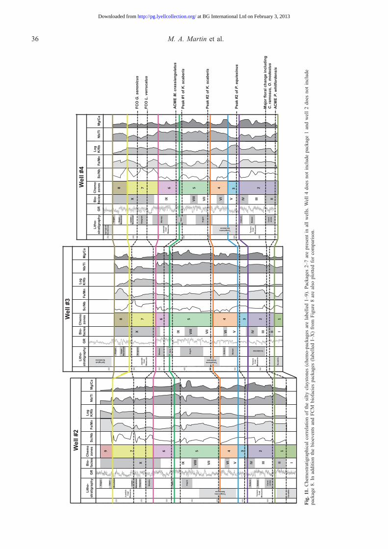
M. A. Martin et al.36
Wel
l #2
200
250
300
350
400
450
500
Wel
l #3
250
300
350
400
450
500
550
Wel
l #4
350
400
450
500
550
600
650
Dura
billa
Juan
dah
Coa
lM
easu
res
Taro
omC
oal
Mea
sure
s
Dura
billa
Kog
an
Uppe
r
Mac
alis
ter
Low
er
Mac
alis
ter
Nang
ram
Wam
bo
Iona
Arg
yle
Aubu
rn
Bulw
er
Con
d-am
ine
SpringbokSandstone
Juan
dah
Coa
lM
easu
res
Taro
omC
oal
Mea
sure
s
Sprin
gbok
Sand
ston
e
Juan
dah
Coa
lM
easu
res
Taro
omC
oal
Mea
sure
s
Kog
an
Uppe
rM
acal
iste
r
Nan
gram
Wam
bo
Arg
yle
Aubu
rn
Bulw
er Condamine
Kog
an
Uppe
rM
acal
iste
r
Low
erM
acal
iste
r
Nan
gram
Wam
bo
Arg
yle
Aubu
rn
Bulw
er
Con
d-am
ine
GR
Fe/M
nN
b/Ti
Sc/N
bM
g/C
aLo
gK
/Rb
Lith
o-
stra
tigra
phy
Bio
-fa
cies I II III
IV
VI
VII
VIII
V
IX
X
II III
IV
V
VI
VII
VIII
IX
X
II III
IV
V
VI
VII
VIII
IX
X
I
GR
Fe/M
nN
b/Ti
Sc/N
bM
g/C
aLo
gK
/Rb
Lith
o-
stra
tigra
phy
Bio
-fa
cies
GR
Fe/M
nN
b/Ti
Sc/N
bM
g/C
aLo
gK
/Rb
Lith
o-
stra
tigra
phy
Bio
-fa
cies
Che
mo
zone
s
Che
mo
zone
sC
hem
ozo
nes
8 7 6 5 4 2 3
TangaloomaSandstone
8 7 6 5 4 2 3 1
9 7 6 5 4 2 3 1
TangaloomaSandstone
TangaloomaSandstone
Iona
Iona
FCO
G. s
enon
icus
FCO
L. v
erru
catu
s
ACM
EM
. cra
ssia
ngul
atus
Maj
or fl
oral
cha
nge
incl
udin
gC
.ram
osus
, O. m
odes
tus
ACM
EP.
whi
tford
ensi
s
Peak
#2
of P
. equ
iexi
nus
Peak
#2
of K
. sca
beris
Peak
#1
of K
. sca
beris
Fig
. 11
. C
hem
ostr
atig
raph
ical
cor
rela
tion
of
the
silt
y cl
ayst
ones
(ch
emo-
pack
ages
are
lab
elle
d 1–
9).
Pac
kage
s 2–
7 ar
e pr
esen
t in
all
wel
ls.
Wel
l 4
does
not
inc
lude
pac
kage
1 a
nd w
ell
2 do
es n
ot i
nclu
de
pack
age
8. I
n ad
diti
on t
he b
ioev
ents
and
FC
M b
iofa
cies
pac
kage
s (l
abel
led
I–X
) fr
om F
igur
e 8
are
also
plo
tted
for
com
pari
son.
at BG International Ltd on February 3, 2013http://pg.lyellcollection.org/Downloaded from
Walloon Subgroup sedimentology and stratigraphy 37
rates of sedimentation and peat preservation, but consistently bracket the Nangram coal. The G. senonicus bioevent is associated with a distinctive peak in the Sc/Nb ratio.
•• Like CM-4, no bioevents are recorded within CM-8 and CM-9.
concluSIonS
Within the studied cored intervals 21 facies and four facies asso-ciations were identified within the WSG. The three sedimentol-ogy wells are too distant (over 80 km apart) for any meaningful facies or lithology correlation. The facies recognized are, how-ever, similar in the three wells and record alluvial plain sedi-mentation throughout the WSG succession.
The pilot studies will need to be expanded to utilize more cored wells and to include the 500+ uncored wells to provide more overlapping datasets between disciplines. This should allow for testing of the limits of new stratigraphical scheme, enhancement of the depositional model and constraint of geo-model inputs. Further core description and sedimentology stud-ies are needed to fine-tune petrophysical calibration; better understand fractures and cleat development in the coals; coal styles, architecture, connectivity and quality trends; gas content distribution; and, hopefully, aid prediction of ‘sweet spots’ and seam connectivity.
Coals in the WSG exhibit two possible ‘end-member’ styles of preservation/development: Class I and II. Their relationship is uncertain but intuitively each class should have a predictable scale, vertical and lateral heterogeneity. ‘Brightening-upward’ and ‘dulling-upward’ trends can be recognized in the coals, the former being the more common. These cycles reflect water table fluctuations and mire expansion/contraction. Further work, including the incorporation of local offset well data, is required to ascertain the stratigraphical and, ultimately, economic signifi-cance of the clastic intervals and ‘brightening-’ and ‘dulling-upward’ trends in the coals.
The integrated stratigraphical approach has provided a new subdivision of the WSG. This will be expanded into neighbouring formations and, more importantly, into a larger area to test the cor-relation of biofacies, bioevents and chemostratigraphical events.
The chemostratigraphy and biostratigraphy wells indicated an overall upwards wetting through Tarooms (see Fig. 3) and then upwards drying through Juandahs. The drying of the climate and development of thicker coal deposits might be coincidence.
There is a broad similarity between the chemostratigraphical zonations of the study wells and their biostratigraphical events, despite some minor discrepancies. The new correlations locally significantly change the depositional system architecture, partic-ularly within the Taroom Coal Measures, and highlight the thickening and thinning of sections between the wells. For cor-relation purposes and geomodelling, the coal seam lithostratigra-phy scheme has been abandoned.
The authors acknowledge QGC for permission to present and publish these results; Paul Wilson and Damien Ryan (QGC) for help with draft-ing some of the figures; and Karen Carr for permission to use her draw-ing ‘Australian Museum Mid Jurassic Plant Community’ (not shown here but used in the Conference presentation). Thanks also go to vari-ous QGC and BG technical staff and to Chris Fielding (University of Nebraska-Lincoln), Carl Watkins (Fugro-Robertson) and Gary Nichols (RHUL) for discussion. Also to Chris Fielding and a further anonymous reviewer for their thorough comments.
rEFErEncES
Andrew, A.S., Whitford, D.J., Hamilton, P.J., Scarano, S. & Buckley, M. 1996. Application of chemostratigraphy to petroleum exploration and field appraisal: An example from the Surat Basin. Society of Petroleum Engineers, no. 37008, 421–429.
Balme, B.E. 1995. Fossil in situ spores and pollen grains: An annotated cata-logue. Review of Palaeobotany and Palynology, 87, 81–323.
Barrón, E., Gómez, J.J., Goy, A. & Pieren, A.P. 2006. The Triassic–Jurassic boundary in Asturias (northern Spain): Palynological char-acterisation and facies. Review of Palaeobotany and Palynology, 138, 187–208.
Binney, H.A., Waller, M.P., Bunting, M.J. & Armitage, R.A. 2005. The inter-pretation of fen carr pollen diagrams: The representation of dryland veg-etation. Review of Palaeobotany and Palynology, 134, 197–218.
Bohacs, K. & Suter, J. 1997. Sequence stratigraphic distribution of coaly rocks: fundamental controls and paralic examples. Bulletin of the American Association of Petroleum Geologists, 81, 1612–1639.
Bradshaw, M.T. & Yeung, M. 1990. The Jurassic palaeogeography of Australia. BMR Record 1990/076. Bureau of Mineral Resources, Geology and Geophysics; Australian Petroleum Industries Research Association, Palaeogeographic Maps Project.
Burger, D. 1994. Palynological studies of the Bundama group and Walloon Coal Measures in the Clarence–Morton Basin. Australian Geological Survey Organization Bulletin, 241, 164–180.
Dettmann, M.E., Molnar, R.E., Douglas, J.G. et al. 1992. Australian Cretaceous terrestrial faunas and floras: Biostratigraphic and biogeo-graphic implication. Cretaceous Research, 13, 207–262.
Diessel, C. 1992. Coal-Bearing depositional systems. Springer-Verlag, Berlin.Diessel, C.F.K. & Gammidge, L. 1998. Isometamorphic variations in the
reflectance and fluorescence of vitrinite – a key to depositional environ-ment. International Journal of Coal Geology, 36, 167–222.
Diessel, C., Boyd, R., Wadsworth, J., Leckie, D. & Chalmers, G. 2000. On balanced and unbalanced accommodation/peat accumulation ratios in the Cretaceous coals from Gates Formation. Western Canada and their sequence stratigraphic significance. International Journal of Coal Geology, 43, 143–186.
Exon, N.F. 1976. Geology of the Surat Basin in Queensland. Bureau of Mineral Resources Bulletin, 166, 1–160.
Exon, N.F. & Burger, D. 1981. Sedimentary cycles in the Surat Basin and global changes of sea level. Bureau of Mineral Resources Journal of Australian Geology and Geophysics, 6, 153–159.
Fielding, C.R. 1993. The Middle Jurassic Walloon coal measures in the type area, The Rosewood–Walloon Coalfield, SE Queensland. Australian Coal Geology, 9, 4–16.
Fielding, C.R., Gray, A.R.G., Harris, G.I. & Salomon, J.A. 1990. The Bowen Basin and overlying Surat Basin. Bureau of Mineral Resources Bulletin, 232, 105–116.
Filatoff, J. 1975. Jurassic palynology of the Perth Basin. Palaeontographica Abteilung B, 154, 1–113.
Fletcher, M.-S. & Thomas, I. 2007. Holocene vegetation and climate change from near Lake Pedder, south-west Tasmania. Journal of Biogeography, 34, 665–677.
Flores, R.M., Keighin, C.W., Ochs, A.M., Warwick, P.D., Bader, L.R. & Murphy, E.C. 1999. Framework Geology of Fort Union Coal in the Williston Basin (Chapter WF). US Geological Survey Professional Paper 1625-A.
Frederiksen, N.O. 1992. Palynology of Mesozoic and lower Tertiary samples from northern, central, and southern Pakistan. US Geological Survey Open-File Report, 92–215.
Gallagher, S.M., Wood, G.R. & Lemon, N.L. 2008. Birkhead Formation chronostratigraphy on the Murteree Horst, South Australia: Identifying and correlating reservoirs and seals. In: PESA Eastern Australasian Basins Symposium III, Sydney, 14–17 September, 169–189.
Gary, A.C., Wakefield, M.I., Johnson, G.W. & Ekart, D.D. 2009. Application of Fuzzy C-Means Clustering to Paleoenvironmental Analysis: Example from the Jurassic, Central North Sea, UK. In: Demchuk, T.D. & Gary, A.C. (eds) Geologic Problem Solving with Microfossils: A Volume in Honor of Garry D. Jones. SEPM Special Publication, 93, 9–20.
Gore, A.J.P. 1983. Mires: Swamp, Bog, Fen and Moor: General Studies. Ecosystems of the World. Elsevier, Amsterdam.
Grant-Mackie, J.A., Aita, Y., Balme, B.E. et al. 2000. Jurassic palaeobio-geography of Australasia. Memoir of the Australasian Association of Palaeontologists, 23, 311–353.
Helby, R., Morgan, R. & Partridge, A.D. 1987. A palynological zonation of the Australian Mesozoic. Memoir of the Association of Australasian Palaeontologists, 4, 1–94.
Hoffmann, K.L., Totterdell, J.M., Dixon, O., Simpson, G.A., Brakel, A.T., Wells, A.T. & McKellar, J.L. 2009. Sequence stratigraphy of Jurassic strata in the lower Surat Basin succession, Queensland. Australian Journal of Earth Sciences, 56, 461–476.
Hubbard, R.N.L.B. & Boulter, M.C. 1997. Mid Mesozoic Floras and Climates. Palaeontology, 40, 43–70.
at BG International Ltd on February 3, 2013http://pg.lyellcollection.org/Downloaded from
M. A. Martin et al.38
Received 14 June 2011; revised typescript accepted 19 June 2012.
Jansson, I.-M. 2006. An Early Jurassic conifer-dominated assemblage of the Clarence-Moreton Basin, eastern Australia. Unpublished MSc thesis, Department of Geology, GeoBiosphere Science Centre, Lund University.
Jarvis, I. & Jarvis, K.E. 1992a. Inductively coupled plasma-atomic emission spectrometry in exploration geochemistry. In: Hall, G.E.M. & Vaughlin, B. (eds) Analytical Methods in Geochemical Exploration. Journal of Geochemical Exploration, Special Issue.
Jarvis, I. & Jarvis, K.E. 1992b. Plasma spectrometry in earth sciences: Techniques, applications and future trends. In: Jarvis, I. & Jarvis, K.E. (eds) Plasma Spectrometry in Earth Sciences. Chemical Geology, 95, 1–33.
Jerrett, R.M., Flint, S.S., Davies, R.C. & Hodgson, D.M. 2011a. Sequence stratigraphic interpretation of a Pennsylvanian (Upper Carboniferous) coal from the central Appalachian Basin, USA. Sedimentology, 58, 1190–1207.
Jerrett, R.M., Davies, R.C., Hodgson, D.M., Flint, S.S. & Chiverrell, R.C. 2011b. The significance of hiatal surfaces in coal seams. Journal of the Geological Society, London, 168, 629–632.
Jones, G.D & Patrick, R.B. 1981. Stratigraphy and coal exploration geology of the northeastern Surat Basin. Geological Society of Australia, Coal Geology Group Journal, 1, 153–163.
Leblang, G.M., Rayment, P.A & Smyth, M. 1981. The Austinvale coal deposit – Wandoan. A palaeoenvironmental analysis. Geological Society of Australia, Coal Geology Group Journal, 1, 185–195.
MacPhail, M.K., Pemberton, M. & Jacobson, G. 1999. Peat mounds of south-west Tasmania: Possible origins. Australian Journal of Earth Sciences, 46, 667–677.
McKellar, J.L. 1996. Palynofloral and megafloral indications of palaeocli-mate in the Late Triassic, Jurassic, and early Cretaceous of southeast-ern Queensland. In: Mesozoic Geology of the Eastern Australia Plate Conference. Geological Society of Australia Inc. Extended Abstracts no. 43, 366–373.
McKellar, J.L. 1998. Late Early to Late Jurassic palynology, biostratigraphy and palaeogeography of the Roma Shelf area, northwestern Surat Basin, Queensland, Australia. PhD thesis, Department of Earth Sciences, The University of Queensland, Vols 1–3 (i-xii + 620 pages of text in Volumes 1–2; 45 plates and 8 app. in Vol. 3).
McKellar, J.L. 2004. Geophysical controls on late Palaeozoic–early Mesozoic geological history and floral succession: Eastern Australia in perspective. Association of Australasian Palaeontologists Memoir, 29, 47–83.
Monteil, E., (coord.) 2006. Australian Mesozoic and Cenozoic Palynology Zonations – updated to the 2004 Geologic Time Scale. Geoscience Australia, Record 2006/23.
Moore, G.T., Hayashida, D.N., Ross, C.A. & Johnson, S.R. 1992. Paleoclimate of the Kimmeridgian/Tithonian (Late Jurassic) world: I. Results using a general circulation model. Palaeogeography, Palaeoclimatology, Palaeoecology, 93, 113–150.
Nielsen, L.H., Petersen, H.I., Dybkjaer, K. & Surlyk, F. 2010. Late-mire deposition, earthquakes and wildfires along a basin margin fault; Ronne Graben, Middle Jurassic, Denmark. Palaeogeography, Palaeoclimatology, Palaeoecology, 292, 103–126.
Partridge, A.D. 2006. Jurassic–Early Cretaceous spore-pollen and dinocyst zonations for Australia. Geoscience Australia Record, 2006/23.
Pearce, T.J., Martin, J.H., Cooper, D. & Wray, D.S. 2010. Chemostratigraphy of the Upper Carboniferous (Pennsylvanian) sequences from the Southern North Sea (United Kingdom). In: Ratcliffe, K.T. & Zaitlin, B.A. (eds) Application of Modern Stratigraphic Techniques: Theory and Case Histories. SEPM Special Publication, 94, 109–127.
Price, P. 1997. Permian to Jurassic palynostratigraphic nomenclature of the Bowen and Surat Basins. In: Green, P.M. (ed.) The Surat and Bowen Basins, south-east Queensland. Queensland Minerals and Energy Review Series, Queensland Department of Mines and Energy, Brisbane, 137–178.
Scott, S., Anderson, B., Crosdale, P., Dingwall, J. & Leblang, G. 2004. Revised Geology and coal seam gas characteristics of the Walloon Subgroup – Surat Basin, Queensland. In: PESA Eastern Australasian Basins Symposium II, 19–22 September, Adelaide, 345–355.
Scott, S., Anderson, B., Crosdale, P., Dingwall, J. & Leblang, G. 2007. Coal petrology and coal seam gas contents of the Walloon Subgroup — Surat Basin, Queensland, Australia. International Journal of Coal Geology, 70, 209–222.
Swarbrick, C.F.J., Gray, A.R.G. & Exon, N.F. 1973. Injune Creek Group – amendments and an addition to the stratigraphic nomenclature in the Surat basin. Queensland Government Mineralogy Journal, 74, 57–63.
Taylor, A.M. & Goldring, R. 1993. Description and analysis of bioturbation and ichnofabric (in Organisms and sediments; relationships and applica-tions). Journal of the Geological Society, London, 150, 141–148.
Turner, S., Bean, L.B., Dettmann, M., McKellar, J.L., McLoughlin, S. & Thulborn, T. 2009. Australian Jurassic sedimentary and fossil succes-sions: Current work and future prospects for marine and non-marine cor-relation. GFF, 131, 49–70.
Veevers, J.J., Powell, C.McA. & Roots, S.R. 1991. Review of seafloor spreading around Australia. 1. Synthesis of the patterns of spreading. Australian Journal of Earth Sciences, 38, 373–389.
Wadsworth, J., Boyd, R., Diessel, C., Leckie, D. & Zaitlin, B.A. 2002. Stratigraphic style of coal and non-marine strata in a tectonically influ-enced intermediate accommodation setting the Mannville Group of the Western Canadian Sedimentary Basin, south-central Alberta. Bulletin of Canadian Petroleum Geology, 50, 507–541.
Wadsworth, J., Boyd, R., Diessel, C. & Leckie, D. 2003. Stratigraphic style of coal and non-marine strata in a high accommodation setting: Falher Member and Gate Formation (Lower Cetaceous), western Canada. Bulletin of Canadian Petroleum Geology, 51, 275–303.
Yago, J.V.R. & Fielding, C.R. 1996. Sedimentology of the Middle Jurassic Walloon Coal Measures in the Great Artesian basin, eastern Australia. Extended Abstracts 43. In: Mesozoic 96, Mesozoic Geology of the Eastern Australia Plate Conference. Geological Society of Australia, Brisbane, 574–575.
Zadeh, L.A. 1965. Fuzzy sets. Information and Control, 8, 338–352.
at BG International Ltd on February 3, 2013http://pg.lyellcollection.org/Downloaded from