Embed Size (px)
Citation preview

Security Issues for Modern Communications Systems: FundamentalElectronic Warfare Tactics for 4G Systems and Beyond
Matthew Jonathan La Pan
Dissertation submitted to the Faculty of theVirginia Polytechnic Institute and State University
in partial fulfillment of the requirements for the degree of
Doctor of Philosophyin
Electrical Engineering
T. Charles Clancy, ChairRobert W. McGwier
Jeff ReedSandeep Shukla
Kathleen Hancock
October 27, 2014Blacksburg, Virginia
Keywords: Communications, Jamming, Cognitive RadioCopyright 2014, Matthew Jonathan La Pan

Security Issues for Modern Communications Systems: FundamentalElectronic Warfare Tactics for 4G Systems and Beyond
Matthew Jonathan La Pan
(ABSTRACT)
In the modern era of wireless communications, radios are becoming increasingly more cog-nitive. As the complexity and robustness of friendly communications increases, so do theabilities of adversarial jammers. The potential uses and threats of these jammers directlypertain to fourth generation (4G) communication standards, as well as future standardsemploying similar physical layer technologies.
This paper investigates a number of threats to the technologies utilized by 4G and futuresystems, as well as potential improvements to the security and robustness of these communi-cations systems. The work undertaken highlights potential attacks at both the physical layerand the multiple access control (MAC) layer along with improvements to the technologieswhich they target.
This work presents a series of intelligent, targeted jamming attacks against the orthogonalfrequency division multiplexing (OFDM) synchronization process to demonstrate some se-curity flaws in existing 4G technology, as well as to highlight some of the potential tools of acognitive electronic warfare attack device. Performance analysis of the OFDM synchroniza-tion process are demonstrated in the presence of the efficient attacks, where in many casescomplete denial of service is induced.
A method for cross ambiguity function (CAF) based OFDM synchronization is presented asa security and mitigation tactic for 4G devices in the context of cognitive warfare scenar-ios. The method is shown to maintain comparable performance to other correlation basedsynchronization estimators while offering the benefit of a disguised preamble. Sync-amblerandomization is also discussed as a combinatory strategy with CAF based OFDM synchro-nization to prevent cognitive jammers for tracking and targeting OFDM synchronization.
Finally, this work presents a method for dynamic spectrum access (DSA) enabled radioidentification based solely on radio frequency (RF) observation. This method represents theframework for which both the cognitive jammer and anti-jam radio would perform cognitivesensing in order to utilize the intelligent physical layer attack and mitigation strategiespreviously discussed. The identification algorithm is shown to be theoretically effective inclassifying and identifying two DSA radios with distinct operating policies.

Contents
List of Figures v
List of Tables x
1 Introduction 1
2 Foundations and Literature Review 5
2.1 Fundamentals of Orthogonal Frequency Division Multiplexing/Multiple Access 5
2.1.1 Orthogonal Frequency Division Multiplexing Synchronization . . . . . 11
2.1.2 Orthogonal Frequency Division Multiplexing Equalization . . . . . . 15
2.2 Dynamic Spectrum Access . . . . . . . . . . . . . . . . . . . . . . . . . . . . 21
2.2.1 Time Frequency Access of the Spectrum . . . . . . . . . . . . . . . . 22
2.2.2 Cognitive Radio . . . . . . . . . . . . . . . . . . . . . . . . . . . . . . 24
2.2.3 Dynamic Spectrum Access Security Challenges . . . . . . . . . . . . . 26
3 Orthogonal Frequency Division Multiplexing Synchronization Attacks 28
3.1 Synchronization Model Analysis . . . . . . . . . . . . . . . . . . . . . . . . . 29
3.1.1 Timing Acquisition Analysis . . . . . . . . . . . . . . . . . . . . . . . 29
3.1.2 Carrier Frequency Offset Estimate Analysis . . . . . . . . . . . . . . 31
3.2 System and Channel Model . . . . . . . . . . . . . . . . . . . . . . . . . . . 38
3.3 Jamming Attacks . . . . . . . . . . . . . . . . . . . . . . . . . . . . . . . . . 40
3.3.1 Timing Acquisition Attacks . . . . . . . . . . . . . . . . . . . . . . . 40
3.3.2 Carrier Frequency Offset Estimation Attacks . . . . . . . . . . . . . . 48
iii
3.4 Simulation and Attack Comparison . . . . . . . . . . . . . . . . . . . . . . . 54
4 Attack Mitigation 62
4.1 Cross Ambiguity Function Based Orthogonal Frequency Division MultiplexingAcquisition . . . . . . . . . . . . . . . . . . . . . . . . . . . . . . . . . . . . 63
4.1.1 Theoretical Analysis of Synchronization with the Ambiguity Function 63
4.1.2 Cross Ambiguity Function Synchronization Performance . . . . . . . 65
4.1.3 Efficient Cross Ambiguity Function Computation . . . . . . . . . . . 68
4.1.4 Computational Complexity . . . . . . . . . . . . . . . . . . . . . . . . 73
4.1.5 Security of Cross Ambiguity Function Based Synchronization . . . . . 77
4.2 Sync-amble Randomization . . . . . . . . . . . . . . . . . . . . . . . . . . . . 78
4.3 Simulation . . . . . . . . . . . . . . . . . . . . . . . . . . . . . . . . . . . . . 80
5 Adaptive Dynamic Spectrum Access Radio Warfare 85
5.1 Hierarchical Dynamic Spectrum Access Networks . . . . . . . . . . . . . . . 87
5.2 Traffic Modeling . . . . . . . . . . . . . . . . . . . . . . . . . . . . . . . . . . 89
5.3 System Description . . . . . . . . . . . . . . . . . . . . . . . . . . . . . . . . 89
5.3.1 Classification with Self Organizing Maps . . . . . . . . . . . . . . . . 90
5.3.2 Probabilistic Radio Representation Using Hidden Markov Models . . 93
5.3.3 Classifying Unknown Radios . . . . . . . . . . . . . . . . . . . . . . . 94
5.4 Simulation and Analysis . . . . . . . . . . . . . . . . . . . . . . . . . . . . . 95
6 Conclusion and Future Work 98
7 Bibliography 101
iv

List of Figures
1.1 Illustration of spectrum allocation in the United States from 2003. This dia-gram of the radio spectrum frequency allocations in the United States illus-trates the problem of spectral crowding at as the demand for wireless appli-cations increases. . . . . . . . . . . . . . . . . . . . . . . . . . . . . . . . . . 2
1.2 Open Systems Interconnection (OSI) network architecture model for commu-nications systems. The fundamental level encompasses the digital modulationstructure of a system, which is OFDM for the wireless systems analyzed inthis work. The data link layer is an abstraction of processes like multiple useraccess (MAC) and is sometimes referred to as the MAC layer. The conceptof DSA for wireless systems refers to this second layer. . . . . . . . . . . . . 3
2.1 Frequency division multiplexing. . . . . . . . . . . . . . . . . . . . . . . . . . 6
2.2 Synthesis of OFDM symbols and their fundamental representation in both thetime and frequency domain [1]. . . . . . . . . . . . . . . . . . . . . . . . . . 8
2.3 OFDM transmitter. . . . . . . . . . . . . . . . . . . . . . . . . . . . . . . . . 10
2.4 OFDM receiver. . . . . . . . . . . . . . . . . . . . . . . . . . . . . . . . . . . 10
2.5 The timing metric M(d) for an OFDM preamble symbol in a window of 3symbols length . . . . . . . . . . . . . . . . . . . . . . . . . . . . . . . . . . 13
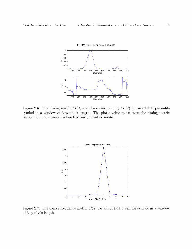
2.6 The timing metric M(d) and the corresponding ∠P (d) for an OFDM preamblesymbol in a window of 3 symbols length. The phase value taken from thetiming metric plateau will determine the fine frequency offset estimate. . . . 14
2.7 The coarse frequency metric B(g) for an OFDM preamble symbol in a windowof 3 symbols length . . . . . . . . . . . . . . . . . . . . . . . . . . . . . . . . 14
2.8 A hypothetical wireless channel environment, with examples of possible inter-ference effects to a wireless signal. . . . . . . . . . . . . . . . . . . . . . . . . 16
v

2.9 The continuous time magnitude response of a multipath channel. Each deltafunction is weighted with a complex coefficient corresponding to a specificsignal path. . . . . . . . . . . . . . . . . . . . . . . . . . . . . . . . . . . . . 17
2.10 The use of pilot tones for OFDM equalization. The orange subcarriers areused to transmit data to the receiver, while the green subcarriers representthe pilots used at the receiver to take partial channel measurements for equal-ization. The symbols transmitted over the pilots are generally known at thereceiver in order to construct a reliable channel estimate. . . . . . . . . . . 19
2.11 A frequency selective fading channel due to multipath interference. The di-agrams on the left show the magnitude response of a transmitted signal andthe frequency selective fading channel. The diagram on the right shows themagnitude response of the received signal after passing through the frequencyselective channel. The coherence bandwidth, Bc, is shown on radio channeldiagram. . . . . . . . . . . . . . . . . . . . . . . . . . . . . . . . . . . . . . 20
2.12 Visual comparison of three multiple access schemes. TDMA and FDMA di-vide user resources in time and frequency, respectively. CDMA uses orthog-onal codes that allow multiple users to share concurrent time and frequencyresources without interfering with one another [2]. . . . . . . . . . . . . . . 23
2.13 Example listing of available spectrum resources due to television band whitespace according to Spectrum Bridge’s Show My White Space tool. The liston the right shows where television band devices could be used by televisionband devices (TVBDs). . . . . . . . . . . . . . . . . . . . . . . . . . . . . . 24
2.14 Cognitive radio decision flow architecture. A cognitive radio is constantlygoing through this loop in order to make decisions in and learn from its RFenvironment. Cognitive radios have the ability to sense their surroundingspectrum and make decisions, but they also theoretically have the ability tolearn and update their strategies and policies. . . . . . . . . . . . . . . . . . 25
2.15 High level examples of DSA radio jammers. The blue bars represent DSAuser energy and the red represents the malicious device. Four attacks areshown that target the DSA radios sensing capability. The barrage jammeroccupies a single channel so that the DSA radio perceives it as unavailable,the herding jammer guides the DSA radio to a chosen channel, the followerjammer frequency hops with the DSA radio and the sweeping jammer movesincrementally across the channels in a given band. . . . . . . . . . . . . . . 26
3.1 Lower bound on the peak value of the timing metric plateau relative to SNR 31
3.2 Lower bound on the coarse frequency offset estimator peak at the correctfrequency offset relative to the effective SNR after channel fading. . . . . . . 36
vi

3.3 The physical jamming scenario . . . . . . . . . . . . . . . . . . . . . . . . . . 38
3.4 Timing estimate error as a function of the effective SNR at the receiver. . . . 42
3.5 Computed autocorrelation of half of the first preamble symbol minus the cyclicprefix. . . . . . . . . . . . . . . . . . . . . . . . . . . . . . . . . . . . . . . . 46
3.6 Degradation as a function of the relative frequency offset of received OFDMsymbols using various subcarrier modulations . . . . . . . . . . . . . . . . . 49
3.7 Estimate of the angle of P (d) at the receiver based on the SJR of the phasewarping attack with randomly generated frequency offsets. The estimate con-verges to the fractional frequency offset of the transmitter at high SJRs andthe jammer at low SJRs. . . . . . . . . . . . . . . . . . . . . . . . . . . . . . 51
3.8 Symbol timing error rate as a function of the SJR of the false preamble timingattack. . . . . . . . . . . . . . . . . . . . . . . . . . . . . . . . . . . . . . . . 55
3.9 Symbol timing error rate as a function of the SJR at the receiver caused bythe preamble warping attack at an SNR of 20 dB. . . . . . . . . . . . . . . . 56
3.10 Timing estimate error rate as a function of SJR for the preamble nulling attackat an SNR of 20 dB. . . . . . . . . . . . . . . . . . . . . . . . . . . . . . . . 57
3.11 Frequency offset estimation error rate as a function of the SJR of three phasewarping attacks with varying levels of situational knowledge. . . . . . . . . . 58
3.12 Frequency offset estimation RMS error as a function of the SJR of the phasewarping attack with channel knowledge. . . . . . . . . . . . . . . . . . . . . 58
3.13 Frequency offset estimation error rate as a function of the SJR of the differ-ential scrambling attack with channel knowledge. . . . . . . . . . . . . . . . 60
3.14 Frequency offset estimation RMS error as a function of the SJR of the differ-ential scrambling attack with channel knowledge. . . . . . . . . . . . . . . . 61
4.1 CAF surface used to perform timing and frequency offset estimation for OFDMsynchronization. The location of the distinct peak in the CAF produces thevalues of the symbol timing point and the carrier frequency offset estimateused for synchronization at the receiver. . . . . . . . . . . . . . . . . . . . . 64
4.2 Theoretical snap shot of a normalized CAF plane at the frequency offset N ffs
.The timing correlation peaks correspond to the magnitude and the locationof the theoretical FIR filter taps of the multipath channel. As long as thestrongest peak occurs within the range of the cyclic prefix–denoted by the redbox–then the receiver will be able to estimate a valid timing point. If thestrongest path falls after the cyclic prefix–marked by the gray area–then thetiming point will be invalid. . . . . . . . . . . . . . . . . . . . . . . . . . . . 67
vii
4.3 Lower bound on the normalized cross ambiguity function peak term relativeto SNR. Results are shown over multiple values of |hi| in order to illustratehow multipath fading can impact the synchronization process. . . . . . . . . 68
4.4 The coarse timing CAF method of determining the timing point and thecarrier frequency offset for an OFDM system. Each of these values are subse-quently outputted to timing and frequency correction blocks. . . . . . . . . . 71
4.5 The coarse frequency CAF method of determining the timing point and thecarrier frequency offset for an OFDM system. Each of these values are subse-quently outputted to timing and frequency correction blocks. . . . . . . . . . 73
4.6 Comparison of the computational complexity between the coarse time CAFcomputation method and the coarse frequency computation method. Thecomparison is shown across a range of power of 2 subcarrier values and fordiffering values of the timing point search range —D—. . . . . . . . . . . . 76
4.7 Example of Sync Signals within Frames . . . . . . . . . . . . . . . . . . . . . 78
4.8 Time-Frequency diagram of an 4G frame using OFDM. . . . . . . . . . . . . 79
4.9 Symbol timing and carrier frequency offset estimation performance of thecoarse frequency domain method. The plot shows the percentage of incorrectcomputed values, where errors are considered to be timing points outside of thecyclic prefix range and frequency offset estimates more than five hundredthsof a subcarrier away from the actual frequency offset. . . . . . . . . . . . . 81
4.10 Symbol timing and carrier frequency offset estimation performance of thecoarse time domain method. The plot shows the percentage of incorrect com-puted values, where errors are considered to be timing points outside of thecyclic prefix range and frequency offset estimates more than five hundredthsof a subcarrier away from the actual frequency offset. . . . . . . . . . . . . . 82
4.11 Performance of the carrier frequency offset estimation for both the coarse timeand coarse frequency CAF computation methods vs. the Cramer-Rao lowerbound. The measured values represent the root mean squared error values ofthe frequency offset estimates. . . . . . . . . . . . . . . . . . . . . . . . . . . 82
4.12 Comparison of performance between Schmidl and Cox’s method and the CAFbased synchronization algorithm in the presence of the phase warping attack 83
4.13 Timing estimate error rate as a function of SJR for the CAF synchronizationalgorithm vs. the Schmidl and Cox synchronization algorithm in the presenceof various attacks. The CAF synchronization mitigates the power efficientattacks at the expense of acquisition complexity. . . . . . . . . . . . . . . . 84
viii

5.1 Time-frequency diagram illustrating ’holes’ in the wireless spectrum due toinactivity. . . . . . . . . . . . . . . . . . . . . . . . . . . . . . . . . . . . . . 86
5.2 Generalized decision engine architecture for a secondary DSA radio. The radioevaluates the RF environment after each transition to determine the next one.The green and orange arrows show the single difference between the two radiomodes’ behaviors. The state transition behavior depends only on the currentstate. . . . . . . . . . . . . . . . . . . . . . . . . . . . . . . . . . . . . . . . . 87
5.3 A visualization of the spectrum sensing information that secondary DSA ra-dios use in their decision engine. Channel power measurements, in blue, aretaken within the bandwidth of interest and compared to the decision thresholds. 88
5.4 The high level architecture for the proposed system. The green arrows showthe signal flow for both the training and identification phases of the system.Each different class of radio trains against this system in order for an unknowntransmitter to be identified within a known class of radios. . . . . . . . . . 89
5.5 Neighbor distance maps for the self organizing maps constructed from theRF observations from each radio mode. These maps are an interpretation ofthe unified distance matrix that represents the topology of the self organizingmap. Black represents the greatest distances between neurons and yellowrepresents the least distance. . . . . . . . . . . . . . . . . . . . . . . . . . . 92
5.6 Sample assignments for each RF observation training vector to the self orga-nizing map. These plots represent the discretization of the observation spacevia assigning observation samples to different neurons in the map. The sizeof the blue hexagon in each neuron represents the frequency of an observationbeing assigned to it. . . . . . . . . . . . . . . . . . . . . . . . . . . . . . . . 92
ix

List of Tables
3.1 Situational knowledge provided to each jammer for simulation . . . . . . . . 55
5.1 Radio Identification Success Rates Using O1, 1 Map . . . . . . . . . . . . . . 95
5.2 Radio Identification Success Rates Using O1, 2 Maps . . . . . . . . . . . . . 96
5.3 Radio Identification Success Rates Using O2, 1 Map . . . . . . . . . . . . . . 96
5.4 Radio Identification Success Rates Using O2, 2 Maps . . . . . . . . . . . . . 97
x

Chapter 1
Introduction
Wireless communication systems are prevalent across a range of platforms. Their applica-tions are continuing to increase with time, often times substituting for wired communicationssystems due to their inherent benefits. The increasing need for wireless technology presentsa distinct set of challenges and requirements based upon the available resources.
The availability of wireless communication resources is a good starting point for understand-ing the issue. There are a variety of resources which are important and essential to anycommunications system, however, in the context of modern wireless communications the onethat always seems to pop up in conversation is spectrum. Spectrum refers to the availablebandwidth appropriated for wireless communications applications along the usable radio fre-quency spectrum. In order for any wireless communication system to operate, it must havesome spectrum to operate on. But in todays society the demand for spectrum is startingto exceed the supply, which has led to spectral crowding. Figure 1.1 depicts the limitedavailability of spectrum in the United States.
At the same time that spectral limitations have started to become a concern, wireless appli-cations that require an increasing amount of capacity and throughput continue to develop.This problem is perhaps most visible in the realm of cellular communications, where theemergence of smart phones, tablets and similar devices have brought forth an overwhelmingdemand for high data rates. In order to meet the demands of cellular networks, there are anumber of emerging technologies which have been developed to maximize spectral efficiency.In particular, there is the set of fourth generation (4G) wireless standards which are shapingthe way that available communications resources are utilized.
The strategies for improving efficiency in wireless communication both offered by 4G sys-tems and that are being developed for future systems are numerous. The research in thispaper is centered around some of the most important technological developments made atthe fundamental layers of the Open Systems Interconnection (OSI) network architecturestack. Figure 1.2 illustrates an example of how this stack loosely defines the layers of a
1

Matthew Jonathan La Pan Chapter 1. Introduction 2
Figure 1.1: Illustration of spectrum allocation in the United States from 2003. This diagramof the radio spectrum frequency allocations in the United States illustrates the problem ofspectral crowding at as the demand for wireless applications increases.

Matthew Jonathan La Pan Chapter 1. Introduction 3
Figure 1.2: Open Systems Interconnection (OSI) network architecture model for communi-cations systems. The fundamental level encompasses the digital modulation structure of asystem, which is OFDM for the wireless systems analyzed in this work. The data link layeris an abstraction of processes like multiple user access (MAC) and is sometimes referred toas the MAC layer. The concept of DSA for wireless systems refers to this second layer.
communications system from user to user. Specifically, we will analyze the use of orthogonalfrequency division multiplexing and multiple access (OFDM/A) in current implementations,as well as dynamic spectrum access (DSA) technology and for future implementations ofwireless systems. OFDM, which is already a part of 4G standards [3, 4], offers a wealth ofadvantages to 4G systems at the physical layer. DSA is at the forefront of future communi-cations technology, and will most likely be incorporated in either later 4G or 5G standardsat the MAC layer.
While the feasibility of OFDM and DSA for modern systems offers significant advantages tousers, many of the techniques for implementing these technologies have been developed forcommercial systems where capacity and throughput demand is placed at a higher premiumthan security concerns. The emergence of electronic warfare for wireless communication sys-tems has put a square focus on security issues for 4G systems. The emergence of OFDMand DSA for 4G systems gives rise to a wealth of problems on both the offensive and defen-sive side of electronic warfare tactics. This research is focused on a particular set of thoseproblems, with emphasis on incorporating electronic warfare considerations in to systemimplementations.
The novel contributions of this work are as follows:

Matthew Jonathan La Pan Chapter 1. Introduction 4
• A suite of power efficient jamming attacks that target OFDM synchronization at boththe timing acquisition and carrier frequency offset estimation processes.
• An efficient cross ambiguity function based OFDM synchronization approach.
• A dynamic spectrum access radio classification and identification approach using stochas-tic modeling and machine learning algorithms.
These items, as well as the accompanying mathematical analysis, are the original work ofthe author, and it should be pointed out that the use of we in this paper is in general refer-ence to the audience. In addition, the remainder of this work will be organized as follows.Chapter 2 presents the theoretical foundations and relevant literature to the presented re-search. Chapter 3 analyzes the performance of OFDM synchronization security and presentsa number of possible security threats in the form of efficient jamming attacks. Chapter 4discusses OFDM attack mitigation and security strategies, including synchronization withthe cross ambiguity function and frame level ’sync-amble’ randomization. Chapter 5 coversan algorithm for dynamic spectrum access radio identification. Finally, Chapter 6 containsthe conclusions of this work as well as proposed future work.

Chapter 2
Foundations and Literature Review
Orthogonal frequency division multiplexing (OFDM) is a multicarrier digital modulationscheme. As suggested by its name, OFDM utilizes an orthogonal basis for performing fre-quency division multiplexing. There are multiple motivations for this technique, perhapsthe most basic being the avoidance of intersymbol interference (ISI). ISI occurs when one ormore symbols in a wireless communication system interferes with another symbol. ISI canbe a catastrophic detriment to any communication symbol if it is not mitigated. OFDM usesthe discrete Fourier transform (DFT) as an orthogonal basis. This approach also ensuresspectral efficiency because OFDM does not require guard bands between subcarriers, as op-posed to traditional FDM where they needed to protect against co-channel interference. Inaddition, the structure of OFDM allows for lower complexity equalization in the frequencydomain. This is an important feature of OFDM that ties in to mitigating ISI that is causedby multipath interference.
Based on the evolving landscape in the world of wireless communications, OFDM is be-coming a popular choice for physical layer modulation. In order to grasp this migration,it is essential to understand the fundamentals, advantages and disadvantages of OFDM forwireless communications. Since a portion of the basis for choosing OFDM as a physical layermodulation scheme is rooted in its compatibility with DSA schemes, it makes sense to coverthe foundation of both technologies.
2.1 Fundamentals of Orthogonal Frequency Division
Multiplexing/Multiple Access
Frequency division multiplexing (FDM) is the basis for the development of OFDM tech-nology. FDM is predicated on the transmission of multiple streams of data over the samemedium via frequency domain separation. For digital modulation schemes, baseband signals
5

Matthew Jonathan La Pan Chapter 2. Foundations and Literature Review 6
0
0
0 B3/2 -B3/2
B2/2 -B2/2
B1/2 -B1/2
f1 f1+B1/2 f1-B1/2 f2 f2+B2/2 f2-B2/2 f3 f3+B3/2 f3-B3/2
Channel 1 Channel 2 Channel 3
Figure 2.1: Frequency division multiplexing.
are modulated to carrier frequencies via
pk =K−1∑
k=0
Re(bk(t)) cos(2πfkt) + Im bk(t) sin(2πfkt) (2.1)
and transmitted simultaneously according to
s =K−1∑
k=0
pk(t). (2.2)
In order for these signals to be recoverable, they must be separable in the frequency domain.This means that each separate passband signal pk with bandwidth Bk must satisfy
fk +Bk
2≤ fk+1 −
Bk+1
2. (2.3)
In practical scenarios, however, the signals pk will have some amount of energy outside oftheir bandwidths Bk. Extra frequency domain spacing, often referred to as guard bands, areused in order to ensure minimal interference between adjacent channels.An example of thistechnique is shown in Figure 2.1.
While this technique is effective for the transmission of multiple signals over a single medium,the frequency spacing and the use of the guard bands make it somewhat spectrally inefficient,
Matthew Jonathan La Pan Chapter 2. Foundations and Literature Review 7
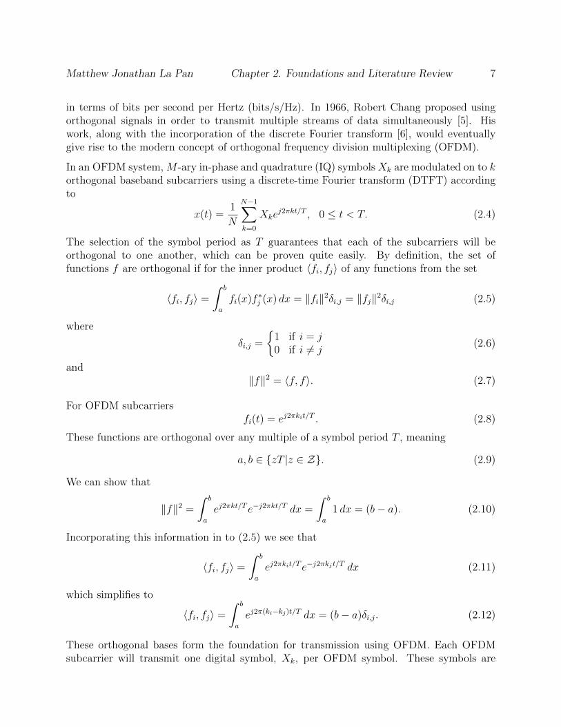
in terms of bits per second per Hertz (bits/s/Hz). In 1966, Robert Chang proposed usingorthogonal signals in order to transmit multiple streams of data simultaneously [5]. Hiswork, along with the incorporation of the discrete Fourier transform [6], would eventuallygive rise to the modern concept of orthogonal frequency division multiplexing (OFDM).
In an OFDM system, M -ary in-phase and quadrature (IQ) symbols Xk are modulated on to korthogonal baseband subcarriers using a discrete-time Fourier transform (DTFT) accordingto
x(t) =1
N
N−1∑
k=0
Xkej2πkt/T , 0 ≤ t < T. (2.4)
The selection of the symbol period as T guarantees that each of the subcarriers will beorthogonal to one another, which can be proven quite easily. By definition, the set offunctions f are orthogonal if for the inner product 〈fi, fj〉 of any functions from the set
〈fi, fj〉 =
∫ b
a
fi(x)f ∗j (x) dx = ‖fi‖2δi,j = ‖fj‖2δi,j (2.5)
where
δi,j =
{1 if i = j0 if i 6= j
(2.6)
and‖f‖2 = 〈f, f〉. (2.7)
For OFDM subcarriersfi(t) = ej2πkit/T . (2.8)
These functions are orthogonal over any multiple of a symbol period T , meaning
a, b ∈ {zT |z ∈ Z}. (2.9)
We can show that
‖f‖2 =
∫ b
a
ej2πkt/T e−j2πkt/T dx =
∫ b
a
1 dx = (b− a). (2.10)
Incorporating this information in to (2.5) we see that
〈fi, fj〉 =
∫ b
a
ej2πkit/T e−j2πkjt/T dx (2.11)
which simplifies to
〈fi, fj〉 =
∫ b
a
ej2π(ki−kj)t/T dx = (b− a)δi,j. (2.12)
These orthogonal bases form the foundation for transmission using OFDM. Each OFDMsubcarrier will transmit one digital symbol, Xk, per OFDM symbol. These symbols are

Matthew Jonathan La Pan Chapter 2. Foundations and Literature Review 8
OFDM symbol windowing - allows other OFDM symbols transmission
0 0.5 1 1.5 2 2.5 3−2
−1
0
1
2
3
4Time domain OFDM signal for 5 subcarriers modulated with {1,1,1,1,1}.
0 0.5 1 1.5 2 2.5 3−2
−1
0
1
2
3
4Time domain rectangular windowed OFDM signal
time / ( NT)
(a) Time domain before/after windowing.
−6 −4 −2 0 2 4 60
0.2
0.4
0.6
0.8
1Frequency domain OFDM signal for 5 subcarriers modulated with {1,1,1,1,1}.
subcarrier k
Spec
trum
−6 −4 −2 0 2 4 6−0.5
0
0.5
1
1.5Frequency domain rectangular windowed OFDM signal
subcarrier k
Spec
trum
(b) Freq. domain before/after windowing.
• before windowing: X(f ) = X(k)±(f ° kfo)
• after windowing:X(f )W (f ) = X(k)±(f ° kfo) ≠ sinc(f/fo) = X(k)sinc(f/fo ° k)
Note: X(f) from here on will be assumed to be windowed with rectangular window.
CENTRE FORWIRELESS
COMMUNICATIONS
6 Ho Chin Keong: Overview on OFDM Design
Figure 2.2: Synthesis of OFDM symbols and their fundamental representation in both thetime and frequency domain [1].
typically chosen from an M -ary digital symbol mapping used to modulate binary data.OFDM is able to transmit using phase-shift keying (PSK) and amplitude shift keying (ASK),as well as quadrature amplitude modulation (QAM), which is a combination of the two.
While the relationship in equation 2.4 is useful for analyzing subcarrier orthogonality, OFDMsymbols are actually generated discretely according to the DFT
x[n] =1
N
N−1∑
k=0
Xkej2πkn/N , n = 0, 1, ..., N − 2, N − 1. (2.13)
The sequence x[n] represents a single OFDM symbol over a the symbol period T , where
N = fsT (2.14)
where fs is the sampling frequency in Hz for a given system. In an OFDM system, Nrepresents both the number of samples per symbol and the number of subcarriers.
The baseband signal x[n] is sent to a digital-to-analog converter (DAC) then either to thereceiver either at baseband, or to RF an modulation stage, the latter being the case forwireless systems. The receiver recovers the modulated symbols Xk using the conjugatetransform
Xk =N−1∑
k=0
x[n]e−j2πkn/N , n = 0, 1, ..., N − 2, N − 1. (2.15)
The resulting IQ symbols are then estimated, processed and demodulated at the receiver,where the underlying information bits can ultimately be decoded.
As shown in Figure 2.2, OFDM is a highly spectrally efficient modulation scheme. It hasbeen shown that OFDM is up to twice as spectrally efficient as single carrier modulation [7].

Matthew Jonathan La Pan Chapter 2. Foundations and Literature Review 9
The spectral efficiency, η, of OFDM is given by the equation
η =NRs
(N + 1)fo(2.16)
where Rs is the symbol rate and fo represents the bandwidth of a single subcarrier. Fromthis equation we see that as N →∞, η → R
fo. Alternatively, the spectral efficiency of single
carrier modulation schemes is given by
η =Rs
2fo. (2.17)
It should be noted that single carrier modulations can be windowed in order to somewhatimprove spectral efficiency, while OFDM subcarriers can not be windowed due to the orthog-onality requirement. However, the efficiency gain from windowing is much less significantthan the factor of 2.
Increase in spectral efficiency is a major motivation for the movement of modern systemstoward utilizing OFDM technology at the physical layer, however, it is not the only reason.As described in equation (2.13), OFDM symbols are typically generated using a DFT. Thisis a major advantage for OFDM on two fronts. The first is that there are a large numberof efficient algorithms for computing the DFT. The algorithms within this family are oftenreferred to communally as the fast Fourier transform (FFT). While explicit computation ofan N point DFT requires O(N2) computations, existing efficient algorithms like the radix-2 Cooley-Tukey algorithm can compute the FFT of a complex sequence in O(N log(N))computations. The second advantage–which is really an extension of the first–is that thereis a wide range of low cost signal processing hardware designed specifically to compute theFFT, making OFDM modulators and demodulators relatively inexpensive. And, as we willdiscuss in subsequent sections, the FFT based structure of OFDM will allow for portionsof the modulation control processes of synchronization and equalization to be performedefficiently in the frequency domain.
The choice of an orthogonal basis for OFDM means that there is zero inter-symbol inter-ference (ISI) and zero inter-carrier interference (ICI) in an ideal communication setting. Inorder to modulate baseband symbols with the FTT, an OFDM transmitter first takes a serialstream of digital samples and parallelizes them. The symbols are then converted to base-band digital symbols, also called IQ symbols. The specific digital modulation used on thesubcarriers depends on the transmitter, and can be varied from low order modulations–suchas binary phase-shift keying–to modulations with much higher bits per symbol like 256 bitquadrature amplitude modulation (256 QAM). The symbols are then modulated on to theindividual subcarriers by assigning each one to a frequency bin and performing an inverseFFT (IFFT). Intuitively, the signal is being ’constructed’ in the frequency domain and thenthe time domain signal is generated via IFFT. The real and imaginary parts of the signalare then split and can be transmitted on the carrier frequency using IQ modulation. TheOFDM receiver is simply the inversion of this process. The basic block diagrams of theOFDM transmitter and receiver are shown in Figures 2.3 and 2.4.

Matthew Jonathan La Pan Chapter 2. Foundations and Literature Review 10
Figure 2.3: OFDM transmitter.
Figure 2.4: OFDM receiver.

Matthew Jonathan La Pan Chapter 2. Foundations and Literature Review 11
While these simplified models of an OFDM transmitter and receiver covers the basic functionsof modulation and demodulation, there are important processing blocks required for coherentOFDM communication which are omitted. In order for an OFDM transmitter and receiver tocommunicate in dynamic, wireless environments, it is necessary to facilitate synchronizationbetween the two, and equalization at the receiver due to multipath channel effects. Theseprocesses, detailed in the next couple of sections, add complexity at both the transmitter andreceiver. The transmitter is generally tasked with injecting control symbols in to outgoingdata streams in order to enable synchronization and equalization at the receiver. The receiveris tasked with processing these overhead symbols in order to mitigate timing and frequencyoffsets that result in loss of subcarrier orthogonality and subsequent ICI, as well as multipatheffects that can lead to ISI at the receiver. While idealized OFDM transmitter and receivermodels are useful for explaining the underlying theory and motivation for using OFDM,communication with OFDM in most realistic wireless settings requires these added processes.
2.1.1 Orthogonal Frequency Division Multiplexing Synchroniza-tion
All practical wireless communications systems are susceptible to timing and frequency errorsbetween the transmitter and the receiver. This is due to clock differences between thetwo ends and the uncertainty of symbol start times in burst communications. For thisreason, synchronization between the terminals is required for certain communication systems,depending on their design.
Assuming that the synchronization symbol sent resembles an ordinary data symbol, and thatthe channel from the transmitter to the receiver can be modeled as an AWGN multipathchannel with finite length impulse response, the sampled signal at the receiver after basebandconversion is represented as
rn =
(C−1∑
k=0
xn−d−khk
)e2πj
ffsn + nn (2.18)
where the subscript n represents the sample index and spans the search area for the trainingsymbol, d is the delay value and timing point of the symbol, C is the length of the channelapproximation, f represents the carrier frequency offset and n is the noise term.
Synchronization is both critical and prerequisite to successful communication using OFDM.Without properly accounting for timing and carrier frequency offset at the receiver, OFDMsystem performance will be massively degraded [7, 8]. The resulting inter-symbol inter-ference (ISI) and inter-carrier interference (ICI) in many cases can prevent communicationaltogether.
There are various methods for performing OFDM synchronization [9, 10, 11, 12, 13]. How-ever, one method that is very frequently employed for OFDM systems is presented in [14].

Matthew Jonathan La Pan Chapter 2. Foundations and Literature Review 12
This method is employed in 802.11 standards, as well as WiMAX. The synchronizationmethod presented by Schmidl and Cox provides a high level of performance–the methodprovides the maximum likelihood (ML) estimate for the OFDM synchronization symbol in-cluding channel effects–and is therefore the method analyzed for comparative analysis in thispaper. It is important to note, that while this method is not used in every OFDM system, itis one of the most practical high performance algorithms available for synchronization, mak-ing it a great point of reference for performing mathematical analysis on the synchronizationprocess.
The synchronization method proposed in [14] has three main stages–symbol timing estima-tion, fine carrier frequency offset estimation and correction, and coarse carrier frequencyoffset estimation. These stages are performed sequentially in the order listed. This algo-rithm is based on the use of specific preamble symbols, transmitted at the beginning of everyframe. Because of the particular structure of this synchronization algorithm, the preamblesymbols have a very specific structure as indicated in [14].
The first step in the synchronization process is the estimation of symbol timing. Only the firstpreamble symbol is used for the timing stage. Once the complex time domain samples areobtained after radio frequency (RF) down conversion then the timing estimation algorithmis carried out. A sliding window of L samples is used to search from the preamble, where Lis equal to the length of half of the first preamble symbol excluding the cyclic prefix. Twoterms are computed for timing estimation. The first according to
P (d) =L−1∑
m=0
(r∗d+mrd+m+L) (2.19)
and the second according to
R(d) =L−1∑
m=0
|rd+m+L|2 (2.20)
where d is the time index which corresponds to the first sample taken in the window and r isthe length-L vector of received symbols. The ( )∗ notation represents complex conjugation.These two terms are used to compute the timing metric M(d) according to
M(d) =|P (d)|2R(d)2
(2.21)
which determines the symbol timing.
This metric will generate a plateaued peak where the maximum values begin at d = d, withthe point d being at the beginning of the preamble, and end when d = d + (Tcp − Tch)fs,where Tcp is the period of the cyclic prefix and Tch is the length of the channel impulseresponse, corresponding to its delay spread. The symbol timing estimate can be taken fromanywhere on the plateau, which will be the length of the cyclic prefix minus the length ofthe channel impulse response. This timing estimate will tell the receiver the starting point

Matthew Jonathan La Pan Chapter 2. Foundations and Literature Review 13
−500 −400 −300 −200 −100 0 100 200 300 400 500
0.1
0.2
0.3
0.4
0.5
0.6
0.7
0.8
0.9
OFDM Preamble Timing Metric
Tim
ing
Me
tric
Symbol Timing (samples)
Figure 2.5: The timing metric M(d) for an OFDM preamble symbol in a window of 3 symbolslength
of the window of samples to grab in order to process an incoming frame. Once this stageis performed, the receiver will take the samples from the timing point and correct for thecarrier frequency error between the transmitter and the receiver.
Carrier frequency offset estimation is the final step of the synchronization process. This stagecorrects for the error introduced by the clocks at both the transmitter and the receiver. Thereare actually two sub-stages within frequency correction. The first is fine frequency correctionand the second is coarse frequency correction. The fine frequency correction ∆f is estimatedusing
∆f = ∠(P (d))/πT (2.22)
where T is the period of a single preamble symbol without its cyclic prefix and d is takenfrom anywhere along the timing metric plateau.
The coarse frequency error estimation is the final step in the synchronization process, andfinally employs the use of the second preamble symbol and the differentially modulated PNsequence. First, FFTs–the length of the symbol period without the cyclic prefix–of each ofthe symbols are taken. A coarse frequency metric is then computed in order to determinethe number of bins that the symbols are shifted in either direction according to
B(g) =
∣∣∑k∈X R
∗1,k+2gv
∗kR2,k+2g
∣∣2
2(∑
k∈X |R2,k|2)2(2.23)
where R1,k+2g and R2,k+2g represent the DFT of rd+m and rd+m+L, respectively. These termsare later defined explicitly in equation (3.20). The term g represents the circular shift ofthe frequency bins of each of the DFT terms. For this equation, the set X represents all of
Matthew Jonathan La Pan Chapter 2. Foundations and Literature Review 14
100 200 300 400 500 600 700 800 900 1000
−2
0
2
d (samples)
6P(d)
OFDM Fine Frequency Estimate
100 200 300 400 500 600 700 800 900 1000
0.2
0.4
0.6
0.8
1
d (samples)
M(d)
Figure 2.6: The timing metric M(d) and the corresponding ∠P (d) for an OFDM preamblesymbol in a window of 3 symbols length. The phase value taken from the timing metricplateau will determine the fine frequency offset estimate.
Figure 2.7: The coarse frequency metric B(g) for an OFDM preamble symbol in a windowof 3 symbols length

Matthew Jonathan La Pan Chapter 2. Foundations and Literature Review 15
the subcarrier bins which are occupied by both preamble symbols (either even or odd). Thedifferential PN sequence shows up as
vk =√
2X2,k
X1,k
. (2.24)
where the terms X1,k and X2,k represent the length L DFT of the first and second preamblesymbols. It is important to note that
Xi,k =2L−1∑
n=0
xn+N(i−1)e−2πjkn/2L. (2.25)
The overall frequency offset is
∆f = ∠(P (d))/πT + 2gmax/T (2.26)
where gmax is the value of g that maximizes B(g) in equation (2.23), specifically gmax = f2.
Once the overall frequency offset between the transmitter and the receiver has been deter-mined, the signal acquisition process is complete and information symbols can be transmit-ted.
2.1.2 Orthogonal Frequency Division Multiplexing Equalization
Wireless channels present a number of distinct challenges for communications systems. Thereare a number of channel effects that can distort a wireless signal and impact fidelity at thereceiver. In an ideal setting, the power loss from a transmitter to a receiver, termed freespace path loss, is relative to the squared distance from the receiver according to the equation
FSPL =
(4πdf
c
)2
. (2.27)
Wireless communications are prone to a slough of other interference effects, though, that areoften aggregated in to a simplistic general model for the path loss according to
PL =
(4πdf
c
)n(2.28)
where the exponent n represents the ’lossy-ness’ of a given channel. Larger values of n areused to represent relatively lossy channel environments, while values closer to 2 indicatechannel conditions closer to free space propagation.
There are a number of challenges for land based wireless communications caused by thepresence of physical obstacles, all of which can cause the value of n to increase for the path

Matthew Jonathan La Pan Chapter 2. Foundations and Literature Review 16
Figure 2.8: A hypothetical wireless channel environment, with examples of possible interfer-ence effects to a wireless signal.
loss estimate. Reflection, diffraction, scattering and shadowing–shown in Figure 2.8–are fourimportant effects caused by physical obstructors in wireless systems that can be a detrimentto a receiver’s ability to successfully demodulate transmitted signals. For the purpose ofthis work, we will focus on the aggregated impact of these effects that result in multipathinterference at the receiver.
The basic idea behind this approach is that any wireless channel can be modeled by itsimpulse response according to
h(t) =K−1∑
k=0
hkδ(t− τk) (2.29)
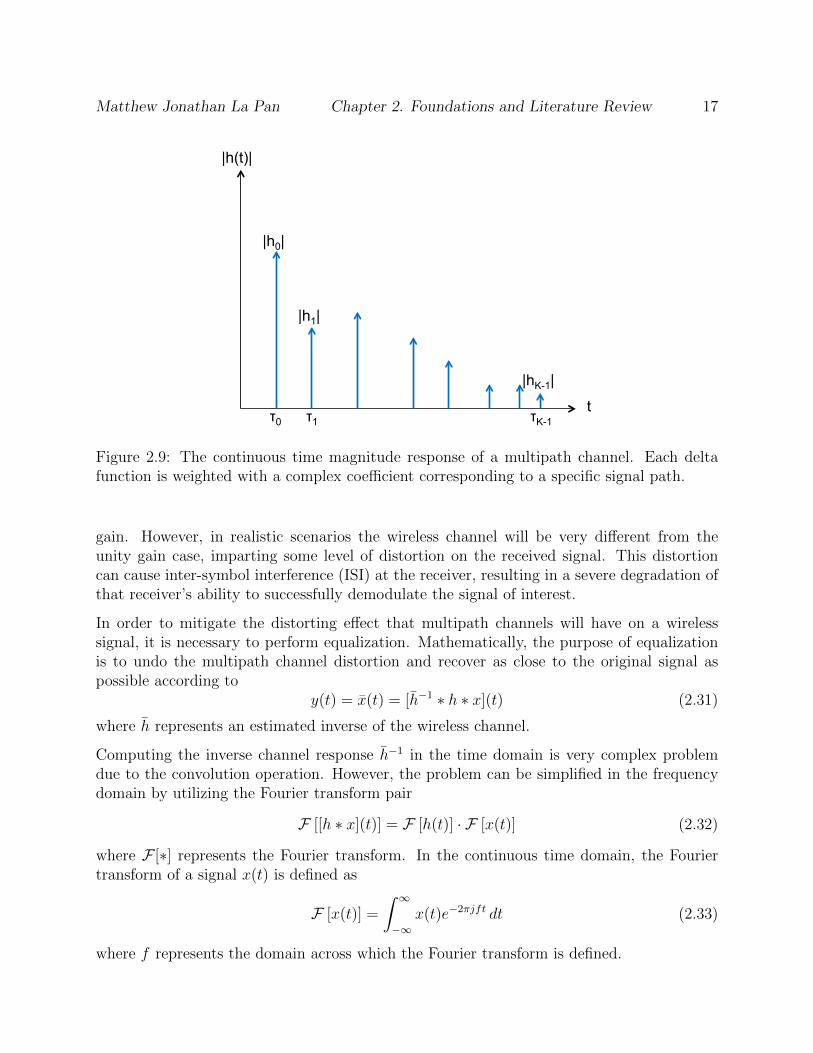
where hk ∈ C, τk ∈ [0,∞) and K represents the number of distinct signal paths from thetransmitter to the receiver. δ(t) represents the continuous time Dirac delta function. Anexample of the magnitude of a multipath channel response is shown in Figure 2.9. The signalat the wireless receiver is mathematically represented by the convolution of the transmittedsignal x(t) and the channel response according to
y(t) = [h ∗ x](t)def=
∫ ∞
−∞h(τ)x(t− τ) dτ. (2.30)
Ideally, the received signal y(t) will the same as the transmitted signal x(t). For this tooccur, it is required that h(t) = δ(t), which is often referred to as a flat channel with unity
Matthew Jonathan La Pan Chapter 2. Foundations and Literature Review 17
|h(t)|
τ0 τ1 τK-1
|h0|
|h1|
|hK-1|
t
Figure 2.9: The continuous time magnitude response of a multipath channel. Each deltafunction is weighted with a complex coefficient corresponding to a specific signal path.
gain. However, in realistic scenarios the wireless channel will be very different from theunity gain case, imparting some level of distortion on the received signal. This distortioncan cause inter-symbol interference (ISI) at the receiver, resulting in a severe degradation ofthat receiver’s ability to successfully demodulate the signal of interest.
In order to mitigate the distorting effect that multipath channels will have on a wirelesssignal, it is necessary to perform equalization. Mathematically, the purpose of equalizationis to undo the multipath channel distortion and recover as close to the original signal aspossible according to
y(t) = x(t) = [h−1 ∗ h ∗ x](t) (2.31)
where h represents an estimated inverse of the wireless channel.
Computing the inverse channel response h−1 in the time domain is very complex problemdue to the convolution operation. However, the problem can be simplified in the frequencydomain by utilizing the Fourier transform pair
F [[h ∗ x](t)] = F [h(t)] · F [x(t)] (2.32)
where F [∗] represents the Fourier transform. In the continuous time domain, the Fouriertransform of a signal x(t) is defined as
F [x(t)] =
∫ ∞
−∞x(t)e−2πjft dt (2.33)
where f represents the domain across which the Fourier transform is defined.

Matthew Jonathan La Pan Chapter 2. Foundations and Literature Review 18
Using the relationship from (2.32) in (2.31), we can see that the frequency domain represen-tation of y(t) can be represented as
Y (f) = H−1(f)H(f)X(f) (2.34)
where the uppercase notations represent the frequency domain representations of the signalsY (f) = F [y(t)], X(f) = F [x(t)] and so on. Since the goal of equalization is to mitigateany distortion in the wireless channel in order to achieve y(t) = x(t), we can see that it isdesirable for
H−1(f) =1
H(f). (2.35)
So in its most basic form, frequency domain equalization is performed on a signal by esti-mating the wireless channel and then dividing out the channel frequency response in orderto recover the undistorted signal.
This basic idea is applied to the concept of OFDM synchronization. In fact, the frequencydomain synthesis structure of OFDM lends itself to the concept of frequency domain equal-ization very well. After successful acquisition and synchronization with negligible error, anOFDM symbol can be represented as
rn =
(C−1∑
c=0
xn−do−chc
)+ nn, n = 0, 1, ..., N − 2, N − 1 (2.36)
where {do| do ∈ N, 0 ≤ do ≤ fsTcp}, meaning that the timing point is taken correctly fromsomewhere along the cyclic prefix range. This relationship is a discrete convolution of thetransmitted signal and the discrete wireless channel response plus the noise term. Applyingthe DFT to this sequence will yield
Rk = e−j2πdok/NHkXk +Nk, k = 0, 1, ..., N − 2, N − 1. (2.37)
The exponential term in this result is a linear phase shift, the frequency domain representa-tion of a uniform time shift. Based on the frequency domain equalization method discussedearlier, it is desirable for the communications system to be able to estimate the discretechannel response Hk in order to mitigate the multipath channel distortion. However, thenumber of unknown terms in (2.37) makes the channel filter response Hk difficult to estimate.
In order to estimate the channel response at the receiver, OFDM systems make use of specialcontrol symbols, usually called ’pilots’ or ’pilot tones’. These pilot tones are symbols insertedin to the data stream of an OFDM symbol in order for the receiver to make measurementsof the signal xn. These symbols are inserted in to an outgoing symbol via frequency domainsynthesis, shown in Figure 2.10. This is performed by placing specific symbols–generallyknown at the receiver–in Xk at specific, usually uniformly spaced intervals, in k. In this casethe receiver would know the sequence
Xeq = Xmp, {m|m ∈ Z,m > 1}, {p|p ∈ Z, 0 ≤ p ≤ bNmc} (2.38)

Matthew Jonathan La Pan Chapter 2. Foundations and Literature Review 19
Pilot Subcarriers Data Subcarriers
Subcarriers
… …
Figure 2.10: The use of pilot tones for OFDM equalization. The orange subcarriers are usedto transmit data to the receiver, while the green subcarriers represent the pilots used at thereceiver to take partial channel measurements for equalization. The symbols transmittedover the pilots are generally known at the receiver in order to construct a reliable channelestimate.
where m is chosen based on the coherence bandwidth
Bc ≈1
D(2.39)
whereD is the delay spread, or the amount of time between the first significant signal pathand the last. For example, in Figure 2.9 the delay spread is given by D = τK−1 − τ0. AnOFDM equalization system measures the channel via the computation
Hmp =Xmp
Rmp
(2.40)
resulting in a partial frequency domain equalization filter response of
Hko =
{1
e−j2πdok/NHk+NkXk
: k ∈ mp0 : o.w.
(2.41)
at the receiver.
A simple OFDM equalizer, called the zero forcing equalizer, interpolates the channel responseusing a low pass filter according to
Hk = Hko ∗ hLP (2.42)
which is then applied to the received signal [15]. Assuming that the channel estimation atthe receiver is accurate, the resulting frequency domain equalized signal will be
Ek =e−j2πdok/NHkXk +Nk
e−j2πdok/NHk + NkXk
. (2.43)
Matthew Jonathan La Pan Chapter 2. Foundations and Literature Review 20Frequency-Selective Fading
Symbol duration similar to or shorter than delay spread
Inter-symbol interference (ISI) Equalizer in GSM based systems
RAKE receiver in CDMA
Two-ray Rayleigh fading distribution or measured impulse responses
49
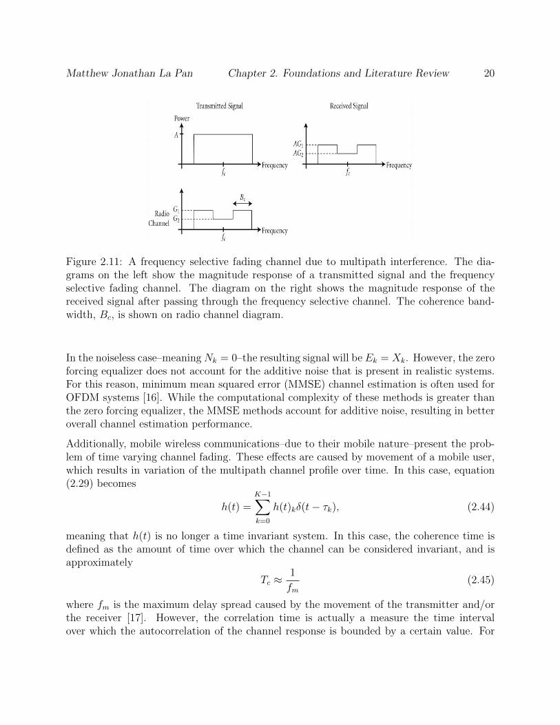
Figure 2.11: A frequency selective fading channel due to multipath interference. The dia-grams on the left show the magnitude response of a transmitted signal and the frequencyselective fading channel. The diagram on the right shows the magnitude response of thereceived signal after passing through the frequency selective channel. The coherence band-width, Bc, is shown on radio channel diagram.
In the noiseless case–meaning Nk = 0–the resulting signal will be Ek = Xk. However, the zeroforcing equalizer does not account for the additive noise that is present in realistic systems.For this reason, minimum mean squared error (MMSE) channel estimation is often used forOFDM systems [16]. While the computational complexity of these methods is greater thanthe zero forcing equalizer, the MMSE methods account for additive noise, resulting in betteroverall channel estimation performance.
Additionally, mobile wireless communications–due to their mobile nature–present the prob-lem of time varying channel fading. These effects are caused by movement of a mobile user,which results in variation of the multipath channel profile over time. In this case, equation(2.29) becomes
h(t) =K−1∑
k=0
h(t)kδ(t− τk), (2.44)
meaning that h(t) is no longer a time invariant system. In this case, the coherence time isdefined as the amount of time over which the channel can be considered invariant, and isapproximately
Tc ≈1
fm(2.45)
where fm is the maximum delay spread caused by the movement of the transmitter and/orthe receiver [17]. However, the correlation time is actually a measure the time intervalover which the autocorrelation of the channel response is bounded by a certain value. For

Matthew Jonathan La Pan Chapter 2. Foundations and Literature Review 21
example, 50% coherence time, where the autocorrelation Rhh(Tc) ≥ .5 is defined as
Tc =
√9
16π2f 2m
. (2.46)
The correlation time of a fading channel in relation to the symbol period Ts for a givenwaveform is used to characterize the channel as a fast or slow fading channel–fast fadingcorresponds to Tc < Ts and slow fading corresponds to Tc > Ts. Slow fading channelsare much more desirable because the multipath channel can be considered constant overa symbol period, as in equation (2.29), greatly simplifying channel response estimation.However, OFDM symbols have a relatively long period due to the fact that
fo =fsN. (2.47)
Combining this fact with equation (2.14) yields the result
T =1
fo. (2.48)
While single carrier modulation symbol periods are dictated by the overall bandwidth,OFDM symbol duration is dictated by the bandwidth of a single subcarrier, also referred toas the subcarrier spacing.
The fact that OFDM symbols are much longer in duration than their single carrier coun-terparts, coupled with the fact that mobile systems introduce fading channels, it is requiredthat mobile OFDM receivers perform channel estimation and equalization quite often. Gen-erally these computations are performed for every single OFDM symbol and pilot tones aretransmitted continuously. This not only adds control protocol overhead for OFDM systems,but it also presents an area for security vulnerability in OFDM systems [18, 19, 20].
While OFDM offers many advantages in terms of spectral efficiency and low cost implemen-tation, the required control processes of synchronization and equalization pose a significantsecurity vulnerability to OFDM based systems. This is not only based on the fact that bothprocesses are prerequisite to demodulation at an OFDM receiver, but that both processesare generally performed relatively often in OFDM systems with highly visible control data.In the scope of this work, we will try to understand these security vulnerabilities and proposemitigations and solutions to physical layer based security threats.
2.2 Dynamic Spectrum Access
The allocation of spectrum resources is an important topic in relation to the history andfuture of both wireless technology as well as the wireless industries. This is because of

Matthew Jonathan La Pan Chapter 2. Foundations and Literature Review 22
the fact that the amount of usable frequency spectrum for wireless technologies is limited.While the electromagnetic (EM) spectrum has not been proven to be explicitly limited by anyupper bound on frequency, the range of frequencies that are usable for communications froma technological standpoint is on the order of hundreds of gigahertz. This has put a strainon the amount of available resources as the demand for wireless applications–such as mobilebroadband–continues to grow at a breakneck pace. As the amount of available spectrum hasdwindled over past decades–illustrated in Figure 1.1–there has been an important shift inthe focus of wireless research to the emphasize the efficiency of how spectrum is utilized.
2.2.1 Time Frequency Access of the Spectrum
In order to discuss DSA problems, it is important to talk about the fundamental conceptsthat have led to the framework of DSA theory for wireless networks. While Figure 1.1 showsthe macro-division of frequency bands, the way that these resources are divided amongst mul-tiple users within a given band varies depending on the type of wireless technology employedfor a particular network. For example, some wireless systems, such as the first generationAdvanced Mobile Phone Standard, rely on dedicated channel FDMA for user resource al-location. An outline of this scheme as well as a simple diagram are provided in Section2.1. Other systems like the second generation Global System for Mobile Communication(GSM) rely on time division multiple access (TDMA) MAC layer protocol in order to divideresources amongst users. There are also standards that use code division multiple access(CDMA), like the third generation CDMA2000 family of standards. While these examplesall point out standards for cellular networks, any wireless system with multiple users requiresa multiple user access scheme for resource allocation and management amongst users.
Looking at the scope of wireless systems just in the US–based on Figure 1.1–we can see thatthere are a plethora of applications for wireless networks. Each of these networks supportsdifferent types of wireless systems with different usage patterns, and those patterns are oftendynamic. One popular example of this is the spectrum allocated to television broadcastingservices. Due to the propagation characteristics of broadcast television, frequency reuse–theconcurrent transmitting of different data over the same frequency band based on geographicalseparation–can only be performed over very large distances. This leaves a large portion ofspectral resources unused in certain locations. These allocated but unused resources aretermed white space. Both the IEEE 802.11af and 802.22 standards utilize the TV bandwhite space in order to provide mobile broadband access to end users [21, 22].
While the large amount of unutilized spectrum is good news in terms of solving the problemsposed by spectral crowding, the use of these white spaces presents a whole new set of chal-lenges for the design of wireless systems. Because the resources that are available in the whitespaces of the spectrum are already allocated to dedicated communications systems, networkswishing to access these resources have come under scrutiny for the potential interference riskthey pose to these dedicated systems [23]. Due to the complexity of this problem, wireless

Matthew Jonathan La Pan Chapter 2. Foundations and Literature Review 23
Figure 2.12: Visual comparison of three multiple access schemes. TDMA and FDMA divideuser resources in time and frequency, respectively. CDMA uses orthogonal codes that allowmultiple users to share concurrent time and frequency resources without interfering with oneanother [2].

Matthew Jonathan La Pan Chapter 2. Foundations and Literature Review 24
Figure 2.13: Example listing of available spectrum resources due to television band whitespace according to Spectrum Bridge’s Show My White Space tool. The list on the rightshows where television band devices could be used by television band devices (TVBDs).
networks that wish to utilize these white spaces require intelligent devices that can parseinformation about the surrounding RF environment in order to protect owners of licensedspectrum. This requirement has led to the idea of cognitive radios–devices that are a criticalconcept for dynamic spectrum access networks.
2.2.2 Cognitive Radio
Cognitive radio is a concept first proposed by Joseph Mitola [24] that expands upon thecapabilities of modern software defined radios. Software radios are modern devices that arecrafted to be reconfigurable, flexible devices capable of transmitting multiple waveforms.The parameters of these waveforms–including modulation type, forward error correctioncoding and frequency band to name a few–can vary greatly. This is possible because ofthe reconfigurability of the signal processing software used to handle processing in softwaredefined radios. The concept of cognitive radio expands upon the advent of software radio inthat it adds a layer of cognition and decision making capability to the device by harnessingthe processing abilities of software radio.
The cognitive engine model for cognitive radios is used to describe their intelligence archi-tecture. This architecture is based off of the OODA–observe, orient, decide and act–coinedby John Boyd. Figure 2.14 depicts a general decision flow architecture for a cognitive radiobased on the OODA loop structure. A cognitive radio will use its sensing ability to assessits RF environment. It can then use policy knowledge to orient itself to an environment

Matthew Jonathan La Pan Chapter 2. Foundations and Literature Review 25
Learn
Observe
Act Orient
Decide
Figure 2.14: Cognitive radio decision flow architecture. A cognitive radio is constantly goingthrough this loop in order to make decisions in and learn from its RF environment. Cognitiveradios have the ability to sense their surrounding spectrum and make decisions, but theyalso theoretically have the ability to learn and update their strategies and policies.
and make a decision on the best course of action–be it to transmit in a certain band, leavea certain band, frequency hop, turn down transmit power, etc. The radio can then carryout this action by reconfiguring its own software. Cognitive radios also possess a uniquecapability to learn based on the observations and previous its observations and decisions andthe impact that they have on one another.
The theoretical model of a cognitive radio lends itself to the idea of dynamic spectrum accessnetworks. Radios utilizing DSA capabilities have to be able to perform rapid sensing anddecision making in a dynamic RF environment in order to adhere to spectrum policy. Specif-ically, it is paramount that DSA radios using white space in licensed frequency bands avoidinterference to licensed users. There have been a number of works on how to best measureto this interference and perform this task [25, 26, 27, 28, 29], and recent implementationshave shown successful integration of DSA based devices in to TV white space [30, 31].
Advances in software defined radio capability through cognitive radio principles have allowedfor dynamic spectrum access schemes to become realizable for wireless systems. This has inturn led to more a more complex range of application and capability ideas for DSA networks.With the expansion of this technology comes the challenges of securing these networks frommalignant users. But in order to develop electronic warfare theory for DSA networks, itis necessary to understand the specific challenges and vulnerabilities that these networkspresent.
Matthew Jonathan La Pan Chapter 2. Foundations and Literature Review 26
Barrage Jammer
Herding Jammer
Channels Channels Channels
Channels Channels Channels Follower Jammer
Sweeping Jammer
Channels Channels Channels
Channels Channels Channels
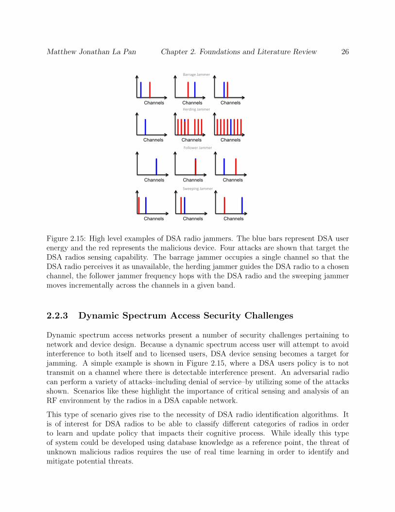
Figure 2.15: High level examples of DSA radio jammers. The blue bars represent DSA userenergy and the red represents the malicious device. Four attacks are shown that target theDSA radios sensing capability. The barrage jammer occupies a single channel so that theDSA radio perceives it as unavailable, the herding jammer guides the DSA radio to a chosenchannel, the follower jammer frequency hops with the DSA radio and the sweeping jammermoves incrementally across the channels in a given band.
2.2.3 Dynamic Spectrum Access Security Challenges
Dynamic spectrum access networks present a number of security challenges pertaining tonetwork and device design. Because a dynamic spectrum access user will attempt to avoidinterference to both itself and to licensed users, DSA device sensing becomes a target forjamming. A simple example is shown in Figure 2.15, where a DSA users policy is to nottransmit on a channel where there is detectable interference present. An adversarial radiocan perform a variety of attacks–including denial of service–by utilizing some of the attacksshown. Scenarios like these highlight the importance of critical sensing and analysis of anRF environment by the radios in a DSA capable network.
This type of scenario gives rise to the necessity of DSA radio identification algorithms. Itis of interest for DSA radios to be able to classify different categories of radios in orderto learn and update policy that impacts their cognitive process. While ideally this typeof system could be developed using database knowledge as a reference point, the threat ofunknown malicious radios requires the use of real time learning in order to identify andmitigate potential threats.

Matthew Jonathan La Pan Chapter 2. Foundations and Literature Review 27
There are a couple of methods by which a DSA radio could automatically classify otherdevices through sensing information–this problem is of great interest to both the attack andsecurity sides of the electronic warfare theory. Waveform classification and specific emitteridentification (SEI) are areas which aim to solve this problem of radio classification.
However, for DSA radios we already have a behavioral architecture from Figure 2.14 thatlends itself to stochastic classification algorithms. Due to the fact that cognitive radios withdifferent intentions have a different set of parameters controlling their decision engine, itmakes sense to use a behavior based identification system in order to classify these devices. InChapter 5, we will discuss the underlying theoretical motivation for this type of classificationmodel and show its viability even for radios with very similar decision engines.

Chapter 3
Orthogonal Frequency DivisionMultiplexing Synchronization Attacks
Orthogonal Frequency Division Multiplexing (OFDM) has become a leading modulationscheme in modern communications systems because of its spectral efficiency, achievable datarates, and robustness in multipath fading environments. However, it has been shown thatcurrent implementations of OFDM are susceptible to a variety of signal jamming attacks[18]. Various efficient jamming attacks which target the pilot tones used by OFDM commu-nications systems have been derived. While this is one aspect of communicating with OFDMwhich must be improved, it is not the only area of weakness to an intentional adversarialattack.
As discussed in Section 2.1.1, one of the most important prerequisites for communicatingusing OFDM is synchronization between the transmitter and the receiver. Both timing andfrequency synchronization are necessary in order to avoid inter-symbol interference (ISI), aswell as inter-carrier interference (ICI) and loss of orthogonality among OFDM subcarriers.A number of algorithms have been developed in order to efficiently and robustly perform thesynchronization [9, 10, 11, 12, 13].
While there has been some research conducted on analyzing and improving the robustnessof OFDM synchronization algorithms [32, 33, 34, 35, 36], the majority of this work has beenconducted under the assumption of uncorrelated or narrowband interference. In this chapter,we look at specific adversarial signals which are highly correlated to the synchronizationsymbols and designed with the intent of disrupting the communication of a transmitter andreceiver using OFDM during the synchronization stage.
28

Matthew Jonathan La Pan Chapter 3. OFDM Synchronization Attacks 29
3.1 Synchronization Model Analysis
In order to determine the relative impact that the electronic warfare tactics presented inthis paper, it is important to develop some frame of reference for the performance of OFDMsynchronization without the presence of adversarial signals. In order to do this, the followingsection analyzes the performance of the OFDM synchronization estimators in the presenceof only AWGN and multipath interference. We can then use the results from this section tomeasure the relative impact of the cognitive attacks presented in this paper.
3.1.1 Timing Acquisition Analysis
After baseband conversion and resampling, the OFDM will have a series of complex samplesthat compose the search range for the preamble symbol. These samples will be randomlyshifted in frequency subject to the clock error between the transmitter and receiver, limitedto the allowable range of offset between these two devices. We make the assumption that theoffset is approximately constant over the duration of the training sequence. The sequenceat the receiver is represented by
rn =
(C−1∑
k=0
xn−khk
)e(2πj
ffsn) + nn (3.1)
where x is the samples of the training symbol sent, h represents the impulse response ofthe channel with length C, f represents the frequency offset between the transmitter andreceiver clocks, and the term n represents noise. Substituting this term in to (2.19) yields
P (d) =L−1∑
m=0
(C−1∑
k=0
x∗d+m−kh∗ke
(−2πj ffs
(d+m)) + n∗(d+m)
)·
(C−1∑
k=0
xd+m+L−khke(2πj f
fs(d+m+L)) + nd+m+L
) (3.2)
By approximating the cross correlation terms arising from the noise as zero, we can see that
P (d) =L−1∑
m=0
(C−1∑
k=0
x∗d+m−kh∗k
)(C−1∑
k=0
xd+m+L−khk
)e(2πj
ffsL) (3.3)
Looking at the timing plateau where d ≤ d ≤ d+(Tcp−Tch)fs, we can simplify this expressionbased on the fact that the first preamble symbol is repeated over two half symbol periods,excluding the prefix, as indicated in [14]. This means that values spaced L samples apartare identical. This means that (3.3) can be simplified to
P (d) =L−1∑
m=0
∣∣∣∣∣C−1∑
k=0
xd+m−khk
∣∣∣∣∣
2
e(2πjffsL) (3.4)

Matthew Jonathan La Pan Chapter 3. OFDM Synchronization Attacks 30
We can also use (3.1) to determine the what the receiver will estimate for R(d) based on(2.20). Examining this result along the same plateau where d ≤ d ≤ d+ (Tcp − Tch)fs
R(d) =L−1∑
m=0
(∣∣∣∣∣C−1∑
k=0
xd+m−khk + nd+m
∣∣∣∣∣
)2
(3.5)
Applying the triangle inequality for complex numbers, this becomes
R(d) ≤L−1∑
m=0
(∣∣∣∣∣C−1∑
k=0
xd+m−khk
∣∣∣∣∣+ |nd+m|)2
(3.6)
Combining this result with (2.21) and (3.4) gives us
M(d) ≥
L−1∑
m=0
∣∣∣∣∣C−1∑
k=0
xd+m−khk
∣∣∣∣∣
2
2
L−1∑
m=0
(∣∣∣∣∣C−1∑
k=0
xd+m−khk
∣∣∣∣∣+ |nd+m|)2
2 (3.7)
We subsequently define
σ2xc =
L−1∑
m=0
∣∣∣∣∣C−1∑
k=0
xd+m−khk
∣∣∣∣∣
2
(3.8)
as the total power of the entire channel affected OFDM symbol and
σ2n =
L−1∑
m=0
|nd+m|2 (3.9)
as the total noise power over one OFDM symbol period. We then utilize the fact that
2L−1∑
m=0
∣∣∣∣∣C−1∑
k=0
xd+m−khk
∣∣∣∣∣ |nd+m| ≤ 2σxcσn (3.10)
with the relationship in (3.7) to obtain
M(d) ≥ σ4xc
(σ2xc + 2σxcσn + σ2
n)2(3.11)
Rearranging terms and noting that
SNR =σ2xc
σ2n
(3.12)
produces the result
M(d) ≥ 1
(1 + 1√SNR
)4(3.13)
This lower bound gives an idea of the strength of the timing peak relative to SNR.

Matthew Jonathan La Pan Chapter 3. OFDM Synchronization Attacks 31
−40 −30 −20 −10 0 10 20 30 400
0.1
0.2
0.3
0.4
0.5
0.6
0.7
0.8
0.9
1
SNR (dB)
M(d
)
Figure 3.1: Lower bound on the peak value of the timing metric plateau relative to SNR
3.1.2 Carrier Frequency Offset Estimate Analysis
Assuming a multipath channel, white Gaussian noise and correct timing acquisition, thereceived preamble after conversion to baseband can be represented as
rn =
(C−1∑
k=0
xn−khk
)e(2πj
ffsn) + nn (3.14)
where xn represents the sampled preamble symbol, hk represents a finite impulse responseapproximation of the multipath channel of length C, f represents the overall frequencyerror between the transmitter and receiver, fs is the sampling frequency, and nn representsthe sampled additive Gaussian noise. We can analyze the fine frequency estimate in orderto examine impacts of frequency domain attacks by substituting the signal as seen by thereceiver in to the equation for P (d); this yields
P (d) =L−1∑
m=0
[C−1∑
k=0
x∗d+m−kh∗ke−2πj f
fs(d+m) + n∗d+m
]·
[C−1∑
k=0
xd+m+L−khke2πj f
fs(d+m+L) + nd+m+L
].
(3.15)
This equation hinges on the assumption that the channel seen by the receiver is constant dur-ing one symbol period, an assertion that OFDM equalization is also based on. By expandingthis equation and eliminating the cross terms, P (d) approximates to
P (d) ≈L−1∑
m=0
(C−1∑
k=0
x∗d+m−kh∗ke−2πj f
fs(d+m)
)·(C−1∑
k=0
xd+m+L−khke2π f
fsf(d+m+L)
). (3.16)

Matthew Jonathan La Pan Chapter 3. OFDM Synchronization Attacks 32
Coupling the assumption that a correct timing point is taken with the fact that the firstpreamble symbol repeats itself at a spacing of L samples over all the correct timing points,this equation becomes
P (d) ≈L−1∑
m=0
∣∣∣∣∣C−1∑
k=0
xd+m−khk
∣∣∣∣∣
2
e2πjffs
(L). (3.17)
Equation (3.17) portrays the dominant term of the term P (d) at any of the correct timingpoints. Noting that this result is in phasor form, along with the fact that
L =1
2Tfs (3.18)
it is clear that the fractional frequency offset of the preamble symbol will be ∆f ≈ frac{f}.Since the exponential term can be divided in to two terms
eπjTf = eπjT frac{f}eπjint{f} = ±eπjT frac{f}. (3.19)
This term provides the fractional frequency offset only. The ambiguity due to the integerportion of the frequency offset can be disregarded as long as the partial frequency offsetis always corrected in the same direction. The coarse frequency correction process willcorrect for the remaining frequency offset. The symbols can then be multiplied by a complexexponential to correct for the fine frequency error. In the frequency domain this representsthe subcarriers being properly aligned in to bins. Once the fine frequency offset has beencomputed and corrected for, the frequency domain result will be the original symbol, with afrequency shift of an integer number of bins.
Once the fine frequency offset estimate is obtained and corrected for by multiplication of acomplex exponential, the coarse frequency offset must be computed according to equation(2.23). The terms R1,k and R2,k represent the FFT of the first and second preamble symbolsamples taken at the receiver after fine frequency correction, and are defined as
Ri,k =2L−1∑
n=0
rn+N(i−1)e−2πjkn/2L, (3.20)
where
N = fsTwp2
(3.21)
represents the number of samples in half of the preamble symbol period Twp, which includesthe cyclic prefix. Assuming perfect fine frequency correction, the received samples rn arerepresented by
rn =
(C−1∑
k=0
xn−khk
)e(2πj
int(f)fs
n) + nn. (3.22)

Matthew Jonathan La Pan Chapter 3. OFDM Synchronization Attacks 33
The first term in (3.22) is an approximation of the discrete convolution of the channel and thesignal output by the transmitter. The length C in (3.22) and the complex weights hk dependon the characteristics of the multipath channel. The channel affected signal is multipliedwith a phase shift where int(f) is an integer value corresponding to the remaining coarsefrequency shift and uncorrelated noise is added.
Based on the structure of the preamble
|X1,k|2 =
{p2 : k ∈ Y0 : k /∈ Y (3.23)
and
|X2,k|2 =
{12p2 : k ∈ B
0 : k /∈ B (3.24)
where Y is the subset of X which contains all even or odd subcarriers not part of the guardinterval. B is the subset of all of the subcarriers excluding the guardband. The term p2
is a constant proportional to the transmitted power of the preamble. The power on eachsubcarrier is halved for the second preamble symbol since it occupies both even and oddsubcarriers. We also define
|Nk|2 = p2n (3.25)
as the noise power over each OFDM subcarrier, which is assumed to be a constant. Wedefine the total signal power of one preamble symbol at the receiver as
σ2xc =
∑
k∈X
|Hk|2|X1,k|2 =∑
k∈A
|Hk|2|X2,k|2, (3.26)
where the set A represents all subcarriers, and the total noise power over one symbol as
σ2n =
∑
k∈A
|Nk|2. (3.27)
By combining (3.23) with equations (2.23) and (2.24) with the fact that, we see that
B(g) =
∣∣∑k∈X R
∗1,k+2gX1,kX
∗2,kR2,k+2g
∣∣2
p4(∑
k∈X |R2,k|2)2(3.28)
Incorporating equations (3.20) and (3.22) in the coarse offset estimator yields
B(g) =
∣∣∑k∈X (H∗k−f+2gX
∗1,k−f+2g +N∗1,k)X1,kX
∗2,k(X2,k−f+2gHk−f+2g +N2,k)
∣∣2
p4(∑
k∈X |X2,k−fHk−f +Nk|2)2 (3.29)

Matthew Jonathan La Pan Chapter 3. OFDM Synchronization Attacks 34
We can expand the numerator and rearrange the summations to show that∣∣∣∣∣∑
k∈X
|Hk−f+2g|2X1,kX∗1,k−f+2gX2,k−f+2gX
∗2,k
+∑
k∈X
X2,k−f+2gX∗2,kX1,kHk−f+2gN
∗1,k
+∑
k∈X
X1,kX∗1,k−f+2gX
∗2,kH
∗k−f+2gN2,k
+∑
k∈X
X1,kX∗2,kN
∗1,kN2,k
∣∣∣∣∣
2
.
(3.30)
Due to the uncorrelated nature of the noise, the first term of the numerator will dominate.Therefore, it is reasonable to make the approximation that
B(g) ≈∣∣∑
k∈X |Hk−f+2g|2X1,kX∗1,k−f+2gX2,k−f+2gX
∗2,k
∣∣2
p4(∑
k∈X |X2,k−fHk−f +Nk|2)2 , (3.31)
noting that the numerator is only affected by the non-zero set of subcarriers Y which arenot in the guardband.
There are two cases to consider regarding equation (3.30). The first scenario to analyze iswhen 2g = f . In this case (3.31) becomes
B(g) ≈∣∣∑
k∈X |Hk|2|X1,k|2|X2,k|2∣∣2
p4(∑
k∈X |X2,k−fHk−f +Nk|2)2 (3.32)
which, according to (3.24), simplifies to
B(gmax) =
∣∣12
∑k∈Y |Hk|2|X1,k|2
∣∣2(∑
k∈X |X2,k−fHk +Nk|2)2 (3.33)
or
B(gmax) =
(12σ2xc
)2(∑
k∈X |X2,k−fHk +Nk|2)2 . (3.34)
The triangle inequality for complex numbers shows that
|X2,k−fHk +Nk| ≤ |X2,k−fHk|+ |Nk|. (3.35)
Bounding the coarse frequency estimate at gmax by
B(gmax) ≥(12σ2xc
)2(∑
k∈X (|X2,k−f ||Hk|+ |Nk|)2)2 , (3.36)

Matthew Jonathan La Pan Chapter 3. OFDM Synchronization Attacks 35
then expanding, we see that
B(gmax) ≥(12σ2xc
)2(∑
k∈X |Hk|2|X2,k−f |2 + 2|Hk||X2,k−f ||Nk|+ |Nk|2)2 . (3.37)
Utilizing the fact that
∑
k∈X
|Hk||X2,k−f ||Nk| ≤√∑
k∈X
|Hk||X2,k−f |2∑
k∈X
|Nk|2, (3.38)
we slightly relax the bound so that (3.37) takes the form
B(gmax) ≥(12σ2xc
)2(
12
(σ2xc + 2
√σ2xcσ
2n + σ2
n
))2 . (3.39)
Based on the definition
SNR =σ2xc
σ2n
, (3.40)
this equation results in the relationship
B(gmax) ≥1
(1 + 1√
SNR
)4 . (3.41)
This bound yields an idea of how strong we can guarantee the peak of the coarse frequencycorrelation to be.
The second scenario is when 2g 6= f , meaning that the coarse frequency estimate is incorrect.In this scenario, the values of X1,k and X2,k are an independent and identically distributed se-quence of random variables. Specifically, we assume these values to be distributed accordingto
Xi,k =p√
2iCi,k + jDi,k, i = 1, 2; k ∈ Y , (3.42)
whereCi,k = 2Ai,k − 1, Di,k = 2Bi,k − 1, (3.43)
and
Ai,k, Bi,k ∼ Bern(1
2). (3.44)
The channel frequency values Hk can be modeled as a set of complex dependent Gaussianrandom variables according to
Hk = Ck + jDk, (3.45)
whereCk, Dk ∼ N (0,
pc2
). (3.46)

Matthew Jonathan La Pan Chapter 3. OFDM Synchronization Attacks 36
−40 −30 −20 −10 0 10 20 30 400
0.1
0.2
0.3
0.4
0.5
0.6
0.7
0.8
0.9
1
SNR (dB)
B(g
)
Figure 3.2: Lower bound on the coarse frequency offset estimator peak at the correct fre-quency offset relative to the effective SNR after channel fading.
The term pc represents the average power of the wireless channel across all of the activesubcarriers, specifically
pc =1
|B|∑
k∈B
|Hk|2 (3.47)
where |B| represents the size of the set |B|. Under this model, each computed channel powerspectral density value |Hk|2 will be a scaled chi-square distributed random variable accordingto
|Hk|2 ∼pc2X 2(2), (3.48)
which is equivalent to the exponential distribution
|Hk|2 ∼pc2Exp(
1
2) = Exp(
1
pc). (3.49)
This means that the interior portion of the numerator of (3.31) can be modeled accordingto
|Hk−f+2g|2X1,kX∗1,k−f+2gX2,k−f+2gX
∗2,k = Ek + jFk. (3.50)
In addition, for the product of the subcarrier symbols
X1,kX∗1,k−f+2gX2,k−f+2gX
∗2,k = Wk + jZk (3.51)
a simple variance calculation yields
V AR[Wk] = V AR[Zk] = p4. (3.52)

Matthew Jonathan La Pan Chapter 3. OFDM Synchronization Attacks 37
Due to the independence of the channel response and the frequency domain samples of thereceived signal the variance of Ek and Fk will be
V AR[Ek] = V AR[Fk] = 2p2cp4. (3.53)
From this expression, each of these terms is summed across all of the subcarriers k ∈ X .Due to the extremely weak dependence of the random variables, we then apply the centrallimit theorem to show that
∑
k∈Y
Ek + jFk ⇒√|Y|N (0, 2p2cp
4) + j√|Y|N (0, 2p2cp
4). (3.54)
Noting that √|Y|N (0, 2p2cp
4) =√
2|Y|pcp2N (0, 1) (3.55)
we can then make the same observations as equations (3.48) and (3.49) to obtain
1
p4
∣∣∣∣∣∑
k∈X
|Hk−f+2g|2X1,kX∗1,k−f+2gX2,k−f+2gX
∗2,k
∣∣∣∣∣
2
∼ Exp(1
2|Y|p2c). (3.56)
This means that the expected value of the numerator for the case where the coarse frequencyestimate is incorrect is
E[Exp(1
2|Y|p2c)] = 2|Y|p2c = |B|p2c . (3.57)
We then note, based on our definitions in (3.26) and (3.46), that
|B|p2c =∑
k∈B
|Hk|2. (3.58)
We use equations (3.24) and (3.26) to derive
∑
k∈B
|Hk|2 =2σ2
xc
p2. (3.59)
Since the denominator for both cases will be the same, we represent the numerator of (3.39)in these terms to show (
1
2σ2xc
)2
=1
16|B|2p4cp4. (3.60)
Taking the ratio of the numerator in (3.39) and the expected value of the numerator from(3.57), we see that the ratio of the lower bound on the estimate at the correct frequency tothe expected value of the incorrect estimates is
min[B(gmax)]
E[B(g 6= gmax)]=
1
16|B|p2cp4. (3.61)

Matthew Jonathan La Pan Chapter 3. OFDM Synchronization Attacks 38
Figure 3.3: The physical jamming scenario
Converting this ratio to decibels yields
min[B(gmax)]
E[B(g 6= gmax)]dB ≈ 10 log(|B|) + 20 log(pc) + 40 log(p)− 12 dB. (3.62)
This result, combined with the lower bound from (3.41), helps to illustrate the performanceof the correlation estimator in an environment without the presence of correlated adversarialsignals.
3.2 System and Channel Model
In order to study some of the effects of adversarial signals on the OFDM synchronizationprocess, a simple model was developed to imitate a realistic physical scenario. Within thisbasic model there are three main signals involved which represent the transmitter, receiverand the jammer. The transmitter and the jammer broadcast signals x and j, which thenpass through two unique multipath channels h and k, respectively. These channels can bemodeled as finite length digital filters white Gaussian noise is added to each signal at a fixedsignal to noise ratio (SNR). The received signal is the aggregate of both the transmitterand jammer signal after the addition of channel effects and noise. In this case, the receivedvector r is
rn =
(C−1∑
k=0
xn−khk
)e(2πj
ffsn) + α
(K−1∑
i=0
jn−iki
)e(2πj
fjfsn) + nn (3.63)
where hk and ki are the impulse responses of the channel that the receiver and the jammersees, respectively, of lengths C and K. The values f and fj represent the relative frequencyoffsets of the receiver with the transmitter and the jammer, and n is a vector of whiteGaussian noise.
The power of the transmitter is assumed to be fixed, while the power output of the jammercan vary based on the attack signal. This scenario gives rise to the signal-to-jammer ratio(SJR)
SJR = 10 log(α2) = 20 log(α) (3.64)
which will be used as one metric of efficiency of an attack signal.
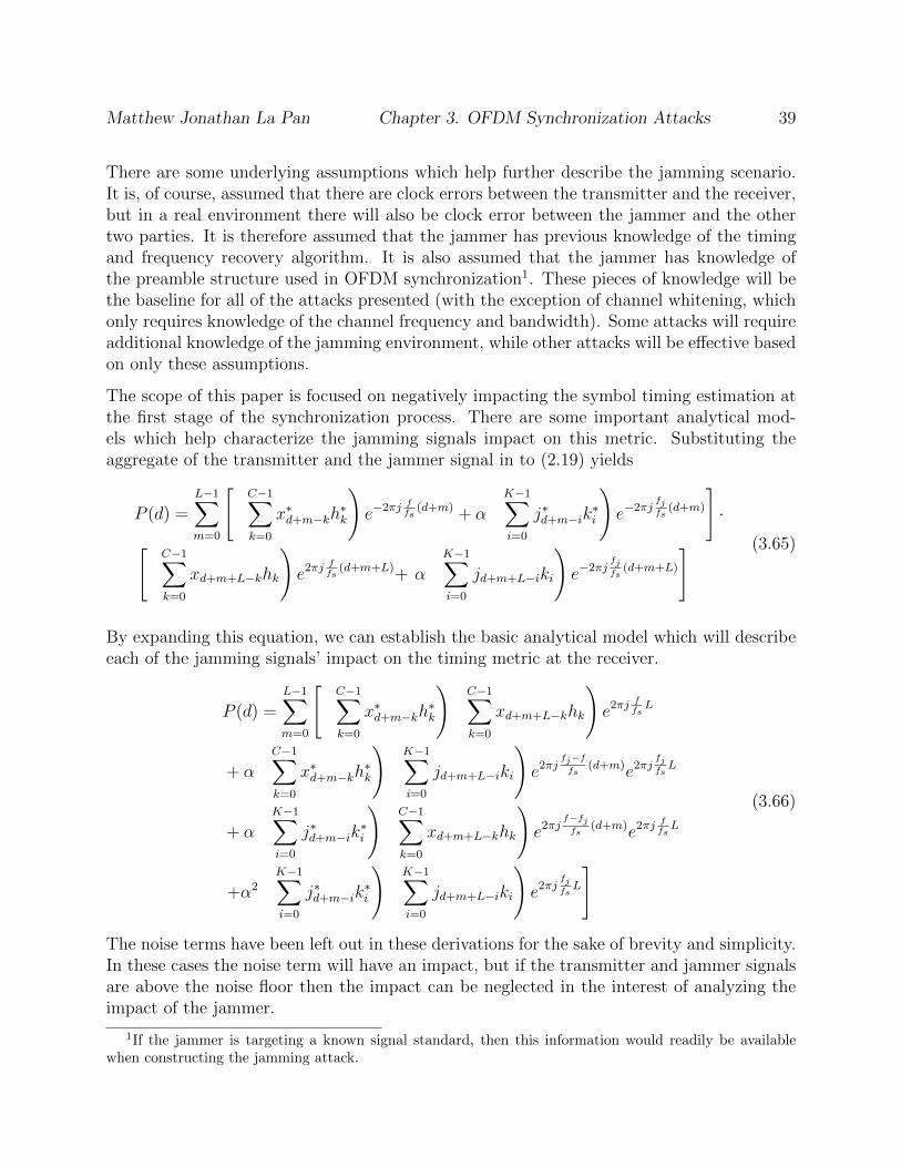
Matthew Jonathan La Pan Chapter 3. OFDM Synchronization Attacks 39
There are some underlying assumptions which help further describe the jamming scenario.It is, of course, assumed that there are clock errors between the transmitter and the receiver,but in a real environment there will also be clock error between the jammer and the othertwo parties. It is therefore assumed that the jammer has previous knowledge of the timingand frequency recovery algorithm. It is also assumed that the jammer has knowledge ofthe preamble structure used in OFDM synchronization1. These pieces of knowledge will bethe baseline for all of the attacks presented (with the exception of channel whitening, whichonly requires knowledge of the channel frequency and bandwidth). Some attacks will requireadditional knowledge of the jamming environment, while other attacks will be effective basedon only these assumptions.
The scope of this paper is focused on negatively impacting the symbol timing estimation atthe first stage of the synchronization process. There are some important analytical mod-els which help characterize the jamming signals impact on this metric. Substituting theaggregate of the transmitter and the jammer signal in to (2.19) yields
P (d) =L−1∑
m=0
[(C−1∑
k=0
x∗d+m−kh∗k
)e−2πj
ffs
(d+m) + α
(K−1∑
i=0
j∗d+m−ik∗i
)e−2πj
fjfs
(d+m)
]·
[(C−1∑
k=0
xd+m+L−khk
)e2πj
ffs
(d+m+L)+ α
(K−1∑
i=0
jd+m+L−iki
)e−2πj
fjfs
(d+m+L)
] (3.65)
By expanding this equation, we can establish the basic analytical model which will describeeach of the jamming signals’ impact on the timing metric at the receiver.
P (d) =L−1∑
m=0
[(C−1∑
k=0
x∗d+m−kh∗k
)(C−1∑
k=0
xd+m+L−khk
)e2πj
ffsL
+ α
(C−1∑
k=0
x∗d+m−kh∗k
)(K−1∑
i=0
jd+m+L−iki
)e2πj
fj−ffs
(d+m)e2πjfjfsL
+ α
(K−1∑
i=0
j∗d+m−ik∗i
)(C−1∑
k=0
xd+m+L−khk
)e2πj
f−fjfs
(d+m)e2πjffsL
+α2
(K−1∑
i=0
j∗d+m−ik∗i
)(K−1∑
i=0
jd+m+L−iki
)e2πj
fjfsL
]
(3.66)
The noise terms have been left out in these derivations for the sake of brevity and simplicity.In these cases the noise term will have an impact, but if the transmitter and jammer signalsare above the noise floor then the impact can be neglected in the interest of analyzing theimpact of the jammer.
1If the jammer is targeting a known signal standard, then this information would readily be availablewhen constructing the jamming attack.

Matthew Jonathan La Pan Chapter 3. OFDM Synchronization Attacks 40
In addition, we define the scenarios in which the jammer has channel knowledge. In thiscase, the jamming signal jn is defined as
jn = α
(K−1∑
l=0
pn−lk−1l
)e(2πj
fjfsn) (3.67)
where
pn =
(C−1∑
i=0
jn−ihi
)(3.68)
where jn is the jamming signal dependent on the attack, k−1 is the inverse jammer channelresponse such that k−1 = FFT−1(1/FFT(k)), and |α| > 0. In addition, fj represents thefrequency offset of the jamming signal at the receiver, which in most cases will be made tomatch the offset of the preamble at the receiver.
3.3 Jamming Attacks
While the synchronization process described by Schmidl and Cox can be considered robustwithin friendly communications environments, there are many weaknesses to the algorithmwere it to be intentionally and intelligently attacked. These jamming strategies allow adver-saries to be efficient relative to simple channel whitening. Even based on the importance oftiming and frequency recovery alone, a more efficient attack than channel whitening presentsitself as whitening only during preamble transmission. Some of the potential weaknesses lieboth within the timing recovery and the frequency recovery. It is interesting to note that,while OFDM is much more sensitive to errors in the estimation of carrier frequency offsetthan symbol timing, there are still various ways in which synchronization could be disruptedby creating error in either or both values. While it is not yet clear which jamming strategywould be the most efficient against OFDM synchronization in terms of power and denialrate, there are many possible candidates.
3.3.1 Timing Acquisition Attacks
Symbol timing acquisition is generally the first stage of OFDM acquisition at a receiver. Amalicious attack against this process can effectively prevent a transmitter and receiver fromcommunicating. This section outlines a series of efficient attacks that are capable of denyingservice to an OFDM receiver by targeting the symbol timing acquisition process.

Matthew Jonathan La Pan Chapter 3. OFDM Synchronization Attacks 41
Barrage Jamming Attacks
There are two types of basic jamming attacks which perform barrage attacks. Though theyare not explicitly covered in this paper, they are important to mention as the most basicattacks against OFDM. The first is a continuous white noise jammer which aims to raise thenoise floor at the receiver in order to degrade communication. This is the most inefficient andleast intelligent jammer, and can serve as a baseline for comparing the efficiencies of otherjammers. The second type of barrage attack, preamble whitening, is slightly more efficientand intelligent, though it still relies on uncorrelated noise in order to disrupt communications.This jammer raises the noise floor only during the synchronization phase, effectively tryingto drown out the preamble symbols in order to jam the receiver.
Continuous White Noise Jamming
The continuous white noise jamming method is the most basic and inefficient attack discussedin this paper. It consists of transmitting white noise across the entire bandwidth of theOFDM channel at a power such that the noise floor at the receiver is too high for anycommunication to occur. The effects of this jammer will not show up in the analyticalmodel of the timing metric, due to the uncorrelated nature of the white noise. Instead, thisbarrage jammer will degrade the effective SNR at the receiver, preventing the receiver fromever obtaining the preamble symbols, or any OFDM symbols for that matter. The requiredtransmit power of this attack will be a direct function of the OFDM transmitter power andthe required SNR at the receiver for demodulation.
Preamble Whitening
This attack is identical in concept to the previous barrage attack, except that instead ofcontinuously jamming an OFDM channel with white noise, the jammer in this scenarioonly focuses on the preamble symbols. Using this attack will improve upon the efficiencyof a jammer proportional to the size of the frames sent out by the transmitter. Sincethe preamble symbols are sent out at the beginning of each frame, this jammer aims toprevent the receiver from ever synchronizing properly with the transmitter, causing massivedegradation in the overall throughput of the system. This attack requires the knowledge ofthe preamble structure. Due to the distinct format of the preamble symbols used in thissynchronization algorithm, it would not require a particularly sophisticated jamming systemto be able to lock on to the preamble symbols and disable communication with this attack.
This attack does improve temporal efficiency, but the power requirement of the attack isstill significant. Figure 3.4 shows that the required power output by a jammer to impacttiming estimation can be significant. The timing estimate is not adversely affected by AWGNuntil the SNR drops below -10 dB. As an alternative, efficient jammers can offer superior

Matthew Jonathan La Pan Chapter 3. OFDM Synchronization Attacks 42
−50 −40 −30 −20 −10 0 100
0.1
0.2
0.3
0.4
0.5
0.6
0.7
0.8
0.9
1
SNR (dB)
Tim
ing
Err
or
Ra
te
Figure 3.4: Timing estimate error as a function of the effective SNR at the receiver.
performance degradation to OFDM signals at much lower jammer powers by exploiting theinherent features of OFDM.
These barrage attacks can still provide a useful baseline for jammer efficiency. In a sce-nario where an OFDM transmitter and receiver synchronize once every n symbols, preamblewhitening will offer a savings of
Psav = 10 log(nPcwPpw
) dB (3.69)
in transmit energy compared with what a continuous white noise jammer would require.Pcw is defined as the average transmit power of the continuous white noise barrage jammerand Ppw is the average transmit power of the preamble whitening jammer. These terms willdepend on the average power requirements of each jammer to accomplish its individual goal.This, of course, comes at the cost of the preamble whitener being able to sense and/or predictwhen the transmitter and receiver are attempting to perform synchronization. In general,the more efficient that these jammers become, the more cognition and implicit knowledge ofOFDM systems they require.
False Preamble Timing Attack
The main opportunities to efficiently disrupt symbol timing estimation lie within eithermoving the peak of the timing metric, or destroying it altogether. The first method is tocreate a new timing metric peak. Based on the knowledge that the jammer has about thepreamble, this can either be a retransmission of the preamble, a different preamble symbolaltogether or the transmission of the correct preamble at the incorrect time. If the false

Matthew Jonathan La Pan Chapter 3. OFDM Synchronization Attacks 43
timing preamble is transmitted at a higher power, then the peak of the overall timing metricwill be taken at the wrong place, and can destroy the symbol timing estimation.
The impact of this attack on the timing metric can be derived via (3.66). In this case, theattack signal can either be a copy of the preamble sent by the transmitter, or more generallycan be a preamble symbol constructed with any PN sequence. The only requirement is thatthe jamming signal be of the preamble form. For this general case, the resulting timingmetric numerator that the receiver sees will take the form
P (d) =L−1∑
m=0
∣∣∣∣∣C−1∑
k=0
xd+m−khk
∣∣∣∣∣
2
+ α
(C−1∑
k=0
x∗d+m−kh∗k
)(K−1∑
i=0
jd+m−iki
)
+ α
(K−1∑
i=0
j∗d+m−ik∗i
)(C−1∑
k=0
xd+m−khk
)+α2
∣∣∣∣∣K−1∑
i=0
jd+m−iki
∣∣∣∣∣
2
2 (3.70)
From this point there are two main cases: when the two preambles overlap and whenthey do not. We assume that the jamming symbol is sent so that there is significantseparation between its timing metric plateau and the preamble’s, specifically such that{N ∈ R | |N | > Tcpfs} where N is the delay of the false preamble relative to the correctone. This is the optimal strategy for the jammer to make the receiver miss the timing point.
The first case is based around when |N | > Tsymfs and there is no overlap between the timingpreamble symbols. This will simplify (3.70) to
P (d) =L−1∑
m=0
∣∣∣∣∣C−1∑
k=0
xd+m−khk
∣∣∣∣∣
4
+ α4
∣∣∣∣∣K−1∑
i=0
jd+m−iki
∣∣∣∣∣
4
(3.71)
From here, we incorporate the lower bound from (3.13) and split the two plateaus to showthat
M(d) >
{1
(1+ 1SNR
)2: d ∈ D
1(1+ 1
α2JNR)2
: d ∈ D −N (3.72)
where D represents the range of the timing metric plateau for the preamble, D−N representsthat range shifted by the delay N of the false preamble and JNR represents the jammer tonoise ratio determined by the symbol and jammer channel but independent of α.
The second case is when Tcpfs < |N | < Tsymfs such that the two preambles overlap. In thiscase, the two cross terms are a factor since the signals overlap in time. However, the termsrepresent single points in the cross correlation between the two preambles. If the jammerhas no channel information and the symbols are independent, then they approximate to zeroeither way. However, the case where the jammer has channel knowledge and sends the samesymbol as the transmitter requires further analysis. In this case the numerator of the timing

Matthew Jonathan La Pan Chapter 3. OFDM Synchronization Attacks 44
metric becomes
P (d) =L−1∑
m=0
∣∣∣∣∣C−1∑
k=0
xd+m−khk
∣∣∣∣∣
2
+ α
(C−1∑
k=0
x∗d+m−kh∗k
)(C−1∑
k=0
xd−N+m−khk
)
+ α
(C−1∑
k=0
x∗d−N+m−kh∗k
)(C−1∑
k=0
xd+m−khk
)+α2
∣∣∣∣∣C−1∑
k=0
xd−N+m−khk
∣∣∣∣∣
2
2 (3.73)
In order to analyze this equation we define Ry(d)y(d)(l) as the autocorrelation function
Ry(d)y(d)(l) =L−1∑
m=0
yd+my∗d+m−l (3.74)
where y(d) represents the function of interest and l is the lag between the two functions. Ifwe define
yd+m =C−1∑
k=0
xd+m−khk (3.75)
then (3.73) becomes
P (d) = Ry(d)y(d)(0) + αRy(d−N)y(d−N)(−N)
+ αRy(d)y(d)(N) + α2Ry(d−N)y(d−N)(0)(3.76)
In order to accurately compute these terms, knowledge about the autocorrelation functionof both the OFDM signal and the channel are necessary, as suggested in [37]. The autocor-relation of the OFDM symbol can be derived based on the power spectral density (PSD) viathe Einstein-Wiener-Khinchin Theorem. This is based on the fact that an OFDM signal iscyclostationary. The PSD of an OFDM symbol is a rectangular function over all subcarriersother than the guardband. The autocorrelation of an OFDM symbol is simply the inverseFourier transform of its PSD. The resulting PSD of an OFDM symbol is therefore a relativelynarrow sinc function, whose width is proportional to the size of the guardband in a partic-ular implementation. This can be seen in Figure 3.5, where the computed autocorrelationof half of the timing preamble symbol is shown, after the stripping of the cyclic prefix. Theautocorrelation function has a narrow main peak and does not show significant correlationanywhere other than zero lag. The channel autocorrelation can be estimated with a 0th orderBessel function using the Jakes’ model. Based on this modeling, it can be shown that thecross correlation terms have a relatively small impact on the peak of the timing metric, sothe numerator can be represented as
P (d) ≈ Ry(d)y(d)(0) + α2Ry(d−N)y(d−N)(0) (3.77)

Matthew Jonathan La Pan Chapter 3. OFDM Synchronization Attacks 45
The most interesting case for the overlapping scenario is when |N | = L. In this case thenumerator will take the form
P (d) = Ry(d)y(d)(0) + αRy(d±L)y(d±L)(±L)
+ αRy(d)y(d)(∓L) + α2Ry(d±L)y(d±L)(0)(3.78)
which, based on the preamble structure, becomes
P (d) = (1 + α)Ry(d)y(d)(0) + α(1 + α)Ry(d±L)y(d±L)(0) (3.79)
This result will create two different scenarios for the timing metric plateau based on thenormalization term R(d), dictated by N = L,−L.
M(d) >
{1
(1+α)2(1+ 1SNR
)2: d ∈ D,N = L
(1+α)2
α2(1+ 1JNR
)2: d ∈ D −N,N = L
(3.80)
M(d) >
{1+α
(1+ 1SNR
)2: d ∈ D,N = −L
α2
(1+α2)(1+ 1JNR
)2: d ∈ D −N,N = −L (3.81)
This result shows that the an optimal strategy for the false preamble jammer is to trans-mit with a delay equal to L. This maximizes the power normalization term R(d) withoutcontributing to the timing metric peak in P (d) caused by the transmitter’s preamble. Thislowers the bound on the timing metric peak M(d). While all delay values L ≤ N ≤ 2L willhave this effect, the delay N = L maximizes it. In addition, this effect will still make animpact even without channel or symbol knowledge.
Preamble Nulling Attack
Another method for degrading symbol timing would be to destroy the timing symbol byinversion. This attack would be carried out by a technique called preamble nulling. Thisattack would be predicated on the fact that the jammer has perfect knowledge of the preambleas viewed by the receiver. By inverting the preamble symbol in time a jammer would be ableto destructively interfere with the preamble at the receiver, wiping out the timing metricpeak. However, this method is also dependent on the relationship between the channel thatthe transmitter sees and the channel that the jammer sees. If these channels are the sameor similar enough, or if both are known to the jammer, then this attack can be effective.Without knowledge of these underlying conditions the attack becomes less feasible.
The analytical impact of this jammer can also be derived using the relationships in equations(3.66)-(3.68). The nulling jammer is sent by making jn = −xn and fj = f . Substituting the
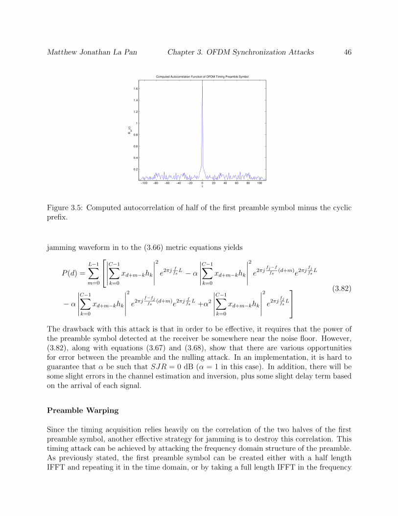
Matthew Jonathan La Pan Chapter 3. OFDM Synchronization Attacks 46
−100 −80 −60 −40 −20 0 20 40 60 80 100
0.2
0.4
0.6
0.8
1
1.2
1.4
1.6
τ
Rxx(τ
)
Computed Autocorrelation Function of OFDM Timing Preamble Symbol
Figure 3.5: Computed autocorrelation of half of the first preamble symbol minus the cyclicprefix.
jamming waveform in to the (3.66) metric equations yields
P (d) =L−1∑
m=0
∣∣∣∣∣C−1∑
k=0
xd+m−khk
∣∣∣∣∣
2
e2πjffsL − α
∣∣∣∣∣C−1∑
k=0
xd+m−khk
∣∣∣∣∣
2
e2πjfj−ffs
(d+m)e2πjfjfsL
− α∣∣∣∣∣C−1∑
k=0
xd+m−khk
∣∣∣∣∣
2
e2πjf−fjfs
(d+m)e2πjffsL +α2
∣∣∣∣∣C−1∑
k=0
xd+m−khk
∣∣∣∣∣
2
e2πjfjfsL
(3.82)
The drawback with this attack is that in order to be effective, it requires that the power ofthe preamble symbol detected at the receiver be somewhere near the noise floor. However,(3.82), along with equations (3.67) and (3.68), show that there are various opportunitiesfor error between the preamble and the nulling attack. In an implementation, it is hard toguarantee that α be such that SJR = 0 dB (α = 1 in this case). In addition, there will besome slight errors in the channel estimation and inversion, plus some slight delay term basedon the arrival of each signal.
Preamble Warping
Since the timing acquisition relies heavily on the correlation of the two halves of the firstpreamble symbol, another effective strategy for jamming is to destroy this correlation. Thistiming attack can be achieved by attacking the frequency domain structure of the preamble.As previously stated, the first preamble symbol can be created either with a half lengthIFFT and repeating it in the time domain, or by taking a full length IFFT in the frequency

Matthew Jonathan La Pan Chapter 3. OFDM Synchronization Attacks 47
domain where every other subcarrier is populated with a PN sequence. These methodsare mathematically equivalent, so either one will result in a frequency domain representationwhere every other FFT bin is empty before the addition of the cyclic prefix. The idea behindthe preamble warping attack is to transmit on the unused subcarriers of the preamble symbolin order to destroy time domain correlation.
Preamble warping essentially transforms the first symbol of the preamble in to a genericpreamble symbol, albeit that the PN sequence is still present over one half-set of the sub-carriers. By populating the unused subcarriers during timing acquisition, the attack aims todestroy timing correlation, causing the receiver to miss the timing point.
Analytically, the impact of the attack is actually better described starting from (3.66). In thecase of the warping attack, the jamming signal will have the same form as the first preamblesymbol. It is sent at the receiver frequency, but shifted over one frequency bin, such that
rn =
(C−1∑
k=0
xn−khk
)e(2πj
ffsn) + α
(K−1∑
i=0
jn−iki
)e(2πj(
ffs
+ 12L
)n) + nn (3.83)
Applying this result to the numerator of the timing metric, while once again disregardingthe noise term, yields
P (d) =L−1∑
m=0
∣∣∣∣∣C−1∑
k=0
xd+m−khk
∣∣∣∣∣
2
e2πjffsL + α
(C−1∑
k=0
x∗d+m−kh∗k
)(K−1∑
i=0
jd+m+L−iki
)e2πj
ffsLeπj
1L(d+m+L)
+ α
(K−1∑
i=0
j∗d+m−ik∗i
)(C−1∑
k=0
xd+m+L−khk
)e2πj
ffsLe−πj
1L(d+m+L) +α2
∣∣∣∣∣K−1∑
i=0
jd+m−iki
∣∣∣∣∣
2
e2πjffsLeπj
(3.84)
factoring out the constant phase term, using the time repetition properties of both sequencesand noting that the middle terms are complex conjugates yields
P (d) =L−1∑
m=0
∣∣∣∣∣C−1∑
k=0
xd+m−khk
∣∣∣∣∣
2
+ 2αRe
[(C−1∑
k=0
x∗d+m−kh∗k
)(K−1∑
i=0
jd+m−iki
)eπj
1L(d+m+L)
]
−α2
∣∣∣∣∣K−1∑
i=0
jd+m−iki
∣∣∣∣∣
2 e2πj
ffsL
(3.85)
The middle term represents a randomly phase shifted correlation between the transmittersymbol and the jammer symbol, which has an expected value of zero. Combining this with

Matthew Jonathan La Pan Chapter 3. OFDM Synchronization Attacks 48
the fact that the definition in (3.8) produces
P (d) = σ2xc − α2σ2
jk (3.86)
For cases where σ2xc and σ2
jk are close in value, it is optimal for the jammer to set α = 1.This result shows that a jammer using this attack should adjust the value of α in order tomatch the power of the transmitted symbol at the receiver in order for this attack to bemost effective. It also indicates that a scenario where the jammer has channel knowledgebut does not use the exact same symbol as the transmitter is optimal. This way, the powerterms for each of the symbols will be closest in value and the cross terms will still have anexpected value of zero.
3.3.2 Carrier Frequency Offset Estimation Attacks
Carrier frequency offset estimation is the process by which an OFDM receiver mitigates theclock errors between itself and a transmitter. A malicious attack against this process cancause massive ICI, also destroying communication between a transmitter and receiver. Thissection outlines a series of efficient attacks that are capable of denying service to an OFDMreceiver by targeting the carrier frequency offset estimation.
In order to measure the effectiveness of the attacks in this section, the root mean squared(RMS) error between the true frequency offset and the frequency offset estimation will serveas a metric for the effectiveness of the jamming attacks. This error is calculated as
eRMS =√< (foff − fest)2 >, (3.87)
where < · > is the mean, and will measure the accuracy of the frequency offset estimate.
This metric is important because it directly ties in with the degradation of SNR at thereceiver, and subsequently synchronization system performance. This is because OFDMsystems begin to suffer noticeable degradations in SNR for frequency offsets that are as littleas 1% of the subcarrier spacing [7]. Based on the work done in [8], the degradation in SNRin dB at the receiver based on carrier frequency offset can be expressed as
D ≈ 10
3ln(10)(π
∆F
F)2EsNo
. (3.88)
The term ∆F is defined as the frequency offset at the receiver, and the term F signifiesthe subcarrier or bin spacing in the OFDM symbols. The degradation is proportional tothe Es/No at the receiver, the ratio of energy per symbol to noise spectral density. Thisapproximation assumes that the frequency offset is small relative to the bin spacing. Figure3.6 illustrates the degradation in SNR for OFDM symbols based on the relative frequencyoffset using different digital modulations on the subcarriers. Using the marginal values for

Matthew Jonathan La Pan Chapter 3. OFDM Synchronization Attacks 49
−3 −2.8 −2.6 −2.4 −2.2 −2 −1.8 −1.6 −1.4 −1.2 −110
−2
10−1
100
Frequency Offset vs. SNR Degradation for OFDM Using Various Subcarrier Modulations
log(∆F/F)
De
gre
da
tio
n (
dB
)
BPSK: Es/N
o = 10.6 dB
QPSK: Es/N
o = 13.6 dB
16 − QAM: Es/N
o = 17.6 dB
64− QAM: Es/N
o = 22.1 dB
Figure 3.6: Degradation as a function of the relative frequency offset of received OFDMsymbols using various subcarrier modulations
Es/No for each of these modulations, it is clear that even slight errors in the fine frequencyoffset can have a significant impact on the effective SNR of an OFDM symbol at the receiver.This aspect of OFDM illustrates one of the glaring weaknesses of the synchronization processand highlights a definite susceptibility to adversarial signals.
Preamble Phase Warping
The first of the frequency based synchronization jamming attacks is preamble phase warp-ing. This attack aims to disrupt the frequency offset estimate of the receiver by sending afrequency shifted preamble symbol to the receiver. While it is important to note that thistype of attack could be used to change the overall frequency error estimate at the receiver,another important use of the attack would be to degrade the fine frequency estimate. Byaltering the fine frequency offset, this jamming attack can prevent the receiver from properlylining up the subcarriers in to frequency bins at the receiver. This results in massive ICIand subsequent degradation of SNR.
This attack can be analyzed using equation (3.15) by adding in the term
wn =
(K−1∑
i=0
yn−iki
)e(2πj
fjfsn) (3.89)
at the receiver. By ignoring the noise cross correlation terms as in the original derivation,

Matthew Jonathan La Pan Chapter 3. OFDM Synchronization Attacks 50
we can see that
P (d) =L−1∑
m=0
C−1∑
k=0
|xd+m−khk|2e2πjffsL + α
K−1∑
i=0
y∗d+m−ik∗i e−2πj
fjfs
(d+m)C−1∑
k=0
xd+m+L−khke2πj f
fs(d+m+L)
+ αC−1∑
k=0
x∗d+m−kh∗ke−2πj f
fs(d+m)
K−1∑
i=0
yd+m+L−ikie2πj
fjfs
(d+m+L)
+ α2
K−1∑
i=0
|yd+m−iki|2e2πjfjfsL.
(3.90)
From here, there are two cases of interest. The first is when the jammer has no channelknowledge and sends an arbitrary preamble symbol. In this case, the fine frequency estimatewill be based off of
P (d) =L−1∑
m=0
(C−1∑
k=0
|xd+m−khk|2e2πjffsL + α2
K−1∑
i=0
|yd+m−iki|2e2πjfjfsL)
)(3.91)
which results in a two polar form complex numbers. The peak autocorrelation value of thetransmitter’s symbol and channel are stochastically identical to that of the jammer’s symboland channel, so their impact on the weighting of the timing metric angle is negligible. Theresulting angle is determined according to the addition of angles of complex numbers, whichyields the equation
∠(P (d)) = arctan
(sin(2π f
fsL) + α2 sin(2π
fjfsL)
cos(2π ffsL) + α2 cos(2π
fjfsL)
). (3.92)
Given two random angles, this function versus α, which is proportional to SJR, the resultingfunction which determines the angle of P (d) is an S-shaped curve which converges towardsthe angle of the preamble at high SJRs and converges towards the angle of the jammer atlow SJRs.
The second case is when the jammer has channel knowledge and sends the same symbol asthe transmitter. In this case, the cross terms in (3.90) do not go to zero. The two crossterms between the jammer and transmitter signal are represented by the expression
L−1∑
m=0
α
(C−1∑
k=0
|xd+m−khk|2e2πjf−fjfs
(d+m)e−2πjfjfsL +
C−1∑
k=0
|xd+m−khk|2e2πj−(f−fj)
fs(d+m)e2πj
fjfsL
).
(3.93)
The termL−1∑
m=0
e2πjf−fjfs
(d+m) can be modeled as a phasor with a random angle which is de-
pendent on the jammer and transmitter frequencies and their phases at the receiver. This

Matthew Jonathan La Pan Chapter 3. OFDM Synchronization Attacks 51
−50 −40 −30 −20 −10 0 10 20 30 40 500.2
0.4
0.6
0.8
1
1.2
1.4
1.6
1.8
SJR (dB)
∠ P
(d)
Without Channel Information
With Channel Information
Figure 3.7: Estimate of the angle of P (d) at the receiver based on the SJR of the phasewarping attack with randomly generated frequency offsets. The estimate converges to thefractional frequency offset of the transmitter at high SJRs and the jammer at low SJRs.
term is represented as a = e2πjφ where φ ∼ U(0, 1). The angle of these cross terms is thendetermined by
arctan
(sin(2π( f
fs+ φ)L) + sin(2π(
fjfs− φ)L)
cos(2π( ffs
+ φ)L) + cos(2π(fjfs− φ)L)
)(3.94)
which, using sum to product identities, simplifies to
2πL
(ffs
+fjfs
)
2(3.95)
which is the average of the two signals phase offset at the receiver. Incorporating thisresult with (3.90) and (3.92) shows that the fine frequency estimate at the receiver will bedetermined according to
∠(P (d)) = arctan
(sin(2π f
fsL) + α sin(2πL
(f+fj)
2fs) + α2 sin(2π
fjfsL)
cos(2π ffsL) + α cos(2πL
(f+fj)
2fs) + α2 cos(2π
fjfsL)
). (3.96)
Figure 3.7 shows the behavior of the fine frequency estimate at the OFDM receiver whenexposed to the phase warping attack.
This attack can also be modeled stochastically based on a random frequency offset overa given range2. The frequency offset for any given system within the specified range can
2The frequency offset error for an OFDM system would have to be constrained within a specific range inorder to not interfere with adjacent channels.

Matthew Jonathan La Pan Chapter 3. OFDM Synchronization Attacks 52
be modeled as a continuous random variable with a uniform distribution over the givenfrequency range. While there may be another distribution which models this offset moreclosely, a uniform distribution is a sufficient approximation for the purposes of this paper.For the model that we used, both the receiver frequency offset, X, and the phase warp offset,Y , are chosen from uniform distributions according to
X, Y ∼ U(fLo, fHi) (3.97)
where fLo and fHi are the lowest and highest possible frequencies based on the allowableclock error for a given system.
As previously stated, frequency estimation for OFDM is extremely sensitive to the extentthat errors on the order of 1% of a subcarrier spacing can cause significant degradation to theeffective SNR at the receiver. In an ideal jamming scenario where the attacker has knowledgeof the exact preamble symbol, channel state information and frequency offset estimates, thisattack effectively randomizes the frequency estimation within the range of possible offsets3.
We can use the metric described in (3.87) to perform analysis of the ideal phase warpingattack. Incorporating the model for the frequency offset and estimation in to this equationyields
eRMS =
√< ((fRx − fTx)− (fRx − fTx))2 >. (3.98)
fTx in this equation represents the carrier frequency based on the transmitter clock, fRxrepresents the carrier frequency based on the receiver clock and fTx represents the estimateof the carrier frequency at the transmitter as made by the receiver. In this context we notethat
fRx = fTx +X. (3.99)
As shown in Figure 3.7, the receiver estimate for the phase angle will converge to the frac-tional frequency offset of the jammer at low SJRs. Equation (3.98) then converges to
eRMS =√< ((fRx − fTx)− (fRx − (fTx + Y )))2 >, (3.100)
which simplifies toeRMS =
√< Y 2 >. (3.101)
As the sample size of the measured errors becomes sufficiently large, (3.101) will converge to
eRMS =√E[Y 2]. (3.102)
Noting thatE[Y ]2 = 0, (3.103)
it follows thateRMS =
√V AR[Y ] = σ (3.104)
3The range of possible frequency offsets is something that would be constrained by the signal standard.
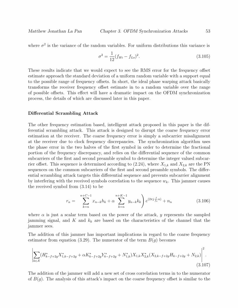
Matthew Jonathan La Pan Chapter 3. OFDM Synchronization Attacks 53
where σ2 is the variance of the random variables. For uniform distributions this variance is
σ2 =1
12(fHi − fLo)2. (3.105)
These results indicate that we would expect to see the RMS error for the frequency offsetestimate approach the standard deviation of a uniform random variable with a support equalto the possible range of frequency offsets. In short, the ideal phase warping attack basicallytransforms the receiver frequency offset estimate in to a random variable over the rangeof possible offsets. This effect will have a dramatic impact on the OFDM synchronizationprocess, the details of which are discussed later in this paper.
Differential Scrambling Attack
The other frequency estimation based, intelligent attack proposed in this paper is the dif-ferential scrambling attack. This attack is designed to disrupt the coarse frequency errorestimation at the receiver. The coarse frequency error is simply a subcarrier misalignmentat the receiver due to clock frequency discrepancies. The synchronization algorithm usesthe phase error in the two halves of the first symbol in order to determine the fractionalportion of the frequency discrepancy, and relies on the differential sequence of the commonsubcarriers of the first and second preamble symbol to determine the integer valued subcar-rier offset. This sequence is determined according to (2.24), where X1,k and X2,k are the PNsequences on the common subcarriers of the first and second preamble symbols. The differ-ential scrambling attack targets this differential sequence and prevents subcarrier alignmentby interfering with the received symbols correlation to the sequence wk. This jammer causesthe received symbol from (3.14) to be
rn =
(n+C−1∑
k=n
xn−khk + αn+K−1∑
k=n
yn−kkk
)e(2πj
ffsn) + nn (3.106)
where α is just a scalar term based on the power of the attack, y represents the sampledjamming signal, and K and kk are based on the characteristics of the channel that thejammer sees.
The addition of this jammer has important implications in regard to the coarse frequencyestimator from equation (3.29). The numerator of the term B(g) becomes
∣∣∣∣∣∑
k∈X
(H∗k−f+2gX∗1,k−f+2g + αK∗k−f+2gY
∗k−f+2g +N∗1,k)X1,kX
∗2,k(X2,k−f+2gHk−f+2g +N2,k)
∣∣∣∣∣
2
.
(3.107)
The addition of the jammer will add a new set of cross correlation terms in to the numeratorof B(g). The analysis of this attack’s impact on the coarse frequency offset is similar to the

Matthew Jonathan La Pan Chapter 3. OFDM Synchronization Attacks 54
derivation of the coarse frequency metric for the case g 6= gmax. The attack term will createanother term, J , in the coarse frequency numerator, which will be distributed according to
J ∼ α2Exp(1
2|Y|p2k) = Exp(
1
2α2|Y|p2c). (3.108)
This term will severely impact the coarse frequency estimate for significant α. The ratio ofthe numerator of the correct coarse frequency estimate to the expected value of the incorrectestimates becomes
min[B(gmax)]
E[B(g 6= gmax)]dB ≈ 10 log(|B|) + 20 log(pc) + 40 log(p)− 20 log(α)− 12 dB. (3.109)
In addition, this attack could also have an impact on the fine frequency estimate at thereceiver.
The attack is carried out by either transmitting a constant or a random stream of symbolsacross the subcarriers used in the first preamble symbol. This attack is similar in structureto the false preamble timing attack proposed in [38]. Instead, the idea behind this attack isto distort the amplitude and phase of the received subcarriers in the first preamble symbol,in turn altering the differential sequence at the receiver. The symbols transmitted by theattacker on each subcarrier are constant based on the assumption that the PN sequence ofthe first preamble symbol is unknown. Assuming the sequence is random and its symbolvalues are uniformly distributed, transmitting a constant sequence has the same probabilityof altering the phase at each subcarrier as transmitting a random symbol. Differing thissequence will degrade the performance of the coarse frequency estimation and can result insubcarrier misalignment at the receiver.
3.4 Simulation and Attack Comparison
We developed synchronization simulations in order to test the performance of current syn-chronization algorithms in the face of symbol timing attacks. The tests were performed inmultiple scenarios for each jammer in order to illustrate their individual capabilities. Theminimum knowledge requirements for each of the jammers is displayed in Table 3.4.
The results of the false preamble timing attack follow the analytical results closely. Theresults in Figure 3.8 indicates that the false preamble timing attack is extremely effective indestroying the symbol timing estimate, especially in the case where the delay, N , of the falsepreamble is equal to the timing window length L. These results indicate that a jammer couldforce the receiver to synchronize with it as opposed to the true transmitter. This representsa relatively efficient method for disrupting OFDM-based communications.
The preamble warping results also reflect the analytical results as well. The attack is mosteffective when the two symbols are transmitted at identical power, which is the more likely

Matthew Jonathan La Pan Chapter 3. OFDM Synchronization Attacks 55
Table 3.1: Situational knowledge provided to each jammer for simulation
JammingAttack
StructureSymbolTiming
FrequencyOffset Channel
FalsePreamble
Yes Window No No
PreambleNulling
Yes Exact Yes Yes
PreambleWarping
Yes Exact Yes No
−30 −20 −10 0 10 20 300
0.1
0.2
0.3
0.4
0.5
0.6
0.7
0.8
0.9
1
SJR (dB)
Tim
ing
Err
or
Ra
te
Channel Knowledge
Exact Copy w/ Channel
No Channel Knowledge
Exact Copy Delay N=L
Channel Knowledge Delay N=L
No Channel Knowledge Delay N=L
Figure 3.8: Symbol timing error rate as a function of the SJR of the false preamble timingattack.

Matthew Jonathan La Pan Chapter 3. OFDM Synchronization Attacks 56
−15 −10 −5 0 5 10 150
0.1
0.2
0.3
0.4
0.5
0.6
0.7
0.8
0.9
SJR (dB)
Tim
ing
Err
or
Ra
te
Channel Knowledge, 20 dB
Channel Knowledge, −20 dB
No Channel, −20 dB
No Channel, 20 dB
Figure 3.9: Symbol timing error rate as a function of the SJR at the receiver caused by thepreamble warping attack at an SNR of 20 dB.
when the jammer has channel knowledge. However, even in the case where the jammer hasno channel knowledge, Figure 3.9 shows that there is a significant disruption to acquisitionat the receiver, producing error rates of almost .5.
In addition, Figure 3.9 indicates that the error rate is higher at higher SJRs. This is due tothe fact that the signal power and the SNR were kept constant, while the jammer power wasvaried for comparison. This result signifies that increasing the jammer power too high willactually start to improve the timing acquisition at the receiver. This is because the warpingattack is just a frequency shifted version of the timing preamble symbol, so sending a highlypowered jamming signal will effectively increase the SNR seen at the receiver. However, thecoarse frequency estimate would likely also be hampered, but as far as the timing estimationgoes, this result is undesirable for a jammer. This is a useful result because it indicates thatjammers using a warping attack are better off erring on the side of lower power than thetransmitter signal, making this attack even more efficient.
We also developed some simulation scenarios in order to determine the impact of thesefrequency jamming attacks on OFDM synchronization. Each attack was tested under twodifferent scenarios. The first scenario is assuming that the jammers have full channel knowl-edge of both their own channel and the transmitters. This means that the jammer can senda signal
yn = α
(K−1∑
l=0
pn−lk−1l
)(3.110)

Matthew Jonathan La Pan Chapter 3. OFDM Synchronization Attacks 57
−10 −8 −6 −4 −2 0 2 4 6 8 100.1
0.2
0.3
0.4
0.5
0.6
0.7
0.8
0.9
1
SJR (dB)
Tim
ing
Err
or
Ra
te
−30 dB SNR
−20 dB
−10 dB
0 dB
10 dB
20 dB
Figure 3.10: Timing estimate error rate as a function of SJR for the preamble nulling attackat an SNR of 20 dB.
where
pn =
(C−1∑
i=0
yn−ihi
)e(2πj
fjfsn) (3.111)
and α is determined by the SJR, and the frequency shift is a determined randomly andconstrained to within a few subcarrier spacings. The term pn is the jamming signal convolvedwith the channel response of the transmitter’s channel at the given frequency offset. Theterm yn represents the scaled convolution of signal pn with k−1i , the inverse of the jammer’schannel. This means that the received jamming signal will be pn. The second scenarioassumes no channel knowledge by the jammer, so that both the transmitter and jammertransmit across distinct multipath channels. We also included a simulation of the phasewarping attack with perfect knowledge of the preamble symbol. This simulation provides abase line measurement for both the frequency estimation error rate and the RMS estimationerror. Each of these scenarios were simulated a thousand times each over a range of SJRs.
The results for the phase warping attack show that it is highly disruptive to the frequencyoffset estimation at the receiver. Errors for these simulations were considered to be offsetestimations at the receiver that were more than a tenth of a subcarrier away from their truevalue. This is more than enough estimation error to cause severe degradation to the effectiveSNR at the receiver. While the phase warping attack is extremely effective in causing errorswhen it has channel knowledge and transmits at equal or higher power as the transmitter, thephase warper with no channel knowledge actually out performs one with channel knowledgeat high SJRs.
In terms of the ideal phase warping attack, where the jammer has exact knowledge of the

Matthew Jonathan La Pan Chapter 3. OFDM Synchronization Attacks 58
−10 −8 −6 −4 −2 0 2 4 6 8 100
0.1
0.2
0.3
0.4
0.5
0.6
0.7
0.8
0.9
SJR (dB)
Fre
qu
en
cy E
rro
r R
ate
Exact Copy
Channel Knowledge
W/O Channel Knowledge
Figure 3.11: Frequency offset estimation error rate as a function of the SJR of three phasewarping attacks with varying levels of situational knowledge.
−10 −8 −6 −4 −2 0 2 4 6 8 10
1
2
3
4
5
6
7
SJR vs. RMS Frequency Error at an SNR of10 dB
SJR (dB)
RM
S E
rro
r
Exact Copy
Channel Knowledge
W/O Channel Knowledge
Figure 3.12: Frequency offset estimation RMS error as a function of the SJR of the phasewarping attack with channel knowledge.

Matthew Jonathan La Pan Chapter 3. OFDM Synchronization Attacks 59
preamble symbol, the simulations show that the less cognitive attacks perform considerablywell. The version of this attack with only OFDM standards knowledge–the least cognitive ofthese attacks–actually outperforms the idealized attack and the attack with channel knowl-edge at SJRs of 6 dB or higher. In scenarios where the jammer is transmitted at a higherpower, the advantage of channel knowledge can provide an advantage of up to 6 dB. All threevarieties of this attack seem to have certain advantages within different situations dependingon the balance between the constraints of power and complexity.
In addition to the performance metric of estimation error rate, Figure 3.12 helps to illustratesome of the underlying impacts of each of these attacks on the preamble based frequencyerror estimation process. This graph shows the RMS error of the frequency offset estimationin terms of subcarrier bins. The results from this graph give very interesting insight in to thenature of the different attacks. First of all, the RMS error for the ideal phase warping attackhighlights two important points about the synchronization process and this attacks impact.The first is that at relatively high SJRs, the ideal phase warping attack still causes significantdegradation in the success rate of frequency synchronization despite the fact that the RMSerror is extremely low (approximately .06 at an SJR of 10 dB). This speaks to the extremelysensitive nature of the frequency offset estimate. The second important result is that theerror quickly converges to the standard deviation of the random distribution of possiblefrequency offsets as previously suggested. For these simulations both the frequency offset,X, at the receiver and the warping frequency, Y , were chosen from a uniform distributionspanning five subcarrier spacing in either direction
X, Y ∼ U(−5, 5). (3.112)
Calculating the standard deviation σ from (3.105) yields an approximate standard deviationof 2.89, which is in agreement with the results from Figure 3.12.
In the cases of the non-ideal phase warping attacks the RMS errors are much different. Theattack that has full channel awareness without exact knowledge of the preamble demonstratesa similar RMS error as the ideal attack at SJRs of 0 dB or greater. However, once the powerof the jamming signal starts to exceed that of the preamble the error for the non-ideal attackwith channel knowledge continues to climb above the standard deviation for a uniformlyrandom distribution of frequency offsets within the given range. This phenomenon–whichalso shows up in the RMS error for the blind attack–can be likened to the fact that theseattacks can cause frequency estimation errors outside of the possible offsets. Fundamentally,this result suggests one of the main differences between the ideal attack and the other twoversions of this attack. When the non-ideal attacks are successful in causing the frequencyestimation process to miss, they cause it to miss bigger than the ideal attack. While theoverall error rates are not as high for these attacks, the error margins tend to be widerand more spread out than the ideal attack. This aspect of the non-ideal attacks may ormay not be desirable for the jammer, depending on factors such as the level of cognition ofthe target device. In either case, the RMS error results for all three versions of the phasewarping jammer suggest that the attack is very effective in increasing the randomness of the
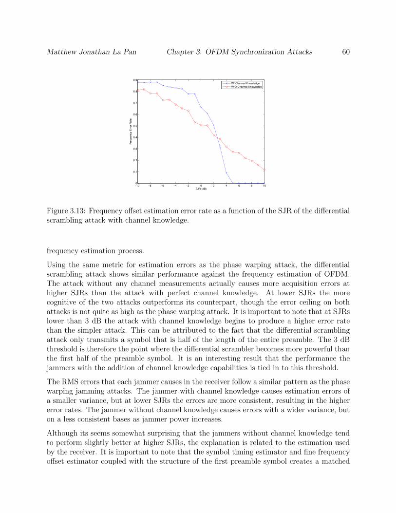
Matthew Jonathan La Pan Chapter 3. OFDM Synchronization Attacks 60
−10 −8 −6 −4 −2 0 2 4 6 8 100
0.1
0.2
0.3
0.4
0.5
0.6
0.7
0.8
0.9
SJR (dB)
Fre
quency E
rror
Rate
W/ Channel Knowledge
W/O Channel Knowledge
Figure 3.13: Frequency offset estimation error rate as a function of the SJR of the differentialscrambling attack with channel knowledge.
frequency estimation process.
Using the same metric for estimation errors as the phase warping attack, the differentialscrambling attack shows similar performance against the frequency estimation of OFDM.The attack without any channel measurements actually causes more acquisition errors athigher SJRs than the attack with perfect channel knowledge. At lower SJRs the morecognitive of the two attacks outperforms its counterpart, though the error ceiling on bothattacks is not quite as high as the phase warping attack. It is important to note that at SJRslower than 3 dB the attack with channel knowledge begins to produce a higher error ratethan the simpler attack. This can be attributed to the fact that the differential scramblingattack only transmits a symbol that is half of the length of the entire preamble. The 3 dBthreshold is therefore the point where the differential scrambler becomes more powerful thanthe first half of the preamble symbol. It is an interesting result that the performance thejammers with the addition of channel knowledge capabilities is tied in to this threshold.
The RMS errors that each jammer causes in the receiver follow a similar pattern as the phasewarping jamming attacks. The jammer with channel knowledge causes estimation errors ofa smaller variance, but at lower SJRs the errors are more consistent, resulting in the highererror rates. The jammer without channel knowledge causes errors with a wider variance, buton a less consistent bases as jammer power increases.
Although its seems somewhat surprising that the jammers without channel knowledge tendto perform slightly better at higher SJRs, the explanation is related to the estimation usedby the receiver. It is important to note that the symbol timing estimator and fine frequencyoffset estimator coupled with the structure of the first preamble symbol creates a matched

Matthew Jonathan La Pan Chapter 3. OFDM Synchronization Attacks 61
−10 −8 −6 −4 −2 0 2 4 6 8 100
1
2
3
4
5
6SJR vs. RMS Frequency Error at an SNR of10 dB
SJR (dB)
RM
S E
rro
r
W/ Channel Knowledge
W/O Channel Knowledge
Figure 3.14: Frequency offset estimation RMS error as a function of the SJR of the differentialscrambling attack with channel knowledge.
filter at the receiver since we have assumed the channel to be time-invariant over the periodof the preamble. This means that–outside of noise–the estimated values at the receiverare much more deterministic for a given channel. In the case where the jammer and thetransmitter see different channels, there receiver is not a matched filter for the cross termsbetween the two signals. This effect causes randomness in the numerator of the estimators,while the power normalization terms in the denominators still reflect the total power of boththe jammer and transmitter preamble. This phenomenon seems to have the most impactspecifically when both of these signals are transmitted with equal power.

Chapter 4
Attack Mitigation
Both OFDM timing and frequency synchronization are necessary in order to avoid inter-symbol interference (ISI), as well as inter-carrier interference (ICI) and loss of orthogonalityamong OFDM subcarriers. In addition, this process must be performed often in order toensure accurate tracking of timing and frequency offsets between a transmitter and a receiver.A number of algorithms have been developed in order to efficiently and robustly perform thesynchronization [14, 39, 40, 9, 10, 11, 12, 13].
However, as we have shown in previous sections, there are still many shortcomings of OFDMsynchronization in the presence of efficient adversarial devices. It has been shown thatcurrent implementations of OFDM are susceptible to a variety of pilot jamming attacks[18]. There has been research conducted on analyzing and improving the robustness ofOFDM synchronization algorithms under interference conditions [41, 8, 32, 33, 34, 35, 36],as well as on the performance of existing OFDM synchronization algorithms in the presenceof targeted jamming attacks [42, 38, 43]. These works underscore the theme that OFDMimplementations often require multiple, flexible security features in order to be robust.
In addition, due to the importance of OFDM synchronization and the high frequency atwhich it is calculated in realistic systems, it is important to develop algorithms that areefficient while still being secure. In this chapter, we present a novel method for performingOFDM synchronization utilizing the well known cross ambiguity function (CAF). We analyzethe validity of this method for computing the timing point and carrier frequency offsetin an OFDM system in addition to the CAF’s performance in a realistic communicationsenvironment with multipath fading. In addition, we discuss how this synchronization methodcan be used in conjunction with a technique called ’sync-amble’ randomization in order tovastly improve the overall security of the OFDM synchronization process.
62

Matthew Jonathan La Pan Chapter 4. Attack Mitigation 63
4.1 Cross Ambiguity Function Based Orthogonal Fre-
quency Division Multiplexing Acquisition
The first improvement to physical layer security proposed in this paper is based on usingthe Cross Ambiguity Function (CAF) to compute the timing point and frequency offsetestimation at the OFDM receiver. The main advantage of performing synchronization usingthe CAF is that it does not require an easily identifiable, time repetitive symbol as in[14]. The synchronization symbol will still have a cyclic prefix, but will not be physicallydiscernible from any data bearing OFDM symbol.
4.1.1 Theoretical Analysis of Synchronization with the AmbiguityFunction
Assuming that the synchronization symbol sent resembles an ordinary data symbol, and thatthe channel from the transmitter to the receiver can be modeled as an AWGN multipathchannel with finite length impulse response, the sampled signal at the receiver after basebandconversion is represented as
rn =
(C−1∑
k=0
xn−d−khk
)e2πj
ffsn + nn (4.1)
where the subscript n represents the sample index and spans the search area for the trainingsymbol, d is the delay value and timing point of the symbol, C is the length of the channelapproximation, f represents the carrier frequency offset and n is the noise term.
Since the receiver will not be able to use a delay line correlation as a matched filter forsynchronization, it is required that the receiver have the baseband signal, xn, of the OFDMtraining symbol in memory. This signal is the same as the one in (4.1), except that there isno frequency offset term and its length is exactly that of the training sequence, as opposed tothe range that the receiver is searching. This means that the CAF method synchronizationsymbol will physically resemble any other data bearing OFDM symbol.
The receiver will then compute the CAF using the received baseband signal and the localbaseband signal according to
A(u, v) =
∣∣∣∣∣N−1∑
k=0
xkr∗k+ue
−2πjkv/N
∣∣∣∣∣ (4.2)
where r and x represent the low pass equivalents of the two sampled copies of a given signal,u and v represent the timing and frequency offsets in terms of samples and frequency bins,respectively, where 0 ≤ u ≤ dmax and |v| ≤ Nfmax/fs. N represents both the length in

Matthew Jonathan La Pan Chapter 4. Attack Mitigation 64
Figure 4.1: CAF surface used to perform timing and frequency offset estimation for OFDMsynchronization. The location of the distinct peak in the CAF produces the values of thesymbol timing point and the carrier frequency offset estimate used for synchronization atthe receiver.
samples of the symbols as well as the number of subcarriers used in the OFDM system,while tmax and fmax are the finite range over which the offsets for timing and frequencyare computed. The peak of this function over both timing and frequency offsets provide thetiming and frequency offsets for the receiver. Figure 4.1 depicts a CAF surface for an OFDMsystem subject to AWGN and multipath interference.
A normalization term can also be computed using the reference copy of the preamble at thereceiver according to
Rxx(0) =N−1∑
k=0
xkx∗k = Nσ2
x, (4.3)
where σ2x is the average power of the preamble symbol, from the more general definition of
the autocorrelation
Rxx(k) =N−1∑
k=0
xkx∗k−r. (4.4)
The normalized CAF is then computed as
An(u, v) =A(u, v)
Nσ2x
. (4.5)
Normalization can also allow for thresholding of synchronization estimates in order to avoiderrors. Figure 4.1 depicts a CAF surface for an OFDM system subject to AWGN andmultipath interference.

Matthew Jonathan La Pan Chapter 4. Attack Mitigation 65
The computed peak of the CAF will be located at the values of u and v that maximize A.Substituting Equation (4.1) in to (4.2) yields
A(u, v) =
∣∣∣∣∣N−1∑
k=0
(xk
(C−1∑
i=0
x∗k+u−d−ih∗i e
2πj ffsk + nk−d
)e−2πjkv/N
)∣∣∣∣∣ (4.6)
The computed time and frequency offsets are determined according to
arg maxdo,fo
A(do, fo) := {do | ∀u, fo | ∀v : A(u, v) ≤ A(do, fo)} (4.7)
where do and fo represent the computed delay and frequency offset values. If we assumefavorable channel conditions, where the impact of noise is negligible and the channel betweenthe transmitter and the receiver has unity gain with no phase distortion, then equation (4.10)simplifies to
A(u, v) =
∣∣∣∣∣N−1∑
k=0
(xk
(x∗k+u−de
2πj ffsk)e−2πjkv/N
)∣∣∣∣∣ (4.8)
In this case
arg maxu,v
A(u, v) := (d,Nf
fs) (4.9)
thus showing that the CAF will produce the appropriate timing point and frequency offsetestimates under ideal conditions.
There are multiple assumptions in this scenario, however, that do not hold in a realisticwireless communication scenario. Effects like such as additive white Gaussian noise (AWGN)and multipath can not be ignored, nor can constraints on computational capabilities.
4.1.2 Cross Ambiguity Function Synchronization Performance
In order to assess the viability of the CAF synchronization method in a realistic wireless sys-tem, it is important to determine the system performance under realistic conditions. Revis-iting equation (4.6) highlights two areas of concern regarding synchronization performance;multipath channel effects and AWGN. We can rearrange the terms in (4.6) to determine thetheoretical CAF peak coordinates do and fo
A(u, v) =
∣∣∣∣∣N−1∑
k=0
(xk
(C−1∑
i=0
x∗k+u−d−i|hi|e−jθie2πjffsk + nk−d
)e−2πjkv/N
)∣∣∣∣∣ (4.10)
where θi represents the ith phase of the multipath channel response, specifically
θi = tan−1(Im(hi)
Re(hi)). (4.11)

Matthew Jonathan La Pan Chapter 4. Attack Mitigation 66
Due to the autocorrelation properties of OFDM symbols [37]
Rxx(0) >> Rxx(r 6= 0), ∀r ∈ Z. (4.12)
Incorporating this fact in to (4.10) means that the CAF will be maximized u−d−i = 0. Thisessentially means that the multipath profile will produce multiple local maxima at pointswhere u = d+ i.
By using the relationship in (4.12), we can make the approximation that
Rxx(r 6= 0) ≈ 0, (4.13)
subsequently producing the values of the local maxima of the CAF function as
A(d+ i, Nf
fs) ≈
∣∣∣∣∣N−1∑
k=0
|xk|2|hi|e−jθi + xknk−de−2πjk f
fs
∣∣∣∣∣ , i = 0, 1, ..., C − 2, C − 1 (4.14)
These maxima can be bounded
A(d+ i, Nf
fs) ≥
N−1∑
k=0
|xk|2|hi| − |xk||nk−d| (4.15)
which, when incorporated with equation (4.4), simplifies to
A(d+ i, Nf
fs) ≥ |hi|σ2
x −N−1∑
k=0
|xk||nk−d| (4.16)
We note thatN−1∑
k=0
|nk−d|2 = Nσ2n (4.17)
where σ2n represents the average noise power present, based on the assumption that
nk =σn2
(ak + jbk), ak, bk ∼ N(0, 1) (4.18)
where N(0, 1) represents the standard normal distribution. We also note that
N−1∑
k=0
|xk||nk−d| ≤ Nσxσn. (4.19)
Incorporating these relationships in to (4.16) yields
A(d+ i, Nf
fs) ≥ |hi|Nσ2
x −Nσxσn. (4.20)

Matthew Jonathan La Pan Chapter 4. Attack Mitigation 67
−2 −1.5 −1 −0.5 0 0.5 1 1.5 2−0.5
0
0.5
1
1.5
2
2.5
3
3.5
4
4.5
5
−2 −1.5 −1 −0.5 0 0.5 1 1.5 2−0.5
0
0.5
1
1.5
2
2.5
3
3.5
4
4.5
5
−2 −1.5 −1 −0.5 0 0.5 1 1.5 2−0.5
0
0.5
1
1.5
2
2.5
3
3.5
4
4.5
5
−2 −1.5 −1 −0.5 0 0.5 1 1.5 2−0.5
0
0.5
1
1.5
2
2.5
3
3.5
4
4.5
5
−2 −1.5 −1 −0.5 0 0.5 1 1.5 2−0.5
0
0.5
1
1.5
2
2.5
3
3.5
4
4.5
5
. . . .
d
|h1|
|h2|
|h3|
|h4|
TCP
An
|h0|
d+1 d+2 d+3 d+4 u
Cyclic Prefix Range
Figure 4.2: Theoretical snap shot of a normalized CAF plane at the frequency offset N ffs
.The timing correlation peaks correspond to the magnitude and the location of the theoreticalFIR filter taps of the multipath channel. As long as the strongest peak occurs within therange of the cyclic prefix–denoted by the red box–then the receiver will be able to estimatea valid timing point. If the strongest path falls after the cyclic prefix–marked by the grayarea–then the timing point will be invalid.
Incorporating the normalization term we see that
An(d+ i, Nf
fs) ≥ |hi| −
σnσx. (4.21)
We subsequently define the average signal-to-noise ratio (SNR) of for the preamble symbolas
snr =σ2x
σ2n
(4.22)
then incorporate this in to (4.20) to obtain the inequality
An(d+ i, Nf
fs) ≥ |hi| −
1√snr
(4.23)
or
An(d+ i, Nf
fs)dB ≥ 10 log
(|hi| −
1√snr
)(4.24)
where {∗}dB is computed 10 log{∗}.The multipath profile h will determine at what delay value u the peak of the ambiguity func-tion A occurs. However, any timing estimation point taken over the range u ∈ [d, d+ Tcpfs)can be considered a valid timing point that will allow for successful baseband processing anddemodulation. Therefore, it is critical that the delay spread of the multipath channel, rep-resented as i in our models, be less than length of the cyclic prefix Tcpfs. More specifically,

Matthew Jonathan La Pan Chapter 4. Attack Mitigation 68
−20 −10 0 10 20 30 400
0.1
0.2
0.3
0.4
0.5
0.6
0.7
0.8
0.9
1
SNR(dB)
An(d
+i,N
f fs)
|h
i|=1
|hi|=.9
|hi|=.5
|hi|=.1
Figure 4.3: Lower bound on the normalized cross ambiguity function peak term relative toSNR. Results are shown over multiple values of |hi| in order to illustrate how multipathfading can impact the synchronization process.
the strongest signal path must be located within the range of the cyclic prefix according to
arg maxi∈{0,1,...,C−1,C}
|hi| ∈ {0, 1, ..., bTcpfsc − 1, bTcpfsc}. (4.25)
Fortunately, this requirement coincides with the design motivations, in that OFDM systemstypically choose a cyclic prefix longer than a specified maximum excess delay in order toavoid inter-symbol interference (ISI).
4.1.3 Efficient Cross Ambiguity Function Computation
In a realistic communications scenario, it is undesirable to directly compute the entire CAFdue to computational constraints. It turns out that based on the characteristics of an OFDMsystem, the CAF can be computed rather efficiently. We will present two methods forcomputing the cross ambiguity function, and both of them can be incorporated in to anoverall computationally efficient synchronization method for an OFDM system.
Coarse Time Domain Method
The first efficient method for computing the CAF is performed using the time domain signalsgiven in equation (4.2). Figure 4.4 illustrates the main steps of this algorithm, which aredescribed in this section.
The first step is to determine the delay values u over which to compute the lag products.The values of the delays are relative to the timing point of the system and are therefore a

Matthew Jonathan La Pan Chapter 4. Attack Mitigation 69
matter of convention. In this work we simply define the range of u as
D = {0, 1, 2, ..., dmax − 2, dmax − 1, dmax}. (4.26)
The correlation of a length N reference synchronization symbol over a space of nf symbols–ornfN samples–results in a sequence of length N(nf + 1)− 1, however N − 1 points from bothsides of the sequence need not be computed as they represent the edges of the correlationfunction which are outside the search window, where nf is the number of symbols in eachOFDM frame. Therefore, in a typical synchronization scenario, a receiver will search over atotal number of time delay values
|D| = N(nf − 1) + 1 (4.27)
where |D| ∈ N. The lag products
fu[k] = xkr∗k+u, u ∈ D (4.28)
can be computed in parallel.
The direct CAF computation method is carried out by simply taking the DFT of the lagproducts and finding the location of the maximum point along the resulting CAF plane.However, in order to reduce the computational burden at the receiver, we can first down-sample the lag products, resulting in a greatly reduced number of overall computations.This is possible due to two factors. The first reason is that the lag products are inherentlynarrowband signals [44]. The second reason is due to the fact that in any practical OFDMsystem fs/2 >> fmax, meaning that the DFT of the lag product spans a large number ofpoints outside of the possible frequency offset range.
The maximum downsampling factor, m, for this stage is computed according to
mmax = b fs2fmax
c, (4.29)
however, in many cases it is computationally advantageous to downsample by a factor of 21.The downsampling factor in this case would be
md = 2blog2(bfs
2fmaxc)c. (4.30)
In either case, mmax ≥ 1 and md ≥ 1. Downsampling can be performed via filtering anddecimation, though often times–depending on the constraints of a given system–decimatingthe signal with no filtering is sufficient due to the narrowband properties of the lag products[44].
1OFDM systems often employ a power of 2 number of subcarriers because of the optimality of the DFTfor power of 2 length signals.

Matthew Jonathan La Pan Chapter 4. Attack Mitigation 70
After the lag products have been downsampled, the CAF can be computed using the DFTaccording to
A(u, v) =
∣∣∣∣∣M−1∑
k=0
fu[kmd]e−2πjkmdv/M
∣∣∣∣∣ (4.31)
where M = dN/mde–in practice md should usually be chosen to be divisible by N , but ifnot then the last sample should be kept.
Taking a M point DFT across each of the lag products yields a frequency resolution of
Rf =mdM
fs=N
fs, (4.32)
in bin/Hz for A. However, it is more useful to express the normalized frequency resolutionin bins per subcarrier as
R|f | = Rffsc, (4.33)
where due to the structure of OFDM symbols–namely the fact that N also represents thenumber of subcarriers
fsc =fsN
(4.34)
and represents the Hz per subcarrier ratio of an OFDM system. This results in R|f | = 1,while OFDM systems usually need a frequency offset estimation precision of less than a tenthof a subcarrier [7], so R|f | must be increased.
The receiver must perform interpolation in order to increase the frequency resolution andmore accurately estimate the frequency offset error. There are various methods to performthis task, but given the nature of OFDM systems, it seems to make the most sense to leveragethe efficiency of the DFT to perform this task. The minimum interpolation factor, smin, fora required normalized frequency resolution R|f | = σ, is conveniently
smin = σ. (4.35)
Noting again that it is computationally efficient to interpolate by a factor of 2, we cancompute the actual interpolation factor
s = 2dlog2(smin)e. (4.36)
In both cases, smin ≥ 1 and s ≥ 1. We then take the sM point DFT of the lag products
A(u, v) =
∣∣∣∣∣sM−1∑
k=0
fu[kmd]e−2πjkmdv/sM
∣∣∣∣∣ (4.37)
by appending (s − 1)M zeros to each of the lag products. The resulting CAF function Awill have a normalized frequency resolution of
R|f | = s. (4.38)

Matthew Jonathan La Pan Chapter 4. Attack Mitigation 71
Compute Lag Products fu
Receive baseband signal rn
Compute or Recall
Downsampling factor
Downsampling possible?
Determine Oversampling Factor
Filter and Decimate
Compute Zero Padded DFTs
Find argmax
2
Fig. 1. Time-Frequency diagram of an 4G frame using OFDM.
as the number of subcarriers used in the OFDM system, whiletmax and fmax are the finite range over which the offsets fortiming and frequency are computed. The peak of this functionover both timing and frequency offsets provide the timing andfrequency offsets for the receiver. A normalization term canalso be computed using the reference copy of the preamble atthe receiver according to
Rxx(0) =N�1X
k=0
xkx⇤k = N�2
x, (3)
where �2x is the average power of the preamble symbol, from
the more general definition of the autocorrelation
Rxx(k) =N�1X
k=0
xkx⇤k�r. (4)
The normalized CAF is then computed as
An(u, v) =A(u, v)
N�2x
. (5)
Figure 1 depicts a CAF surface for an OFDM system subjectto AWGN and multipath interference.
The computed peak of the CAF will be located at the valuesof u and v that maximize A. Substituting Equation (1) in to(2) yields
A(u, v) =
�����N�1X
k=0
xk
C�1X
i=0
x⇤k+u�d�ih
⇤i e
2⇡j ffs
k + nk�d
!e�2⇡jkv/N
!�����(6)
The computed time and frequency offsets are determinedaccording to
arg maxdo,fo
A(do, fo) := {do | 8u, fo | 8v : A(u, v) A(do, fo)}
(7)where do and fo represent the computed delay and frequencyoffset values. If we assume favorable channel conditions,where the impact of noise is negligible and the channelbetween the transmitter and the receiver has unity gain withno phase distortion, then equation (10) simplifies to
A(u, v) =
�����N�1X
k=0
⇣xk
⇣x⇤
k+u�de2⇡j f
fsk⌘
e�2⇡jkv/N⌘����� (8)
In this case
arg maxu,v
A(u, v) := (d, Nf
fs) (9)
thus showing that the CAF will produce the appropriate timingpoint and frequency offset estimates under ideal conditions.
There are multiple assumptions in this scenario, however,that do not hold in a realistic wireless communication scenario.Effects like such as additive white Gaussian noise (AWGN)and multipath can not be ignored, nor can constraints oncomputational capabilities.
V. CAF SYNCHRONIZATION PERFORMANCE
In order to assess the viability of the CAF synchronizationmethod in a realistic wireless system, it is important todetermine the system performance under realistic conditions.Revisiting equation (6) highlights two areas of concern regard-ing synchronization performance; multipath channel effectsand AWGN. We can rearrange the terms in (6) to determinethe theoretical CAF peak coordinates do and fo
A(u, v) =
�����N�1X
k=0
xk
C�1X
i=0
x⇤k+u�d�i|hi|e�j✓ie2⇡j f
fsk + nk�d
!e�2⇡jkv/N
!�����(10)
where ✓ represents the phase of the multipath channel re-sponse, specifically
✓i = tan�1(Im(hi)
Re(hi)). (11)
Due to the autocorrelation properties of OFDM symbols[20]
Rxx(0) >> Rxx(r 6= 0), 8r 2 Z. (12)
Incorporating this fact in to (10) means that the CAF willbe maximized u � d � i = 0. This essentially means that themultipath profile will produce multiple local maxima at pointswhere u = d + i.
By using the relationship in (12), we can make the approx-imation that
Rxx(r 6= 0) ⇡ 0, (13)
subsequently producing the values of the local maxima of theCAF function as
A(d + i, Nf
fs) ⇡
�����N�1X
k=0
|xk|2|hi|e�j✓i + xknk�de�2⇡jk f
fs
����� ,
i = 0, 1, ..., C � 2, C � 1(14)
These maxima can be bounded
A(d + i, Nf
fs) �
N�1X
k=0
|xk|2|hi| � |xk||nk�d| (15)
which, when incorporated with equation (4), simplifies to
A(d + i, Nf
fs) � |hi|�2
x �N�1X
k=0
|xk||nk�d| (16)
We note thatN�1X
k=0
|nk�d|2 = N�2n (17)
Reference Preamble
Frequency Offset Bound
Required Frequency ResoluDon
Figure 4.4: The coarse timing CAF method of determining the timing point and the carrierfrequency offset for an OFDM system. Each of these values are subsequently outputted totiming and frequency correction blocks.
The values do and fo, defined in equation (4.7), are taken from this computed version of theCAF as the timing point estimate and frequency offset error estimate, respectively. While itis possible to compute a more precise, fractional timing point estimate with the CAF method,it is unnecessary due to the structure of OFDM symbols, where any starting sample takenalong the cyclic prefix can be used as a valid timing point.
Coarse Frequency Domain Method
The second efficient CAF computation method for estimating timing and frequency offseterrors for OFDM synchronization involves using the Fourier transforms of time signals inequation (4.2). Figure 4.5 illustrates the main steps of frequency domain CAF algorithm,which are described in this section.
The first step using this method is to compute the DFT of the received signal over the entiretiming point search range according to
Rl =
2nfN−1∑
n=0
[(C−1∑
k=0
xn−d−khk
)e2πj
ffsn + nn
]e−2πjnl/N . (4.39)
This DFT is computed over 2nfN points, twice the number of samples in the search rangeD, to avoid circular convolution during frequency domain computation. The DFT of the

Matthew Jonathan La Pan Chapter 4. Attack Mitigation 72
receiver’s reference copy of the preamble must also be computed according to
Xl =
2nfN−1∑
n=0
xne−2πjnl/N . (4.40)
For both computations the sequences are zero padded to the appropriate lengths before DFTcomputation.
The CAF will subsequently be computed via the frequency domain representation of signalsas
A(u, v) =
∣∣∣∣∣∣
2nfN−1∑
l=0
XlR∗l+ve
2πjul/N
∣∣∣∣∣∣(4.41)
The term Rl+v represents a v-point circular shift of the frequency bins of Rl–this is thecoarsely frequency shifted term. The integer set F containing all of the shift values v isdetermined by the range of possible frequency offset values according to
F = {−N fmaxfs
,−N fmaxfs
+ 1, ..., Nfmaxfs− 1, N
fmaxfs}, (4.42)
wherefmax = µfsc, (4.43)
with µ defined as a system constraint on the maximum frequency offset between transmitterin receiver in terms of subcarriers. This means thatN fmax
fsis the maximum possible frequency
offset between a transmitter and a receiver in subcarriers.
In the case of the coarse frequency domain CAF, downsampling is not performed because itis necessary preserve the timing point search boundaries in the ambiguity function. However,the timing point search range for the computed CAF from equation (4.41) will span
u = {−dmax,−dmax + 1, ..., dmax − 1, dmax}. (4.44)
This means that only half of the computed CAF over u ∈ D is needed in order to search fora maximum timing point and carrier frequency offset. The locations of the discarded valuesof the computed CAF are dependent on the convention with which zero padding and Fouriertransforms are performed.
The values of do and fo are then obtained via the computed CAF over the values in equation(4.44) and v ∈ F as defined in equation (4.42). While the computed timing point valuewill be computed with sufficient resolution, the frequency offset estimate will not be preciseenough. Incorporating equations (4.34) and (4.43) in to (4.42) yields the set across which vis computed
F = {−µ,−µ+ 1, ..., µ− 1, µ} (4.45)

Matthew Jonathan La Pan Chapter 4. Attack Mitigation 73
Compute DFTs Rl and Xl
Receive baseband signal rn over 2nfN
Compute 2nfN point IDFTs
Discard nega9ve delay half of CAF
Find argmax
2
Fig. 1. Time-Frequency diagram of an 4G frame using OFDM.
as the number of subcarriers used in the OFDM system, whiletmax and fmax are the finite range over which the offsets fortiming and frequency are computed. The peak of this functionover both timing and frequency offsets provide the timing andfrequency offsets for the receiver. A normalization term canalso be computed using the reference copy of the preamble atthe receiver according to
Rxx(0) =N�1X
k=0
xkx⇤k = N�2
x, (3)
where �2x is the average power of the preamble symbol, from
the more general definition of the autocorrelation
Rxx(k) =N�1X
k=0
xkx⇤k�r. (4)
The normalized CAF is then computed as
An(u, v) =A(u, v)
N�2x
. (5)
Figure 1 depicts a CAF surface for an OFDM system subjectto AWGN and multipath interference.
The computed peak of the CAF will be located at the valuesof u and v that maximize A. Substituting Equation (1) in to(2) yields
A(u, v) =
�����N�1X
k=0
xk
C�1X
i=0
x⇤k+u�d�ih
⇤i e
2⇡j ffs
k + nk�d
!e�2⇡jkv/N
!�����(6)
The computed time and frequency offsets are determinedaccording to
arg maxdo,fo
A(do, fo) := {do | 8u, fo | 8v : A(u, v) A(do, fo)}
(7)where do and fo represent the computed delay and frequencyoffset values. If we assume favorable channel conditions,where the impact of noise is negligible and the channelbetween the transmitter and the receiver has unity gain withno phase distortion, then equation (10) simplifies to
A(u, v) =
�����N�1X
k=0
⇣xk
⇣x⇤
k+u�de2⇡j f
fsk⌘
e�2⇡jkv/N⌘����� (8)
In this case
arg maxu,v
A(u, v) := (d, Nf
fs) (9)
thus showing that the CAF will produce the appropriate timingpoint and frequency offset estimates under ideal conditions.
There are multiple assumptions in this scenario, however,that do not hold in a realistic wireless communication scenario.Effects like such as additive white Gaussian noise (AWGN)and multipath can not be ignored, nor can constraints oncomputational capabilities.
V. CAF SYNCHRONIZATION PERFORMANCE
In order to assess the viability of the CAF synchronizationmethod in a realistic wireless system, it is important todetermine the system performance under realistic conditions.Revisiting equation (6) highlights two areas of concern regard-ing synchronization performance; multipath channel effectsand AWGN. We can rearrange the terms in (6) to determinethe theoretical CAF peak coordinates do and fo
A(u, v) =
�����N�1X
k=0
xk
C�1X
i=0
x⇤k+u�d�i|hi|e�j✓ie2⇡j f
fsk + nk�d
!e�2⇡jkv/N
!�����(10)
where ✓ represents the phase of the multipath channel re-sponse, specifically
✓i = tan�1(Im(hi)
Re(hi)). (11)
Due to the autocorrelation properties of OFDM symbols[20]
Rxx(0) >> Rxx(r 6= 0), 8r 2 Z. (12)
Incorporating this fact in to (10) means that the CAF willbe maximized u � d � i = 0. This essentially means that themultipath profile will produce multiple local maxima at pointswhere u = d + i.
By using the relationship in (12), we can make the approx-imation that
Rxx(r 6= 0) ⇡ 0, (13)
subsequently producing the values of the local maxima of theCAF function as
A(d + i, Nf
fs) ⇡
�����N�1X
k=0
|xk|2|hi|e�j✓i + xknk�de�2⇡jk f
fs
����� ,
i = 0, 1, ..., C � 2, C � 1(14)
These maxima can be bounded
A(d + i, Nf
fs) �
N�1X
k=0
|xk|2|hi| � |xk||nk�d| (15)
which, when incorporated with equation (4), simplifies to
A(d + i, Nf
fs) � |hi|�2
x �N�1X
k=0
|xk||nk�d| (16)
We note thatN�1X
k=0
|nk�d|2 = N�2n (17)
Reference Preamble (zero pad)
Frequency Offset Bound
Compute Circular ShiH Products
Compute Lag Product f
2
Fig. 1. Time-Frequency diagram of an 4G frame using OFDM.
as the number of subcarriers used in the OFDM system, whiletmax and fmax are the finite range over which the offsets fortiming and frequency are computed. The peak of this functionover both timing and frequency offsets provide the timing andfrequency offsets for the receiver. A normalization term canalso be computed using the reference copy of the preamble atthe receiver according to
Rxx(0) =
N�1X
k=0
xkx⇤k = N�2
x, (3)
where �2x is the average power of the preamble symbol, from
the more general definition of the autocorrelation
Rxx(k) =
N�1X
k=0
xkx⇤k�r. (4)
The normalized CAF is then computed as
An(u, v) =A(u, v)
N�2x
. (5)
Figure 1 depicts a CAF surface for an OFDM system subjectto AWGN and multipath interference.
The computed peak of the CAF will be located at the valuesof u and v that maximize A. Substituting Equation (1) in to(2) yields
A(u, v) =
�����N�1X
k=0
xk
C�1X
i=0
x⇤k+u�d�ih
⇤i e
2⇡j ffs
k + nk�d
!e�2⇡jkv/N
!�����(6)
The computed time and frequency offsets are determinedaccording to
arg maxdo,fo
A(do, fo) := {do | 8u, fo | 8v : A(u, v) A(do, fo)}
(7)where do and fo represent the computed delay and frequencyoffset values. If we assume favorable channel conditions,where the impact of noise is negligible and the channelbetween the transmitter and the receiver has unity gain withno phase distortion, then equation (10) simplifies to
A(u, v) =
�����N�1X
k=0
⇣xk
⇣x⇤
k+u�de2⇡j f
fsk⌘
e�2⇡jkv/N⌘����� (8)
In this case
arg maxu,v
A(u, v) := (d, Nf
fs) (9)
thus showing that the CAF will produce the appropriate timingpoint and frequency offset estimates under ideal conditions.
There are multiple assumptions in this scenario, however,that do not hold in a realistic wireless communication scenario.Effects like such as additive white Gaussian noise (AWGN)and multipath can not be ignored, nor can constraints oncomputational capabilities.
V. CAF SYNCHRONIZATION PERFORMANCE
In order to assess the viability of the CAF synchronizationmethod in a realistic wireless system, it is important todetermine the system performance under realistic conditions.Revisiting equation (6) highlights two areas of concern regard-ing synchronization performance; multipath channel effectsand AWGN. We can rearrange the terms in (6) to determinethe theoretical CAF peak coordinates do and fo
A(u, v) =
�����N�1X
k=0
xk
C�1X
i=0
x⇤k+u�d�i|hi|e�j✓ie2⇡j f
fsk + nk�d
!e�2⇡jkv/N
!�����(10)
where ✓ represents the phase of the multipath channel re-sponse, specifically
✓i = tan�1(Im(hi)
Re(hi)). (11)
Due to the autocorrelation properties of OFDM symbols[20]
Rxx(0) >> Rxx(r 6= 0), 8r 2 Z. (12)
Incorporating this fact in to (10) means that the CAF willbe maximized u � d � i = 0. This essentially means that themultipath profile will produce multiple local maxima at pointswhere u = d + i.
By using the relationship in (12), we can make the approx-imation that
Rxx(r 6= 0) ⇡ 0, (13)
subsequently producing the values of the local maxima of theCAF function as
A(d + i, Nf
fs) ⇡
�����N�1X
k=0
|xk|2|hi|e�j✓i + xknk�de�2⇡jk f
fs
����� ,
i = 0, 1, ..., C � 2, C � 1(14)
These maxima can be bounded
A(d + i, Nf
fs) �
N�1X
k=0
|xk|2|hi| � |xk||nk�d| (15)
which, when incorporated with equation (4), simplifies to
A(d + i, Nf
fs) � |hi|�2
x �N�1X
k=0
|xk||nk�d| (16)
We note thatN�1X
k=0
|nk�d|2 = N�2n (17)
Reference Preamble
Compute or Recall
Downsampling factor
Downsampling possible?
Determine Oversampling Factor
Filter and Decimate
Compute Zero Padded DFT
Find argmax
2
Fig. 1. Time-Frequency diagram of an 4G frame using OFDM.
as the number of subcarriers used in the OFDM system, whiletmax and fmax are the finite range over which the offsets fortiming and frequency are computed. The peak of this functionover both timing and frequency offsets provide the timing andfrequency offsets for the receiver. A normalization term canalso be computed using the reference copy of the preamble atthe receiver according to
Rxx(0) =N�1X
k=0
xkx⇤k = N�2
x, (3)
where �2x is the average power of the preamble symbol, from
the more general definition of the autocorrelation
Rxx(k) =N�1X
k=0
xkx⇤k�r. (4)
The normalized CAF is then computed as
An(u, v) =A(u, v)
N�2x
. (5)
Figure 1 depicts a CAF surface for an OFDM system subjectto AWGN and multipath interference.
The computed peak of the CAF will be located at the valuesof u and v that maximize A. Substituting Equation (1) in to(2) yields
A(u, v) =
�����N�1X
k=0
xk
C�1X
i=0
x⇤k+u�d�ih
⇤i e
2⇡j ffs
k + nk�d
!e�2⇡jkv/N
!�����(6)
The computed time and frequency offsets are determinedaccording to
arg maxdo,fo
A(do, fo) := {do | 8u, fo | 8v : A(u, v) A(do, fo)}
(7)where do and fo represent the computed delay and frequencyoffset values. If we assume favorable channel conditions,where the impact of noise is negligible and the channelbetween the transmitter and the receiver has unity gain withno phase distortion, then equation (10) simplifies to
A(u, v) =
�����N�1X
k=0
⇣xk
⇣x⇤
k+u�de2⇡j f
fsk⌘
e�2⇡jkv/N⌘����� (8)
In this case
arg maxu,v
A(u, v) := (d, Nf
fs) (9)
thus showing that the CAF will produce the appropriate timingpoint and frequency offset estimates under ideal conditions.
There are multiple assumptions in this scenario, however,that do not hold in a realistic wireless communication scenario.Effects like such as additive white Gaussian noise (AWGN)and multipath can not be ignored, nor can constraints oncomputational capabilities.
V. CAF SYNCHRONIZATION PERFORMANCE
In order to assess the viability of the CAF synchronizationmethod in a realistic wireless system, it is important todetermine the system performance under realistic conditions.Revisiting equation (6) highlights two areas of concern regard-ing synchronization performance; multipath channel effectsand AWGN. We can rearrange the terms in (6) to determinethe theoretical CAF peak coordinates do and fo
A(u, v) =
�����N�1X
k=0
xk
C�1X
i=0
x⇤k+u�d�i|hi|e�j✓ie2⇡j f
fsk + nk�d
!e�2⇡jkv/N
!�����(10)
where ✓ represents the phase of the multipath channel re-sponse, specifically
✓i = tan�1(Im(hi)
Re(hi)). (11)
Due to the autocorrelation properties of OFDM symbols[20]
Rxx(0) >> Rxx(r 6= 0), 8r 2 Z. (12)
Incorporating this fact in to (10) means that the CAF willbe maximized u � d � i = 0. This essentially means that themultipath profile will produce multiple local maxima at pointswhere u = d + i.
By using the relationship in (12), we can make the approx-imation that
Rxx(r 6= 0) ⇡ 0, (13)
subsequently producing the values of the local maxima of theCAF function as
A(d + i, Nf
fs) ⇡
�����N�1X
k=0
|xk|2|hi|e�j✓i + xknk�de�2⇡jk f
fs
����� ,
i = 0, 1, ..., C � 2, C � 1(14)
These maxima can be bounded
A(d + i, Nf
fs) �
N�1X
k=0
|xk|2|hi| � |xk||nk�d| (15)
which, when incorporated with equation (4), simplifies to
A(d + i, Nf
fs) � |hi|�2
x �N�1X
k=0
|xk||nk�d| (16)
We note thatN�1X
k=0
|nk�d|2 = N�2n (17)
Frequency Offset Bound
Required Frequency Resolu9on
Figure 4.5: The coarse frequency CAF method of determining the timing point and the car-rier frequency offset for an OFDM system. Each of these values are subsequently outputtedto timing and frequency correction blocks.
resulting in an estimation precision on the order of subcarriers. However, OFDM systemstypically require frequency offset estimation to a precision of hundredths of subcarriers[7].This means that further computation is required to more precisely determine fo.
Increased resolution of the frequency offset estimate is best achieved via time domain com-putation of the CAF, as shown in Section 4.1.3. But since we already have a sufficientlyprecise estimate of the timing point, do, it is unnecessary to compute the entire CAF. Insteadwe compute one ’slice’ of the CAF function at the timing estimate do according to
A(do, v) =
∣∣∣∣∣N−1∑
k=0
xkr∗k+do
e−2πjkv/N
∣∣∣∣∣ . (4.46)
The lag product computed in (4.46) must be zero padded to increase the frequency resolutionof the resulting CAF function. The required frequency resolution and interpolation factorare computed exactly as in Section 4.1.3, resulting in a CAF ’slice’ computation of
A(do, v) =
∣∣∣∣∣sM−1∑
k=0
xkr∗k+do
e−2πjkv/sM
∣∣∣∣∣ . (4.47)
The resulting fo computed from this equation, along with the previously computed valuedo can then be used to acquire the timing point of the system, perform frequency offsetcorrection and subsequent baseband processing and demodulation operations.
4.1.4 Computational Complexity
Based on the performance of CAF synchronization the method appears viable, but it isalso important to consider the computational cost of utilizing this strategy. Existing syn-

Matthew Jonathan La Pan Chapter 4. Attack Mitigation 74
chronization methods such as [14] can be performed at a reasonable computational cost tothe receiver, while maintaining adequate performance. As previously mentioned, the CAFsynchronization method offers some advantages over existing algorithms, but in order to bea practical choice of algorithm it must be computed efficiently. While a brute force CAFsynchronization approach would carry a heavy computational burden, utilizing efficient CAFcomputation methods makes the algorithm feasible.
In order to determine the computational complexity of CAF synchronization, it is firstimportant to derive the computational complexities of each method, which will determinewhether to compute the CAF via the coarse time domain method or the coarse frequencydomain method.
We previously defined the search space D for the timing point in equation (4.26). This rangerepresents all of the values of u for which a receiver would be required to compute the CAF.We also defined the search space F for the coarse frequency offset estimate in (4.42). Thisrange represents the integer values of v that the receiver will be required to compute theCAF for. While the size of these search spaces alone can be used to determine the moreefficient method of computation, further analyzing the computational complexity of eachmethod will help to determine a more reliable threshold.
Coarse Time Method
Recalling the size of the time search space from equation (4.27), combined with the factthat each delay point will require N multiplication operations prior to the discrete Fouriertransform (DFT) step, we can show that the number of operations required for the coarsetiming method before the DFT stage can be expressed as
Mt1 = |D|N. (4.48)
The downsampling stage will add another step to the computation of the CAF, but willdecrease the number of overall operations. As previously noted, low pass filtering will usuallynot be required to downsample the lag products because of their narrowband properties.However, in the case that a low pass filter is used, a number of operations will be added onthe order of NLPN , where NLP is the number of taps for the low pass filter. The number ofoperations after filtering and downsampling Mt2 can be approximated as
Mt2 ≈ |D|N + |D|NNLP . (4.49)
The DFT computations are the final stage of the coarse time domain CAF computationalgorithm. The total number of operations at this stage can be represented as
Mt3 ≈ |D|N + |D|NNLP + |D|sNm
log2
(sN
m
)(4.50)

Matthew Jonathan La Pan Chapter 4. Attack Mitigation 75
where m is the downsampling factor computed as per equation (4.30), and s is the over-sampling factor computed in equation (4.36). It is assumed that the DFTs are efficientlycomputed via FFT, where the number of operations required will be N log2 (N) for a lengthN sequence, where N is a power of 2.
From this point the remaining operations will involve taking the absolute value of the CAFand perform a search for the maximum value, but these computations are common to bothmethods.
Coarse Frequency Method
The coarse frequency domain, on the other hand, requires pre-processing of a 2nfN pointDFT. While it is not guaranteed that nf is a factor of two, it is still sufficient to approximatethe operations required for the two DFTs at this stage as
Mf1 ≈ 4nfN log2 (2nfN) (4.51)
for the purpose of this work, namely comparing the two methods of CAF computation. Inaddition, it should be noted that an DFT of length 2nfN is not required to avoid circularconvolution effects due to the reference copy of the preamble at the receiver being length N ,but this choice simplifies derivations and helps minimize DFT complexity for cases wherenfN is a factor of 2. Using equation (4.42), we can see that the receiver will be required tosearch over a total number of integer frequency offset values
|F | = 2Nfmaxfs
+ 1. (4.52)
Each frequency offset point will require 2nfN multiplications before the IDFT stage is per-formed. This results in a total number of operations
Mf2 ≈ 4nfN log2 (2nfN) + 2nfN |F |. (4.53)
The next stage for the coarse frequency domain CAF computation method is to perform theinverse DFT (IDFT) of the frequency domain products, resulting in
Mf3 ≈ (|F |+ 2) 2nfN log2 (2nfN) + 2nfN |F | (4.54)
operations. The resulting CAF function after this stage yields a valid timing point, but thefrequency offset estimate must be recalculated as described in Section 4.1.3. This timingpoint is used to compute one lag product, downsample and compute an oversampled DFT,resulting in one CAF slice from which the frequency offset error can be determined. Thenumber of operations due to these computations can be determined from (4.50), resulting ina total number of operations
Mf4 ≈ (|F |+ 2) 2nfN log2 (2nfN) + 2nfN |F |
+N +NLPN +sN
mlog2
(sN
m
)(4.55)

Matthew Jonathan La Pan Chapter 4. Attack Mitigation 76
7 7.5 8 8.5 9 9.5 10 10.5 11 11.5 120
0.5
1
1.5
2
2.5x 10
8
log 2(N )
Nu
mb
er
of O
pe
ration
s
Coarse Frequency Method, |F|=11
Coarse Time, |D|=N
Coarse Time, |D|=.5*N
Coarse Time, |D|=.1*N
Coarse Time, |D|=.01*N
Figure 4.6: Comparison of the computational complexity between the coarse time CAFcomputation method and the coarse frequency computation method. The comparison isshown across a range of power of 2 subcarrier values and for differing values of the timingpoint search range —D—.
for the coarse frequency CAF computation method.
Cross Ambiguity Function Computation Method Threshold
We can use the complexity results for each of the two CAF computations to determine areasonable threshold for choosing the most efficient method. Using the final results fromequations (4.50) and (4.55), while rearranging the common terms due to the fine frequencyoffset computation in the coarse frequency method, we can define our computation decisionthreshold as
Tc = (|F |+ 2)2nfN log2 (2nfN) + 2nfN |F |
− (|D| − 1)
(N +NNLP +
sN
mlog2
(sN
m
))(4.56)
where
Tc
{> 0 : use coarse time method< 0 : use coarse frequency method
(4.57)
We can greatly simplify this metric by only considering the dominant terms, resulting in
Tc ≈ (|F |+ 2)2nfN log2 (2nfN)− (|D| − 1)sN
mlog2
(sN
m
)(4.58)
It turns out that in most cases for burst OFDM when a receiver is searching for the start of atransmission, meaning that |D| >> |F |, the coarse frequency domain is orders of magnitude

Matthew Jonathan La Pan Chapter 4. Attack Mitigation 77
more efficient than time domain synchronization computation. However, in cases where areceiver is only updating its synchronization after an OFDM frame–meaning the receiverhas a much smaller time search space |D|–then the complexity comparison between the twomethods becomes more meaningful. Figure 4.6 depicts the comparison of computationalcomplexity for the two methods across a range of values for the number of subcarriers, N , inan OFDM system. The results indicate that the coarse time computation method is oftenmore efficient for cases where the timing search window, |D|, becomes smaller, as is thecase for continuous OFDM transmission. These results indicate that the coarse frequencymethod should be used for initial synchronization stages where |D| is often very large, butthe coarse time method can be much more efficient when updating synchronization valuesduring continuous transmission where the search range |D| becomes much more manageable.
In addition, it is important to point out that the CAF is parallelizable. The most expensivecomputations for both of the methods presented in this work involve computing across thetiming search range |D| and the frequency search range |F |. However, these computationscan be performed completely in parallel in order to decrease overall computation time.
4.1.5 Security of Cross Ambiguity Function Based Synchroniza-tion
It is important to discuss some of the security features and implications of CAF OFDM syn-chronization. One important aspect of the method presented here, is that there are almostno requirements on the structure of the preamble. This is a marked difference from manyother existing algorithms. From a security standpoint, this feature allows the training sym-bols to be structured similar to other data symbols in order to make them less recognizableas critical system information to a third party observer. In addition, it allows for importantsystem information to be embedded within the symbol. Since any training symbol must beknown at the receiver, it is possible that using a table of symbols could allow an OFDMtransmitter to convey useful system information to the receiver based on symbol choice.
Another important security feature of the methods presented in this paper is the fact thatthe normalization term for the CAF as defined in equation (4.3) is computed locally atthe receiver. This protects the CAF metric normalization from being tampered with by amalicious device. In addition, it also helps to enable the use of thresholding values that allowthe receiver to determine whether or not computed synchronization values are valid. Thiscould even provide a receiver with a measure of SNR based on the result in equation (4.24),if the receiver had an estimate of the channel |h|.Lastly, this synchronization method allows for the relative movement of OFDM training sym-bols within a frame, as suggested in [43]. There are various possibilities for implementing thistype of ’sync-amble’ training, one of which involving signaling the training symbol positionwithin an OFDM frame based on the symbol chosen from a fixed symbol set. The coarse

Matthew Jonathan La Pan Chapter 4. Attack Mitigation 78
OFDM Symbol
Subca
rrie
r
Frame Length
Sync. Signals
Figure 4.7: Example of Sync Signals within Frames
frequency method presented in this paper lends itself to this type of training symbol locationrandomization due to the fact that it requires the buffering of an entire frame. This meansthat a receiver could perform timing acquisition and carrier offset correction on the wholeframe, then demodulate individual symbols in parallel. This ’sync-amble’ randomizationcan be an important asset to OFDM security because it would prevent a malicious devicefrom finding and locking on to a cyclostationary preamble symbol for continuous OFDMtransmission.
4.2 Sync-amble Randomization
Many current implementations of OFDM rely on synchronization training symbols thatare sent at the beginning of frame, or at a fixed location within the frame as shown inFigure 4.7. The receivers in these systems will locate these training symbols, perform errorestimation and correction, and then proceed to demodulate the remainder of the OFDMframe. However, due to the block nature of OFDM waveforms, it is not requisite that thesynchronization symbol be located at the beginning of the frame–it does not need to be apre-amble.
This idea leads to the anti-jamming strategy termed preamble randomization. As shown inFigure 4.8, current OFDM systems insert the preamble at the beginning of a frame, bothindicated by the name and represented by the green and yellow blocks. Data and controlinformation is sent on the subcarriers in subsequent time blocks. It would be possible,however, for the preamble location to vary from frame to frame. Because this techniqueinvolves randomly varying the time position of the preamble within an OFDM frame, thetraining symbol is no longer strictly a preamble. In this case, the so called sync-amble willbe located in a random time slot within a frame of OFDM symbols. There are multipleadvantages to this strategy, as well as some limitations.
The first major advantage of randomizing the time location of the acquisition training symbol

Matthew Jonathan La Pan Chapter 4. Attack Mitigation 79
Figure 4.8: Time-Frequency diagram of an 4G frame using OFDM.
is that many of the attack presented in this paper, as well as in [38], rely on the jammerknowing when the preamble will be sent. The idea is that the jammer will not be able tolock on to a preamble location from one frame until the next, and by the time that theadversarial device does find the preamble within the frame, it will be too late to jam it. Thismeans that the synchronization training symbols can be placed anywhere within the OFDMframe, and the location of these symbols can be varied from frame to frame in order to keepthem from occurring periodically.
The optimal strategy for the transmitter would be do draw the location of the preamblerandomly, according to Sp ∼ U(1, Nfr) where Nfr is the number of symbols per frame, sincethis is the maximum entropy distribution for a discrete random variable with a finite support.In order to implement a randomly placed sync-amble, the synchronization strategy at thereceiver would need to be updated. In order to minimize any increase in computationalcomplexity, the transmitter and receiver would need shared, secret knowledge of the relativelocation of the sync signal within the frame. That way the search window for the timingpoint would be kept to a minimum, while allowing the receiver to identify the beginning andend of each frame.
Although this strategy presents an improvement over the predictability of current synchro-nization algorithms, the preamble is still detectable by adversarial communications devices.In addition, this attack could still be vulnerable to specific attacks such as the false preamblefrom [38]. This change to the OFDM synchronization would also require more processingat the receiver since the possible preamble location range becomes much greater. Despite

Matthew Jonathan La Pan Chapter 4. Attack Mitigation 80
some minor drawbacks, sync-amble randomization would be a major improvement in OFDMsynchronization security.
4.3 Simulation
In order to test the performance of the CAF OFDM synchronization method we conducteda number of simulations under practical wireless communication conditions. Both the coarsetime and coarse frequency domain methods were implemented for an OFDM system using asingle preamble symbol. The simulations were performed on an OFDM system with N = 256subcarriers, with a timing point search range |D| = 3 ∗N and a maximum frequency offsetN fmax
fs= 5 subcarriers for a total frequency search range |F | = 11 subcarriers. The cyclic
prefix length was Ncp = 18N = 32 samples.
The OFDM training symbols were sent within a miniature OFDM frame at an intermediatefrequency through a simulated channel with both multipath channel effects and additivewhite Gaussian noise. Multipath effects were modeled as an FIR filter with tap weightsdetermined by scaled normally distributed random variables, where the strongest path mag-nitude has an expected value of E[|hmax|] = 1, where |hmax| represents the tap weight atthe strongest path and E[∗] represents expected value. Simulations were conducted in orderto determine the rate of successful symbol timing and carrier frequency offset estimationsas computed via each of the CAF methods. Symbol timing acquisition points were testedagainst two criteria. The first criterion was that the timing point be estimated anywherealong the cyclic prefix in order to be considered correct, i.e. do − d < 0 or do − d < 32. Thesecond criterion required that the exact timing point be computed at the receiver, but sincetiming point values were taken over a continuous interval either the floor or the ceiling ofthe delay value was considered correct, i.e. |do − d| > 1. Carrier frequency offset estimateswere considered incorrect if they were greater than five hundredths of a subcarrier away fromactual frequency offset value, i.e. |fo − f | > .05.
Figures 4.9 and 4.10 illustrate the results of the simulations for each method. They showeach method to be relatively robust even at low SNRs. These results make sense consideringthe weak bound in equation (4.24), which is illustrated in Figure 4.3. Estimation errors thatwould preclude the receiver from performing demodulation start to arise around -5 dB SNR.
In addition, we measured the performance of the each method’s carrier frequency offsetestimation against the Cramer-Rao lower bound (CRLB). The CRLB limits the accuracy ofthe frequency offset estimator in terms of the variance of the error between the estimatedvalue and the true offset value. The relationship of this bound to computing the is discussedin detail in [45], but for the purposes of this work we only compute the standard deviationof the carrier frequency offset estimation error as
σf =
√3
πT
1√BTγ
(4.59)

Matthew Jonathan La Pan Chapter 4. Attack Mitigation 81
−40 −35 −30 −25 −20 −15 −10 −5 0 5 100
0.1
0.2
0.3
0.4
0.5
0.6
0.7
0.8
0.9
1
SNR (dB)
Err
or
Ra
te
Frequency Estimation
Timing Estimation (Cyclic Prefix Range)
Timing Estimation (Exact Timing Point)
Figure 4.9: Symbol timing and carrier frequency offset estimation performance of the coarsefrequency domain method. The plot shows the percentage of incorrect computed values,where errors are considered to be timing points outside of the cyclic prefix range and fre-quency offset estimates more than five hundredths of a subcarrier away from the actualfrequency offset.
where B is the noise bandwidth at the receiver in Hz, T represents the length of the trainingsymbol in seconds and
1
γ=
1
2
[1
γ1+
1
γ2+
1
γ1γ2
](4.60)
where γ1 and γ2 represent the effective signal-to-noise ratios for each copy of the preamble.Since the reference copy at the receiver is noiseless–making γ2 effectively infinite–the effectiveCAF SNR becomes
γ = 2γ1 (4.61)
where γ1 is the SNR for the received training symbol.
The results for these simulations are shown in Figure 4.11. The plots show that, while theCAF estimator does not achieve the CRLB under multipath conditions, the carrier frequencyoffset estimation is still relatively accurate. It is important to note that the CRLB does notaccount for multipath. In addition, since the symbol timing point for OFDM systems iscomputed relatively imprecisely, the precision of the frequency offset estimate will suffersome as well.
In addition, the advantages OFDM CAF synchronization poses in adversarial jamming sce-narios, we have simulated systems using both the method proposed in [14] and the CAF toperform OFDM acquisition. Each algorithm was tested using 224 subcarrier OFDM modu-lation with a cyclic prefix 1/8 of the symbol length. The timing point search was constrainedto a three symbol window, while the maximum allowable carrier frequency offset was 5 sub-carrier spacings. Timing estimation errors occur when a point is taken outside of the range

Matthew Jonathan La Pan Chapter 4. Attack Mitigation 82
−40 −30 −20 −10 0 100
0.1
0.2
0.3
0.4
0.5
0.6
0.7
0.8
0.9
1
SNR (dB)
Err
or
Rate
Frequency Estimation
Timing Estimation (Cyclic Prefix Range)
Timing Estimation (Exact Timing Point)
Figure 4.10: Symbol timing and carrier frequency offset estimation performance of the coarsetime domain method. The plot shows the percentage of incorrect computed values, whereerrors are considered to be timing points outside of the cyclic prefix range and frequencyoffset estimates more than five hundredths of a subcarrier away from the actual frequencyoffset.
−40 −35 −30 −25 −20 −15 −10 −5 0 5 100
0.5
1
1.5
2
2.5
3
3.5
4
4.5
5
SNR (dB)
RM
SEstimation
Error
Coarse Frequency Method
Coarse Time Method
CRLB (σf)
Figure 4.11: Performance of the carrier frequency offset estimation for both the coarsetime and coarse frequency CAF computation methods vs. the Cramer-Rao lower bound.The measured values represent the root mean squared error values of the frequency offsetestimates.
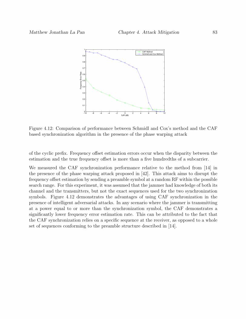
Matthew Jonathan La Pan Chapter 4. Attack Mitigation 83
−10 −8 −6 −4 −2 0 2 4 6 8 100
0.1
0.2
0.3
0.4
0.5
0.6
0.7
0.8
0.9
1
SJR (dB)
Fre
qu
en
cy E
rro
r R
ate
CAF Method
Schmidl and Cox Method
Figure 4.12: Comparison of performance between Schmidl and Cox’s method and the CAFbased synchronization algorithm in the presence of the phase warping attack
of the cyclic prefix. Frequency offset estimation errors occur when the disparity between theestimation and the true frequency offset is more than a five hundredths of a subcarrier.
We measured the CAF synchronization performance relative to the method from [14] inthe presence of the phase warping attack proposed in [42]. This attack aims to disrupt thefrequency offset estimation by sending a preamble symbol at a random RF within the possiblesearch range. For this experiment, it was assumed that the jammer had knowledge of both itschannel and the transmitters, but not the exact sequences used for the two synchronizationsymbols. Figure 4.12 demonstrates the advantages of using CAF synchronization in thepresence of intelligent adversarial attacks. In any scenario where the jammer is transmittingat a power equal to or more than the synchronization symbol, the CAF demonstrates asignificantly lower frequency error estimation rate. This can be attributed to the fact thatthe CAF synchronization relies on a specific sequence at the receiver, as opposed to a wholeset of sequences conforming to the preamble structure described in [14].

Matthew Jonathan La Pan Chapter 4. Attack Mitigation 84
−40 −30 −20 −10 0 10 20 300
0.1
0.2
0.3
0.4
0.5
0.6
0.7
0.8
0.9
1
SJR (dB)
Err
or
Ra
te
Preamble Warping Attack vs. CAF
False Preamble Attack vs. CAF
Preamble Warping Attack vs. S&C
False Preamble Attack vs. S&C
Figure 4.13: Timing estimate error rate as a function of SJR for the CAF synchronizationalgorithm vs. the Schmidl and Cox synchronization algorithm in the presence of variousattacks. The CAF synchronization mitigates the power efficient attacks at the expense ofacquisition complexity.

Chapter 5
Adaptive Dynamic Spectrum AccessRadio Warfare
Looking towards future wireless systems, it is apparent that dynamic spectrum access willbecome an integral technology. This is because current policy has created a kind of fictionaltraffic jam on the radio frequency (RF) spectrum. On one hand it seems like there is noroom for any frequency allocation, which is depicted in Figure 1.1. On the other hand, asignificant portion of the spectrum goes unused depending at different times and frequencies.This phenomenon is illustrated in Figure 5.1 It is becoming clear that DSA technology isboth a pertinent and viable solution to this issue, as described in Section 2.2. With the risein importance of DSA technology, it is critical to investigate DSA interference and electronicwarfare.
As demands on performance of wireless radio frequency networks increase, the availability ofusable spectrum continues to diminish. Spectrum crunch has led to a significant increase inresearch geared towards spectrally efficient technologies. This area of work, coupled with theincreasing flexibility and adaptability afforded to wireless devices by the advent of softwaredefined radio and subsequently cognitive radio, has led to the idea of dynamic spectrumaccess for wireless networks.
Dynamic spectrum access is a broad term which encompasses various types of technology andnetworks. A core principle of all DSA networks, though, is that allocation of spectrum withina licensed frequency band varies in time between different users. A significant amount ofwork has been done to properly define both the term DSA and the different types of networksthat the term refers to [46, 28, 29, 27].
Hierarchical DSA is one approach in particular with a number of advantages as well asa number of questions left to be explored. It is an appealing flavor of DSA because itincorporates licensing and policy–much like that which already exists–with spectrum sensingcognitive radio technology. Summarily, the idea is that ’primary’ users in hierarchical DSA
85

Matthew Jonathan La Pan Chapter 5. Adaptive DSA Radio Warfare 86
Background- Concept of Spectrum hole
The underutilization of spectrum opens up the opportunity toidentify and exploit spectrum holes using OpportunisticSpectrum Access (OSA)Spectrum hole: A band of frequencies assigned to a PU,butat a particular time and specific geographic location, the bandis not being utilized by that user [Haykin 2005].
A promising mechanism to improve the spectrum utilizationby exploiting the spectrum holes is based on theCOGNITIVE RADIO technology.
Institute of Technology, NIRMA University, Gujarat, India Nonparametric Spectrum Sensing in CR 3/24
Figure 5.1: Time-frequency diagram illustrating ’holes’ in the wireless spectrum due toinactivity.
have first rights to the spectrum over a given bandwidth. ’Secondary’ users can then accessspectrum at their discretion as long as they adhere to policies aimed to prevent interferencefor the primary users.
The definitions of users within realistic networks, however, are more nuanced than strictlytwo sets of users, labeled primary and secondary. For example, it is likely desirable for anetwork to place priority on emergency broadcast related transmission, critical military usersor network critical information. In these cases, while it is important to protect the primaryusers of the network, it is critical that these secondary users are not denied service. Thesescenarios give rise to different types of DSA radios, or rather different operating modes.
In the context of a DSA network, it is very useful to consider the problem of radio identifi-cation. In a network where spectrum sharing and coordination is performed autonomously,sensing and policy are not the only factors which impact cognitive radio decisions. In addi-tion, learning over time can help DSA radios better incorporate into the network while stilladhering to the required radio policies. This building of radio ’etiquette’ is critical to DSAnetworks. DSA network security is also a critical issue to consider as it relates to successfulDSA deployment. Behavioral based identification algorithms can help identify and protectnetworks from malignant users and other security threats. Some work has been done inexploring alternative methods [47]. However, the majority of previous work is focused onidentifying and tracking specific radios as opposed to identifying and classifying unknownradios using machine learning methods according to behavior within a DSA network frame-work.
The model used for this study comes from [48], where a radio is operating in a potentiallyhostile environment. The two modes used for this study are abstractions of the ’NIB’ modeand ’Protection’ mode, a useful and practical example of how secondary DSA radios mightbehave according to differing policy. While these modes are the example analyzed in this

Matthew Jonathan La Pan Chapter 5. Adaptive DSA Radio Warfare 87
work, we are hopeful that this work extends easily to many types of DSA radios.
5.1 Hierarchical Dynamic Spectrum Access Networks
Many of the problems involving multi-tiered DSA networks have been studied in detail[48, 49, 26, 50]. This work has given rise to the idea of different operating modes, whichallow networks to assign a different level of priority to secondary user communication. Thedifferences between the radio modes are best understood based on the inherent architectureof a secondary DSA radio.
Hierarchical DSA radios are effectively decision engines with input from a combination ofpolicy based reference knowledge, plus spectrum sensing and observation based information.A simple incarnation of this decision engine can be modeled as a state machine of order 3,as shown in Figure 5.2.
This typical model for a DSA radio is a finite state machine. The scan state is where the radiocombines spectrum sensing knowledge with policy knowledge to make a decision dictatingwhat state it transitions to. The rendezvous state occurs after the radio has chosen a channelor piece of spectrum to transmit on; the radio rescans the RF environment then makes atransition decision. The transmit state represents the radio transmitting and receiving, butfrom the perspective of this model it represents a state where the radio holds until the RFenvironment induces a state change, similar to the scan state.
Scan RF Environment
Available Channels?
Yes
No
Select Channel, Rendezvous
Abandon threshold exceeded?
No
Yes
Transmit
Mode 1
Mode 2
Figure 5.2: Generalized decision engine architecture for a secondary DSA radio. The radioevaluates the RF environment after each transition to determine the next one. The greenand orange arrows show the single difference between the two radio modes’ behaviors. Thestate transition behavior depends only on the current state.

Matthew Jonathan La Pan Chapter 5. Adaptive DSA Radio Warfare 88
The inherent difference between these two radio modes is the channel selection decision. Themode 1 decision engine is based on the policy of minimizing interference to primary users asits primary goal, illustrated in Figure 5.2. The mode 1 radio will not select a channel andbegin to transmit until there is a channel available. This availability is determined based onthe sampled power on a given channel being lower than an occupy threshold σo,f .
A mode 2 radio will go through the same decision flow as the mode 1 radio, with a differentprimary goal. Again referring to Figure 5.2, the mode 2 radio will always select a channel totransmit on, even if the power on every available channel is greater than the occupy thresholdσo,t. This reflects the radio’s primary objective of transmitting its information; minimizinginterference to primary users is a secondary priority. In the event that all channels aredetermined occupied, the mode 2 radio will choose the channel with the lowest measuredpower in order to minimize interference to itself.
.…..
Channels
Pow
er L
evel
Abandon Threshold
Occupy Threshold
Figure 5.3: A visualization of the spectrum sensing information that secondary DSA radiosuse in their decision engine. Channel power measurements, in blue, are taken within thebandwidth of interest and compared to the decision thresholds.
Each radio mode also has a respective abandon threshold, defined as σa,f and σa,t for mode1 and mode 2, respectively. The thresholds are constrained by
σa ≥ σo > 0 (5.1)
for both radio modes. Figure 5.3 is an example of the RF environment with the decisionthresholds imposed to illustrate the secondary radios sensing. These power thresholds de-termine whether a DSA radio will leave a channel that it is occupying to revert to the scanstate. These thresholds may or may not be the same depending on the policies assigned tothe radio modes as well as the RF environment. After abandoning a channel, the secondaryradio reverts to the scan state and loops until it’s objective is achieved.

Matthew Jonathan La Pan Chapter 5. Adaptive DSA Radio Warfare 89
5.2 Traffic Modeling
One of the key factors dictating radio behavior in DSA networks is user traffic. Variablessuch as traffic density, resource availability and average resource usage are important indetermining the behavior of the radios on the network. While radios on non-DSA networksare often modeled statically or piecewise in a stochastic sense, the probability distributionsthat govern DSA radio behavior can change rapidly depending on traffic patterns in a givennetwork. Modeling this behavior starts with modeling the behavior of primary user traffic.
A network with m channels is modeled as an M/M/m queueing system. The arrival of trafficon the network is represented by a continuous random process N(t) with a mean arrival timeof λ. While the expected arrival time is not necessarily fixed, it is reasonable to assume thatit is over the time period of analysis for modeling DSA radio behavior. The service timesfor each arrival are modeled as a continuous random variable ts, with an expected value µ.
We also model the average power of the primary users with the chi-squared distribution
Pprim ∼ σprimχ2(1) (5.2)
where the scale factor σprim represents the average primary user power seen at the secondaryDSA radio. This model is based on the average output of a DSA radio being modeled as aGaussian random variable.
5.3 System Description
RF Observables
SOM Training and Mapping
1
2 N
..…
u(1) u(2) u(L-‐1) u(L) ……
VM VM-‐1 V2 V1 ..…
Wireless Tx
Training/Observation Classification Sequencing
Hidden Markov Model Training and Matching
LLR
Bayesian Decision Engine N-1
Figure 5.4: The high level architecture for the proposed system. The green arrows showthe signal flow for both the training and identification phases of the system. Each differentclass of radio trains against this system in order for an unknown transmitter to be identifiedwithin a known class of radios.
The system model described in this paper can be broken down into three phases. The firststage of the system deals with the classification problem of the RF environment using a

Matthew Jonathan La Pan Chapter 5. Adaptive DSA Radio Warfare 90
self organizing map. The next stage utilizes the classified RF observations for the trainingof Hidden Markov Models that describe each radio. The final stage of the system usesa Bayesian decision metric in order to classify an unknown radio. Figure 5.4 describes thesystem architecture. It is important to note that the system operates in two ways–it has botha training stage and a classification stage which are identical in structure. The motivationfor using a classification scheme for observations of an RF environment stems from the needfor discrete emission HMMs.
5.3.1 Classification with Self Organizing Maps
In order to both classify radio behavior based on a given RF environment, as well as condensethe space of RF observations in a given system, it is helpful to utilize unsupervised learningalgorithms to perform clustering on multidimensional RF observation vectors. We define theobservation vector
Y1(n) =
C(n)p1(n)
...pm(n)
(5.3)
where C ∈ {0, 1, ..,m} is the transmit channel of the secondary radio, where C = 0 representsno transmission. pi ∈ [0,∞) for i ∈ 1, 2, ...,m is the measured power on channel i out ofm channels. Each of the components of the observation vector varies with time, which isdenoted by the discrete index vector n.
In order to utilize this data to train a hidden Markov model, these observations vectors mustbe discretized, meaning that we need a function to perform the mapping
f : Rm+1 → Z. (5.4)
The choice to map the observations to integers is explained in more detail in the next section.In many practical cases the dimensionality of Y1 will be high, as will the entropy of its com-ponents. Subsequently, an ideal solution for this problem incorporates both dimensionalityreduction and efficient quantization of the observation vectors.
A self organizing map (SOM) is an unsupervised learning tool that is well suited to thistask. Self organizing maps are forms of artificial neural networks (ANN) that are trainedvia unsupervised learning to cluster high dimensional data into a discrete two dimensionalspace [51]. This discretization is ideal for converting observations from an RF environmentinto countable emissions suitable for training HMMs.
The self organizing map is initialized with a topology of s× s neurons. The map is trainedusing example vectors via the well known competitive learning algorithm. There are twodifferent training vectors we utilize for this process, defined as
Oi = Yi(n), i = 1, 2 , n = 0, 1, ..., L− 1, L (5.5)
Matthew Jonathan La Pan Chapter 5. Adaptive DSA Radio Warfare 91
where L is the length of the training sequence. This training set is a time series–in n–of datain the observation vector Y .
The second observation vector (i = 2) used to test this system is defined as
Y2(n) =
C(n)||p(n)||1||p(n)||||p(n)||∞s2(p(n))p(n)
, (5.6)
consisting of multiple computed features of the observed RF spectrum. The second, thirdand fourth features, which are norms of the channel power observations, are defined as
||p(n)||l =
(m∑
i=1
pli(n)
)1/l
, (5.7)
where ||p(n)||, the Euclidean norm, is computed for l = 2. In addition, the maximum norm||p(n)||∞ is computed
||p(n)||∞ = max(p1(n), p2(n), ..., pm(n)). (5.8)
The fifth feature, the unbiased sample variance, is defined
s2(p(n)) =1
m− 1
m∑
i=1
(pi(n)− p(n))2 (5.9)
where p(n) is the sample mean of the power observations, also the final feature, defined as
p(n) =1
m
m∑
i=1
pi(n). (5.10)
We chose to use these feature vectors as an alternative basis for classifying the RF observa-tions due to the nature of the SOM classification algorithm. Competitive learning tends tocluster samples that are close in vector space. However, RF observations that are similar arenot necessarily close in vector space. For example, consider two possible observations, oneat time n = n1 where p1, p2, p3 � σo and p4, ..., pm > σa, and another at time n = n2 wherep1, ..., pm−3 > σa and pm−2, pm−1, pm � σa. These scenarios are distant when represented inthe observation vector Y1, however to a DSA radio it represents two similar scenarios wherethere are three channels that seem unoccupied. For these reasons we trained the systemwith multiple observation vectors and compared overall performance in Section 5.4.
For either choice of the observation vector, both the SOM training and mapping will assigneach example vector to a particular node on the s× s map. Formally, the SOM will map
Yi(n)→ ub, n ∈ L, (5.11)

Matthew Jonathan La Pan Chapter 5. Adaptive DSA Radio Warfare 92
for u ∈ Z, specificallyu ∈ {1, 2, .., s2 − 1, s2}. (5.12)
The term u is used as the SOM node index, where ub represents the index of the nodewithin the SOM that is the best match for an observation vector. The map not only groupssimilar observations together, but also develops a unified distance matrix (or a U-matrix)which topologically represents the distance between the nodes in the map. Examples ofthis classification process can be seen in Figures 5.5 and 5.6. The SOM can then outputthe node of each RF observation as a discrete value representing a particular cluster. Thisdiscretization of the observation space facilitates the use of HMMs as the model for the DSAradios.
0 1 2 3 4 5 6 7
0
1
2
3
4
5
6
Mode 1 Observations Neighbor Distance Map
0 1 2 3 4 5 6 7
0
1
2
3
4
5
6
Mode 2 Observations Neighbor Distance Map
Figure 5.5: Neighbor distance maps for the self organizing maps constructed from the RFobservations from each radio mode. These maps are an interpretation of the unified distancematrix that represents the topology of the self organizing map. Black represents the greatestdistances between neurons and yellow represents the least distance.
0 2 4 6 8
0
1
2
3
4
5
6
580 0 475 0 426 0 0 1192
0 0 0 128 0 0 0 3103
112 0 631 0 403 41 428 76
500 0 0 0 146 0 0 105
0 65 28 0 0 0 0 0
56 0 60 15 0 0 43 411
58 301 54 37 25 41 0 60
70 56 0 270 38 0 0 37
Mode 1 Sample Hits on SOM Neurons
0 2 4 6 8
0
1
2
3
4
5
6
632 0 0 132 356 0 3447 0
0 706 0 0 84 0 0 22
61 0 0 0 0 69 52 27
375 191 603 0 55 39 54 46
0 0 0 733 0 0 0 305
127 0 0 0 0 0 0 0
485 0 682 0 0 57 9 74
111 0 0 47 81 58 74 310
Mode 2 Sample Hits on SOM Neurons
Figure 5.6: Sample assignments for each RF observation training vector to the self orga-nizing map. These plots represent the discretization of the observation space via assigningobservation samples to different neurons in the map. The size of the blue hexagon in eachneuron represents the frequency of an observation being assigned to it.

Matthew Jonathan La Pan Chapter 5. Adaptive DSA Radio Warfare 93
5.3.2 Probabilistic Radio Representation Using Hidden MarkovModels
Explicitly modeling DSA radios with different behaviors is a complex problem, especiallyfor an outside observer with limited a priori knowledge of the radio architecture. For thisreason, it is of interest to model these radios stochastically. Since DSA radio behavior isdynamic by definition, it is important to select a model that can preserve and sufficientlyrepresent the transition in radio behavior. Mixture models are a well known method fordescribing similar systems. DSA radios in particular demonstrate state dependent behaviorreminiscent of a Markov chain, shown clearly in Figure 5.2.
We probabilistically represent each of the two radio modes using hidden Markov models.The general underlying state structure of each of these models is described by the transitionmatrix
aij = P [qt = sj|qt−1 = si] 1 ≤ i, j ≤ N (5.13)
where qt is the current observation and qt−1 is the previous, and aij is the transition proba-bility from state i to state j, subject to the constraints
aij ≥ 0 (5.14)
3∑
j=1
aij = 1 (5.15)
In this paper, we would like to consider the more general case aij ∈ RNxN . Since it is feasiblethat the architecture and/or the policy that governs the radio is unknown to the observer, itis important to develop a system for identifying a radio with an unknown number of states.The ergodic state transition model of an unknown radio with N states is
aij =
a0|0 . . . a0|N
.... . .
...aN |0 . . . aN |N
(5.16)
where the notation ai|j represents the state transition probability from i to j.
The emission probability matrices associated with these models are dependent on the methodfor observation quantization used in the HMM training. In order to determine the impact ofthe observation space on the accuracy of radio identification, it is important to compress theinformation from the RF environment to different levels. This idea comes from the unknownunderlying complexity of the DSA radio system. The general emission matrix for the modelis defined
bij = P [vi(t)|qt = sj], 1 ≤ j ≤ N, 1 ≤ i ≤M (5.17)
where v is the set of the discrete positive integer observations and M = |v|. It is important tonote that v ⊂ u and M ≤ s2, meaning not necessarily all of the SOM nodes have observationvectors classified to them during mapping.

Matthew Jonathan La Pan Chapter 5. Adaptive DSA Radio Warfare 94
In this work, the value of M is determined by the number of neurons utilized in SOM training,as shown in Figure 5.6. The discretized training sequences Oi are then used to train hiddenMarkov models for each radio mode via the well known Baum-Welch algorithm. One of themost critical challenges of developing HMMs for these radio modes is the initial guess forthe radio model. We avoided making too many assumptions about the underlying structureof the radios. The models are ergodic, with uniform state transition probabilities, meaning
aij =1
N, 1 ≤ j ≤ N, 1 ≤ i ≤ N. (5.18)
The initialization of the emission probability matrix b is less trivial–the solution at whichthe HMM training algorithm converges is greatly dependent on the initialization of theemission probability matrix [52]. Initializing these probabilities randomly will usually causethe algorithm to converge on a model with uniform state transition probabilities and emissionfrequencies as the output probabilities. This essentially turns the HMM into a one statesystem, which is not the best model, as will be shown in Section 5.4. Instead, we initializethe emission probabilities with random perturbation to a uniform distribution, specifically
bij =1− εj
+ εxij∑
j∈M
xij, 0 ≤ ε ≤ 1. (5.19)
The value of ε is the perturbation factor of the initial distributions, while xij is a set ofstandard uniform independent, identically distributed (i.i.d.) random variables. Any valueof ε > 0 will produce an initial uniform distribution with uniformly distributed perturbations.Once the best guess distributions are determined for the HMMs the models can be trainedand used for classification of unknown radios.
5.3.3 Classifying Unknown Radios
The final stage of the radio identification system classifies unknown radios as either Mode1 or Mode 2. The unknown radio observations are discretized via mapping to trained selforganizing maps. The discrete observation sequences can be used to compute the probabilityP (T |λ) that indicates how likely it is that the sequence came from a HMM described bythe parameter λ. These probabilities are computed using the forward procedure of theBaum-Welch (or forward-backward) algorithm.
Given two radio models, with distinct parameters λ1 and λ2, we can use the log of theprobabilities P (U |λ1) and P (U |λ2) for the unknown observation sequence U to compute thelog likelihood ratio
LLR = log
(P (U |λ1)P (U |λ2)
). (5.20)
The logs of the sequence probabilities are used for computations due to the fact that theactual probabilities can quickly approach zero. The sign of the log likelihood ratio is used

Matthew Jonathan La Pan Chapter 5. Adaptive DSA Radio Warfare 95
to determine the classification of the unknown radio via the Bayesian decision rule, whileLLR’s of zero are classified as undetermined.
5.4 Simulation and Analysis
In order to verify this model and determine it’s performance, we implemented a MATLABsimulation of the two example radio modes, the primary user models and the RF environ-ment. We set the occupy and abandon thresholds for both the federal and tactical moderadios at σo = 10−6 and σa = 10−4. Primary user arrivals were modeled as a homogenousPoisson process, with rate parameter λ = .1 and mean power determined by the randomvariable Pprim where σprim = σa. We modeled a m=10 channel network with exponentialrandom variable service time ts with a mean service time of µ = 1. The channel noise powerPn was assigned a mean value of 10−9. It is important to note that we carefully selected thetraffic parameters to ensure a certain user density within the network. This is an importantaspect of radio identification which greatly impacts the modeling of the radios. In DSAnetworks where secondary radio behavior is guided by policy that protects primary users’ability to access spectrum resources, secondary radio behavior will vary greatly based onprimary user density, as well as overall user density. While investigating the effect of userdensity on this identification system is outside of the scope of this paper, it is an importantpart of our future work.
For HMM training we used variable length training sequences based on traffic from a fixedamount–10,000–users through the channel queue model. Each model was trained on 10 ofthese sequences. In order to simulate a scenario where the number of hidden states for aradio model is unknown, we simulated across a range of states from N = 1 to N = 10.While the model for N = 1 is trivial, it models the radios as having stationary distributions,which can be a simple identification technique if the radio modes demonstrate significantlydifferent emission probabilities. While the initial guess for an unknown system can be greatlyimproved, the problem is not trivial and is a focus for future work.
Table 5.1: Radio Identification Success Rates Using O1, 1 MapNumber of States
s× s 1 2 3 4 5 6 7 8 9 104 .881 .653 .538 1.0 .484 .998 1.0 1.0 1.0 1.09 .958 .897 .806 .775 .991 .949 1.0 .861 .494 1.016 .923 .775 .766 .722 .489 1.0 .52 .999 .162 .88525 .942 .809 .925 .653 .613 1.0 .594 .297 .507 .21536 .948 .905 .939 .516 .564 .494 .731 1.0 .999 .20549 .915 .809 .807 .711 .981 .999 .528 1.0 .156 1.064 .877 .782 .86 .648 .556 1.0 .93 .053 .994 .004
Tables 5.1-5.4 show the simulation results for this work. While there are a number of regions

Matthew Jonathan La Pan Chapter 5. Adaptive DSA Radio Warfare 96
Table 5.2: Radio Identification Success Rates Using O1, 2 MapsNumber of States
s× s 1 2 3 4 5 6 7 8 9 104 .913 .919 .624 .491 .490 1.0 .917 1.0 1.0 1.09 .666 .655 .593 .574 .672 .732 .739 .749 .944 1.016 .974 .840 .819 .645 .656 1.0 1.0 .987 .998 1.025 .469 .469 .469 .469 1.0 .530 .488 1.0 1.0 1.036 .513 .522 .5 .636 .5 .775 1.0 .871 .520 .58049 .523 .520 .526 .596 .523 .621 .657 .714 .957 .99064 .497 .496 .497 .497 .497 .998 .949 .961 .996 1.0
Table 5.3: Radio Identification Success Rates Using O2, 1 MapNumber of States
s× s 1 2 3 4 5 6 7 8 9 104 .878 .897 .498 .869 .474 .995 1.0 1.0 1.0 1.09 .946 0.911 .847 .665 .659 .517 .488 .997 1.0 1.016 .916 .87 .618 .825 .533 1.0 .966 .578 .999 .99425 .872 .882 .676 .526 .614 .52 .88 .98 .508 .44836 .929 .869 .955 .675 .525 .516 .893 .802 .994 .66549 .915 .867 .796 .648 .687 .98 .996 .511 .984 .74864 .886 .846 .803 .611 .93 1.0 .861 .992 1.0 1.0
where the identification system exhibits particularly poor performance–any identificationrate around .5 essentially means the system is just guessing–there are also multiple combina-tions of SOM and HMM size that identify the unknown radios very accurately, in some caseswith perfect accuracy. It is of interest to note that using a SOM size of 4 nodes, which vastlyreduces the entire observation space to 4 discrete outputs, performed perfectly in all caseswhere N > 7. This result is encouraging because simpler implementations of this system aredesirable for realistic implementation.
There seems to be two different regions in each table that demonstrate poor performance.The first is in the lower rows of the Tables 5.2 and 5.4. These regions show particularly lowidentification rates which seem to be attributed to lack of training data. Since two maps areused in these cases, each map is trained with half as much data as in the single map case.Choosing the correct amount of training data for these systems is a focus of further research.The second region demonstrating poor performance lies to the left hand side of each table,where a relatively low number of states is chosen for the HMMs. The last trend shown inthe results is that there are significant drops in performance near many of the areas of peakperformance when looking at the tables in a row-wise fashion. This result indicates thatsystem parameters must be chosen carefully for a practical implementation of this system.Developing the mathematical framework for automatic parameter selection is a key area offuture research.
There were some rather surprising results produced by these simulations as well. There aremultiple cases–such as N=8 and s× s=64 in Table 5.1–where the system trains poorly and

Matthew Jonathan La Pan Chapter 5. Adaptive DSA Radio Warfare 97
Table 5.4: Radio Identification Success Rates Using O2, 2 MapsNumber of States
s× s 1 2 3 4 5 6 7 8 9 104 .923 .902 .6 .469 .469 .976 1.0 1.0 1.0 1.09 .719 .697 .649 .605 .702 .993 .723 1.0 1.0 .93216 .599 .61 .602 .57 .526 .978 1.0 1.0 .948 .56325 .511 .511 .511 .511 .494 .746 .945 1.0 .861 .00236 .518 .518 .518 .518 .518 .657 1.0 .534 1.0 1.049 .597 .583 .569 .561 .486 .869 .982 .947 .997 .98464 .504 .505 .488 .51 .514 .519 .567 .123 .082 .386
identifies the radios almost perfectly incorrectly. In addition, many of the more successfulsimulations of the system occur when N > 5, despite the fact that the underlying decisionengine for the radio modes seem simple. This result may very well be attributed to having noinformation about the initial guesses of the transition and emission matrices for the HMMs,indicating that there is a trade off between a priori knowledge and system complexity. Insome example training for this system, we provided theorized initial guesses to the HMMparameters that we inferred from the behavioral model with much more success for values ofN = 3. Developing better methods for model initialization is a priority for future research.
Chapter 6
Conclusion and Future Work
Physical layer security is an important topic as it relates to 4G and future generations ofsystems. It is important to consider these wireless security issues for a wide scope of systemsand scenarios. As more cognition is introduced in to the realm of electronic warfare, itis critical to find optimal strategies for both attack and defense. In this work we havepresented several strategies and solutions to problems regarding physical layer cognitiveelectronic warfare.
We have discussed how the synchronization process in any system employing OFDM isparamount to successful communications and how this process is also extremely sensitiveto estimation errors [7]. While synchronization methods similar to those proposed in [14]perform very well against uncorrelated interference, the acquisition process can be severelydegraded by intelligent jamming attacks [38, 42]. We have presented a number of these attackstrategies that target the physical layer structure of OFDM synchronization symbols in orderto cripple timing acquisition and carrier frequency offset estimation, along with theoreticaland simulation based performance analysis of OFDM systems in the presence of these attacks.We have also demonstrated how the synchronization performance improves when using CAFsynchronization in the presence of one of these smart jamming attacks. In addition, we haveproposed a structure for securing OFDM synchronization via frame location randomizationof training symbols. These tactics in conjunction with one another offer the possibility ofdramatically improving OFDM synchronization security at the physical layer.
The CAF synchronization methods presented in this paper are a novel approach to perform-ing training based symbol timing acquisition and carrier frequency offset estimation for anOFDM system. We have shown that this method is viable for robustly performing OFDMsynchronization through both mathematical analysis and simulations that incorporate someof the realistic effects of a wireless communication environment. While the methods we pre-sented are relatively costly from a computational standpoint, the algorithms are designed toutilize the efficiency of the DFT, which is inherent to the OFDM structure and lends to lowcost hardware implementation. Furthermore, large portions of the computations can be run
98

Matthew Jonathan La Pan Chapter 6. Conclusion and Future Work 99
in parallel, which increases the feasibility of these algorithms in conjunction with develop-ments in parallel computing technology and the coinciding increase of affordability. Thesemethods, along with future work for synchronization and other vital processing functions,can help to improve the overall security of OFDM based systems.
There are a number of areas for future work in the area of OFDM synchronization securityand ambiguity function based synchronization. It is important to develop a functioningimplementation of the CAF synchronization in order to both demonstrate its viability asprocessing method for OFDM acquisition and carrier frequency offset estimation, but alsoin order to test its performance under realistic multipath conditions and fading scenariosfor the case of mobile OFDM based systems. In addition, the sync-amble randomizationconcept that applies to the OFDM control layer is a concept that can be further developed.This technology would most likely need to make use of a public/private key strategy in orderto grant access to shared information about sync symbol locations.
Looking one layer higher to MAC layer security considerations for future systems, we haveshown that by using a combination of machine learning techniques and probabilistic modelingfor DSA radios that behavior based identification is possible. Cognitive approaches such asthese are vital to developing cognitive radio technology with the ability to deploy in realisticcommunications environments with established infrastructure already in place. The problemof behavior based cognitive radio identification will be fundamental for both commercial andtactical DSA network security research.
By integrating machine learning approaches in to this technique, we have been able to greatlycollapse the space of observations that would typically be available to a DSA radio. Utilizingsequence based stochastic techniques like hidden Markov models in order to model radiospreserves the temporal fidelity of the behavioral statistics. HMMs are shown to be onesuch statistical tool that can provide this type of simplified mathematical representation forcognitive radio decision engine and outputs. We have shown that it is possible to train thissystem and automatically categorize DSA radios based on observable RF behavior with ahigh level of accuracy when model parameters are correctly chosen.
While the initial results are promising and warrant future work on this problem, this area ofwork represents a huge problem space with a plethora of future work. There are still a rangeof variables to consider that will impact the system, including primary user traffic density,observation noise and limitations and improved modeling and initial guesses for DSA radioHMMs. In addition, in order to optimize the system in terms of parameter selection, it willbe important to incorporate some model selection methods based on information theoreticmetrics of the observation space. In addition, there are a number of underlying theoreticalconcepts left to be formalized in order to fully develop this type of system.
The issues of OFDM synchronization and DSA radio security are important to consider forthe future of wireless systems as both technologies become more prevalent. The challengespresented on both the attack and defensive sides of cognitive electronic warfare will only con-tinue to increase in scope and complexity with the development of 4G and future generation

Matthew Jonathan La Pan Chapter 6. Conclusion and Future Work 100
system capabilities. It will be vital for future implementations of OFDM systems to securethe physical layer control processes, particularly synchronization. Likewise, as DSA capabil-ities are realized for wireless systems, developing automated, cognitive algorithms for radiosto assess their environments will be critical to the security of DSA capable networks. It isparamount that adequate wireless physical layer security features are developed to matchthe advances in physical layer technology for modern wireless systems.

Bibliography
[1] H. C. Keong. (2001, November) Overview of OFDM Design. National University ofSingapore.
[2] J. Zhang, Y. Liu, S. Ozdemir, R. Wu, F. Gao, X. Wang, L. Yang, and F. Nori, “Quantuminternet using code division multiple access,” Scientific Reports, vol. 3, 2013.
[3] The IEEE 802.16 Working Group on Broadband Wireless Access Standards, 802.16e-2009, The IEEE 802.16 Working Group on Broadband Wireless Access Standards Std.,2009.
[4] 3rd Generation Partnership Program (3GPP), Long Term Evolution (LTE), The 3rdGeneration Partnership Project (3GPP) Std., 2009.
[5] R. W. Chang, “Synthesis of Band-Limited Signals for Multichannel Data Transmission,”The Bell Systems Technical Journal, vol. 45, pp. 1775–1796, 1966.
[6] S. Weinstein and P. Ebert, “Data Transmission by Frequency-Division MultiplexingUsing the Discrete Fourier Transform,” IEEE Transactions on Communication Tech-nology, vol. 19, pp. 628–634, 1971.
[7] R. van Nee and R. Prasad, OFDM for Wireless Multimedia Communications. Boston,MA: Artech House, 2000.
[8] T. Pollet, M. V. Bladel, and M. Moeneclaey, “BER Sensitivity of OFDM Systems toCarrier Frequency Offset and Wiener Phase Noise,” IEEE Transactions on Communi-cations, vol. 43, no. 2/3/4, Feb/Mar/Apr 1995.
[9] H. Minn, V. Bhargava, and K. Letaief, “A Combined Timing and Frequency Synchro-nization and Channel Estimation for OFDM,” in IEEE International Conference onCommunications (ICC), June 2004.
[10] M. Moretti and I. Cosovic, “OFDM Synchronization in an Uncoordinated SpectrumSharing Scenario,” in IEEE Global Telecommunications Conference (GLOBECOM),November 2007.
101

[11] S. Patil and R. Upadhyay, “A Symbol Timing Synchronization Algorithm for WiMAXOFDM,” in Conference on Computational Intelligence and Communication Networks(CICN), October 2011.
[12] J. Kleider, S. Gifford, G. Maalouli, S. Chuprun, and B. Sadler, “Synchronization forRF Carrier Frequency Hopped OFDM: Analysis and Simulation,” in IEEE MilitaryCommunications Conference (MILCOM), October 2003.
[13] L. Nasraoui, L. Atallah, and M. Siala, “An Efficient Reduced-Complexity Two-StageDifferential Sliding Correlation Approach for OFDM Synchronization in the AWGNChannel,” in IEEE Vehicular Technology Conference (VTC), September 2011.
[14] T. Schmidl and D. Cox, “Robust Frequency and Timing Synchronization for OFDM,”IEEE Transactions on Communications, vol. 45, no. 12, December 1997.
[15] J. Mark and W. Zhuang, Wireless Communications and Networking. Prentice Hall,2003.
[16] P. Schniter, “Low-complexity equalization of OFDM in doubly selective channels,” IEEETransactions on Signal Processing, vol. 52, pp. 1002–1011, 2004.
[17] T. Rappaport, Wireless Communications: Principles and Practice. Prentice Hall, 2002.
[18] T. C. Clancy, “Efficient OFDM Denial: Pilot Jamming and Pilot Nulling,” in IEEEInternational Conference on Communications (ICC), June 2011.
[19] C. Shahriar, S. Sodagari, and T. Clancy, “Performance of pilot jamming on MIMOchannels with imperfect synchronization,” in Communications (ICC), 2012 IEEE In-ternational Conference on, 2012, pp. 898–902.
[20] C. Shahriar, S. Sodagari, R. W. McGwier, and T. C. Clancy, “Performance impactof asynchronous off-tone jamming attacks against OFDM,” in Communications (ICC),2013 IEEE International Conference on, 2013, pp. 2177–2182.
[21] IEEE 802.11af-2013, The IEEE Working Group 802.11- Wireless LAN Working GroupStd.
[22] IEEE 802.22-2011, IEEE 802 LAN/MAN Standards Committee 802.22 WG onWRANs(Wireless Regional Area Networks) Std.
[23] B. Ray, “How to build a national cellular wireless network for 50m,” The Register, April2011.
[24] J. Mitola and G. Q. Maguire, “Cognitive radio: making software radios more personal,”IEEE Personal Communications Magazine, vol. 6, pp. 13–18, 1999.
102

[25] T. C. Clancy, “Dynamic Spectrum Access in Cognitive Radio Networks,” Ph.D. disser-tation, University of Maryland, College Park, 2006.
[26] S. Chan, “Shared Spectrum Access for the DoD,” in New Frontiers in Dynamic SpectrumAccess Networks (DySpan), 2007.
[27] B. Jabbari, R. Pickholtz, and M. Norton, “Dynamic Spectrum Access and Manage-ment,” IEEE Wireless Communications, vol. 17, pp. 6–15, August 2010.
[28] B. S. Qing Zhao, “A Survey of Dynamic Spectrum Access,” IEEE Signal ProcessingMagazine, vol. 24, pp. 78–89, 2007.
[29] M. Sherman, A. Mody, R. Martinez, and C. Rodriguez, “IEEE Standards SupportingCognitive Radio and Networks, Dynamic Spectrum Access, and Coexistence,” IEEEStandards in Communications and Networking, vol. 46, pp. 72–79, 2008.
[30] M. Zilis, “Californias Yurok Tribe Takes Advantage of White Spaces Technology,”Radio Resource Magazine, June 2011.
[31] W. U. Relations, “Nation’s first campus ’Super Wi-Fi’ network launches at West Vir-ginia University,” Press Release, July 2013.
[32] L. Sanguinetti, M. Morelli, and H. V. Poor, “Frame Detection and Timing Acquisitionfor OFDM Transmissions with Unknown Interference,” IEEE Transactions on WirelessCommunications, vol. 9, 2010.
[33] K. Ramiah and M. Zivkovic, “OFDM Synchronization in the Presence of Interference,”in International Conference on Communications, Signal Processing, and their Applica-tions (ICCSPA), 2013.
[34] L. Tao, W. H. Mow, V. K. N. Lau, M. Siu, R. S. Cheng, and R. Murch, “Robust JointInterference Detection and Decoding for OFDM-based Cognitive Radio Systems withUnknown Interference,” IEEE Journals on Selected Areas in Communications, vol. 25,pp. 566–575, 2007.
[35] P. Sun and L. Zhang, “Narrowband Interference Effect on Timing Synchronization forOFDM-based Spectrum Sharing System,” in International Conference on Wireless andMobile Communications (ICWMC), 2010.
[36] M. Marey and H. Steendam, “Analysis of the Narrowband Interference Effect on OFDMTiming Synchronization,” IEEE Transactions on Signal Processing, vol. 55, pp. 4558–4566, 2007.
[37] P. Klenner and K. Kammeyer, “Temporal Autocorrelation Estimation for OFDM withApplication to Spatial Interpolation,” in IEEE Asilomar Conference on Signals, Systemsand Computers, October 2008, pp. 995–999.
103

[38] M. La Pan, T. C. Clancy, and R. W. McGwier, “Jamming Attacks Against OFDMTiming Synchronization and Signal Acquisition,” in IEEE Military CommunicationsConference (MILCOM), October 2012.
[39] P. Moose, “A Technique for Orthogonal Frequency Division Multiplexing frequency off-set correction,” IEEE Transactions on Communication, vol. 42, pp. 2908–2914, October1994.
[40] J. van de Beek, “Low-Complex Frame Synchronization in OFDM Systems,” in Interna-tional Conference on Universal Personal Communications (ICUPC), November 1995,pp. 982–986.
[41] M. Morelli and M. Moretti, “Robust Frequency Synchronization for OFDM-Based Cog-nitive Radio Systems,” IEEE Transactions on Wireless Communications, vol. 7, pp.5346–5355, 2008.
[42] M. La Pan, T. C. Clancy, and R. W. McGwier, “Phase Warping and Differential Scram-bling Attacks Against OFDM Frequency Synchronization,” in International Conferenceon Acoustics Speech and Signal Processing (ICASSP), May 2013.
[43] ——, “Protecting physical layer synchronization: mitigating attacks against OFDMacquisition,” in Wireless Personal Multimedia Communications (WPMC), 2013 16thInternational Symposium on, 2013.
[44] C. Yatrakis, “Computing the Cross Ambiguity Function : A Review,” Master’s thesis,Binghamton University, State University of New York, 2005.
[45] S. Stein, “Algorithms for Ambiguity Function Processing,” IEEE Transactions onAcoustics Speech and Signal Processing, vol. ASSP-29, no. 3, pp. 588–599, June 1981.
[46] IEEE Standard for Spectrum Sensing Interfaces and Data Structures for Dynamic Spec-trum Access and other Advanced Radio Communication Systems., IEEE Std., April2011.
[47] K. Kim, C. Spooner, I. Akbar, and J. Reed, “Specific Emitter Identification for Cogni-tive Radio with Application to IEEE 802.11,” in Gobal Telecommunications Conference(GLOBECOM), November 2008, pp. 1–5.
[48] T. C. Clancy, “Security Recommendations for Military Use of Dynamic Spectrum AccessTechnology,” Office of the Assistant Secretary of Defense for Network and InformationIntegration, Tech. Rep., 2011.
[49] Y. Gottlieb, “Policy-controlled dynamic spectrum access in multitiered mobile net-works,” in Military Communications Conference (MILCOM), 2010.
[50] K. Zhang, D. Swain, and M. Lin, “Dynamic Spectrum Access Enabled DoD Net-centricSpectrum Management,” in Military Communications Conference (MILCOM), 2007.
104

[51] T. Kohonen, “The Self-Organizing Map,” Proceedings of the IEEE, vol. 78, no. 9, pp.1464–1480, September 1990.
[52] L. Rabiner, “A tutorial on hidden Markov models and selected applications in speechrecognition,” Proceedings of the IEEE, vol. 77, pp. 257–286, 1989.
105