Embed Size (px)
Citation preview

MAE 3401 – Modeling and Simulation
SECTION 6: TIME‐DOMAIN ANALYSIS

K. Webb MAE 3401
Natural and Forced Responses2
This first sub‐section of notes continues where the previous section left off, and will explore the difference between the forced and natural responses of a dynamic system.

K. Webb MAE 3401
3
Natural and Forced Responses
In the previous section we used Laplace transforms to determine the response of a system to a step input, given zero initial conditions The driven response
Now, consider the response of the same system to non‐zero initial conditions only The natural response

K. Webb MAE 3401
4
Natural Response
0 (1)
Use the derivative property to Laplace transform (1) Allow for non‐zero initial‐conditions
0 0 0 0 (2)
Same spring/mass/damper system Set the input to zero Second‐order ODE for displacement
of the mass:

K. Webb MAE 3401
5
Natural Response
Solving (2) for gives the Laplace transform of the output due solely to initial conditions
Laplace transform of the natural response
(3)
Consider the under‐damped system with the following initial conditions
1
16
4 ∙
0 0.15
0 0.1

K. Webb MAE 3401
6
Natural Response
Substituting component parameters and initial conditions into (3)
. . (4)
Remember, it’s the roots of the denominator polynomial that dictate the form of the response Real roots – decaying exponentials Complex roots – decaying sinusoids
For the under‐damped case, roots are complex Complete the square Partial fraction expansion has the form
. . ..
(5)

K. Webb MAE 3401
7
Natural Response
. . ..
(5)
Multiply both sides of (5) by the denominator of the left‐hand side
0.15 0.7 2 3.464
Equating coefficients and solving for and gives
0.15, 0.115
The Laplace transform of the natural response:.
.. .
.(6)

K. Webb MAE 3401
8
Natural Response
Inverse Laplace transform is the natural response0.15 cos 3.464 ∙ 0.115 sin 3.464 ∙ (7)
Under‐damped response is the sum of decaying sine and cosine terms

K. Webb MAE 3401
9
Now, Laplace transform, allowing for both non‐zero input and initial conditions
0 0 0
Solving for , gives the Laplace transform of the response to both the input and the initial conditions
(8)
Driven Response with Non‐Zero I.C.’s
1

K. Webb MAE 3401
10
Laplace transform of the response has two components
Total response is a superposition of the initial condition response and the driven response
Both have the same denominator polynomial Same roots, same type of response
Over‐, under‐, critically‐damped
Driven Response with Non‐Zero I.C.’s
Natural response ‐ initial conditions Driven response ‐ input

K. Webb MAE 3401
11
Driven Response with Non‐Zero I.C.’s
Laplace transform of the total response
0.15 0.7 10.15 0.7 1
Transform back to time domain via partial fraction expansion
22 3.464
3.4642 3.464
Solving for the residues gives
0.0625, 0.0875, 0.0794
1
16
4 ∙
0 0.15
0 0.1
1 ∙ 1

K. Webb MAE 3401
12
Driven Response with Non‐Zero I.C.’s
Total response:0.0625 0.0875 cos 3.464 ∙ 0.0794 sin 3.464 ∙
Superposition of two components Natural responsedue to initial conditions
Driven response due to the input

K. Webb MAE 3401
Next, we’ll apply the Laplace transform to the entire state‐space model in matrix form, just as we did for single differential equations.
Solving the State‐Space Model13

K. Webb MAE 3401
14
Solving the State‐Space Model
We’ve seen how to use the Laplace transform to solve individual differential equations
Now, we’ll apply the Laplace transform to the full state‐space system model
First, we’ll look at the same simple example Later, we’ll take a more generalized approach
State‐space model is
10
10
(1)0 1
Note that, because this model was derived from a bond graph model, the state variables are now momentum and displacement

K. Webb MAE 3401
15
Laplace Transform of the State‐Space Model
For now, focus on the state equation Output is a linear combination of states and inputs Determining the state trajectory is the important thing
Use the derivative property to Laplace transform the state equation
00 0
10
Rearranging to put all transformed state vectors on the left‐hand side
000
10 (2)

K. Webb MAE 3401
16
Laplace Transform of the State‐Space Model
000
10 (2)
Can factor out the transformed state vector from the left‐hand side Must multiply by a 2 2 identity matrix
000
10
00 0
00
10
00
10 (3)

K. Webb MAE 3401
17
Laplace Transform of the State‐Space Model
00
10 (3)
Note the form of (3) The LHS is , where is the system matrix Everything on the RHS reduces to a vector A known matrix times a vector of unknowns equals a known vector
If we can solve for and/or , we can inverse transform to get and/or Use Cramer’s Rule
K. Webb MAE 3401
18
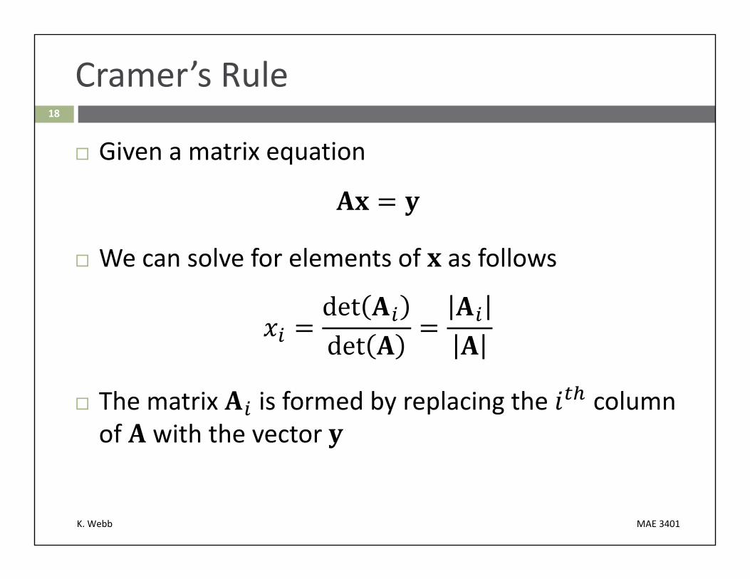
Cramer’s Rule
Given a matrix equation
We can solve for elements of as follows
The matrix is formed by replacing the column of with the vector

K. Webb MAE 3401
19
Laplace Transform of the State‐Space Model
According to Cramer’s Rule
(4)
According to the output equation from (1)
Equation (4) is identical to (8) from the previous subsection of notes, which we arrived at differently

K. Webb MAE 3401
20
Laplace Transform of the State‐Space Model
(5)
Next, sub in parameter values, I.C.’s and an input Use PFE to inverse transform to Again, consider the under‐damped system:
Let the input be a step:
1
16
4 ∙
0 0.15
0 0.1 ∙

K. Webb MAE 3401
21
Laplace Transform of the State‐Space Model
The Laplace transform of the output becomes. . .
. . (6)
Inverse transform via partial fraction expansion. . .
.(7)
Multiply both sides by left‐hand‐side denominator0.15 0.7 1 4 16 2 3.464
Equating coefficients and solving yields
0.0625, 0.0875, 0.0794

K. Webb MAE 3401
22
Laplace Transform of the State‐Space Model
The Laplace transform of the system response is. .
.. .
.(8)
The time‐domain response is0.0625 0.0875 cos 3.464 0.0794 sin 3.464 (9)
Transient portion Due to initial conditions
and input step Decays to zero
Steady‐State portion Due to constant input Does not decay

K. Webb MAE 3401
23
Laplace Transform of the State‐Space Model
Now, we’ll apply the Laplace transform to the solution of the state‐space model in general form
For now, focus on the state equation only Output is derived from states and inputs
Laplace transform of the state equation
0
Rearranging
0
Factoring out the transformed state from the left‐hand side
0 (10)

K. Webb MAE 3401
24
Laplace Transform of the State‐Space Model
0 (10)
Remember the dimensions of each term in (10) : : 1 : 1
: 1 0 : 1
Apply Cramer’s rule to solve for the Laplace transform of the state variable
(11)
The matrix is formed by replacing the column of with 0
An 1 vector of known values

K. Webb MAE 3401
25
Laplace Transform of the State‐Space Model
(11)
Denominator of (11) is the determinant of is an matrix
Each diagonal term is a first‐order polynomial in One term in the determinant is the trace of the matrix, the product terms along
the diagonal is an ‐order polynomial in
The characteristic polynomial:
Δ (12)
Roots of Δ are values of that satisfy the characteristic equation
Δ 0 (13) Poles of (11) Eigenvalues of system matrix,

K. Webb MAE 3401
26
Laplace Transform of the State‐Space Model
Denominator of every state variable’s Laplace transform contains the characteristic polynomial
(14)
A characteristic of the system Remember, denominator roots (i.e. poles) determine the nature of
the response Real roots – decaying exponentials Complex roots – decaying sinusoids
Responses of all state variables have same components Numerators of transforms determine the differences
Output transform has the same denominator, Δ Linear combination of states and input Response includes the same sinusoidal and/or exponential components

K. Webb MAE 3401
27
Laplace Transform of the State‐Space Model
Assume: zero initial conditions: 0 SISO system: single input – is a scalar transform
Can factor out the input from the numerator of (14)
∗
where ∗ is the matrix formed by replacing the column of with the vector
appears in every term of one column of appears in every term of the determinant
K. Webb MAE 3401
28
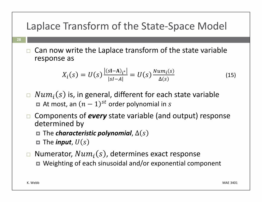
Laplace Transform of the State‐Space Model
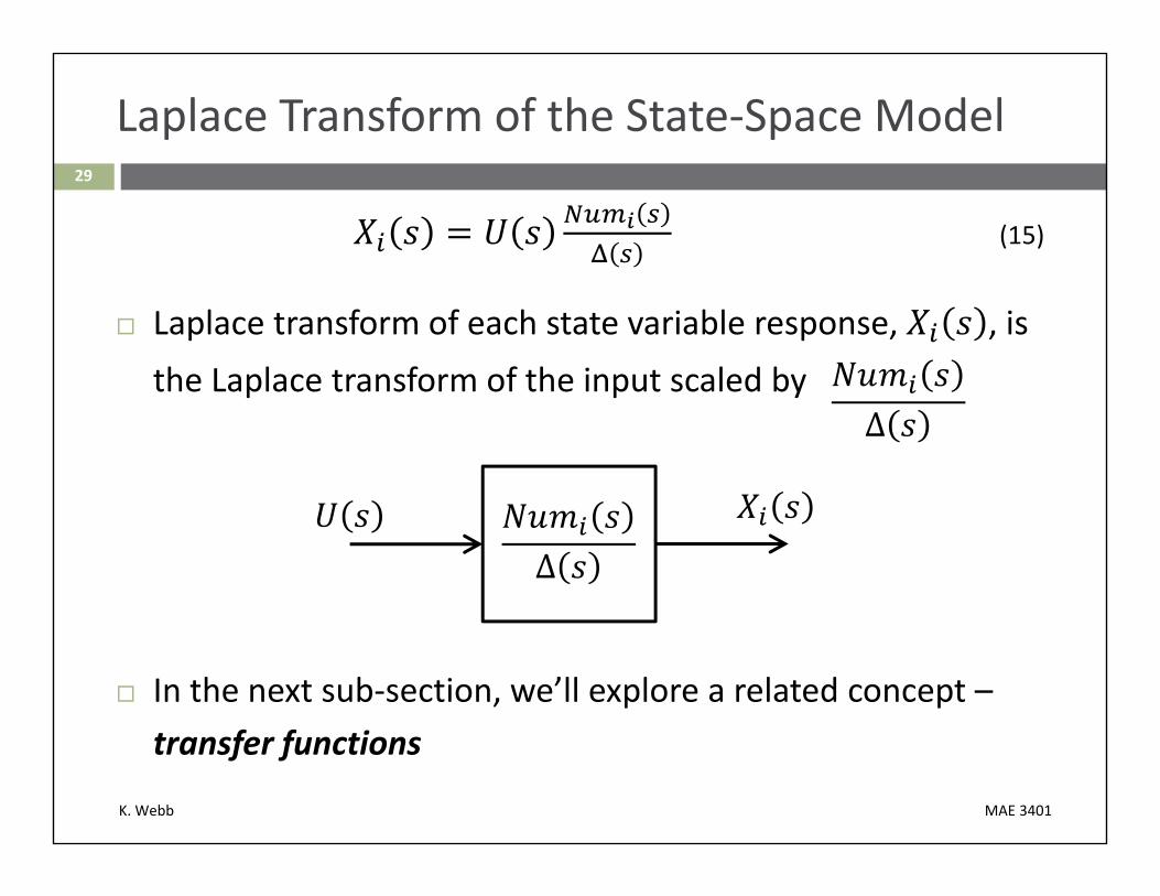
Can now write the Laplace transform of the state variable response as
∗(15)
is, in general, different for each state variable At most, an 1 order polynomial in
Components of every state variable (and output) response determined by The characteristic polynomial, Δ The input,
Numerator, , determines exact response Weighting of each sinusoidal and/or exponential component
K. Webb MAE 3401
29
Laplace Transform of the State‐Space Model
(15)
Laplace transform of each state variable response, , is the Laplace transform of the input scaled by
Δ
In the next sub‐section, we’ll explore a related concept –transfer functions
Δ

K. Webb MAE 3401
Transfer Functions30

K. Webb MAE 3401
31
Transfer Functions
Now, come back to the full state‐space model, including the output equation – (SISO case assumed here ‐ and are scalars)
D
Assume zero initial conditions and Laplace transform the whole model
(1)
D (2)
Simplify the state equation as before
Solving for the state vector
(3)

K. Webb MAE 3401
32
Transfer Functions
Substituting (3) into (2) gives the Laplace transform of the output
D
Factoring out the inputD (4)
Transform of the output is the input scaled by the stuff in the square brackets
Dividing through by the input gives the transfer function
D (5)
Ratio of system’s output to input in the Laplace domain, assuming zero initial conditions
An alternative to the state‐space (time‐domain) model for mathematically representing a system

K. Webb MAE 3401
33
Transfer Matrix – MIMO Systems
For MIMO systems
inputs: is 1, is outputs: is 1, is
Transfer function becomes a matrix
Transfer function relates the output to the input
We’ll continue to assume SISO systems in this course

K. Webb MAE 3401
34
Transfer Functions
System output in the Laplace domain is the input multiplied by the transfer function
We saw earlier that state variables are given by
where is the characteristic polynomial
Output is linear combination of states and input, so we’d expect the denominator of to be as well Is it? What is the denominator of ?

K. Webb MAE 3401
35
Transfer Functions
D (5)
The matrix inverse term in (5) is given by
where the numerator is the adjoint of Equation (5) can be rewritten as
(6)
Transfer function denominator is the characteristic polynomial Poles of the transfer function are roots of Δ
System poles or eigenvalues Eigenvalues of the system matrix, Along with the input, system poles determine the nature of the time‐domain
response

K. Webb MAE 3401
This sub‐section of notes takes a bit of a tangent to explain the use of the term eigenvalues when referring to system poles.
Eigenvalues36

K. Webb MAE 3401
37
Eigenvalues
We’ve been using the term eigenvalue when referring to system poles – why? Recall from linear algebra, the eigenvalue problem
(1)
where: is an matrixis an 1 vector – an eigenvectoris a scalar – an eigenvalue
Eigenvalue problem involves finding both the eigenvalues and the eigenvectorsthat satisfy (1)
Eigenvalues and eigenvectors are specific to (characteristics of) the matrix An matrix will have, at most, eigenvalues and corresponding eigenvectors
Equation (1) says: An 1 eigenvector, , left‐multiplied by an matrix, , results in an 1 vector The resulting vector is the eigenvector scaled by the eigenvalue, Result is in the same direction as – i.e., not rotated

K. Webb MAE 3401
38
Eigenvalues and Eigenvectors
Geometrically, multiplication of a vector by a matrix results in two things Scaling and rotation
Consider the matrix
1 34 2
And the vectors
11 , 1
0 Compute the product
In both cases, results have different magnitudes and different directions

K. Webb MAE 3401
39
Eigenvalues and Eigenvectors
Multiplication of a matrix and one of its eigenvectors results in scaling only No rotation
The 2 2matrix1 34 2
has two eigenvectors (normalized)
0.7070.707 and 0.6
0.8and two corresponding eigenvalues
λ 2 and λ 5
such that
and

K. Webb MAE 3401
40
Eigenvalues and Eigenvectors
A full‐rank, matrix will have pairs of eigenvalues and eigenvectors
To find all eigenvalues and eigenvectors that satisfy (1)
(1)rearrange
and factor out the eigenvector term
0 (2)
If exists, then , which is the trivial solution and of no interest
We’re interested in values of and that satisfy (2) when is not invertible – when it is singular

K. Webb MAE 3401
41
Eigenvalues and Eigenvectors
Want to find values of for which is singular A matrix is singular if its determinant is zero
0 (3)
Equation (3) is the characteristic equation for is the characteristic polynomial, Δ An ‐order polynomial in
Eigenvalues of matrix are all values of that satisfy (3) Roots of the characteristic polynomial Find the corresponding eigenvectors by substituting into (2) and solving for
Letting , (3) becomes the denominator of the system transfer function,

K. Webb MAE 3401
Using the Transfer Function to Determine System Response42

K. Webb MAE 3401
43
Using to determine System Response
System output in the Laplace domain can be expressed in terms of the transfer function as
(1)
Laplace‐domain output is the product of the Laplace‐domain input and the transfer function
Response to two specific types of inputs often used to characterize dynamic systems Impulse response Step response
We’ll use the approach of (1) to determine these responses

K. Webb MAE 3401
44
Impulse response
Impulse function
0, 0
1
Laplace transform of the impulse function is
1
Impulse response in the Laplace domain is
1 ∙
The transfer function is the Laplace transform of the impulse response Impulse response in the time domain is the inverse transform of the
transfer function
K. Webb MAE 3401
45
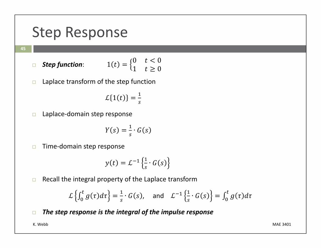
Step Response
Step function: 1 0 01 0
Laplace transform of the step function
1
Laplace‐domain step response
∙
Time‐domain step response
∙
Recall the integral property of the Laplace transform
∙ , and ∙
The step response is the integral of the impulse response

K. Webb MAE 3401
46
First‐ and Second‐Order Systems
All transfer functions can be decomposed into 1st‐ and 2nd‐order terms by factoring Δ Real poles – 1st‐order terms Complex‐conjugate poles – 2nd‐order terms
These terms and, therefore, the poles determine the nature of the time‐domain response Real poles – decaying exponentials Complex‐conjugate poles ‐ decaying sinusoids
All time‐domain responses will be a superposition of decaying exponentials and decaying sinusoids These are the natural modes or eigenmodes of the system
Instructive to examine the responses of 1st‐ and 2nd‐order systems Gain insight into relationships between pole location and response

K. Webb MAE 3401
Response of First‐Order Systems47
K. Webb MAE 3401
48
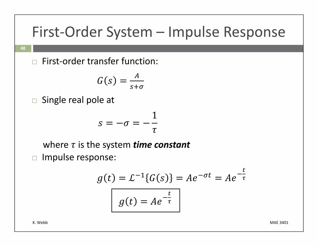
First‐Order System – Impulse Response
First‐order transfer function:
Single real pole at 1
where is the system time constant Impulse response:

K. Webb MAE 3401
49
First‐Order System – Impulse Response
Initial slope is inversely proportional to time constant
Response completes 63% of transition after one time constant
Decays to zero as long as the pole is negative

K. Webb MAE 3401
50
Impulse Response vs. Pole Location
Increasing corresponds to decreasing and a faster response

K. Webb MAE 3401
51
First‐Order System – Step Response Step response in the Laplace domain
∙
Inverse transform back to time domain via partial fraction expansion
: →
: 0 →
/ /
Time‐domain step response

K. Webb MAE 3401
52
First‐Order System – Step Response
Initial slope is inversely proportional to time constant
Response completes 63% of transition after one time constant
Almost completely settled after 7

K. Webb MAE 3401
53
Step Response vs. Pole Location
Increasing corresponds to decreasing and a faster response

K. Webb MAE 3401
54
Pole Location and Stability
First‐order transfer function
where is the system pole Impulse response is
If 0, decays to zero Pole in the left half‐plane System is stable
If 0, grows without bound Pole in the right half‐plane System is unstable

K. Webb MAE 3401
Response of Second‐Order Systems55

K. Webb MAE 3401
56
Second‐Order Systems
Second‐order transfer function
(1)
where is the damped natural frequency
Can also express the 2nd‐order transfer function as
(2)
where is the un‐damped natural frequency, and is the damping ratio
1
Two poles at
, 1

K. Webb MAE 3401
57
Categories of Second‐Order Systems
The 2nd‐order system poles are
, 1
Value of determines the nature of the poles and, therefore, the response
: Over‐damped Two distinct, real poles – sum of decaying exponentials – treat as two first‐order terms ,
: Critically‐damped Two identical, real poles – time‐scaled decaying exponentials ,
: Under‐damped Complex‐conjugate pair of poles – sum of decaying sinusoids , 1
: Un‐damped Purely‐imaginary, conjugate pair of poles – sum of non‐decaying sinusoids ,

K. Webb MAE 3401
58
2nd‐Order Pole Locations and Damping

K. Webb MAE 3401
59
Second‐Order Poles ‐
Can relate , , , and to pole location geometry
is the magnitude of the poles is a measure of system
damping
sin
0 Two purely imaginary poles
1 Two identical real poles
1 Two distinct real poles

K. Webb MAE 3401
60
Impulse Response – Critically‐Damped
For , the transfer function reduces to
2
Impulse response

K. Webb MAE 3401
61
Impulse Response – Critically‐Damped
Speed of response is proportional to

K. Webb MAE 3401
62
Impulse Response – Under‐Damped
For 0 1, the transfer function is
2
Complete the square on the denominator
1
Rewrite in the form of a damped sinusoid
Inverse Laplace transform for the time‐domain impulse response
sin

K. Webb MAE 3401
63
Under‐Damped Impulse Response vs.
sin sin 1

K. Webb MAE 3401
64
Under‐Damped Impulse Response vs.
sin sin 1

K. Webb MAE 3401
65
Impulse Response – Un‐Damped
For 0, the transfer function reduces to
Putting into the form of a sinusoid
Inverse transform to get the time‐domain impulse response
An un‐damped sinusoid
sin

K. Webb MAE 3401
66
Un‐Damped Impulse Response vs.
sin

K. Webb MAE 3401
67
Second‐Order Step Response
The Laplace transform of the step response is1
The time‐domain step response for each damping case can be derived as the the inverse transform of
or as the integral of the corresponding impulse response

K. Webb MAE 3401
68
Critically‐Damped Step Response vs.
11

K. Webb MAE 3401
69
Under‐Damped Step Response vs.
11 cos sin

K. Webb MAE 3401
70
Under‐Damped Step Response vs.
11 cos sin

K. Webb MAE 3401
71
Un‐Damped Step Response vs.
11 cos

K. Webb MAE 3401
2nd‐Order Step Response Characteristics72

K. Webb MAE 3401
73
Step Response – Risetime
Risetime is the time it takes a signal to transition between two set levels Typically 10% to 90% of full transition
Sometimes 20% to 80%
A measure of the speed of a response
Very rough approximation:
.

K. Webb MAE 3401
74
Step Response – Overshoot
Overshoot is the magnitude of a signal’s excursion beyond its final value Expressed as a percentage of full‐scale swing
Overshoot increases as decreases
%OS
0.45 20
0.5 16
0.6 10
0.7 5

K. Webb MAE 3401
75
Step Response –Settling Time
Settling time is the time it takes a signal to settle, finally, to within some percentage of its final value Typically 1% or 5%
Inversely proportional to the real part of the poles,
For 1% settling:
. .

K. Webb MAE 3401
In this sub‐section, we’ll see that the time‐domain output of a system is given by the convolution of its time‐domain input and its impulse response.
The Convolution Integral76

K. Webb MAE 3401
77
Convolution Integral
Laplace transform of a system output is given by the product of the transform of the input signal and the transfer function
∙
Recall that multiplication in the Laplace domain corresponds to convolution in the time domain
∗
Time‐domain output given by the convolution of the input signal and the impulse response
∗

K. Webb MAE 3401
78
Convolution
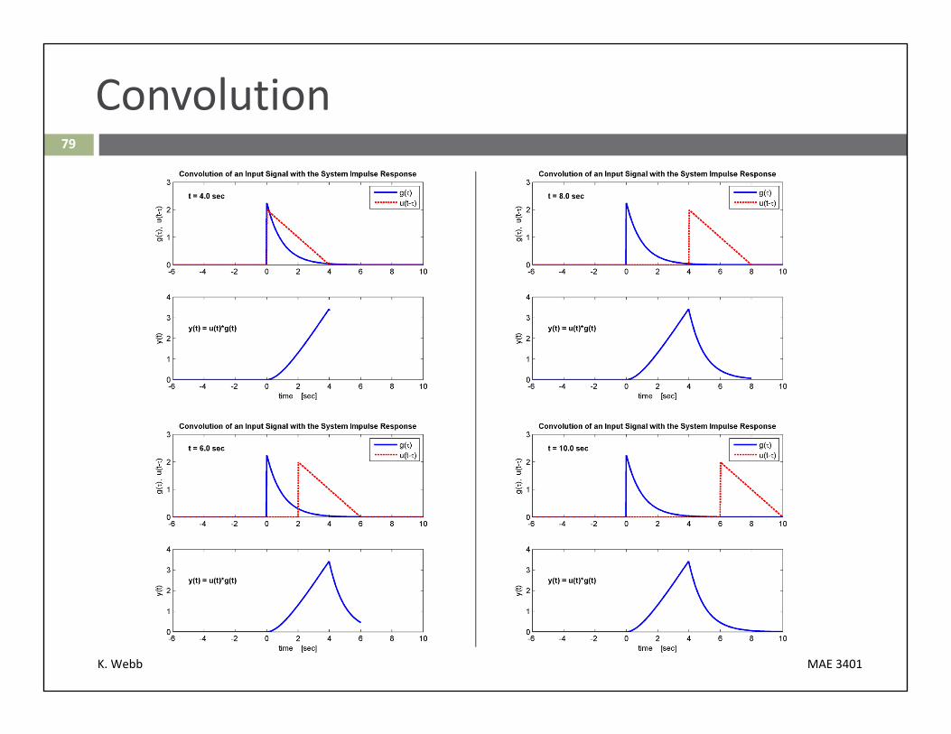
Time‐domain output is the input convolved with the impulse response
∗
Impulse response is flipped in time and shifted by
Multiply input and flipped/shifted
Integrate over 0…
Each time point of given by result of integral with
shifted by
K. Webb MAE 3401
79
Convolution

K. Webb MAE 3401
80
Convolution

K. Webb MAE 3401
A few of MATLAB’s many built‐in functions that are useful for simulating linear systems are listed in the following sub‐section.
Time‐Domain Analysis in MATLAB81

K. Webb MAE 3401
82
System Objects
MATLAB has data types dedicated to linear system models
Two primary system model objects: State‐space model Transfer function model
Objects created by calling MATLAB functions ss.m – creates a state‐space model tf.m – creates a transfer function model
K. Webb MAE 3401
83
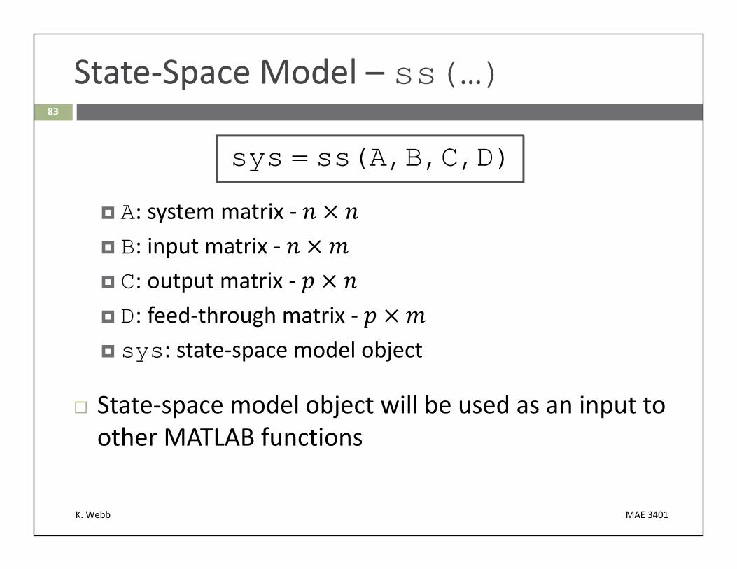
State‐Space Model – ss(…)
sys = ss(A,B,C,D)
A: system matrix ‐ B: input matrix ‐ C: output matrix ‐ D: feed‐through matrix ‐ sys: state‐space model object
State‐space model object will be used as an input to other MATLAB functions
K. Webb MAE 3401
84
Transfer Function Model – tf(…)
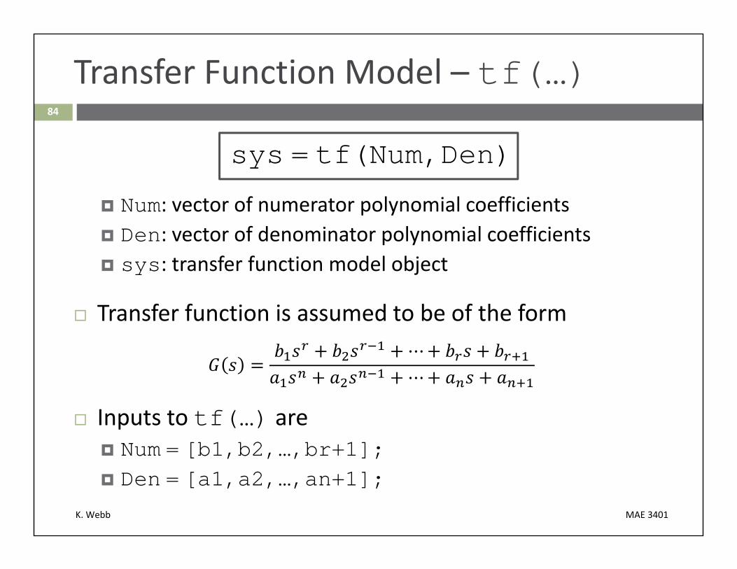
sys = tf(Num,Den)
Num: vector of numerator polynomial coefficients Den: vector of denominator polynomial coefficients sys: transfer function model object
Transfer function is assumed to be of the form⋯⋯
Inputs to tf(…) are Num = [b1,b2,…,br+1]; Den = [a1,a2,…,an+1];

K. Webb MAE 3401
85
Step Response Simulation – step(…)
[y,t] = step(sys,t)
sys: system model – state‐space or transfer function t: optional time vector or final time value y: output step response t: output time vector
If no outputs are specified, step response is automatically plotted
Time vector (or final value) input is optional If not specified, MATLAB will generate automatically

K. Webb MAE 3401
86
Impulse Response Simulation – impulse(…)
[y,t] = impulse(sys,t)
sys: system model – state‐space or transfer function t: optional time vector or final time value y: output impulse response t: output time vector
If no outputs are specified, impulse response is automatically plotted
Time vector (or final value) input is optional If not specified, MATLAB will generate automatically
K. Webb MAE 3401
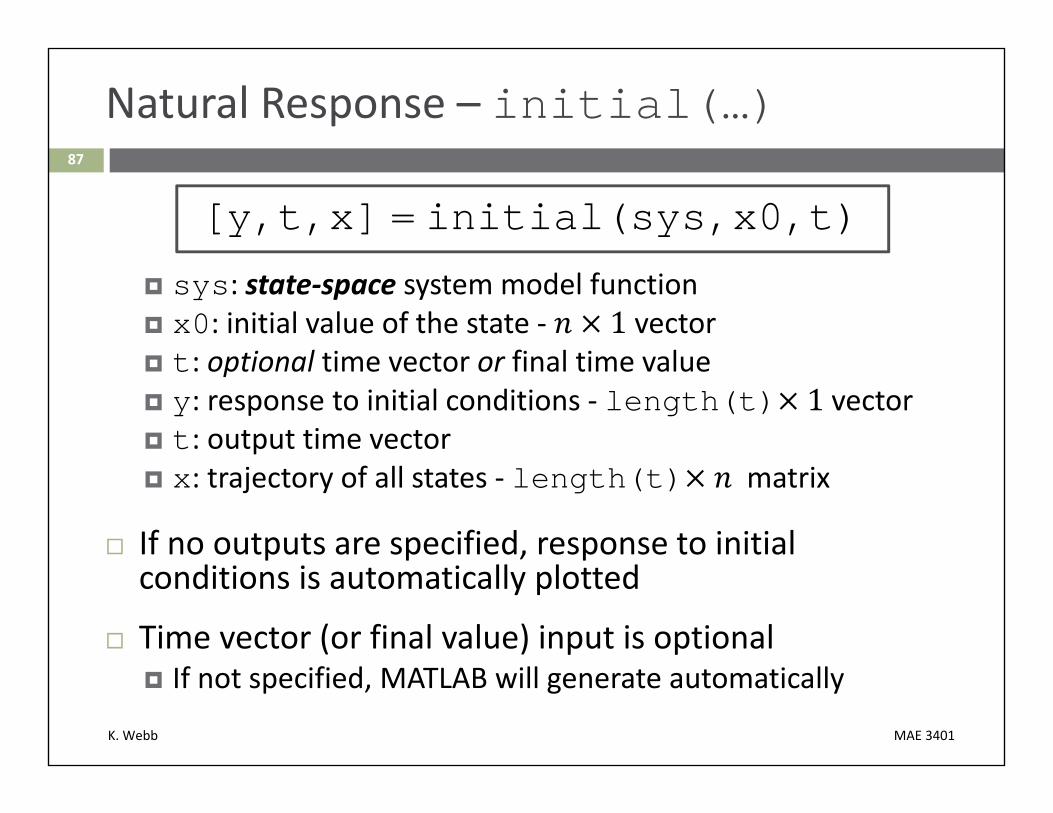
87
Natural Response – initial(…)
[y,t,x] = initial(sys,x0,t)
sys: state‐space system model function x0: initial value of the state ‐ 1 vector t: optional time vector or final time value y: response to initial conditions ‐ length(t) 1 vector t: output time vector x: trajectory of all states ‐ length(t) matrix
If no outputs are specified, response to initial conditions is automatically plotted
Time vector (or final value) input is optional If not specified, MATLAB will generate automatically

K. Webb MAE 3401
88
Linear System Simulation – lsim(…)
[y,t,x] = lsim(sys,u,t,x0)
sys: system model – state‐space or transfer function u: input signal vector t: time vector corresponding to the input signal x0: optional initial conditions – (for ss model only) y: output response t: output time vector x: optional trajectory of all states – (for ss model only)
If no outputs are specified, response is automatically plotted
Input can be any arbitrary signal

K. Webb MAE 3401
89
More MATLAB Functions
A few more useful MATLAB functions
Pole/zero analysis: pzmap(…) pole(…) zero(…) eig(…)
Input signal generation: gensig(…)
Refer to MATLAB help documentation for more information