Seasonal weather patterns drive population vital rates and …sites.warnercnr.colostate.edu/kanno/wp-content/uploads/sites/112/2… · (Salvelinus fontinalis) at a broad spatial scale

Seasonal weather patterns drive population vital ratesand persistence in a stream fishYO ICH IRO KANNO1 , BEN JAMIN H . LETCHER 2 , NATHANIEL P . H I TT 3 ,

DAV ID A . BOUGHTON4 , JOHN E . B . WOFFORD 5 and ELISE F. ZIPKIN6

1Department of Forestry and Environmental Conservation, Clemson University, 261 Lehotsky Hall, Clemson, SC 29634, USA,2Silvio O. Conte Anadromous Fish Research Branch, Leetown Science Center, United States Geological Survey, One Migratory Way,

Turners Falls, MA 01376, USA, 3Leetown Science Center, United States Geological Survey, 11649 Leetown Road, Kearneysville,

WV 25430, USA, 4Fisheries Ecology Division, Southwest Fisheries Science Center, National Oceanic and Atmospheric

Administration, 110 Shaffer Road, Santa Cruz, CA 95060, USA, 5Shenandoah National Park, 3655 Hwy 211 East, Luray, VA

22835, USA, 6Department of Integrative Biology, Michigan State University, 288 Farm Lane, East Lansing, MI 48824, USA

Abstract

Climate change affects seasonal weather patterns, but little is known about the relative importance of seasonal

weather patterns on animal population vital rates. Even when such information exists, data are typically only avail-

able from intensive fieldwork (e.g., mark–recapture studies) at a limited spatial extent. Here, we investigated effects

of seasonal air temperature and precipitation (fall, winter, and spring) on survival and recruitment of brook trout

(Salvelinus fontinalis) at a broad spatial scale using a novel stage-structured population model. The data were a 15-year

record of brook trout abundance from 72 sites distributed across a 170-km-long mountain range in Shenandoah

National Park, Virginia, USA. Population vital rates responded differently to weather and site-specific conditions.

Specifically, young-of-year survival was most strongly affected by spring temperature, adult survival by elevation

and per-capita recruitment by winter precipitation. Low fall precipitation and high winter precipitation, the latter of

which is predicted to increase under climate change for the study region, had the strongest negative effects on trout

populations. Simulations show that trout abundance could be greatly reduced under constant high winter precipita-

tion, consistent with the expected effects of gravel-scouring flows on eggs and newly hatched individuals. However,

high-elevation sites would be less vulnerable to local extinction because they supported higher adult survival. Fur-

thermore, the majority of brook trout populations are projected to persist if high winter precipitation occurs only

intermittently (≤3 of 5 years) due to density-dependent recruitment. Variable drivers of vital rates should be com-

monly found in animal populations characterized by ontogenetic changes in habitat, and such stage-structured effects

may increase population persistence to changing climate by not affecting all life stages simultaneously. Yet, our

results also demonstrate that weather patterns during seemingly less consequential seasons (e.g., winter precipita-

tion) can have major impacts on animal population dynamics.

Keywords: air temperature, climate change, count data, N-mixture models, precipitation, salmonids, stage-structured

populations

Received 28 April 2014 and accepted 24 October 2014

Introduction

Climate change can shift species ranges and affect ani-

mal abundance via alterations in local weather condi-

tions (Thomas et al., 2004; Chen et al., 2011). While

understanding these biological patterns is important

for conservation planning and adaptive management,

few studies have investigated the demographic pro-

cesses that bring about population-scale changes (e.g.,

Wright et al., 2009; Hegel et al., 2010; Nilsson et al.,

2011; Vindenes et al., 2014). Although climate change

affects weather patterns during all seasons, the relative

importance of different seasons on population vital

rates has rarely been investigated (Dybala et al., 2013),

with a vast majority of studies focused on either a sin-

gle season or annual weather variables (e.g., Hunter

et al., 2010; Roland & Matter, 2013; Wenger et al., 2013).

Yet, animal populations respond to seasonal weather

variations in complex and unexpected ways for a num-

ber of reasons.

First, many life history strategies are tightly linked to

seasonality, and a consistent change in a weather pat-

tern (e.g., temperature increase) can differentially affect

vital rates during different seasons (Wright et al., 2009;

Fern�andez-Chac�on et al., 2011; Diamond et al., 2013;

Dybala et al., 2013). Second, animal populations are

structured by age, size or life stage, and individualsCorrespondence: Yoichiro Kanno, tel. 864-656-1645,

fax: 864-656-3304, e-mail: [email protected]

1856 © 2014 John Wiley & Sons Ltd

Global Change Biology (2015) 21, 1856–1870, doi: 10.1111/gcb.12837

require different resources through ontogeny (Werner

& Gilliam, 1984). Different individuals are unlikely to

respond uniformly to a specific climatic condition, with

potentially large differences among life stages (Haslob

et al., 2012; Diamond et al., 2013; Dybala et al., 2013).

Finally, animal populations are additionally regulated

by density-dependent factors, and population density

has been shown to influence recruitment and survival

across many taxa (Nicola et al., 2008; Diamond et al.,

2013; Lok et al., 2013). The magnitude of density depen-

dence can affect population stability and resiliency

(Lack, 1954) under changing weather conditions.

Robust inferences on the effect of weather patterns on

population vital rates require long-term data sets with

rich demographic information. Accordingly, the small

number of previous studies that have examined this

issue relied primarily on intensively collected field data

from a single population or a limited number of popula-

tions (e.g., Letcher et al., 2007; Wright et al., 2009; Dybal-

a et al., 2013). Mark–recapture methods are commonly

employed to estimate vital rates in intensive field stud-

ies conducted at relatively small spatial scales (Williams

et al., 2002). However, population vital rates can differ

greatly among populations distributed along environ-

mental gradients (Jenouvrier et al., 2009; Fern�andez-

Chac�on et al., 2011; Lobøn-Cervi�a, 2014; Roth et al.,

2014), suggesting that the impact of climate drivers var-

ies not only temporally but also spatially. Current

anthropogenic threats to biodiversity, such as climate

change and land use, operate at broad spatial scales. We

need a fuller understanding of how spatial heterogene-

ity and seasonal weather affect population vital rates to

identify the environmental origins of population vul-

nerability. This means that long-term data sets must be

spatially replicated for robust inferences about effects

of seasonal weather on vital rates. Mark–recapturemethods cannot easily provide such replication because

they are expensive and labor intensive.

Obtaining animal count data without mark–recapturemethods is less labor intensive and allows researchers

to collect data at broader spatial and temporal scales.

Count data have been used less frequently than mark–recapture data in demographic analyses of animal pop-

ulations (e.g., Gross et al., 2002; Link et al., 2003; Alonso

et al., 2011) because the lack of individual histories in

count data is assumed to limit inference about vital

rates. Recent advances in the analysis of count data pro-

vide a promising approach to breaching this limit. Dail

& Madsen (2011) proposed a statistical approach that

modeled apparent survival and recruitment rates based

on count data distributed over space and time. The

method was further extended by Zipkin et al. (2014a)

who demonstrated that demographic heterogeneity

among individuals (e.g., age, size, and sex) can be esti-

mated with this framework. This structured population

model provides a flexible method for incorporating

temporal and spatial heterogeneity in the environment

as well as density-dependent processes into the

analysis of count data, but its applications to empirical

data have been limited to date (Kanno et al., 2014;

Zipkin et al., 2014b).

In this study, we use a structured population model

to investigate effects of mean air temperature and pre-

cipitation during fall, winter, and spring seasons on the

survival and recruitment of brook trout (Salvelinus fonti-

nalis). We drew on a 15-year count record collected

from 72 sites distributed across a 170-km-long moun-

tain range in Shenandoah National Park (SNP), Vir-

ginia, USA. Air temperature and precipitation are

drivers of stream temperature and flow, which in turn

are considered the key physical drivers of population

dynamics in lotic ecosystems (Poff et al., 1997; Arismen-

di et al., 2013). Numerous studies have shown that

stream fish populations respond to average and

extreme states of these drivers (e.g., Roghair et al., 2002;

Perry & Bond, 2009; Xu et al., 2010a). Yet, the relative

influence of seasonal weather patterns and spatial het-

erogeneity on population vital rates of aquatic species

is unknown across broad spatial scales. Stream temper-

ature and flow are both expected to respond to climate

change via alterations in air temperature and precipita-

tion regimes (Novotny & Stefan, 2007; Huntington

et al., 2009). Consequently, there is a critical need for

understanding how air temperature and precipitation

affect the population dynamics of stream fish, particu-

larly for southern populations of coldwater species

such as brook trout for which climate change is of great

concern. This is challenging because stream fish tend to

be cryptic, elusive, and small bodied, such that individ-

ual detection is imperfect. To be useful, methods for

inferring vital rates from count data must account for

this imperfect detection.

We had two specific objectives. The first was to

develop a stage-structured population model to quan-

tify the effects of seasonal mean maximum air tempera-

ture and precipitation on vital rates, while accounting

for density dependence in recruitment and environ-

mental variation across stages and sampling locations.

The majority of previous stream fish studies have

focused on the effects of summer conditions on popula-

tion vital rates (Boss & Richardson, 2002; Xu et al.,

2010a), and there exists a critical knowledge gap during

other seasons (e.g., Jensen & Johnsen, 1999; Carlson

et al., 2008; Berger & Gresswell, 2009). Our second

objective was to use the stage-structured model for

assessing potential responses of brook trout popula-

tions to climate change using climate projections for the

study region. Our interest lies in determining whether

© 2014 John Wiley & Sons Ltd, Global Change Biology, 21, 1856–1870

SEASONAL WEATHER PATTERNS AND FISH VITAL RATES 1857

certain seasonal weather conditions were more impor-

tant than others to population persistence and how the

frequencies of adverse seasonal weather would affect

population persistence.

Materials and methods

Study species

Brook trout are native to eastern North America, ranging from

Georgia, USA to Labrador and Quebec, Canada. They inhabit

clear and coldwaters. Stream temperature and flow are major

factors that determine population dynamics of brook trout. A

stream temperature range of 21–22°C causes physiological

stress (Hartman & Cox, 2008; Warren et al., 2012) and affect

distribution and abundance of wild populations (McKenna &

Johnson, 2011). Reduced stream flow has been shown to

decrease survival during summer in headwater streams (Xu

et al., 2010a), and floods have been related to short-term popu-

lation declines (Roghair et al., 2002).

Brook trout populations have declined greatly due to a

combination of anthropogenic activities, particularly in the

southern portion of their range where they currently occur

only in high-elevation streams along the Appalachian Moun-

tains (Hudy et al., 2008). Brook trout in headwater streams are

typically short-lived (<3–4 years old) (Grossman et al., 2010;

Xu et al., 2010b; Kanno et al., 2012), and most body growth

takes place during spring months (March–June) in streams

located in the northern USA range (Xu et al., 2010b). Brook

trout spawn during fall, and females excavate small depres-

sions in gravel substrates called ‘redds’ in which fertilized

eggs develop until hatching in late winter to early spring.

Microhabitat preferences change through ontogeny. Young-

of-year (YOY) individuals (<1 year old) are more common at

shallower depths, while older trout prefer deeper and slower

sections of streams such as pools (Kanno et al., 2012; Anglin &

Grossman, 2013). The ontogenetic habitat shifts in brook trout

suggest that the same environmental factors probably affect

adults and YOY individuals differently. For example, Xu et al.

(2010a) reported that in headwater streams in Massachusetts,

summer drought reduced the survival of large brook trout

(>135 mm fork length) but not of smaller individuals. In high-

elevation streams in West Virginia, a winter flood decreased

YOY abundance more severely than adult abundance because

trout redds were scoured during the flood (Carline & McCul-

lough, 2003). However, the generality of these stage-specific

impacts of seasonal weather is not known.

Fish data

We used long-term monitoring data collected by the National

Park Service (NPS) between 1996 and 2010 at 72 sites distrib-

uted across a 170-km-long mountain range in the SNP, Vir-

ginia, USA (Fig. 1). The study area lies within the Blue Ridge

physiographic region characterized by steep slopes and nar-

row ridges. Elevation of the study sites ranged from 285 to

802 m (median = 436 m), and this constitutes important

changes in aquatic habitats and fish assemblages. Sites were

located on small headwater streams (first to third order) that

were well shaded by riparian vegetation and were generally

characterized as step-pool or cascade habitats (Table 1).

Stream flow typically peaked in spring due to snowmelt, fol-

lowed by low-flow conditions in late summer to fall. Study

sites typically harbor few fish species. The most common spe-

cies other than brook trout were blacknose dace (Rhinichthys

Fig. 1 Map of the Shenandoah National Park (shaded by green) showing fish survey sites (brown circles). Streams are shown in blue

lines.


1858 Y. KANNO et al.

atratulus), mottled sculpin (Cottus bairdi), and fantail darter

(Etheostoma flabellare) (Jastram et al., 2013).

At each site, NPS personnel conducted surveys by first

establishing a 100-m stream section by walking within the

stream channel with a metered tape. Upstream and down-

stream ends of sites were typically bounded by natural geo-

morphic habitat breaks that impeded fish movement (e.g.,

step pools). Where geomorphic breaks were inadequate to

impede movement across site boundaries, cobble dams or

block nets were temporarily set up for the survey. Brook trout

were surveyed between May and August (mostly June to

August). The NPS has maintained a brook trout population

monitoring program since 1982 (Jastram et al., 2013), and we

used a portion of this long-term data set collected during

1996–2010. This corresponded with a period during which the

sampling protocol emphasized visiting the same sites repeat-

edly across years to the extent possible. The number of yearly

surveys ranges from 3 to 15 among sites (mean = 7 surveys

per site). Two sites were surveyed annually during the 15-year

study period. Of the total potential sampling occasions (72

sites 9 15 years = 1080 occasions), data were available on 611

occasions (57%).

Backpack electro-shockers were used to sample fish. In

most sampling occasions (81% or 514 of 611 occasions), three-

pass depletion surveys were conducted to infer individual

detection probabilities. In the remaining occasions, single-pass

electrofishing was conducted. We assumed fish populations

were closed to movement during surveys because site bound-

aries coincided with natural geomorphic breaks, cobble dams

or block nets. The number of electrofishing backpack units

used ranged between 1 and 3 depending on stream width.

Each electrofisher was accompanied by two dip netters. Sam-

pling crews proceeded upstream by sampling all available

habitats. Captured fish were measured for total length

(�1 mm) and mass (�0.1 g) and returned to the stream after

all passes were completed. YOY individuals can be distin-

guished from older individuals (‘adults’ hereafter) based on

length–frequency distributions (Xu et al., 2010b; Kanno et al.,

2014). A length–frequency histogram was plotted for each site

9 year combination, and the cutoff size between the two

stages was determined individually (see Appendix S1 for

example histograms). This generated fish count data by site,

year, stage, and sampling replicate (electrofishing pass).

Temperature and precipitation data

We characterized mean seasonal maximum air temperature

and total precipitation at each site in each year. Seasons were

defined as fall (September–November), winter (December–February) and spring (March–May). Summer temperature and

precipitation were not characterized because fish surveys were

primarily conducted during summer months. Thus, the defini-

tion of summer period would have differed among sites and

years, which made interpretation of results challenging. We

did not consider that the omission of summer would weaken

our analysis greatly because summer is by far the most com-

monly studied season in population biology of brook trout

and other freshwater fish. For example, high summer temper-

ature and drought conditions have been associated with popu-

lation declines of brook trout (Hakala & Hartman, 2004;

Table 1 Summary of seasonal and site-specific environmental data in the Shenandoah National Park, Virginia, USA, between 1996

and 2010

Median Mean Min. Max.

Seasonal weather*

Fall precipitation (mm) 363.3 347.3 117.0 566.9

Winter precipitation (mm) 208.7 245.0 95.2 515.7

Spring precipitation (mm) 316.6 311.1 199.7 420.8

Fall temperature (°C) 18.1 18.3 16.6 20.0

Winter temperature (°C) 6.8 6.4 2.9 9.2

Spring temperature (°C) 17.3 17.2 15.0 19.5

Local sites†Latitude 38°47280N 38°49450N 38°09700N 38°82610NLongitude 78°46820W 78°39160W 78°81180W 78°15430WElevation (m) 458 436 285 802

Channel slope (%) 7 5 1 21

Catchment area (km2) 9.3 7.6 1.3 36.2

Wetted stream width (m) 5.9 5.5 3.4 10.8

Water depth (m) 0.34 0.33 0.23 0.54

*Seasonal weather data were based on the Daymet database (http://daymet.ornl.gov). Seasonal precipitation represents total

amount of precipitation in each season, and seasonal temperature represents mean daily maximum air temperature in each season.

For each year, seasonal precipitation and temperature values were calculated by averaging across 72 study sites. Summary statistics

shown above are median, mean and range across the 15-year study period.

†Elevation, channel slope and catchment area were derived in GIS from the National Elevation Dataset (http://ned.usgs.gov/).

Wetted stream width and water depth were based on measurements in the field at ten transects located perpendicular to stream

flow and spaced equally across the upstream–downstream length.



http://daymet.ornl.gov

http://ned.usgs.gov/

Xu et al., 2010a; Warren et al., 2012). However, relative

importance of other seasons on population dynamics is little

known for freshwater fish and is the main focus of our study.

Air temperature and precipitation data at the study sites

were derived from the Daymet database (http://day-

met.ornl.gov). The Daymet model generates daily maximum

and minimum air temperature values at the resolution of

1 km2. We used daily maximum air temperature values to cal-

culate seasonal mean maximum air temperature for each year

at each site (hereafter ‘seasonal air temperature’). Precipitation

represented total amount of precipitation estimated by

Daymet in each season at each site (hereafter ‘seasonal precipi-

tation’). Winter precipitation includes a mix of snow and

rain, although snowfall is commonly recorded during early

spring (March and April) and late fall (November) in the

study area.

Statistical analysis

We examined the effects of seasonal air temperature and pre-

cipitation on population vital rates using a stage-structured

open population N-mixture model (Zipkin et al., 2014a). Clas-

sic N-mixture models estimate population abundance at a set

of local sites over a time period during which the population

is assumed to be closed to births/deaths and immigration/

emigration (Royle, 2004). Abundance is inferred by employing

a repeated sampling scheme that estimates the detection prob-

ability of individuals. Dail & Madsen (2011) extended N-mix-

ture models to open populations where population size can

change over time due to a survival process and a ‘gains’ pro-

cess (recruitment and immigration) in which all individuals

contribute equally to population growth. Their approach has

been further extended for more realistic situations in which

individual heterogeneity, as represented by age, size or sex, is

explicitly accounted for (Zipkin et al., 2014a).

Our model uses a stage-structured population framework

to provide inferences on abundance and population vital rates

in relation to environmental covariates. We assumed an

annual population model of brook trout in the SNP comprised

of two stages: YOY and adults (Fig. 2). A portion of YOY indi-

viduals survive annually and transition into the adult stage

within sites. Surviving adults remain in the same adult stage

in the following year. YOY and adults typically survive at dif-

ferent annual probabilities (Petty et al., 2005; Letcher et al.,

2007), and survival was modeled for each stage. We assumed

that only adults were capable of reproducing offspring. While

size- and age-at-maturity information does not exist in the

SNP brook trout populations, brook trout mature at 100 mm

total length in other populations (Hudy et al., 2010; Kanno

et al., 2011a) and this body length corresponded well with our

YOY–adult cutoff body length in most sites and years (Appen-

dix S1). We assumed that population dynamics were indepen-

dent across sites. We did not explicitly model immigration

and emigration based on the assumption of no net dispersal in

and out of a local site. This is a plausible assumption because

each site was generally established at a representative section

of a stream.

We defined our count data, yi,t,j,k, as the observed count of

individuals at site i in year t for stage j and electrofishing pass

k. Count data (yi,t,j,k) represent a portion of true annual abun-

dance (Ni,t,j) of stage j at site i in year t, due to imperfect detec-

tion. Our main interest was to infer annual vital rates that

governed the spatial and temporal variation in Ni,t,j and to elu-

cidate how these vital rates were affected by environmental

covariates. Our approach allowed for establishing a link

between annual population dynamics and weather patterns in

preceding seasons, as used in other studies (e.g., Diamond

et al., 2013; Heisler et al., 2014). Below, we describe our model

structure, followed by our model selection approach in rela-

tion to the effect of environmental covariates on vital rates.

The population abundance for YOY (j = 1) and adults

(j = 2) in the first year of sampling was assumed to follow a

Poisson distribution such that Ni,1,j ~ Poisson(ki,j) for all sam-

pling sites {i = 1,. . .,72} and stages {j = 1,2}, where ki,j is the

mean abundance of stage j individuals at site i in the first year

of sampling. We modeled ki,j as a function of elevation to

account for potential variation in abundance among sites:

logðki;jÞ� a0j þ a1j � elevationi

where a0j represents the intercept and a1j represents the effect

of elevation on the abundance of stage j individuals.

In subsequent years (t ≥ 2), abundance (Ni,t,j) was modeled

according to the survival and recruitment processes. We

assumed that the annual number of surviving individuals fol-

lowed a binomial process (with parameter xi,t,j), where total

adult abundance was a sum of surviving individuals from

both YOY (j = 1) and adult (j = 2) stages:

Ni;t;2 ¼ BinomialðNi;t�1;1;xi;t;1Þ þ BinomialðNi;t�1;2;xi;t;2Þ:Survival probabilities, xi,t,j, were modeled for each stage j

as a function of seasonal air temperature and precipitation as

well as local elevation using the logit link:

logitðxi;t;jÞ ¼ b0j þ Bj � Xi;t

where b0j is the intercept and the Bj vector represents regres-

sion weights (effect size) for covariates Xi,t (i.e., fall tempera-

ture, winter temperature, spring temperature, fall

precipitation, winter precipitation, spring precipitation, and

elevation) for stage j in site i at year t (but local elevation does

not change among years and does not need indexing by year).

Fig. 2 Annual life cycle of brook trout populations represented

by young-of-year (YOY) and adult stages. Vital rates are

denoted by xi,t,1 (YOY survival probability), xi,t,2 (adult survival

probability), and ci,t (per-capita recruitment rate) for site i in

year t to indicate that these vital rates were estimated for each

site, year, and stage.





Each of the seasonal weather covariates was standardized to

have a site-specific mean of zero and a standard deviation of

one, and elevation was standardized to have a mean of zero

and a standard deviation of one.

We similarly modeled recruitment according to a Markov-

ian process by assuming that local YOY abundance (Ni,t,1) was

a Poisson random variable and depended on adult abundance

in the previous year (Ni,t-1,2):

Ni;t;1 �Poissonðci;t �Ni;t�1;2Þ:The parameter ci,t is the per-capita recruitment probability

in site i and year t. We again model ci,t using the seasonal

weather covariates and elevation. In addition, we included a

density-dependent spawner–recruit function, the Ricker

model (Maceina & Pereira, 2007). The Ricker model has fre-

quently been used to describe spawner–recruit relationships

in salmonid populations for which spawning habitats are a

limiting factor (e.g., Richards et al., 2004; Nicola et al., 2008).

Brook trout females are known to spawn over and thus dis-

rupt existing redds (i.e., redd superimposition) (Essington

et al., 1998), establishing a mechanism for density dependence

at this stage. Spawning habitat is typically limited (Blanchfield

& Ridgway, 2005), suggesting that density dependence is

more likely to occur at this transition than during subsequent

survival. In fact, recruit abundance declined at high spawner

abundance in the SNP brook trout populations (see Appendix

S2). Accordingly, we modeled ci,t by combining the density-

independent (environmental covariates) and density-depen-

dent terms by following Hilborn & Walters (1992):

logðci;tÞ ¼ c0� c1 �Ni;t;2 þ C � Xi;t

where c0 is the productivity coefficient (per-capita recruitment

rate at low spawner abundance), c1 is the density-dependent

coefficient, and C represents the effects of each environmental

covariate represented by Xi,t. Note that c0 is only interpretable

as the productivity coefficient if each covariate in vector X has

been centered such that its mean = 0. We note that we had

also fit another common density-dependent spawner–recruitfunction, the Beverton–Holt model. However, the Ricker

model fits our data set better than the Beverton–Holt model.

For example, the Deviance information criteria (DIC) value of

the final model reported in this article was 43 567 (Ricker

model) vs. 61 438 (Beverton–Holt model).

Modeling detection probabilities

Individual detection probabilities were estimated from the

three-pass depletion data by assuming that the number of

individuals subject to detection decreases in successive elec-

trofishing passes. The observed count of individuals at site i in

year t for stage j and electrofishing pass k, denoted yi,t,j,k, was

modeled by assuming that detection probabilities (pi,t,j) were

constant across passes but could vary by stage and sampling

occasion:

yi;t;j;1 �BinomialðNi;t;j; pi;t;jÞ

yi;t;j;2 �BinomialðNi;t;j � yi;t;j;1; pi;t;jÞ

yi;t;j;3 �BinomialðNi;t;j � yi;t;j;1 � yi;t;j;2; pi;t;jÞ:The models above included two covariates that are surro-

gates of stream flow, which is known to affect electrofishing

sampling efficiency, or pi,t,j (Falke et al., 2010; McCargo & Pet-

erson, 2010). Stream flow data were not available in our study

sites, and we thus used Julian date and stream width as surro-

gates for stream flow. Julian date was used to approximate the

temporal pattern of decreasing stream flow (i.e., higher elec-

trofishing efficiency) from the beginning of the sampling sea-

son (May) to the end (August) observed in the SNP region

during 1996–2010 (see Appendix S3 for summer stream dis-

charge patterns). In addition, body growth of YOY during this

period can lead to increasing capture rates. Mean stream wet-

ted width represents variation in stream size among sampling

locations and was calculated from field measurements taken

perpendicular to flow at every 10 m along the sample site on

the day that fish sampling occurred. Accordingly, detection

probabilities were modeled:

logitðpi;t;jÞ ¼ d0j þ d1 � ðJulian datei;tÞ þ d2 � ðwetted widthi;tÞ

where d0j is the intercept, and d1 and d2 are the effects of the

two covariates at site i in year t. The intercept term is stage

specific because electrofishing is size selective (Reynolds &

Kolz, 2012). Both Julian date and wetted width were standard-

ized to have a mean of zero and a standard deviation of one.

Selection of covariates

The stage-structured model described thus far can include all

environmental variables (i.e., fall temperature, winter temper-

ature, spring temperature, fall precipitation, winter precipita-

tion, spring precipitation, and elevation) as covariates for each

survival and recruitment submodel. However, we only used a

subset of these covariates in our estimates of survivorship and

recruitment to improve parsimony and facilitate ecological

interpretation.

Covariate selection involved the following steps. First, we

examined correlation of all pairs of seasonal weather covari-

ates. Fall temperature and precipitation were significantly cor-

related (Pearson’s r = �0.70), while all other pairs were not

highly correlated (|Pearson’s r| < 0.50). Thus, we ran a model

omitting fall temperature in all submodels and another omit-

ting fall precipitation and then compared the effect size of fall

temperature vs. precipitation. For each submodel, we selected

the fall weather covariate with a larger effect size in absolute

magnitude. This approach allowed us to retain different fall

weather covariates for the survival and recruitment processes.

Second, we ran a new model using the selected fall weather

covariate for each submodel and diagnosed the model output

by examining the posterior correlation of parameters. When

high posterior correlation was observed between a pair of esti-

mated covariate slopes (|Pearson’s r| > 0.5), only the covari-

ate with a larger effect size was retained. Finally, we

evaluated the importance of covariates by their estimated

coefficient size. Covariates whose 95% credible interval (95%

CI) overlapped 0 were dropped from the model. We used DIC



values to confirm model improvement (Spiegelhalter et al.,

2002).

Analysis of the models

We analyzed our models with a Bayesian approach using

Markov chain Monte Carlo (MCMC) methods in JAGS (Plum-

mer, 2003) called from Program R (R Development Core

Team, 2013) with the rjags package (Plummer, 2011) (see

Appendix S4 for JAGS code). We used Jeffery’s priors

(mean = 0 and SD = 1.643) for the effect size of survival and

detection covariates (uninformative on the logit scale). Inter-

cept terms of survival and detection probabilities were slightly

truncated (unif (0.1, 0.9)) based on prior beliefs about the

likely range of sampling efficiency and to facilitate model con-

vergence. Posterior distributions of model parameters were

estimated by taking every 10th sample from 10 000 iterations

of three chains after discarding 10 000 burn-in iterations.

Model convergence was checked by visually examining plots

of the MCMC chains for good mixture as well as with the R-

hat statistic. This statistic compares variance within and

between chains, and models are considered to have converged

when the value is less than 1.1 for all model parameters (Gel-

man & Hill, 2007).

As a measure of model goodness of fit, we plotted predicted

vs. observed fish count for each stage and electrofishing pass

using the selected model. We calculated the proportion of pre-

dicted values that were above observed values (Gelman,

2003). A perfect model would have a value of 0.5 for this

goodness-of-fit statistic, with values closer to zero and one

indicative of poor model fit (Gelman, 2003; K�ery & Schaub,

2012).

Demographic analysis

Using mean survivorship and recruitment estimates, we ran

elasticity analyses to examine the effect of a proportional

change in each vital rate on overall population growth rate,

while holding covariates (mean air temperature and precipita-

tion, and elevation) at their mean values. We used three values

of local adult abundance in the elasticity analysis (for the den-

sity-dependent recruitment portion). These values corre-

sponded to low local abundance (10 individuals per 100 m:

10th percentile of estimated local abundance when pooled

over sites and years), median (45 individuals per 100 m: 50th

percentile), and high abundance (121 individuals per 100 m:

90th percentile). We calculated the population growth rate

and its elasticity to YOY survival, adult survival, and per-cap-

ita recruitment rate at each level of local abundance using the

‘popbio’ package (Stubben & Milligan, 2007) in Program R.

Scenario simulations

To explore model behavior and the potential effects of cli-

mate change (alterations in seasonal air temperature and

precipitation), we simulated two sets of future environmen-

tal scenarios over 30 years (twice the length of the study

period). The first set of scenarios assumed temporally

constant seasonal weather. To do this, we defined ‘high’

and ‘low’ conditions as �1.5 standard deviations (SD) from

the mean value of each seasonal covariate (i.e., fall tempera-

ture, winter temperature, spring temperature, fall precipita-

tion, winter precipitation, and spring precipitation),

corresponding to uncommon events that occurred in an

average of once per 15 years in the historical climate (the

study period). We projected mean annual brook trout abun-

dances in our study sites for 12 simulations (six covariates

9 two conditions) in which the high or low condition for a

seasonal covariate persisted for 30 years after the end of

our 15-year study period, while the other environmental

conditions were held constant at their mean values.

The second set of scenarios represented different frequen-

cies of high winter precipitation. High winter precipitation,

along with low fall precipitation, impacted population abun-

dance most negatively (see Results). Winter precipitation is

predicted to increase under climate change for the region: In a

recent review paper, Ingram et al. (2013) summarized that pre-

cipitation is projected to increase in the study region for all

seasons except summer. Forecasts of precipitation are typi-

cally more uncertain than those of air temperature. Even so, a

15% increase in winter precipitation has been predicted for the

study region for the period 2041–2070 relative to the period

1971–2000 (Ingram et al., 2013). We changed the frequencies of

high winter precipitation (historical mean +1.5*SD) to under-

stand how brook trout populations may respond and how

these responses might differ among locations. Four winter

precipitation scenarios were considered over the course of

30 years (after the 15-year data period); (i) high winter precipi-

tation occurs once every five years, while the mean winter pre-

cipitation condition occurs in other years; (ii) high winter

precipitation occurs in three consecutive years, followed by

two winters with the mean precipitation condition; (iii) high

winter precipitation occurs in four consecutive years, followed

by one winter with the mean precipitation condition; and (iv)

high winter precipitation occurs every year (i.e., identical to

the setting in the first set of simulations earlier). In all four sce-

narios, other seasonal covariates were held to their mean val-

ues. For each of the second set of simulations, we recorded the

number of local sites that experienced ‘quasi-extinction’,

defined here as a local site which had ≤5 individuals for each

of the two stages (YOY and adult) at the end of the simulation

period (i.e., the 45th year).

Results

The selected population model included fall and spring

temperature for YOY survival, and fall, winter, and

spring precipitation, and elevation for adult survival

(Table 2). The recruitment submodel included fall and

winter precipitation, and winter and spring tempera-

ture, and elevation (Table 2). The R-hat values were

less than 1.04 for all parameters in the model. There

was a good concordance between predicated and

observed trout count for each stage and electrofishing

pass, with the goodness-of-fit statistic ranging between

0.36 and 0.76. Model selection details are provided in



Appendix S5, and diagnostics are summarized in

Appendix S6.

Detection probabilities and abundance

Adult detection probability [mean = 0.64, 95% credible

interval (CI) = (0.63–0.64)] was higher than YOY detec-

tion probability [mean = 0.50, 95% CI = (0.49, 0.51)]

(Table 2). Julian date had a significantly positive effect

on detection probability [mean = 0.17, 95% CI = (0.15,

0.19)] (Table 2), suggesting that detection probability

increased from May to August. Stream width had a sig-

nificant negative effect [mean = �0.17, 95%

CI = (�0.19, �0.15)], suggesting that trout capture was

more difficult in wider streams.

Annual total abundance estimates summed across 72

sites was generally lower for adults (mean = 4071 indi-

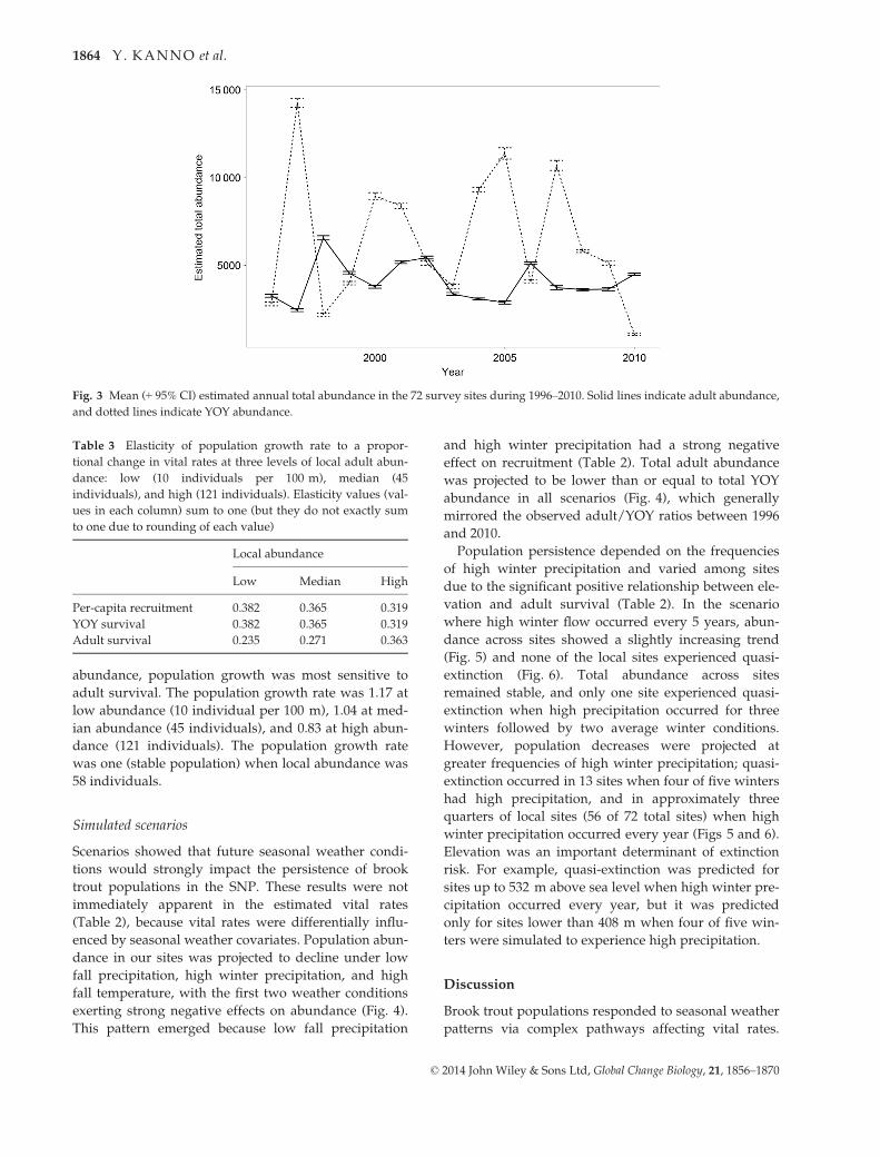
viduals) than YOY (mean = 6461) (Fig. 3). YOY abun-

dance fluctuated more widely over time than adult

abundance: Coefficient of variation was 59.2 for YOY

versus 27.6 for adults. Local abundance of both YOY

and adult individuals increased with elevation in the

first year of sampling (Table 2).

Population vital rates and demographic analysis

Vital rates were differentially affected by environmen-

tal covariates in SNP brook trout populations. Mean

annual survival was higher for adults [mean = 0.44,

95% CI = (0.43–0.45)] than for YOY [mean = 0.31, 95%

CI = (0.30, 0.32)] (Table 2). Spring air temperature had

the greatest impact on YOY survival [effect

mean = 0.43, 95% CI = (0.40, 0.46)]. Fall air temperature

was the only other covariate retained for YOY survival

[effect mean = �0.35, 95% CI = (�0.39, �0.32)]. While

higher than average temperatures in the spring had a

positive impact on YOY survival, higher temperatures

in the fall had a negative effect on YOY survival.

Elevation had the largest effect on adult survival and

was positively correlated [effect mean = 0.41, 95%

CI = (0.38, 0.43)]. Among seasonal climate covariates,

fall precipitation had the strongest effect on adult sur-

vival [effect mean = �0.26, 95% CI = (�0.30, �0.23)].

However, winter and spring precipitation was also

important, and all three impacted adult survival nega-

tively (Table 2).

Per-capita recruitment was strongly affected by both

fall and winter precipitation, but in opposite directions:

positive for fall precipitation [mean = 0.40, 95%

CI = (0.39, 0.42)] and negative for winter precipitation

[mean = �0.42, 95% CI = (�0.44, �0.41)] (Table 2).

Estimates of the density-dependent parameters indi-

cated that recruitment was greatly influenced by adult

densities. The Ricker stock-recruitment model was

described as the productivity coefficient of 1.077 [95%

CI = (1.045, 1.106)] and the density-dependent coeffi-

cient of 0.0086 [95% CI = (0.0082, 0.0090)]. At local sites,

YOY abundance increased with adult abundance in the

previous year when local adult abundance was less

than 50 individuals per 100 m (see Appendix S2). YOY

abundance was not sensitive to higher adult abun-

dances in the previous year.

Population growth rate was most sensitive to per-

capita recruitment and YOY survival, unless local adult

abundance was high (Table 3). At high local adult

Table 2 Parameter estimates from the model. Parameters for

environmental covariates are on the logit scale for survival

and detection probability and are on the log scale for initial

abundance and recruitment. Intercept terms (in bold) are on

the regular scale to facilitate interpretation. JAGS code can be

found in Appendix S4

Parameters

Names in

JAGS code

Median

values (95% CI)

Expected site-specific YOY abundance in the first year of

sampling

Intercept exp(a0[1]) 37 (35, 39)

Elevation a1[1] 0.271 (0.222, 0.317)

Expected site-specific adult abundance in the first year of

sampling

Intercept exp(a0[2]) 42 (40, 44)

Elevation a1[2] 0.367 (0.330, 0.402)

YOY survival

Intercept

(mean probability)

b0.mean[1] 0.313 (0.306, 0.319)

Fall temperature b1[1] �0.354 (�0.386, �0.323)

Spring temperature b2[1] 0.429 (0.398, 0.456)

Adult survival

Intercept

(mean probability)

b0.mean[2] 0.444 (0.433, 0.454)

Fall precipitation b1[2] �0.262 (�0.299, �0.227)

Winter precipitation b2[2] �0.069 (�0.119, �0.021)

Spring precipitation b3 �0.244 (�0.283, �0.201)

Elevation b4 0.406 (0.379, 0.433)

Per-capita recruitment

Intercept c0 1.077 (1.045, 1.106)

Ricker slope c1 0.0086 (0.0082, 0.0090)

Fall precipitation c2 0.404 (0.393, 0.415)

Winter precipitation c3 �0.424(�0.440, �0.407)

Winter temperature c4 0.032 (0.020, 0.045)

Spring temperature c5 �0.207 (�0.218, �0.196)

Elevation c6 �0.069 (�0.080, �0.058)

Detection probability

YOY intercept

(mean probability)

d0.mean[1] 0.499 (0.491, 0.506)

Adult intercept

(mean probability)

d0.mean[2] 0.635 (0.628, 0.642)

Julian date d1 0.170 (0.150, 0.189)

Stream width d2 �0.169 (�0.188, �0.151)



abundance, population growth was most sensitive to

adult survival. The population growth rate was 1.17 at

low abundance (10 individual per 100 m), 1.04 at med-

ian abundance (45 individuals), and 0.83 at high abun-

dance (121 individuals). The population growth rate

was one (stable population) when local abundance was

58 individuals.

Simulated scenarios

Scenarios showed that future seasonal weather condi-

tions would strongly impact the persistence of brook

trout populations in the SNP. These results were not

immediately apparent in the estimated vital rates

(Table 2), because vital rates were differentially influ-

enced by seasonal weather covariates. Population abun-

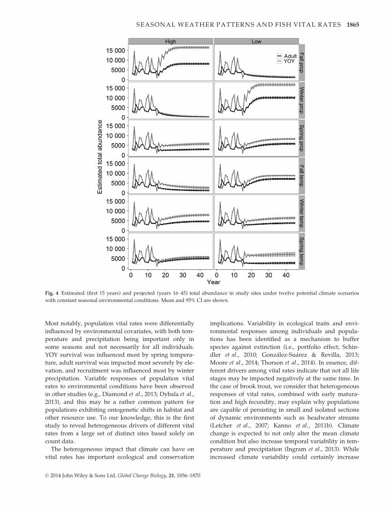
dance in our sites was projected to decline under low

fall precipitation, high winter precipitation, and high

fall temperature, with the first two weather conditions

exerting strong negative effects on abundance (Fig. 4).

This pattern emerged because low fall precipitation

and high winter precipitation had a strong negative

effect on recruitment (Table 2). Total adult abundance

was projected to be lower than or equal to total YOY

abundance in all scenarios (Fig. 4), which generally

mirrored the observed adult/YOY ratios between 1996

and 2010.

Population persistence depended on the frequencies

of high winter precipitation and varied among sites

due to the significant positive relationship between ele-

vation and adult survival (Table 2). In the scenario

where high winter flow occurred every 5 years, abun-

dance across sites showed a slightly increasing trend

(Fig. 5) and none of the local sites experienced quasi-

extinction (Fig. 6). Total abundance across sites

remained stable, and only one site experienced quasi-

extinction when high precipitation occurred for three

winters followed by two average winter conditions.

However, population decreases were projected at

greater frequencies of high winter precipitation; quasi-

extinction occurred in 13 sites when four of five winters

had high precipitation, and in approximately three

quarters of local sites (56 of 72 total sites) when high

winter precipitation occurred every year (Figs 5 and 6).

Elevation was an important determinant of extinction

risk. For example, quasi-extinction was predicted for

sites up to 532 m above sea level when high winter pre-

cipitation occurred every year, but it was predicted

only for sites lower than 408 m when four of five win-

ters were simulated to experience high precipitation.

Discussion

Brook trout populations responded to seasonal weather

patterns via complex pathways affecting vital rates.

Fig. 3 Mean (+ 95% CI) estimated annual total abundance in the 72 survey sites during 1996–2010. Solid lines indicate adult abundance,

and dotted lines indicate YOY abundance.

Table 3 Elasticity of population growth rate to a propor-

tional change in vital rates at three levels of local adult abun-

dance: low (10 individuals per 100 m), median (45

individuals), and high (121 individuals). Elasticity values (val-

ues in each column) sum to one (but they do not exactly sum

to one due to rounding of each value)

Local abundance

Low Median High

Per-capita recruitment 0.382 0.365 0.319

YOY survival 0.382 0.365 0.319

Adult survival 0.235 0.271 0.363



Most notably, population vital rates were differentially

influenced by environmental covariates, with both tem-

perature and precipitation being important only in

some seasons and not necessarily for all individuals.

YOY survival was influenced most by spring tempera-

ture, adult survival was impacted most severely by ele-

vation, and recruitment was influenced most by winter

precipitation. Variable responses of population vital

rates to environmental conditions have been observed

in other studies (e.g., Diamond et al., 2013; Dybala et al.,

2013), and this may be a rather common pattern for

populations exhibiting ontogenetic shifts in habitat and

other resource use. To our knowledge, this is the first

study to reveal heterogeneous drivers of different vital

rates from a large set of distinct sites based solely on

count data.

The heterogeneous impact that climate can have on

vital rates has important ecological and conservation

implications. Variability in ecological traits and envi-

ronmental responses among individuals and popula-

tions has been identified as a mechanism to buffer

species against extinction (i.e., portfolio effect; Schin-

dler et al., 2010; Gonz�alez-Su�arez & Revilla, 2013;

Moore et al., 2014; Thorson et al., 2014). In essence, dif-

ferent drivers among vital rates indicate that not all life

stages may be impacted negatively at the same time. In

the case of brook trout, we consider that heterogeneous

responses of vital rates, combined with early matura-

tion and high fecundity, may explain why populations

are capable of persisting in small and isolated sections

of dynamic environments such as headwater streams

(Letcher et al., 2007; Kanno et al., 2011b). Climate

change is expected to not only alter the mean climate

condition but also increase temporal variability in tem-

perature and precipitation (Ingram et al., 2013). While

increased climate variability could certainly increase

Fig. 4 Estimated (first 15 years) and projected (years 16–45) total abundance in study sites under twelve potential climate scenarios

with constant seasonal environmental conditions. Mean and 95% CI are shown.



temporal fluctuations in population abundance for each

life stage and render populations more susceptible to

local extirpation (Roland & Matter, 2013), heteroge-

neous responses among vital rates could also average

out individual patterns over a time period. The degree

of demographic synchrony and its effect on population

persistence should further be investigated for popula-

tions structured by age, size, and life stage across many

taxa.

Our study showed that the effect of temperature and

precipitation on vital rates depends on season. Warm

spring had a positive impact on YOY survival, but

Fig. 5 Estimated (first 15 years) and projected (years 16–45) total abundance in study sites under four potential high winter precipita-

tion conditions (mean + 1.5*SD) of varying frequencies. Mean and 95% CI are shown.

(a) (b) (c) (d)

Fig. 6 Local abundance trajectories in 72 survey sites under varying frequencies of high winter precipitation condition

(mean + 1.5*SD); (a) high winter precipitation occurs every 5 years, (b) three high precipitation winters followed by two average pre-

cipitation winters, (c) four high precipitation winters followed by one average precipitation winter, and (d) high winter precipitation

occurs every year. Each line represents mean estimated abundance at each of the 72 sites. For visual clarity, sites were classified as high

elevation (>600 m), mid-elevation (400–600 m), and low elevation (<400 m).



warm fall affected YOY survival negatively. Recruit-

ment was influenced positively by fall precipitation,

but negatively by winter precipitation. The latter find-

ing indicates that seasonal distributions of precipitation

amount can affect brook trout populations even though

total precipitation remains unchanged. These results

suggest that our examination of population vital rates

across seasons provided novel insights of population

responses to changing climate, and this knowledge

would be required for accurate prediction of popula-

tion persistence.

High winter precipitation strongly affected the popu-

lation dynamics of brook trout in our study. Climate

change impacts on wild animal populations have been

most commonly examined using annual or single-sea-

son temperature values (e.g., Roland & Matter, 2013;

Wenger et al., 2013; Dueri et al., 2014). For example,

potential changes in geographic distributions of cold-

water salmonids have been projected based on altera-

tions in annual mean temperature (Flebbe et al., 2006;

Zeiger et al., 2012) and summer mean temperature

(Roberts et al., 2013; Wenger et al., 2013). Although

summer weather is important for a coldwater species

such as brook trout and the omission of summer

weather patterns is a potential caveat in our study, we

found that changes in winter precipitation can also

drive local populations to extirpation. We suspect that

high winter flow is associated with recruitment failures

because fertilized eggs remain in the gravel during this

period and are susceptible to bed scouring (Petty et al.,

2005; Wenger et al., 2013). The finding that winter

weather can potentially be a major driving force in pop-

ulation trajectories was unexpected as stenothermal

ectotherm species are typically considered to be regu-

lated by temperature regimes. Interestingly, the winter

weather pattern, particularly air temperature, is

expected to change more than any other season in

many climate change projections (Ingram et al., 2013).

Warmer winter would increase the amount of rain,

instead of snow, which may exacerbate the winter flow

impact on brook trout population dynamics in the

future climate.

While high winter precipitation affected trout popu-

lations negatively, our simulations indicated that the

frequency of such conditions could determine popula-

tion trajectories. Quasi-extinction was projected to

occur at three quarters of survey sites when high winter

precipitation conditions were simulated every year, but

population abundance did not show a clear sign of

decline (only one local site with quasi-extinction) when

at least two of five winters were simulated to experi-

ence mean winter precipitation conditions. This pattern

emerged due partly to density-dependent recruitment.

Density-dependent responses of vital rates have been

linked to stability and resiliency in brook trout (Gross-

man et al., 2010, 2012) and other animal populations

(Kruger, 2007; Reed & Slade, 2008). Density-dependent

processes can potentially play a major role in popula-

tion viability under climate change scenarios where cli-

mate variability is predicted to increase (Ingram et al.,

2013; Rummukainen, 2013) and animals are more likely

to experience a combination of favorable and unfavor-

able conditions across years. A critical question for

future work then is: ‘Can positive effects of some favor-

able years on population abundance offset negative

impacts of unfavorable years?’

Elevation played an important role in determining

variation in the likelihood of population persistence

among sites. It was not surprising that brook trout pop-

ulations were more likely to persist at higher elevation

sites under altered climate conditions; similar altitude-

mediated effects have been consistently found in ani-

mals and plants under climate change projections (Loa-

rie et al., 2009; Chen et al., 2011; Wenger et al., 2013).

However, a new perspective offered in the current

work is that this pattern resulted from higher adult sur-

vival at high-elevation sites, a demographic mechanism

that would not have been apparent based solely on

analysis of geographic distributions or abundance.

Although adult survival was important in explaining

heterogeneity among sites, population growth rate was

most sensitive to recruitment and YOY survival unless

adult abundance was high. The same conclusion has

been drawn from other studies of headwater brook

trout populations (Marschall & Crowder, 1996; Letcher

et al., 2007), and this is common among short-lived

freshwater fish species (V�elez-Espino et al., 2006). These

complex demographic patterns further suggest a need

for understanding how vital rates in stage-structured

populations differentially respond to environmental

change.

There are few long-term monitoring data sets in

animal population ecology. Monitoring designs

should be carefully considered when an opportunity

exists to collect such data. There remains an impor-

tant question about the optimal spatial and temporal

distributions of sampling effort. While only two of

72 study sites were surveyed every year during the

15-year study period, different sets of additional

sites were surveyed in consecutive years throughout

the study period. We consider that the judicious

inclusion of consecutive years greatly improved our

inferences on temporal variation in population vital

rates. Zipkin et al. (2014a) found that increasing the

number of years surveyed resulted in more accurate

and precise parameter estimates in simulations of

the open population N-mixture model; for example,

known population vital rates were recovered



accurately with only five sites when data were sim-

ulated for 20 years. In addition, a combination of

single-pass (16%) and three-pass (84%) depletion

surveys allowed us to estimate stage-specific detec-

tion probability. Because electrofishing is size selec-

tive, accounting for the potential differences in

detection probabilities for YOY and adults was nec-

essary for accurate inferences. Our work represented

a case study in which a flexible modeling frame-

work was successfully applied to missing or imper-

fect long-term data to make inferences on key vital

rates that differed across space, time, and stages.

This modeling framework is a powerful approach

because it can incorporate demographic processes at

a broad spatial scale and can provide researchers

and managers with an innovative tool to link

demography to landscape-level conservation efforts.

The current work adds to a growing list of studies

that attempt to estimate vital rates in structured popu-

lations using count data (Link et al., 2003; Dail & Mad-

sen, 2011; Zipkin et al., 2014a). While we highlighted its

strengths in this study, we also recognize the limita-

tions. Importantly, analyses of count data are less capa-

ble of making inferences on complex population

dynamics compared to traditional mark–recapturemethods. Zipkin et al. (2014b) applied a similar state-

structured population model to black-throated blue

warblers (Setophaga caerulescens) populations, in which

survival probabilities were estimated for each life stage

and sex. Survival probabilities tended to be underesti-

mated when compared to inferences based on mark–recapture data. Accounting for immigration appears to

be another challenge in count data. Zipkin et al. (2014a)

used simulated data sets and an empirical data set on a

highly immobile stream amphibian (northern dusky

salamanders Desmognathus fuscus) and demonstrated

that immigration and apparent survival could be esti-

mated simultaneously in stage-structured populations

from count data. Such models did not converge or

model outputs were sensitive to a slight change in

model structures in SNP brook trout data (Y. Kanno &

D.A. Boughton, unpublished data). As a result, we

could not explicitly account for immigration in this

study. Zipkin et al. (2014b) similarly noted that count

data may not contain enough demographic information

for estimating all parameters in some cases and sug-

gested an integration of mark–recapture and count data

as an efficient modeling approach for estimating vital

rates (e.g., Schaub & Abadi, 2011; Oppel et al., 2014). In

our case, a more structurally complex model than pre-

sented here would not be necessary for our goal of

identifying key demographic drivers of population

responses to seasonal weather patterns. However, if the

goal were to understand the relative importance of

immigration versus apparent survival in a meta-popu-

lation study, a more complex model with additional

data sources (e.g., mark–recapture data at a limited

number of sites) would be necessary. Our modeling

approach is indeed flexible enough to accommodate

such additional structures, and future research is much

needed to provide a framework in which multiple data

sources are integrated for ecological inferences at

broader spatial and temporal scales.

Acknowledgements

We thank the National Park Service Inventory and MonitoringProgram and more specifically Jim Atkinson and David Dema-rest for their efforts in the field. This manuscript is a contribu-tion from a working group at the John Wesley Powell Center forAnalysis and Synthesis, funded by the US Geological Survey.An earlier version of this manuscript was greatly improved byconstructive comments from two anonymous reviewers.

References

Alonso C, de Jaløn DG, �Alvarez J, Gort�azar J (2011) A large-scale approach can help

detect general processes driving the dynamics of brown trout populations in

extensive areas. Ecology of Freshwater Fish, 20, 449–460.

Anglin ZW, Grossman GD (2013) Microhabitat use by southern brook trout (Salveli-

nus fontinalis) in a headwater North Carolina stream. Ecology of Freshwater Fish, 22,

567–577.

Arismendi I, Johnson SL, Dunham JB, Haggerty R (2013) Descriptors of natural ther-

mal regimes in streams and their responsiveness to change in the Pacific North-

west of North America. Freshwater Biology, 58, 880–894.

Berger AM, Gresswell RE (2009) Factors influencing coastal cutthroat trout (Oncorhyn-

chus clarkii clarkii) seasonal survival rates: a spatially continuous approach within

stream networks. Canadian Journal of Fisheries and Aquatic Sciences, 66, 613–632.

Blanchfield PJ, Ridgway MS (2005) The relative influence of breeding competition

and habitat quality on female reproductive success in lacustrine brook trout (Salv-

elinus fontinalis). Canadian Journal of Fisheries and Aquatic Sciences, 62, 2694–2705.

Boss SM, Richardson JS (2002) Effects of food and cover on the growth, survival, and

movement of cutthroat trout (Oncorhynchus clarki) in coastal streams. Canadian

Journal of Fisheries and Aquatic Sciences, 59, 1044–1053.

Carline RF, McCullough BJ (2003) Effects of floods on brook trout populations in the

Monongahela National Forest, West Virginia. Transactions of the American Fisheries

Society, 132, 1014–1020.

Carlson SM, Olsen EM, Vøllestad LA (2008) Seasonal mortality and the effect of body

size: a review and an empirical test using individual data on brown trout. Func-

tional Ecology, 22, 663–673.

Chen IC, Hill JK, Ohlemuller R, Roy DB, Thomas CD (2011) Rapid range shifts of spe-

cies associated with high levels of climate warming. Science, 333, 102–1026.

Dail D, Madsen L (2011) Models for estimating abundance from repeated counts of

an open metapopulation. Biometrics, 67, 577–587.

Diamond SL, Murphy CA, Rose KA (2013) Simulating the effects of global climate

change on Atlantic croaker population dynamics in the mid-Atlantic Region. Eco-

logical Modelling, 264, 98–114.

Dueri S, Bopp L, Maury O (2014) Projecting the impacts of climate change on skipjack

tuna abundance and spatial distribution. Global Change Biology, 20, 742–753.

Dybala KE, Eadie JM, Gardali T, Seavy NE, Herzog MP (2013) Projecting demo-

graphic responses to climate change: adult and juvenile survival respond differ-

ently to direct and indirect effects of weather in a passerine population. Global

Change Biology, 19, 2688–2697.

Essington TE, Sorensen PW, Paron DG (1998) High rate of redd superimposition by

brook trout (Salvelinus fontinalis) and brown trout (Salmo trutta) in a Minnesota

stream cannot be explained by habitat availability alone. Canadian Journal of Fisher-

ies and Aquatic Sciences, 55, 2310–2316.

Falke JA, Fausch KD, Bestgen KR, Bailey LL (2010) Spawning phenology and habitat

use in a Great Plains, USA, stream fish assemblage: an occupancy estimation

approach. Canadian Journal of Fisheries and Aquatic Sciences, 67, 1942–1956.



Fern�andez-Chac�on A, Bertolero A, Amengual A, Tavecchia G, Homar V, Oro D

(2011) Spatial heterogeneity in the effects of climate change on the population

dynamics of a Mediterranean tortoise. Global Change Biology, 17, 3075–3088.

Flebbe PA, Roghair LD, Bruggink JL (2006) Spatial modeling to project southern

Appalachian trout distribution in a warmer climate. Transactions of the American

Fisheries Society, 135, 1371–1382.

Gelman A (2003) A Bayesian formulation of exploratory data analysis and goodness-

of-fit testing. International Statistical Review, 71, 369–382.

Gelman A, Hill J (2007) Data Analysis Using Regression and Multilevel/Hierarchical Mod-

els. Cambridge University Press, New York.

Gonz�alez-Su�arez M, Revilla E (2013) Variability in life-history and ecological traits is

a buffer against extinction in mammals. Ecology Letters, 16, 242–251.

Gross K, Craig BA, Huchison WD (2002) Bayesian estimation of a demographic

matrix model from stage-frequency data. Ecology, 83, 3285–3298.

Grossman GD, Ratajczak RE, Wagner CM, Petty JT (2010) Dynamics and regulation

of the southern brook trout (Salvelinus fontinalis) population in an Appalachian

stream. Freshwater Biology, 55, 1494–1508.

Grossman GD, Nuhfer A, Zorn T, Sundin G, Alexander G (2012) Population regula-

tion of brook trout (Salvelinus fontinalis) in Hunt Creek, Michigan: a 50-year study.

Freshwater Biology, 57, 1434–1448.

Hakala JP, Hartman KJ (2004) Drought effect on stream morphology and brook trout

(Salvelinus fontinalis) populations in forested headwater streams. Hydrobiologia,

515, 203–213.

Hartman KJ, Cox MK (2008) Refinement and testing of a brook trout bioenergetics

model. Transactions of the American Fisheries Society, 137, 357–363.

Haslob H, Hauss H, Petereit C, Clemmesen C, Kraus G, Peck MA (2012) Temperature

effects on vital rates of different life stages and implications for population growth

of Baltic sprat. Marine Biology, 159, 2621–2632.

Hegel TM, Mysterud A, Ergon T, Loe LE, Huettmann F, Stenseth NC (2010) Seasonal

effects of Pacific-based climate on recruitment in a predator-limited large herbi-

vore. Journal of Animal Ecology, 79, 471–482.

Heisler LM, Somers CM, Poulin RG (2014) Rodent populations on the northern Great

Plains respond to weather variation at a landscape scale. Journal of Mammalogy, 95,

82–90.

Hilborn R, Walters CJ (1992) Quantitative Fisheries Stock Assessment: Choice, Dynamics

and Uncertainty. Chapman and Hall, New York.

Hudy M, Thieling TM, Gillespie N, Smith EP (2008) Distribution, status, and land use

characteristics of subwatersheds within the native range of brook trout in the east-

ern United States. North American Journal of Fisheries Management, 28, 1069–1085.

Hudy M, Coombs JA, Nislow KH, Letcher BH (2010) Dispersal and within-stream

spatial population structure of brook trout revealed by pedigree reconstruction.

Transactions of the American Fisheries Society, 139, 1276–1287.

Hunter CM, Caswell H, Runge MC, Regehr EV, Amstrup SC, Stirling I (2010) Climate

change threatens polar bear populations: a stochastic demographic analysis. Ecol-

ogy, 91, 2883–2897.

Huntington TG, Richardson AD, McGuire KJ, Hayhoe K (2009) Climate and

hydrological changes in the northeastern United States: recent trends and implica-

tions for forested and aquatic ecosystems. Canadian Journal of Forest Research, 39,

199–212.

Ingram KT, Dow K, Carter L, Anderson J (2013) Climate of the Southeastern United

States: Variability, Change, Impacts, and Vulnerability. Island Press, Washington, DC.

Jastram JD, Snyder CD, Hitt NP, Rice KC (2013) Synthesis and interpretation of surface-

water quality and aquatic biota collected in Shenandoah National Park, Virginia, 1979–

2009. Scientific Investigations Report 2013-5157. US Geological Survey, Reston, Vir-

ginia.

Jenouvrier S, Thibault JC, Viallefont A et al. (2009) Global climate patterns explain

range-wide synchrony in survival of a migratory bird. Global Change Biology, 15,

268–279.

Jensen AJ, Johnsen BO (1999) The functional relationship between peak spring floods

and survival and growth of juvenile Atlantic salmon (Salmo salar) and brown trout

(Salmo trutta). Functional Ecology, 13, 778–785.

Kanno Y, Vokoun JC, Letcher BH (2011a) Sibship reconstruction for inferring mating

systems, dispersal and effective population size in headwater brook trout (Salveli-

nus fontinalis) populations. Conservation Genetics, 12, 619–628.

Kanno Y, Vokoun JC, Letcher BH (2011b) Fine-scale population structure and river-

scape genetics of brook trout (Salvelinus fontinalis) distributed continuously along

headwater channel networks. Molecular Ecology, 20, 3711–3729.

Kanno Y, Vokoun JC, Holsinger KE, Letcher BH (2012) Estimating size-specific brook

trout abundance in continuously sampled headwater streams using Bayesian

mixed models with zero inflation and overdispersion. Ecology of Freshwater Fish,

21, 404–419.

Kanno Y, Letcher BH, Vokoun JC, Zipkin EF (2014) Spatial variability in adult brook

trout (Salvelinus fontinalis) survival within two intensively surveyed headwater

stream networks. Canadian Journal of Fisheries and Aquatic Sciences, 71, 1010–1019.

K�ery M, Schaub M (2012) Bayesian Population Analysis Using WinBUGS: A Hierarchical

Perspective. Elsevier, Amsterdam.

Kruger O (2007) Long-term demographic analysis in goshawk Accipiter gentilis: the

role of density dependence and stochasticity. Oecologia, 152, 459–471.

Lack D (1954) The Natural Regulation of Animal Numbers. Clarendon Press, Oxford,

UK.

Letcher BH, Nislow KH, Coombs JA, O’Donnell MJ, Dubreuil TL (2007) Population

response to habitat fragmentation in a stream-dwelling brook trout population.

PLoS ONE, 2, e1139.

Link WA, Royle JA, Hatfield JS (2003) Demographic analysis from summaries of an

age-structured population. Biometrics, 59, 778–785.

Loarie SR, Duffy PB, Hamilton H, Asner GP, Field CB, Ackerly DD (2009) The veloc-

ity of climate change. Nature, 462, 1052–1055.

Lobøn-Cervi�a J (2014) Recruitment and survival rate variability in fish populations:

density-dependent regulation or further evidence of environmental determinants?

Canadian Journal of Fisheries and Aquatic Sciences, 71, 290–300.

Lok T, Overdijk O, Tinbergen JM, Piersma T (2013) Seasonal variation in density

dependence in age-specific survival of a long-distance migrant. Ecology, 94, 2358–

2369.

Maceina MJ, Pereira DL (2007) Recruitment. In: Analysis and Interpretation of Freshwa-

ter Fisheries Data, 1st edn (eds Guy CS, Brown ML), pp. 121–185. American Fisher-

ies Society, Bethesda, MD.

Marschall EA, Crowder LB (1996) Assessing population responses to multiple anthro-

pogenic effects: a case study with brook trout. Ecological Applications, 6, 152–167.

McCargo JW, Peterson JT (2010) An evaluation of the influence of seasonal base flow

and geomorphic characteristics on coastal plain stream fish assemblages. Transac-

tions of the American Fisheries Society, 139, 29–48.

McKenna JE Jr, Johnson JH (2011) Landscape models of brook trout abundance and

distribution in lotic habitat with field validation. North American Journal of Fisheries

Management, 31, 742–756.

Moore JW, Yeakel JD, Peard D, Lough J, Beere M (2014) Life-history diversity and its

importance to population stability and persistence of a migratory fish: steelhead in

two large North American watersheds. Journal of Animal Ecology, 83, 1035–1046.

Nicola GG, Almod�ovar A, Jonsson B, Elvira B (2008) Recruitment variability of resi-

dent brown trout in peripheral populations from southern Europe. Freshwater Biol-

ogy, 53, 2364–2474.

Nilsson ALK, Knudsen E, Jerstad K, Røstad OW, Walseng B, Slagsvold T, Stenseth

NC (2011) Climate effects on population fluctuations of the white-throated dipper

Cinclus cinclus. Journal of Animal Ecology, 80, 235–243.

Novotny EV, Stefan HG (2007) Stream flow in Minnesota: indicator of climate change.

Journal of Hydrology, 334, 319–333.

Oppel S, Hilton G, Ratcliffe N et al. (2014) Assessing population viability while

accounting for demographic and environmental uncertainty. Ecology, 95, 1809–1818.

Perry GLW, Bond NR (2009) Spatially explicit modelling of habitat dynamics and fish

populations persistence in an intermittent lowland stream. Ecological Applications,

19, 731–746.

Petty JT, Lamothe PJ, Mazik PM (2005) Spatial and seasonal dynamics of brook trout

populations inhabiting a central Appalachian watershed. Transactions of the Ameri-

can Fisheries Society, 134, 572–587.

Plummer M (2003) JAGS: a program for analysis of Bayesian graphical models using

Gibbs sampling. Proceedings of the third International Workshop on Distributed

Statistical Computing (DSC 2003), March 20-22. Vienna, Austria.

Plummer M (2011) rjags: Bayesian graphical models using MCMC. R package version

2.2.0-4. http://cran.r-project.org/web/packages/rjags/

Poff NL, Allan JD, Bain MB et al. (1997) The natural flow regime: a new paradigm for

river conservation and restoration. BioScience, 47, 769–784.

R Development Core Team (2013) R: A Language and Environment for Statistical Com-

puting. R Foundation for Statistical Computing. Vienna, Austria.

Reed AW, Slade NA (2008) Density-dependent recruitment in grassland small mam-

mals. Journal of Animal Ecology, 77, 57–65.

Reynolds JB, Kolz AL (2012) Electrofishing. In: Fisheries Techniques (eds Zale AV, Par-

rish DL, Sutton TM), pp. 305–361. American Fisheries Society, Bethesda, MD.

Richards JM, Hansen MJ, Bronte CR, Sitar SP (2004) Recruitment dynamics of the

1971–1991 year-classes of lake trout in Michigan waters of Lake Superior. North

American Journal of Fisheries Management, 24, 475–489.

Roberts JJ, Fausch KD, Peterson DP, Hooten MB (2013) Fragmentation and thermal

risks from climate change interact to affect persistence of native trout in the Colo-

rado River basin. Global Change Biology, 19, 1383–1398.



http://cran.r-project.org/web/packages/rjags/

Roghair CN, Dolloff CA, Underwood MK (2002) Response of a brook trout popula-

tion and instream habitat to a catastrophic flood and debris flow. Transactions of

the American Fisheries Society, 131, 718–730.

Roland J, Matter SF (2013) Variability in winter climate and winter extremes reduces

population growth of an alpine butterfly. Ecology, 94, 190–199.

Roth T, Plattner M, Amrhein V (2014) Plants, birds and butterflies: short-term

responses of species communities to climate warming vary by taxon and with alti-

tude. PLoS ONE, 9, e82490.

Royle JA (2004) N-mixture models for estimating population size from spatially repli-

cated counts. Biometrics, 60, 108–115.

Rummukainen M (2013) Climate change: changing means and changing extremes.

Climatic Change, 121, 3–13.

Schaub M, Abadi F (2011) Integrated population models: a novel analysis framework

for deeper insights into population dynamics. Journal of Ornithology, 152 (Supple-

ment), 227–237.

Schindler DE, Hilborn R, Chasco B, Boatright CP, Quinn TP, Rogers LA, Webster MS

(2010) Population diversity and the portfolio effect in an exploited species. Nature,

465, 609–612.

Spiegelhalter DJ, Best NG, Carlin BR, van der Linde A (2002) Bayesian measures of

model complexity and fit. Journal of the Royal Statistical Society Series B (Statistical

Methodology), 64, 583–616.

Stubben CJ, Milligan BG (2007) Estimating and analyzing demographic models using

the popbio package in R. Journal of Statistical Software, 22, 11.

Thomas CD, Cameron A, Green RE et al. (2004) Extinction risk from climate change.

Nature, 427, 145–148.

Thorson JT, Scheuerell MD, Buhle ER, Copeland T (2014) Spatial variation buffers

temporal fluctuations in early juvenile survival for an endangered Pacific salmon.

Journal of Animal Ecology, 83, 157–167.

V�elez-Espino LA, Fox MG, McLaughlin RL (2006) Characterization of elasticity pat-

terns of North American freshwater fishes. Canadian Journal of Fisheries and Aquatic

Sciences, 63, 2050–2066.

Vindenes Y, Edeline E, Ohlberger J, Langangen O, Winfield IJ, Stenseth NC, Vøllestad

LA (2014) Effects of climate change on trait-based dynamics of a top predator in

freshwater ecosystems. The American Naturalist, 183, 243–256.

Warren DR, Robinson JM, Josephson DC, Sheldon DR, Kraft CE (2012) Elevated sum-

mer temperatures delay spawning and reduce redd construction for resident

brook trout (Salvelinus fontinalis). Global Change Biology, 18, 1804–1811.

Wenger SJ, Som NA, Dauwalter DC et al. (2013) Probabilistic accounting of uncer-

tainty in forecasts of species distributions under climate change. Global Change

Biology, 19, 3343–3354.

Werner EE, Gilliam JF (1984) The ontogenetic niche and species interactions in size-

structured populations. Annual Review of Ecology and Systematics, 15, 393–425.

Williams BK, Nichols JD, Conroy MJ (2002) Analysis and Management of Animal Popula-

tions. Academic Press, San Diego, CA.

Wright LJ, Hoblyn RA, Green RE, Bowden CGR, Mallord JW, Sutherland WJ, Dolman

PM (2009) Importance of climatic and environmental change in the demography

of a multi-brooded passerine, the woodlark Lullula arborea. Journal of Animal Ecol-

ogy, 78, 1191–1202.

Xu C, Letcher BH, Nislow KH (2010a) Size-dependent survival of brook trout Salveli-

nus fontinalis in summer: effects of water temperature and stream flow. Journal of

Fish Biology, 76, 2342–2369.

Xu C, Letcher BH, Nislow KH (2010b) Context-specific influence of water tempera-

ture on brook trout growth rates in the field. Freshwater Biology, 55, 2253–2264.

Zeiger MP, Todd AS, Cadwell CA (2012) Evidence of recent climate change within

the historic range of Rio Grande cutthroat trout: implications for management and

future persistence. Transactions of the American Fisheries Society, 141, 1045–1059.

Zipkin EF, Thorson JT, See K et al. (2014a) Modeling structured population dynamics

using data from unmarked individuals. Ecology, 95, 22–29.

Zipkin EF, Sillett TS, Grant EHC, Chandler RB, Royle JA (2014b) Inferences about

population dynamics from count data using multistate models: a comparison to

capture-recapture approaches. Ecology and Evolution, 4, 417–426.

Supporting Information

Additional Supporting Information may be found in theonline version of this article:

Appendix S1. Brook trout length-frequency histograms.Appendix S2. Spawner-recruit relationship.Appendix S3. May to August stream flow.Appendix S4. JAGS code.Appendix S5. Model selection steps.Appendix S6. Model diagnostics.



Documents

Seasonal weather patterns drive population vital rates and …sites.warnercnr.colostate.edu/kanno/wp-content/uploads/sites/112/2… · (Salvelinus fontinalis) at a broad spatial scale