Seasonal cycle as template for climate variability on

Seasonal cycle as template for climate variability on astronomical

timescales

Thomas Laepple1 and Gerrit Lohmann1

Received 11 August 2008; revised 22 June 2009; accepted 2 July 2009; published 13 October 2009.

[1] We propose a new concept for insolation-driven temperature variability on orbital timescales. It relies onthe modern relationship between insolation and temperature throughout the year. The method consists of(1) estimating empirical transfer functions between daily insolation and daily temperature and (2) applying thesetransfer functions on the long-term insolation to model the late Quaternary temperature evolution. On the basisof the observed insolation-temperature relationship, different temperature response regimes across the Earth areidentified. Linear relationships dominate extratropical land areas whereas in midlatitude oceans, the seasonallyvarying mixed layer depth renders the temperature more sensitive to summer than to winter insolation. Thetemperature in monsoon regions and regions of seasonal sea ice cover also shows a seasonally varying responseto insolation. These transfer functions characterize the shape of the seasonal cycle in temperature and influencethe temperature evolution on orbital timescales by rectifying the insolation signal. On the basis of our seasonaltemplate model, we estimate the temperature evolution of the last 750,000 years. The model largely reproducesthe Holocene temperature trends as simulated by a coupled climate model. In the frequency domain, significanttemperature variability in the eccentricity and semiprecession frequency band in the tropics is found.Midlatitudes are dominated by precession, and high latitudes are dominated by obliquity. Further, it is found thatthe expected frequency response highly depends on the location. Our local time-independent approachcomplements the global Milankovitch hypothesis (climate variations are driven by northern summer insolation)in explaining observed climate variability and potentially offers new insights in interpreting paleoclimaterecords.

Citation: Laepple, T., and G. Lohmann (2009), Seasonal cycle as template for climate variability on astronomical timescales,

Paleoceanography, 24, PA4201, doi:10.1029/2008PA001674.

1. Introduction

[2] The incoming solar radiation at the top of the atmo-sphere varies during the seasonal cycle as well as onmultimillennial timescales. The long-term variations arecaused by changes in the Earth’s orbital geometry thataffect the seasonal and latitudinal distribution of insolation.By computational analysis of the planetary system, thesevariations can be calculated to a high accuracy for the lastmillions of years [Berger and Loutre, 1991; Berger, 1978;Laskar et al., 2004].[3] Apart from shaping the seasonal cycle, the changes in

the seasonal and latitudinal distribution of solar radiation area primary driver for climate variability on multimillennialtimescales. This relationship has been hypothesized for along time [Adhemar, 1842; Croll, 1875; Milankovitch,1941], and coherent variability of climate records andorbital parameters was found when geologists started todate climatic proxy records of ocean sediments [e.g.,Broecker and van Donk, 1970; Hays et al., 1976]. Despiteimportant advances in the research of the orbitally forced

climate variability the question remains how the climatesystem reacts on insolation forcing.[4] One classical concept for the response of the climate

system on orbital forcing was proposed by SPECMAP[Imbrie et al., 1992]. Investigating a wide range of sedimentcores, the authors concluded that insolation changes at highnorthern latitudes initiate a sequence of climate responsesstarting in the north, propagating to the south, and laterreturning north to force the ice sheets. Recent studies basedon proxy data and models challenge this ‘‘northern pacing’’viewpoint and suggest that local insolation at differentlatitudes also plays an important role. One example is thesensitivity of the climate in the tropical Pacific Ocean tolocal insolation that may influence the global climate [e.g.,Cane, 1998]; In addition, proxy records from ocean sedi-ment cores, representing the sea surface temperature (SST)show a different pattern between low and high latitudes[Pahnke and Sachs, 2006]; Modeling work shows thattemperature variability in Antarctica may be driven by localinsolation [Huybers and Denton, 2008]; Studies fromcoupled atmosphere-ocean general circulation models(AOGCM) suggest that the strength of the monsoons isinfluenced by local insolation [e.g., Clemens et al., 1991]; Arecent study compared transient AOGCM simulations of theHolocene with temperature proxy data [Lorenz et al., 2006]and emphasized the heterogeneous pattern of the tempera-ture response to insolation forcing.

PALEOCEANOGRAPHY, VOL. 24, PA4201, doi:10.1029/2008PA001674, 2009ClickHere

for

FullArticle

1Alfred Wegener Institute for Polar and Marine Research, Bremerhaven,Germany.

Copyright 2009 by the American Geophysical Union.0883-8305/09/2008PA001674$12.00

PA4201 1 of 15

http://dx.doi.org/10.1029/2008PA001674

[5] The climate response to insolation is nonlinear:Variations, coherent to the precession of the perihelion arefound in a large number of temperature proxies [e.g., Imbrieet al., 1992; Pahnke et al., 2003], but the precession of theperihelion does not affect the annual mean insolation atany point on Earth [Rubincam, 1994]. One particularnonlinearity is proposed in the classical studies ofMilankovitch [1941] and SPECMAP [Imbrie et al., 1992]who state that the summer insolation intensity is the drivingforce linking the sensitivity of snow ablation to summerradiation. This concept was refined by the summer energyconcept of Huybers [2006] and Huybers and Tziperman[2008] who point to the role of the integrated summerinsolation as driver of snow ablation. Part of the glacial-interglacial variability can be understood by these concepts.However, it seems unlikely that summer is the dominatingseason on all orbital timescales and in all regions.[6] Hence, nonlinear and spatially resolved models are

needed for the understanding of the climate response oninsolation forcing. For this purpose energy balance modelswere used and could show the important role of the land-seadistribution on the orbital temperature variability found inproxy records [Short et al., 1991]. However, importantfeedback mechanisms were neglected by using a linearapproach. On the other hand, three-dimensional climatemodels provide a physically consistent approach and showthe importance of the local forcing, especially in the tropics[e.g., Clement et al., 2004; Tuenter et al., 2003]. However,climate model simulations are limited in length by computingresources. Further, a simulation from a complex modeldoes not imply a direct understanding of the mechanismsinvolved [Held, 2005].[7] Here we make use of the modern seasonal cycle of

temperature to derive the insolation-temperature relation-ship on reanalysis data. We propose a simple concept: thelocal temperature response to insolation has the sametransfer function on astronomical timescales and on seasonaltime scales. Our method consists of (1) estimating empiricaltransfer functions between daily insolation and dailytemperature and (2) applying these transfer functions onthe long-term insolation history to model the past temper-ature evolution. Our technique includes nonlinearities thatare shaping the modern seasonal cycle to derive a localmodel for the temperature response. Since the method doesnot include slow feedbacks such as the ablation of icesheets, that is a multiyear process, or feedbacks caused bythe interaction of the carbon cycle and the climate system,it cannot be used to estimate glacial-interglacial climatevariability. However, the empirical approach includes all‘‘fast’’ feedback (seasonal time scale) processes and allowsa systematic estimation of their influence on the regionaltemperature evolution of the Quaternary.

2. Data and Methods

2.1. Temperature Data and Holocene ModelSimulation

[8] To derive the present-day temperature cycle, we usedaily near-surface temperature data from the NationalCenters for Environmental Prediction (NCEP) reanalysis

[Kalnay et al., 1996]. The data are available on a 2.5 � 2.5�horizontal grid, and we examine the mean seasonal cyclederived from the years 1948–2007 after removing the leapdays. For the comparison of our technique with complexclimate models, we use a transient simulation from theatmosphere-ocean general circulation model ECHO–G[Lorenz et al., 2006; Lorenz and Lohmann, 2004]. Thissimulation covers the last 7000 years from the mid-Holoceneuntil today, changing only the orbital forcing. It consists ofa two member simulation, performed with a 10 timesaccelerated insolation forcing (700 model years). In ourstudy, we analyze the near-surface temperature and the seaice coverage averaged over the two ensemble members.

2.2. Parameterizing the Temperature Responseto Insolation

[9] The annual cycle of surface temperature can beapproximated as a linear function of insolation afterincluding a time lag to represent the thermal inertia [e.g.,Huybers, 2006]:

Tsurf t; xð Þ ¼ a xð Þ þ b xð Þ * I t � t xð Þ; xð Þ ð1Þ

Here Tsurf is the surface temperature, I the insolation, t thetime of the year, x the location, a is a free parameter, brepresents the linear temperature sensitivity and t the timelag between insolation and temperature.[10] Because in some regions the local temperature is

more sensitive to summer or winter insolation we introducea nonlinear extension of this model by applying a polynomialtransfer function between temperature and insolation. Thetemperature is now modeled as

Tsurf t; xð Þ ¼ F I t � t xð Þ; xð Þð Þ withF I ; xð Þ ¼ a xð Þ þ b xð ÞI þ c xð ÞI2 þ d xð ÞI3 ð2Þ

The coefficients a .. d as well as t are determined by a leastsquares fit on the daily data. In preliminary studies, wefound a third-order polynomial to be a tradeoff betweenexplained variance and model complexity. The results arenot sensitive to this choice, as similar results are obtainedusing a second- or fourth-order polynomial.[11] We estimate the linear and polynomial transfer func-

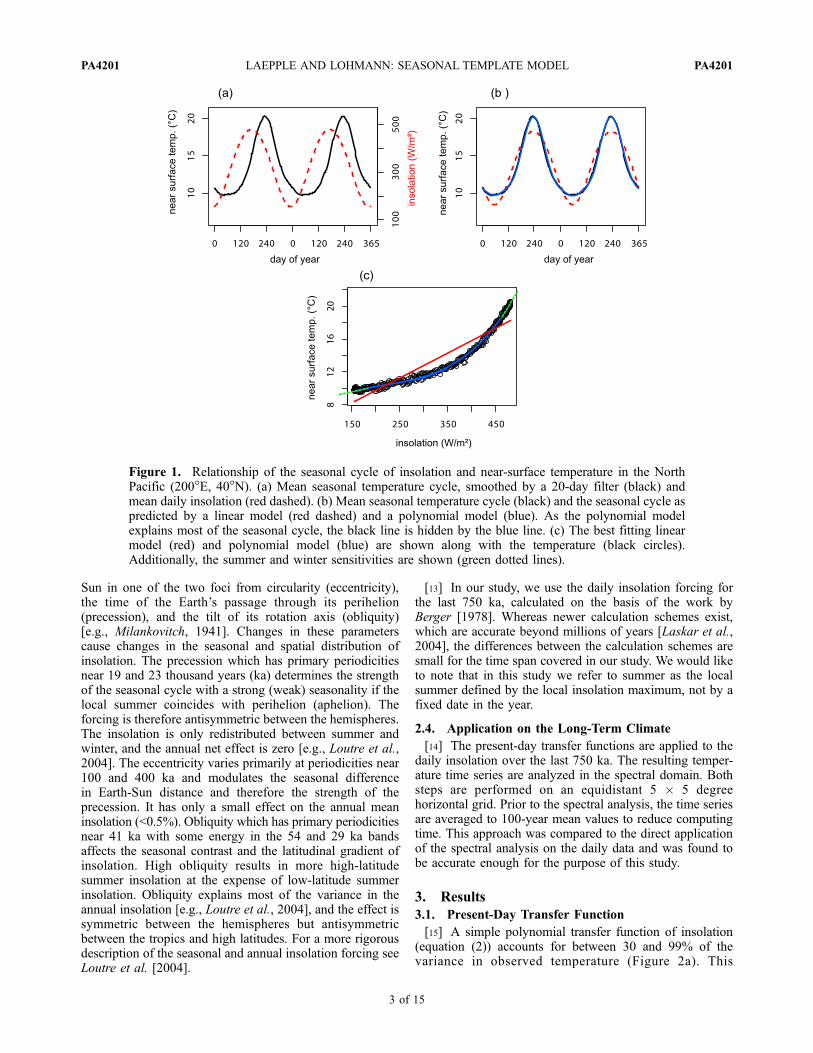
tions between local insolation and local surface temperatureon a 5 � 5 degree horizontal grid, using daily reanalysisdata. The approach is demonstrated for one grid point in theNorth Pacific (40�N 200�E) (Figure 1). At this location, thetemperature lags insolation by approximately two months,and the summer temperature highs and winter temperaturelows are narrower and broader, respectively, than thosein insolation. Therefore, only a polynomial model canaccurately represent the temperature cycle as function ofthe insolation cycle. The transfer function shows a nonlinearbehavior with smaller temperature sensitivity in winter thanin summer.

2.3. Insolation Forcing

[12] The orbital forcing is controlled by three mainparameters: the departure of the elliptical orbit with the

PA4201 LAEPPLE AND LOHMANN: SEASONAL TEMPLATE MODEL

2 of 15

PA4201

Sun in one of the two foci from circularity (eccentricity),the time of the Earth’s passage through its perihelion(precession), and the tilt of its rotation axis (obliquity)[e.g., Milankovitch, 1941]. Changes in these parameterscause changes in the seasonal and spatial distribution ofinsolation. The precession which has primary periodicitiesnear 19 and 23 thousand years (ka) determines the strengthof the seasonal cycle with a strong (weak) seasonality if thelocal summer coincides with perihelion (aphelion). Theforcing is therefore antisymmetric between the hemispheres.The insolation is only redistributed between summer andwinter, and the annual net effect is zero [e.g., Loutre et al.,2004]. The eccentricity varies primarily at periodicities near100 and 400 ka and modulates the seasonal differencein Earth-Sun distance and therefore the strength of theprecession. It has only a small effect on the annual meaninsolation (<0.5%). Obliquity which has primary periodicitiesnear 41 ka with some energy in the 54 and 29 ka bandsaffects the seasonal contrast and the latitudinal gradient ofinsolation. High obliquity results in more high-latitudesummer insolation at the expense of low-latitude summerinsolation. Obliquity explains most of the variance in theannual insolation [e.g., Loutre et al., 2004], and the effect issymmetric between the hemispheres but antisymmetricbetween the tropics and high latitudes. For a more rigorousdescription of the seasonal and annual insolation forcing seeLoutre et al. [2004].

[13] In our study, we use the daily insolation forcing forthe last 750 ka, calculated on the basis of the work byBerger [1978]. Whereas newer calculation schemes exist,which are accurate beyond millions of years [Laskar et al.,2004], the differences between the calculation schemes aresmall for the time span covered in our study. We would liketo note that in this study we refer to summer as the localsummer defined by the local insolation maximum, not by afixed date in the year.

2.4. Application on the Long-Term Climate

[14] The present-day transfer functions are applied to thedaily insolation over the last 750 ka. The resulting temper-ature time series are analyzed in the spectral domain. Bothsteps are performed on an equidistant 5 � 5 degreehorizontal grid. Prior to the spectral analysis, the time seriesare averaged to 100-year mean values to reduce computingtime. This approach was compared to the direct applicationof the spectral analysis on the daily data and was found tobe accurate enough for the purpose of this study.

3. Results

3.1. Present-Day Transfer Function

[15] A simple polynomial transfer function of insolation(equation (2)) accounts for between 30 and 99% of thevariance in observed temperature (Figure 2a). This

Figure 1. Relationship of the seasonal cycle of insolation and near-surface temperature in the NorthPacific (200�E, 40�N). (a) Mean seasonal temperature cycle, smoothed by a 20-day filter (black) andmean daily insolation (red dashed). (b) Mean seasonal temperature cycle (black) and the seasonal cycle aspredicted by a linear model (red dashed) and a polynomial model (blue). As the polynomial modelexplains most of the seasonal cycle, the black line is hidden by the blue line. (c) The best fitting linearmodel (red) and polynomial model (blue) are shown along with the temperature (black circles).Additionally, the summer and winter sensitivities are shown (green dotted lines).


3 of 15

PA4201

Figure 2


4 of 15

PA4201

explained variance (R2) depends strongly on latitude. Inmost extratropical regions the R2 of the polynomial model ishigher than 0.95 with some exceptions around the Antarcticcontinent where it decreases to 0.9–0.95. In the tropics, theexplained variance is reduced toward the equator, and someareas with R2 of 0.3 are detected. To remind the reader to becareful with the interpretation of these regions, we shade theareas with R2 < 0.5 in the remaining part of this study.[16] The differences in R2 between the polynomial model

and the linear model show the regions in which thenonlinear term adds skill to the model (Figure 2b). This isthe case in seasonal sea ice areas, in the central NorthPacific and North Atlantic, in the tropical oceans, and in themonsoon areas. At the equator, the higher R2 of thepolynomial model relative to the linear model has to beinterpreted with care as the R2 in this region is small.[17] The time lag t between insolation forcing and

temperature response varies across different regions(Figure 2c). Over land, t is small, mostly less than onemonth, with a minimum over the Antarctic continent, wherethe temperature almost immediately follows the insolation.Over the oceans, t varies between one and three monthswith maxima in the subtropics. In the monsoon areas ofIndia, Central America, West Africa, and Central Africa, wedetect t to be of more than four months. These high valuessuggest that the local model has no direct physical meaningin these regions and can also be interpreted as negative timelag (temperature leads insolation). We therefore mark theseregions with t > 130 days in the remainder of this study.Reasons for the high t values over the tropical land areasare the influence of remote temperatures that affect the localannual cycle of temperature by changes in cloudiness and

evaporation [Biasutti et al., 2003]. Additionally the stronginternal stochastic internal variability and the small ampli-tude of the tropical seasonal cycle lead to high estimationerrors in the parameters.[18] The linear sensitivity of temperature on insolation

(Figure 2d) displays a clear distinction between continentalareas with high sensitivity and open ocean areas with lowsensitivity to insolation. On the continents, the temperaturesensitivity exhibits an east-west gradient. In areas down-wind of the continents, regions of higher temperaturesensitivities are detected.[19] To describe the shape of the fitted polynomial

transfer function, we introduce the diagnostic seasonalsensitivity (S) that is zero for a linear insolation-temperaturerelationship, positive when the temperature is summersensitive (one unit insolation change affects the temperaturemore in summer than in winter), and negative when thetemperature is winter sensitive (insolation changes affect thetemperature more in winter than in summer). It is defined asthe difference of the derivatives of the polynomial transferfunction F (from equation (2)) at maximum local insolationImax and minimum local insolation Imin (see green lines inFigure 1c), normalized by the linear sensitivity b (fromequation (1)):

S xð Þ ¼@F@I Imax; xð Þ � @F

@I Imin; xð Þb xð Þ ð3Þ

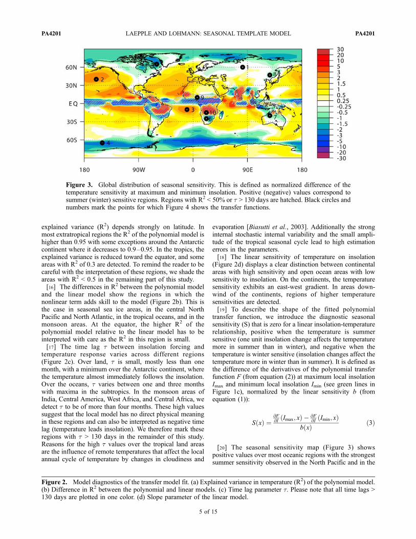
[20] The seasonal sensitivity map (Figure 3) showspositive values over most oceanic regions with the strongestsummer sensitivity observed in the North Pacific and in the

Figure 3. Global distribution of seasonal sensitivity. This is defined as normalized difference of thetemperature sensitivity at maximum and minimum insolation. Positive (negative) values correspond tosummer (winter) sensitive regions. Regions with R2 < 50% or t > 130 days are hatched. Black circles andnumbers mark the points for which Figure 4 shows the transfer functions.

Figure 2. Model diagnostics of the transfer model fit. (a) Explained variance in temperature (R2) of the polynomial model.(b) Difference in R2 between the polynomial and linear models. (c) Time lag parameter t. Please note that all time lags >130 days are plotted in one color. (d) Slope parameter of the linear model.


5 of 15

PA4201

subtropical oceans. In polar latitudes, the Arctic and theAntarctic sea ice regions are winter sensitive. The temper-ature over the midlatitude continents behaves linearly. In thetropics, the structure is more complicated as stronglysummer sensitive as well as winter sensitive regions aredetected. However, these regions also have a low R2 and/ora negative time lag.[21] We propose a qualitative classification of the

regionally different response functions to several responseregimes. These are based upon the shape of the transferfunction and are exemplified by specific locations (Figure 4).

[22] 1. Over extratropical continental areas, the responsefunction is close to linear [Huybers, 2006]. One example isCentral Asia (Figure 4, transfer function 1).[23] 2. Enhanced mixing of the ocean surface layer in

local winter and related changes in seasonal mixed layerdepth (MLD), defined as depth with nearly uniformtemperature, lead to a stronger damping of the wintertemperature response in the midlatitude and subtropicaloceans. A qualitative attribution of the summer sensitivityto MLD changes can be made by comparing the patternsto a seasonal MLD climatology [Kara et al., 2003].Examples for this regime are areas in the North Pacific

Figure 4. Seasonal cycles and transfer functions for selected points which are marked in Figure 3. Meanseasonal temperature cycle (black), the seasonal cycle as predicted by a linear model (red dashed) and apolynomial model (blue). The linear model (red) and polynomial model (blue) are shown along with thetemperature (black circles).


6 of 15

PA4201

(Figure 4, transfer function 2) and southern tropical Atlantic(Figure 4, transfer function 3). In the seasonal cycles, thesummer sensitivity is detected as narrow summers andbroad winters.[24] 3. Regions with seasonal sea ice cover [Rayner et al.,

2003] are more sensitive to winter insolation. In winter, thesea ice cover insulates the warmer ocean from the atmo-sphere, providing an additional cooling [e.g., Jackson andBroccoli, 2003]. This applies around Antarctica (Figure 4,transfer function 4) as well as at the arctic sea ice boundary(Figure 4, transfer function 5). In the response function, thisis detected as a division into a summer part with a smallinsolation-temperature slope and a winter part with a largeslope.[25] 4. Our transfer function shows a winter sensitivity in

regions which are classical monsoon areas [e.g., Lau et al.,2007]. These regional climates are characterized by asummer precipitation maximum driven by seasonal winds.The summer precipitation leads to evaporative cooling ofthe surface temperature and acts as a negative feedbackwhen we regard the temperature as function of localinsolation. Examples are South Africa (Figure 4, transferfunction 6), North Australia (Figure 4, transfer function 7)and East Asia (Figure 4, transfer function 8). The seasonalcycles are characterized by broad summers, whichare represented by a small summer slope in the transferfunctions.[26] 5. In some regions in the tropics, including the Asian

and African monsoon, the local polynomial model cannotwell explain the seasonal cycle [Biasutti et al., 2003].Examples are shown for West Africa (Figure 4, transferfunction 9) and Central Africa (Figure 4, transfer function10). We still apply our polynomial model which leads to astrongly nonlinear response. A similar nonlocality can befound in ocean regions around the equator. In these regions,nonlocal effects like coastal upwelling modulated by along-shore winds and changes in heat loss due to annualvariations in wind speed have a strong effect [Carton andZhou, 1997].

3.2. Application to the Mid-Holocene

[27] As a test of our concept, we predict the surfacetemperature trends between the mid-Holocene (7 ka) andpreindustrial (PI) conditions by applying the linear andpolynomial transfer functions on the historical insolationover the last 7 ka. The results are compared to transientsimulations of the coupled AOGCM ECHO-G [Lorenz andLohmann, 2004].[28] The surface temperature trend in annual mean tem-

peratures, predicted assuming a linear response to insolationforcing, shows a weak tripole pattern (Figure 5a). A coolingtrend from the mid-Holocene to PI in the polar latitudesnorth of 60�N and south of 60�S of up to 0.5�C/7 ka and aslight warming trend of less than 0.1�C/7 ka in tropical landareas are found. Using the polynomial transfer function, thetemperature trend pattern is more complex and the trendsare stronger (Figure 5b). The large-scale patterns are acooling trend at high latitudes and a dipole pattern in thetropics/midlatitudes, consisting of a cooling trend in the

Northern Hemisphere and a warming trend in the SouthernHemisphere.[29] The temperature trend pattern as simulated by the

ECHO-G climate model (Figure 5c) has a strong similaritywith the patterns of the polynomial template model. Again acooling trend in the high latitudes and a dipole pattern in themidlatitudes (cooling in the Northern Hemisphere, warmingin the Southern Hemisphere) are found. Regional warmingin the Sahel, South Asia, and the east coast of China and acooling trend inNorthAustralia, SouthAfrica, andMadagascarare detected, in line with the polynomial model.[30] Remarkably, signatures of all the response regimes

that we discussed for the present-day temperature cycle aredetected in the Holocene temperature trends in the data-based polynomial model as well as in the ECHO-G simu-lation. Regions in the Northern Hemisphere that showsummer sensitivity in the present-day seasonal cycle showa cooling trend and winter sensitive regions a warmingtrend. In the Southern Hemisphere, the relationship isinverted. In the polynomial model, temperatures in theseasonal mixing regime show a cooling trend of up to1�C in the Northern Hemisphere, for example in the NorthPacific. In the Southern Hemisphere, the correspondingwarming trend is 0.2–0.5�C. Similar patterns are found inthe GCM simulation, but details in the spatial extent andstrength of the trend differ from the polynomial model.[31] The predictions of the polynomial template model for

regions with seasonal sea ice cover are too warm in theNorthern Hemisphere and too cool in the Southern Hemi-sphere compared to the GCM results. Reasons for thismismatch in polar latitudes are changes in the mean seaice cover in the GCM simulation (hatched areas inFigure 5c) that strongly affect the surface temperature. Thisleads to strong cooling trends in most sea ice areas in theGCM simulations except in some patches in the SouthernHemisphere at 100�Wand 25�W that show a decrease in seaice cover and therefore a warming trend in the GCM. Asimilar mechanism can explain the differences in the tem-perature trend between the ECHO-G simulations and thetemplate model over Europe and central North America.The present-day seasonal snow cover leads to a slight wintersensitivity (see Figure 3), and therefore a warming trend inthe template model predictions. In ECHO-G, the mean snowcover shows a positive trend which leads to a cooling. Sincethe mid-Holocene, precipitation in the monsoon areas hasdecreased in the Northern Hemisphere and increased in theSouthern Hemisphere [Liu et al., 2004]. This lead to awarming trend in the Northern Hemisphere regions and acooling trend in the Southern Hemisphere regions. Thesechanges are reproduced by the ECHO-G model as well aswith the polynomial model in all monsoon regions (SouthAfrica, North Australia, East Asia, and West Africa) exceptthe Indian monsoon region where the polynomial modelpredicts a trend in the wrong direction. A reduction inmonsoon precipitation in Mexico [Liu et al., 2004] leads toa warming trend in the GCM simulation which is notcaptured by the polynomial model. Moreover, changes inthe atmospheric circulation as well as climate feedbackssimulated by the GCM are not included in our data-basedapproach. Such feedbacks are likely responsible for the


7 of 15

PA4201

mismatch between both approaches in the North Atlantic. Inthis region, the GCM simulates a change in the mean stateof the North Atlantic oscillation (NAO) and associatedhigh-latitude temperature and sea ice changes [Lorenz andLohmann, 2004; Lohmann et al., 2005].

3.3. Impact on Long-Term Variability

[32] As a further application of our linear and polynomialmodel, we examine the temperature evolution of the last750 ka. The results are analyzed in the spectral domain byusing the periodogram of the time series [Bloomfield, 1976].

Figure 5. Temperature trend between the mid-Holocene (7 ka) and PI (0 ka) in �C/7 ka. (a) As predictedby the linear model, (b) as predicted by the polynomial model, and (c) from the ECHO-G AOGCMsimulation [Lorenz et al., 2006]. In Figure 5b regions with R2 < 50% or t > 130 days are hatched. InFigure 5c regions with a sea ice trend > 3%/ka corresponding to a 0.5–1�C/7 ka temperature trend,assuming a sea ice temperature of �15 to �30�C, are hatched.


8 of 15

PA4201

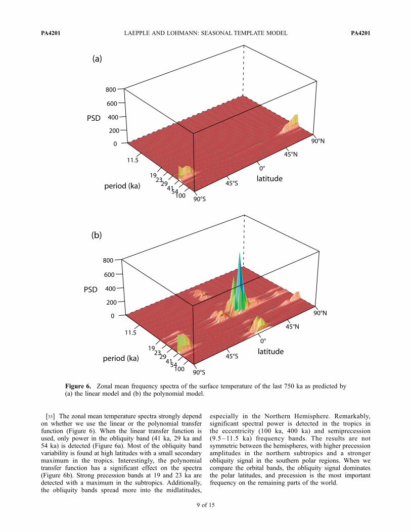
[33] The zonal mean temperature spectra strongly dependon whether we use the linear or the polynomial transferfunction (Figure 6). When the linear transfer function isused, only power in the obliquity band (41 ka, 29 ka and54 ka) is detected (Figure 6a). Most of the obliquity bandvariability is found at high latitudes with a small secondarymaximum in the tropics. Interestingly, the polynomialtransfer function has a significant effect on the spectra(Figure 6b). Strong precession bands at 19 and 23 ka aredetected with a maximum in the subtropics. Additionally,the obliquity bands spread more into the midlatitudes,

especially in the Northern Hemisphere. Remarkably,significant spectral power is detected in the tropics inthe eccentricity (100 ka, 400 ka) and semiprecession(9.5–11.5 ka) frequency bands. The results are notsymmetric between the hemispheres, with higher precessionamplitudes in the northern subtropics and a strongerobliquity signal in the southern polar regions. When wecompare the orbital bands, the obliquity signal dominatesthe polar latitudes, and precession is the most importantfrequency on the remaining parts of the world.

Figure 6. Zonal mean frequency spectra of the surface temperature of the last 750 ka as predicted by(a) the linear model and (b) the polynomial model.


9 of 15

PA4201

Figure 7


10 of 15

PA4201

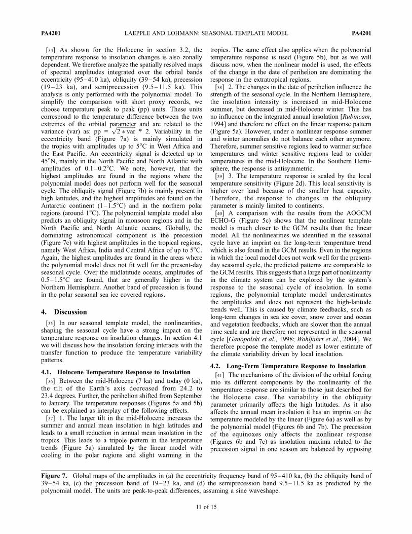
[34] As shown for the Holocene in section 3.2, thetemperature response to insolation changes is also zonallydependent. We therefore analyze the spatially resolved mapsof spectral amplitudes integrated over the orbital bandseccentricity (95–410 ka), obliquity (39–54 ka), precession(19–23 ka), and semiprecession (9.5–11.5 ka). Thisanalysis is only performed with the polynomial model. Tosimplify the comparison with short proxy records, wechoose temperature peak to peak (pp) units. These unitscorrespond to the temperature difference between the twoextremes of the orbital parameter and are related to thevariance (var) as: pp =

ffiffiffiffiffiffiffiffiffiffiffiffiffiffi

2 � varp

* 2. Variability in theeccentricity band (Figure 7a) is mainly simulated inthe tropics with amplitudes up to 5�C in West Africa andthe East Pacific. An eccentricity signal is detected up to45�N, mainly in the North Pacific and North Atlantic withamplitudes of 0.1–0.2�C. We note, however, that thehighest amplitudes are found in the regions where thepolynomial model does not perform well for the seasonalcycle. The obliquity signal (Figure 7b) is mainly present inhigh latitudes, and the highest amplitudes are found on theAntarctic continent (1–1.5�C) and in the northern polarregions (around 1�C). The polynomial template model alsopredicts an obliquity signal in monsoon regions and in theNorth Pacific and North Atlantic oceans. Globally, thedominating astronomical component is the precession(Figure 7c) with highest amplitudes in the tropical regions,namely West Africa, India and Central Africa of up to 5�C.Again, the highest amplitudes are found in the areas wherethe polynomial model does not fit well for the present-dayseasonal cycle. Over the midlatitude oceans, amplitudes of0.5–1.5�C are found, that are generally higher in theNorthern Hemisphere. Another band of precession is foundin the polar seasonal sea ice covered regions.

4. Discussion

[35] In our seasonal template model, the nonlinearities,shaping the seasonal cycle have a strong impact on thetemperature response on insolation changes. In section 4.1we will discuss how the insolation forcing interacts with thetransfer function to produce the temperature variabilitypatterns.

4.1. Holocene Temperature Response to Insolation

[36] Between the mid-Holocene (7 ka) and today (0 ka),the tilt of the Earth’s axis decreased from 24.2 to23.4 degrees. Further, the perihelion shifted from Septemberto January. The temperature responses (Figures 5a and 5b)can be explained as interplay of the following effects.[37] 1. The larger tilt in the mid-Holocene increases the

summer and annual mean insolation in high latitudes andleads to a small reduction in annual mean insolation in thetropics. This leads to a tripole pattern in the temperaturetrends (Figure 5a) simulated by the linear model withcooling in the polar regions and slight warming in the

tropics. The same effect also applies when the polynomialtemperature response is used (Figure 5b), but as we willdiscuss now, when the nonlinear model is used, the effectsof the change in the date of perihelion are dominating theresponse in the extratropical regions.[38] 2. The changes in the date of perihelion influence the

strength of the seasonal cycle. In the Northern Hemisphere,the insolation intensity is increased in mid-Holocenesummer, but decreased in mid-Holocene winter. This hasno influence on the integrated annual insolation [Rubincam,1994] and therefore no effect on the linear response pattern(Figure 5a). However, under a nonlinear response summerand winter anomalies do not balance each other anymore.Therefore, summer sensitive regions lead to warmer surfacetemperatures and winter sensitive regions lead to coldertemperatures in the mid-Holocene. In the Southern Hemi-sphere, the response is antisymmetric.[39] 3. The temperature response is scaled by the local

temperature sensitivity (Figure 2d). This local sensitivity ishigher over land because of the smaller heat capacity.Therefore, the response to changes in the obliquityparameter is mainly limited to continents.[40] A comparison with the results from the AOGCM

ECHO-G (Figure 5c) shows that the nonlinear templatemodel is much closer to the GCM results than the linearmodel. All the nonlinearities we identified in the seasonalcycle have an imprint on the long-term temperature trendwhich is also found in the GCM results. Even in the regionsin which the local model does not work well for the present-day seasonal cycle, the predicted patterns are comparable tothe GCM results. This suggests that a large part of nonlinearityin the climate system can be explored by the system’sresponse to the seasonal cycle of insolation. In someregions, the polynomial template model underestimatesthe amplitudes and does not represent the high-latitudetrends well. This is caused by climate feedbacks, such aslong-term changes in sea ice cover, snow cover and oceanand vegetation feedbacks, which are slower than the annualtime scale and are therefore not represented in the seasonalcycle [Ganopolski et al., 1998; Wohlfahrt et al., 2004]. Wetherefore propose the template model as lower estimate ofthe climate variability driven by local insolation.

4.2. Long-Term Temperature Response to Insolation

[41] The mechanisms of the division of the orbital forcinginto its different components by the nonlinearity of thetemperature response are similar to those just described forthe Holocene case. The variability in the obliquityparameter primarily affects the high latitudes. As it alsoaffects the annual mean insolation it has an imprint on thetemperature modeled by the linear (Figure 6a) as well as bythe polynomial model (Figures 6b and 7b). The precessionof the equinoxes only affects the nonlinear response(Figures 6b and 7c) as insolation maxima related to theprecession signal in one season are balanced by opposing

Figure 7. Global maps of the amplitudes in (a) the eccentricity frequency band of 95–410 ka, (b) the obliquity band of39–54 ka, (c) the precession band of 19–23 ka, and (d) the semiprecession band 9.5–11.5 ka as predicted by thepolynomial model. The units are peak-to-peak differences, assuming a sine waveshape.


11 of 15

PA4201

insolation minima in the opposite season. The amplitude ofthe simulated precession signal is a convolution of theamplitude of the forcing, which is strongest in the subtropics,the degree of nonlinearity (generally higher and tropics) andthe temperature sensitivity (highest over land).[42] The shape of the nonlinear response (higher temper-

ature sensitivity in summer or in winter) determines thephase of the precession signal. This is detected in theHolocene analysis where some regions show a coolingtrend whereas other regions show a warming trend(Figure 5b). It is also demonstrated by contrasting timeseries, simulated by the polynomial model, for summerand winter sensitive regions of the same hemisphere. Figure 8shows a typical example, the temperature time series of NorthAustralia and the Indian Ocean, simulated by the polynomialmodel. Both show a strong precession signal, but the phasesof the precession signal oppose each other although theyare forced by the same insolation variability. This phasedependency of the temperature signal on the seasonal sensi-tivity leads to the intriguing situation that a winter sensitivearea in the Southern Hemisphere will perfectly correlate withNorthern Hemispheric summer insolation, although drivenby local insolation. A similar idea has been proposedfor Antarctica by Stott et al. [2007], who suggest that seaice leads to a spring sensitive temperature response andby Huybers and Denton [2008] who propose that the non-linearity of the radiative balance leads to a locally forcedprecession signal in the Antarctic temperature.[43] Changes in eccentricity of the Earth’s orbit have a

small effect on global mean insolation but modulate theamplitude of the precession. A strongly nonlinear temper-ature response such as in the North Pacific demodulates theeccentricity signal (Figure 7a). In intertropical regions,the Sun comes overhead twice a year at each latitude. Inthe case of a nonlinear transfer function one of the twoinsolation maxima gets favored regardless of the time whenthey occur in the year. As the insolation at spring andautumn equinoxes is out of phase by a half-precessioncycle, this leads to the power in the semiprecession bandand the eccentricity band (Figures 7a and 7d) [Ashkenazyand Gildor, 2008]. This partitioning of the forcing in the

intertropical band into eccentricity and semiprecession wasalso found by Crowley et al. [1992] who prescribed athreshold response function to explain the spectra foundin Triassic lake deposits. Berger and Loutre [1997] andBerger et al. [2006] used the maximum insolation during ayear as metric to demonstrate that half-precession cycles canbe generated from orbital forcing. In contrast to thesestudies that are based on ad hoc transfer functions, ourmodel shows that the observed present-day transfer functioncan already explain these frequencies.[44] Other tools to investigate the problem of the long-

term climate response to insolation are Energy BalanceModels (EBM). The pioneering work using this techniqueis that by Short et al. [1991] who used a linear, two-dimensional, seasonal EBM to study the spatial pattern ofthe temperature response to long-term insolation. Theirresults for the annual mean temperature response [e.g.,Short et al., 1991, Figure 9] are similar to our results fromthe linear model showing only variability in the obliquityband. Short et al. [1991] further analyzed the maximumseasonal temperature as diagnostics to obtain a temperatureresponse comparable to the response found in proxyrecords. In our polynomial template approach, we do notneed this assumption and see that the nonlinearities alreadypresent in the seasonal cycle lead to a realistic response ofthe annual mean temperature.[45] Our concept is related to two recent hypotheses

concerning the climate response to insolation variations.The summer energy concept [Huybers, 2006; Huybers andTziperman, 2008] provides an explanation for the glacialcycles of the early Pleistocene by proposing that glaciers aresensitive to the integrated summer insolation. This conceptis based on the approximation of the annual ablation bypositive degree days and the assumption of a linearrelationship between temperature and insolation whichcollaborates with our findings of a linear relationship onextratropical land regions. The integrated summer energyconcept and our model address different questions andcomplement each other. The summer energy model simu-lates the annual ablation and therefore the response of theglacial mass balance to insolation changes. This question

Figure 8. Temperature time series of the last 200 ka as predicted by the polynomial model. NorthAustralia (20�S, 135�E) (black) and Indian Ocean (20�S, 100�E) (red dashed).


12 of 15

PA4201

cannot be addressed by the seasonal template model aschanges in the glacial mass balance and their influence ontemperature are slow processes not captured in the modernseasonal cycle of temperature. The summer energy concepton the other hand is limited to a specific nonlinear physicalmechanism, the ablation. It is therefore not able to resolveother climate feedbacks like the mixed layer depth ormonsoon regimes that play an important role in shapingthe regional temperature response to insolation.[46] Recently Huybers and Denton [2008] addressed the

question of the temperature variability on orbital timescalesin Antarctica, proposing that the Antarctic temperature isdetermined by the local summer duration and not by thesummer insolation intensity. The basis for this hypothesis isthat the radiative balance indicates greater temperaturesensitivity at lower temperatures. This directly relates tothe work presented in this paper as a lower sensitivity onwarmer temperatures should be detectable in the modernseasonal cycle of temperature. In Antarctica, our analysissuggests a linear or summer sensitive temperature response(section 3.1 and Figure 3) and does therefore not support thesummer length hypothesis. More work is needed to under-stand the reasons and the significance of the discrepanciesbetween the empirical transfer function of insolation andtemperature (this study) and the summer length hypothesis[Huybers and Denton, 2008]. Potential candidates for thedifferences include problems with the NCEP reanalysis inAntarctica [Hines et al., 1999] that may lead to artificialsummer sensitivity in our study as well as influences onseasonal energy balance in Antarctica, not considered in thesummer length hypothesis, which mask or even invert thehigher sensitivity to low temperatures given by the radiativebalance.

4.3. Limitations of the Concept

[47] The two basic assumptions of our model (timeindependence and locality) lead to certain limitations. Theclimate response is time-dependent, and therefore not allfeedback processes are captured in our data source, theseasonal cycle. Slow processes like the evolution of icesheets or changes in the ocean circulation will therefore addmore nonlinearities to the system than included by ourseasonal template. Furthermore, the boundary conditionswhich determine the seasonal climate response, and there-fore our template, are changing with time. One example isthe variation in the sea ice covered area that modifies theposition and extent of the winter sensitive regime. Thisleads to misfits between our data-based model and GCMresults in the polar latitudes (Figures 5b and 5c).[48] The climate system is characterized by pronounced

spatial correlations (teleconnections) caused by atmospheric[e.g., Rimbu et al., 2003; Rodgers et al., 2003; Wallace andGutzler, 1981] and ocean dynamics. As the insolationforcing is similar over wide areas, some nonlocal effectsare captured by our local approach, but large-scaleteleconnections as the NAO cause a misfit of our data-based model in some regions (e.g., Figures 5b and 5c, NorthAtlantic Region). On long time scales, the large-scale oceancirculation [Stocker, 1998] as well as greenhouse gases leadto interhemispheric coupling.

[49] For the comparison of our model predictions withproxy records, one further has to consider that our resultsare the predicted frequency spectra of the physical quantitytemperature. In paleorecords, one might expect alteredspectra caused by the additional nonlinearity added by therecorder system [Crowley et al., 1992; Huybers andWunsch, 2003].

5. Conclusions

[50] We propose a simple model for insolation-drivenclimate variability on astronomical timescales. Under theassumption that the climate response to insolation is thesame on seasonal as well as on astronomical timescales weuse the observed seasonal cycle of temperature to derive thespatially resolved surface temperature variability of the last750 ka. Our results show that nonlinearities and feedbacksrepresented in the observed present-day seasonal cycle havelarge effects on the long-term climate variability. As oneexample for the interglacial climate evolution we study theHolocene temperature trends by comparing a linear templatemodel, a nonlinear template model, and a simulation of acomplex AOGCM. This model hierarchy allows us todistinguish between linear effects, feedbacks that happenon a seasonal time scale, and long-term feedbacks. Thetemplate model therefore acts as a tool for the interpretationof complex model simulations.[51] Our results have the following implications for the

interpretation of paleorecords.[52] 1. Even at one latitude, different frequency spectra of

the temperature evolution are expected, e.g., variability inthe obliquity band can dominate in one region whereasvariability in the precession band can dominate in anotherregion.[53] 2. The phase of the astronomically induced temper-

ature changes can vary, depending on the nonlinearity.Regions with a seasonal cycle sensitive to winter insolation(e.g., North Australia) will show a precession signal with aphase opposite to that of summer sensitive areas (Figure 8).This leads to the intriguing situation that a winter sensitivearea in the Southern Hemisphere will perfectly correlatewith Northern Hemispheric summer insolation, even if it isdriven by local insolation.[54] 3. In tropical areas, a temperature signal in the

eccentricity band as well as in the semiprecession band ispredicted with significant amplitude. This corresponds wellwith results from Crowley et al. [1992], Berger and Loutre[1997], and Berger et al. [2006] with the difference that wedid not have to prescribe a specific transfer function. Thesimultaneous appearance of semiprecession and eccentricitywhich is found in paleodata [Rutherford and D’Hondt,2000] can be directly explained by a nonlinear responseto the local insolation.[55] 4. The land-sea pattern modulates the amplitude of

the temperature response. This corresponds well with theresults found by Short et al. [1991], who used an EBM tostudy the temperature response on orbital forcing. For theannual mean temperatures, we observe two competingeffects: The larger heat capacity of the ocean damps thetemperature response, but the generally higher nonlinearity


13 of 15

PA4201

over the ocean amplifies the response on the precessionforcing. The obliquity response is generally stronger overland, but the precession response does not show a clearocean/land classification.[56] On the basis of the comparison to a Holocene GCM

experiment [Lorenz et al., 2006; Lorenz and Lohmann,2004], we propose our result as lower estimate of theregional effects of insolation. Large-scale changes likethe buildup and retreat of ice sheets and their effect onthe global mean temperature add up to these effects. In thisway, our model can be seen as a complementary concept tothe common approach of relating climate records from allover the world to 65�N summer insolation. It remains openwhether the local effects we found may influence the globalscale. The tropical temperature variability that we found inthe eccentricity and semiprecession band might act on thehigh-latitude climate via teleconnections [e.g., Cane, 1998;Huybers and Molnar, 2007; Rodgers et al., 2003]. Thisinterplay of local and global effects remains open for furtherstudies.[57] Our results are also a reminder to be careful in using

orbital tuning to date paleorecords. The amplitudes that ourmodel predicts for the temperature response on local

insolation have a magnitude similar to that of reconstructedglacial-interglacial changes in tropical and subtropicallatitudes [Farrera et al., 1999; Pflaumann et al., 2003].This implies that the surface temperatures and relatedclimate variables are not globally correlative, and evenspatially close records may differ in their phasing.Therefore, using some ad hoc tuning target as the 65�Nsummer insolation to determine the time scale of proxyrecords might not be justified.[58] The method of using the seasonal cycle as template

can also be applied for other variables, such as precipitationor dust. Here a locally measured seasonal cycle can beused to predict the local response to orbital insolationchanges and give a starting point for the interpretation ofpaleorecords.

[59] Acknowledgments. This study was funded by the HelmholtzAssociation through the programs MARCOPOLI and PACES. We wouldlike to thank Andrea Bleyer for her help in preparing this manuscript. Thispaper benefited from discussions with Frank Lamy and Klaus Grosfeld. Weare grateful to the reviewers Lorraine E. Lisiecki and Peter Huybers, as wellas to Gerald Dickens, for their detailed comments on the manuscript.

ReferencesAdhemar, J. (1842), Revolutions de la Mer,Carilian-Goeury et V. Dalmont, Paris.

Ashkenazy, Y., and H. Gildor (2008), Timingandsignificanceofmaximumandminimumequatorialinsolation, Paleoceanography, 23, PA1206,doi:10.1029/2007PA001436.

Berger, A. L. (1978), Long-term variations ofdaily insolation and quaternary climaticchanges, J. Atmos. Sci., 35(12), 2362–2367,d o i : 1 0 . 11 7 5 / 1 5 20 - 0 4 69 ( 1 9 78 ) 0 3 5<2362:LTVODI>2.0.CO;2.

Berger, A., andM. Loutre (1991), Insolation valuesfor the climate of the last 10 million years,Quat.Sci. Rev., 10(4), 297–317, doi:10.1016/0277-3791(91)90033-Q.

Berger, A., and M. F. Loutre (1997), Intertropicallatitudes and precessional and half-precessionalcycles, Science, 278(5342), 1476 – 1478,doi:10.1126/science.278.5342.1476.

Berger, A., M. F. Loutre, and J. L. Melice (2006),Equatorial insolation:Fromprecessionharmonicsto eccentricity frequencies, Clim. Past, 2(2),131–136.

Biasutti, M., D. S. Battisti, and E. S. Sarachik(2003), The annual cycle over the tropicalAtlantic, South America, and Africa, J. Clim.,16(15), 2491 – 2508, doi:10.1175/1520-0442(2003)016<2491:TACOTT>2.0.CO;2.

Bloomfield, P. (1976), Fourier Analysis of TimeSeries: An Introduction, JohnWiley, NewYork.

Broecker, W. S., and J. van Donk (1970), Insola-tion changes, ice volumes, and the O18 recordin deep-sea cores, Rev. Geophys., 8, 169–198,doi:10.1029/RG008i001p00169.

Cane, M. A. (1998), Climate change: A role forthe tropical Pacific, Science, 282(5386), 59–61,doi:10.1126/science.282.5386.59.

Carton, J. A., and Z. Zhou (1997), Annual cycleof sea surface temperature in the tropicalAtlantic Ocean, J. Geophys. Res., 102(C13),27,813–27,824, doi:10.1029/97JC02197.

Clemens, S., W. Prell, D. Murray, G. Shimmield,and G. Weedon (1991), Forcing mechanismsof the Indian Ocean monsoon, Nature ,353(6346), 720–725, doi:10.1038/353720a0.

Clement, A. C., A. Hall, and A. J. Broccoli(2004), The importance of precessional signalsin the tropical climate, Clim. Dyn., 22(4),327–341, doi:10.1007/s00382-003-0375-8.

Croll, J. (1875), Climate and Time in TheirGeological Relations: A Theory of SecularChanges of the Earth’s Climate, DaldyTsbister, London.

Crowley, T. J., K. Y. Kim, J. G. Mengel, andD. A. Short (1992), Modeling 100,000-yearclimate fluctuations in pre-Pleistocene time-series, Science , 255(5045), 705 – 707,doi:10.1126/science.255.5045.705.

Farrera, I., et al. (1999),Tropical climates at theLastGlacial Maximum: A new synthesis of terrestrialpalaeoclimate data. I. Vegetation, lake-levels andgeochemistry, Clim. Dyn., 15(11), 823–856,doi:10.1007/s003820050317.

Ganopolski, A., C. Kubatzki, M. Claussen,V. Brovkin, and V. Petoukhov (1998), Theinfluence of vegetation-atmosphere-oceaninteraction on climate during themid-Holocene,Science, 280(5371), 1916–1919, doi:10.1126/science.280.5371.1916.

Hays, J. D., J. Imbrie, andN. J. Shackleton (1976),Variations in the Earth’s orbit: Pacemaker of theice ages, Science, 194(4270), 1121 – 1132,doi:10.1126/science.194.4270.1121.

Held, I. (2005), The gap between simulation andunderstanding in climate modeling, Bull. Am.Meteoro l . Soc . , 86 (11) , 1609 – 1614,doi:10.1175/BAMS-86-11-1609.

Hines, K. M., R. W. Grumbine, D. H. Bromwich,and R. I. Cullather (1999), Surface energybalance of the NCEP MRF and NCEP-NCARreanalysis in Antarctic latitudes duringFROST, Weather Forecasting, 14(6), 851–866, doi:10.1175/1520-0434(1999)014<0851:SEBOTN>2.0.CO;2.

Huybers, P. (2006), Early Pleistocene glacialcycles and the integrated summer insolationforcing, Science , 313(5786), 508 – 511,doi:10.1126/science.1125249.

Huybers, P., and G. Denton (2008), Antarctictemperature at orbital timescales controlled

by local summer duration, Nat. Geosci.,1(11), 787–792, doi:10.1038/ngeo311.

Huybers, P., and P. Molnar (2007), Tropical cool-ing and the onset of North American glaciation,Clim. Past, 3(3), 549–557.

Huybers, P., and E. Tziperman (2008), Integratedsummer insolation forcing and 40,000-year gla-cial cycles: The perspective from an ice-sheet/energy-balance model, Paleoceanography, 23,PA1208, doi:10.1029/2007PA001463.

Huybers, P., and C. Wunsch (2003), Rectificationand precession signals in the climate system,Geophy s . Re s . L e t t . , 30 ( 19 ) , 2011 ,doi:10.1029/2003GL017875.

Imbrie, J., et al. (1992), On the structure andorigin of major glaciation cycles: 1. Linearresponses to Milankovitch forcing, Paleoceano-graphy, 7, 701–738, doi:10.1029/92PA02253.

Jackson, C. S., and A. J. Broccoli (2003), Orbitalforcing of Arctic climate: Mechanisms ofclimate response and implications for continentalglaciation, Clim. Dyn., 21(7 – 8), 539 –557,doi:10.1007/s00382-003-0351-3.

Kalnay, E., et al. (1996), TheNCEP/NCAR40-yearreanalysis project, Bull. Am. Meteorol. Soc.,77 ( 3 ) , 437 – 471 , do i : 10 .1175 / 1520 -0477(1996)077<0437:TNYRP>2.0.CO;2.

Kara, A. B., P. A. Rochford, and H. E. Hurlburt(2003), Mixed layer depth variability over theglobal ocean, J. Geophys. Res., 108(C3), 3079,doi:10.1029/2000JC000736.

Laskar, J., P. Robutel, F. Joutel, M. Gastineau,A. C. M. Correia, and B. Levrard (2004), Along-term numerical solution for the insolationquantities of the Earth, Astron. Astrophys.,428(1), 261 – 285, doi:10.1051/0004-6361:20041335.

Lau, W. K. M., K. M. Kim, and M. I. Lee (2007),Characteristics of diurnal and seasonal cycles inglobalmonsoon systems, J.Meteorol. Soc. Jpn.,85A, 403–416, doi:10.2151/jmsj.85A.403.

Liu, Z., S. P. Harrison, J. Kutzbach, andB. Otto-Bliesner (2004), Global monsoons inthe mid-Holocene and oceanic feedback, Clim.Dyn., 22(2–3), 157–182.


14 of 15

PA4201

Lohmann, G., S. J. Lorenz, and M. Prange(2005), Northern high-latitude climate changesduring the Holocene as simulated by circula-tion models, in The Nordic Seas: An IntegratedPerspective—Oceanography, Climatology,Biogeochemistry, and Modeling, Geophys.Monogr. Ser., vol. 158, edited by H. Drangeet al., pp. 273–288, AGU, Washington, D. C.

Lorenz, S. J., and G. Lohmann (2004), Accelera-tion technique for Milankovitch type forcing ina coupled atmosphere-ocean circulationmodel: Method and application for theHolocene, Clim. Dyn., 23(7 – 8), 727 –743,doi:10.1007/s00382-004-0469-y.

Lorenz, S. J., J.-H. Kim, N. Rimbu, R. R.Schneider, and G. Lohmann (2006), Orbitallydriven insolation forcing on Holocene climatetrends: Evidence from alkenone data andclimate modeling, Paleoceanography, 21,PA1002, doi:10.1029/2005PA001152.

Loutre, M. F., D. Paillard, F. Vimeux, andE. Cortijo (2004), Does mean annual insolationhave the potential to change the climate?, EarthP lane t . Sc i . Le t t . , 221 ( 1 – 4 ) , 1 – 14 ,doi:10.1016/S0012-821X(04)00108-6.

Milankovitch, M. (1941), Kanon der Erdbestrah-lung und Seine Anwendung auf das Eiszeiten-problem, vol. 133, 633 pp., Akad. R. Serbia,Belgrade.

Pahnke, K., and J. P. Sachs (2006), Sea surfacetemperatures of southern midlatitudes 0 –160 kyr B.P., Paleoceanography, 21 ,PA2003, doi:10.1029/2005PA001191.

Pahnke, K., R. Zahn, H. Elderfield, andM. Schulz(2003), 340,000-year centennial-scale marine

record of Southern Hemisphere climatic oscilla-tion, Science, 301(5635), 948–952.

Pflaumann, U., et al. (2003), Glacial NorthAtlantic: Sea-surface conditions reconstructedby GLAMAP 2000, Paleoceanography, 18(3),1065, doi:10.1029/2002PA000774.

Rayner, N. A., D. E. Parker, E. B. Horton, C. K.Folland, L. V. Alexander, D. P. Rowell, E. C.Kent, and A. Kaplan (2003), Global analysesof sea surface temperature, sea ice, and nightmarine air temperature since the late nineteenthcentury, J. Geophys. Res., 108(D14), 4407,doi:10.1029/2002JD002670.

Rimbu, N., G. Lohmann, J.-H. Kim, H. W. Arz,and R. Schneider (2003), Arctic/North AtlanticOscillation signature in Holocene sea surfacetemperature trends as obtained from alkenonedata, Geophys. Res. Lett., 30(6), 1280,doi:10.1029/2002GL016570.

Rodgers, K. B., G. Lohmann, S. Lorenz,R. Schneider, and G. M. Henderson (2003), Atropical mechanism for Northern Hemispheredeglaciation, Geochem. Geophys. Geosyst.,4(5), 1046, doi:10.1029/2003GC000508.

Rubincam, D. P. (1994), Insolation in terms ofEarth’s orbital parameters, Theor. Appl. Climatol.,48(4), 195–202, doi:10.1007/BF00867049.

Rutherford, S., and S. D’Hondt (2000), Earlyonset and tropical forcing of 100,000-yearPleistocene glacial cycles, Nature, 408(6808),72–75, doi:10.1038/35040533.

Short, D. A., J. G. Mengel, T. J. Crowley, W. T.Hyde, and G. R. North (1991), Filtering ofMilankovitch cycles by Earth’s geography,

Quat. Res., 35(2), 157 – 173, doi:10.1016/0033-5894(91)90064-C.

Stocker, T. F. (1998), Climate change: Theseesaw effect, Science, 282(5386), 61 – 62,doi:10.1126/science.282.5386.61.

Stott, L., A. Timmermann, and R. Thunell(2007), Southern Hemisphere and deep-seawarming led deglacial atmospheric CO2 riseand tropical warming, Science, 318(5849),435–438, doi:10.1126/science.1143791.

Tuenter, E., S. L. Weber, F. J. Hilgen, and L. J.Lourens (2003), The response of the Africansummer monsoon to remote and local forcingdue to precession and obliquity, Global Planet.Change, 36(4), 219–235, doi:10.1016/S0921-8181(02)00196-0.

Wallace, J. M., and D. S. Gutzler (1981),Teleconnections in the geopotential height fieldduring the Northern Hemisphere winter, Mon.Weather Rev., 109(4), 784–812, doi:10.1175/1520-0493(1981)109<0784:TITGHF>2.0.CO;2.

Wohlfahrt, J., S. P. Harrison, and P. Braconnot(2004), Synergistic feedbacks between oceanand vegetation on mid- and high-latitude climatesduring the mid-Holocene, Clim. Dyn., 22(2–3),223–238, doi:10.1007/s00382-003-0379-4.

��T. Laepple and G. Lohmann, Alfred Wegener

Institute for Polar andMarineResearch,Bussestrasse24, D-27570 Bremerhaven, Germany. ([email protected])


15 of 15

PA4201

Documents

Seasonal cycle as template for climate variability on