Seasonal circulation and temperature variability near the

Seasonal circulation and temperature variability near the NorthWest Cape of Australia

Ryan J. Lowe,1,2 Gregory N. Ivey,2,3 Richard M. Brinkman,4 and Nicole L. Jones2,3

Received 3 October 2011; revised 8 February 2012; accepted 17 February 2012; published 5 April 2012.

[1] The circulation and temperature variability on the inner shelf near the North West Capeof Australia off Ningaloo Reef was investigated using field data obtained from twomoorings deployed from 2004 to 2009. The results revealed that alongshore currents onthe inner shelf were, on average, only weakly influenced by the offshore poleward(southward) Leeuwin Current flow, i.e., monthly averaged alongshore current velocitieswere �0.1 m s�1 or less. The presence of a consistent summer-time wind-drivenequatorward (northward) counter flow on the inner-shelf (referred to in the literature as theNingaloo Current) was not observed. Instead, the shelf waters were strongly influencedyear-round by episodic subtidal current fluctuations (time scale 1–2 weeks) that were drivenby local wind-forcing. Analysis of the current profiles showed that periods of strongequatorward winds were able to overcome the dominant poleward pressure gradient in theregion, leading to upwelling on the inner-shelf. Contrary to prior belief, these events werenot limited to summer periods. The forcing provided by these periodic wind events andthe associated alongshore flows can explain much of the observed temperature variability(with timescales < 1 month) that influences Ningaloo Reef.

Citation: Lowe, R. J., G. N. Ivey, R. M. Brinkman, and N. L. Jones (2012), Seasonal circulation and temperature variability nearthe North West Cape of Australia, J. Geophys. Res., 117, C04010, doi:10.1029/2011JC007653.

1. Introduction

[2] Along the eastern margins of most ocean basins, theprevailing equatorward wind patterns at subtropical latitudesgenerate equatorward-flowing surface current systems thatdominate the continental shelf regions of these coastlines.These eastern boundary currents (for example, the California,Humboldt, Canary and Benguela Currents in the Pacific andAtlantic Oceans), promote coastal upwelling that supportsthe high rates of primary productivity observed in theseregions. However, off the coast of Western Australia (WA)in the southeast Indian Ocean, the surface circulation isdominated by the unique poleward-flowing (downwelling-favorable) Leeuwin Current (LC) [Cresswell and Golding,1980; Smith et al., 1991; Feng et al., 2003]. While equator-ward winds are also present along the coast of WA, thedominant forcing is provided by an anomalously largemeridional pressure gradient between the Australian NorthWest Shelf and the Southern Ocean, which is maintained bythe Indonesian Throughflow [Godfrey and Ridgway, 1985].The presence of the poleward flowing LC suppresses

persistent upwelling along the WA coast throughout most ofthe year, resulting in the sea surface temperature off WAbeing 4–5�C warmer than upwelling systems at similar sub-tropical latitudes [Feng and Wild-Allen, 2008]. As a result,the shelf waters off WA are considered oligotrophic, withprimary productivity rates generally < 200 mg C m�2 d�1

,

and thus much smaller than the typical > 1000 mg C m�2 d�1

observed in other eastern boundary current systems experi-encing persistent upwelling [Hanson et al., 2005].[3] Nevertheless, recent work off the coast of WA has

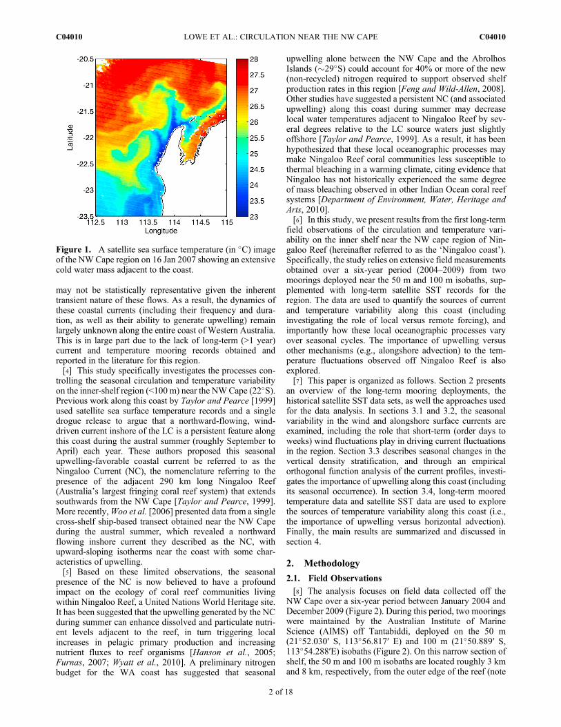
suggested that during summer months, when southerly windstresses are at their maximum, wind-driven northward(equatorward) counter-currents may form on the inner shelf,weakening and pushing the LC offshore [Gersbach et al.,1999; Woo et al., 2006]. These wind-driven coastal currentshave been proposed to generate episodic (transient) upwell-ing along some regions of WA where the continental shelf isrelatively narrow, such as between Cape Leeuwin and CapeNaturaliste near 34�S [Gersbach et al., 1999; Pearce andPattiaratchi, 1999], and along the North West Cape regionnear 22�S, the narrowest section of shelf anywhere inAustralia [Taylor and Pearce, 1999; Woo et al., 2006]. Onestriking example of a coastal cold water mass generated nearthe NW Cape in response to a period of strong southerlywinds in January 2007 is shown in Figure 1. Notably, allevidence used to examine these wind-driven coastal currentsand their potential for upwelling, have been derived fromeither: (1) historical satellite sea surface temperature (SST)imagery (as in Figure 1), which provides no direct insightinto the current or sub-surface density fields; or (2) a smallset of opportunistic ship-based hydrographic transects, which

1School of Earth and Environment, University of Western Australia,Crawley, Western Australia, Australia.

2Oceans Institute, University of Western Australia, Crawley, WesternAustralia, Australia.

3School of Environmental Systems Engineering, University of WesternAustralia, Crawley, Western Australia, Australia.

4Australian Institute of Marine Science, Townsville, Queensland,Australia.

Copyright 2012 by the American Geophysical Union.0148-0227/12/2011JC007653

JOURNAL OF GEOPHYSICAL RESEARCH, VOL. 117, C04010, doi:10.1029/2011JC007653, 2012

C04010 1 of 18

http://dx.doi.org/10.1029/2011JC007653

may not be statistically representative given the inherenttransient nature of these flows. As a result, the dynamics ofthese coastal currents (including their frequency and dura-tion, as well as their ability to generate upwelling) remainlargely unknown along the entire coast of Western Australia.This is in large part due to the lack of long-term (>1 year)current and temperature mooring records obtained andreported in the literature for this region.[4] This study specifically investigates the processes con-

trolling the seasonal circulation and temperature variabilityon the inner-shelf region (<100 m) near the NWCape (22�S).Previous work along this coast by Taylor and Pearce [1999]used satellite sea surface temperature records and a singledrogue release to argue that a northward-flowing, wind-driven current inshore of the LC is a persistent feature alongthis coast during the austral summer (roughly September toApril) each year. These authors proposed this seasonalupwelling-favorable coastal current be referred to as theNingaloo Current (NC), the nomenclature referring to thepresence of the adjacent 290 km long Ningaloo Reef(Australia’s largest fringing coral reef system) that extendssouthwards from the NW Cape [Taylor and Pearce, 1999].More recently,Woo et al. [2006] presented data from a singlecross-shelf ship-based transect obtained near the NW Capeduring the austral summer, which revealed a northwardflowing inshore current they described as the NC, withupward-sloping isotherms near the coast with some char-acteristics of upwelling.[5] Based on these limited observations, the seasonal

presence of the NC is now believed to have a profoundimpact on the ecology of coral reef communities livingwithin Ningaloo Reef, a United Nations World Heritage site.It has been suggested that the upwelling generated by the NCduring summer can enhance dissolved and particulate nutri-ent levels adjacent to the reef, in turn triggering localincreases in pelagic primary production and increasingnutrient fluxes to reef organisms [Hanson et al., 2005;Furnas, 2007; Wyatt et al., 2010]. A preliminary nitrogenbudget for the WA coast has suggested that seasonal

upwelling alone between the NW Cape and the AbrolhosIslands (�29�S) could account for 40% or more of the new(non-recycled) nitrogen required to support observed shelfproduction rates in this region [Feng and Wild-Allen, 2008].Other studies have suggested a persistent NC (and associatedupwelling) along this coast during summer may decreaselocal water temperatures adjacent to Ningaloo Reef by sev-eral degrees relative to the LC source waters just slightlyoffshore [Taylor and Pearce, 1999]. As a result, it has beenhypothesized that these local oceanographic processes maymake Ningaloo Reef coral communities less susceptible tothermal bleaching in a warming climate, citing evidence thatNingaloo has not historically experienced the same degreeof mass bleaching observed in other Indian Ocean coral reefsystems [Department of Environment, Water, Heritage andArts, 2010].[6] In this study, we present results from the first long-term

field observations of the circulation and temperature vari-ability on the inner shelf near the NW cape region of Nin-galoo Reef (hereinafter referred to as the ‘Ningaloo coast’).Specifically, the study relies on extensive field measurementsobtained over a six-year period (2004–2009) from twomoorings deployed near the 50 m and 100 m isobaths, sup-plemented with long-term satellite SST records for theregion. The data are used to quantify the sources of currentand temperature variability along this coast (includinginvestigating the role of local versus remote forcing), andimportantly how these local oceanographic processes varyover seasonal cycles. The importance of upwelling versusother mechanisms (e.g., alongshore advection) to the tem-perature fluctuations observed off Ningaloo Reef is alsoexplored.[7] This paper is organized as follows. Section 2 presents

an overview of the long-term mooring deployments, thehistorical satellite SST data sets, as well the approaches usedfor the data analysis. In sections 3.1 and 3.2, the seasonalvariability in the wind and alongshore surface currents areexamined, including the role that short-term (order days toweeks) wind fluctuations play in driving current fluctuationsin the region. Section 3.3 describes seasonal changes in thevertical density stratification, and through an empiricalorthogonal function analysis of the current profiles, investi-gates the importance of upwelling along this coast (includingits seasonal occurrence). In section 3.4, long-term mooredtemperature data and satellite SST data are used to explorethe sources of temperature variability along this coast (i.e.,the importance of upwelling versus horizontal advection).Finally, the main results are summarized and discussed insection 4.

2. Methodology

2.1. Field Observations

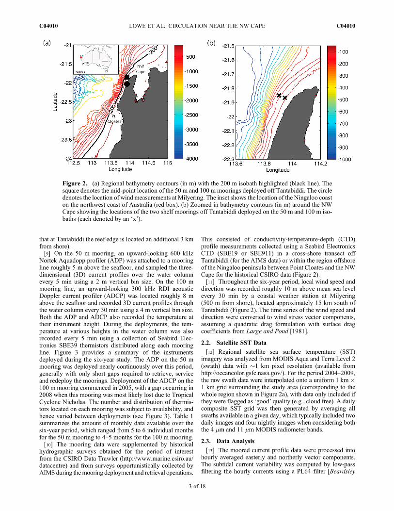
[8] The analysis focuses on field data collected off theNW Cape over a six-year period between January 2004 andDecember 2009 (Figure 2). During this period, two mooringswere maintained by the Australian Institute of MarineScience (AIMS) off Tantabiddi, deployed on the 50 m(21�52.030′ S, 113�56.817′ E) and 100 m (21�50.889′ S,113�54.288′E) isobaths (Figure 2). On this narrow section ofshelf, the 50 m and 100 m isobaths are located roughly 3 kmand 8 km, respectively, from the outer edge of the reef (note

Figure 1. A satellite sea surface temperature (in �C) imageof the NW Cape region on 16 Jan 2007 showing an extensivecold water mass adjacent to the coast.

LOWE ET AL.: CIRCULATION NEAR THE NW CAPE C04010C04010

2 of 18

that at Tantabiddi the reef edge is located an additional 3 kmfrom shore).[9] On the 50 m mooring, an upward-looking 600 kHz

Nortek Aquadopp profiler (ADP) was attached to a mooringline roughly 5 m above the seafloor, and sampled the three-dimensional (3D) current profiles over the water columnevery 5 min using a 2 m vertical bin size. On the 100 mmooring line, an upward-looking 300 kHz RDI acousticDoppler current profiler (ADCP) was located roughly 8 mabove the seafloor and recorded 3D current profiles throughthe water column every 30 min using a 4 m vertical bin size.Both the ADP and ADCP also recorded the temperature attheir instrument height. During the deployments, the tem-perature at various heights in the water column was alsorecorded every 5 min using a collection of Seabird Elec-tronics SBE39 thermistors distributed along each mooringline. Figure 3 provides a summary of the instrumentsdeployed during the six-year study. The ADP on the 50 mmooring was deployed nearly continuously over this period,generally with only short gaps required to retrieve, serviceand redeploy the moorings. Deployment of the ADCP on the100 m mooring commenced in 2005, with a gap occurring in2008 when this mooring was most likely lost due to TropicalCyclone Nicholas. The number and distribution of thermis-tors located on each mooring was subject to availability, andhence varied between deployments (see Figure 3). Table 1summarizes the amount of monthly data available over thesix-year period, which ranged from 5 to 6 individual monthsfor the 50 m mooring to 4–5 months for the 100 m mooring.[10] The mooring data were supplemented by historical

hydrographic surveys obtained for the period of interestfrom the CSIRO Data Trawler (http://www.marine.csiro.au/datacentre) and from surveys opportunistically collected byAIMS during the mooring deployment and retrieval operations.

This consisted of conductivity-temperature-depth (CTD)profile measurements collected using a Seabird ElectronicsCTD (SBE19 or SBE911) in a cross-shore transect offTantabiddi (for the AIMS data) or within the region offshoreof the Ningaloo peninsula between Point Cloates and the NWCape for the historical CSIRO data (Figure 2).[11] Throughout the six-year period, local wind speed and

direction was recorded roughly 10 m above mean sea levelevery 30 min by a coastal weather station at Milyering(500 m from shore), located approximately 15 km south ofTantabiddi (Figure 2). The time series of the wind speed anddirection were converted to wind stress vector components,assuming a quadratic drag formulation with surface dragcoefficients from Large and Pond [1981].

2.2. Satellite SST Data

[12] Regional satellite sea surface temperature (SST)imagery was analyzed from MODIS Aqua and Terra Level 2(swath) data with �1 km pixel resolution (available fromhttp://oceancolor.gsfc.nasa.gov/). For the period 2004–2009,the raw swath data were interpolated onto a uniform 1 km �1 km grid surrounding the study area (corresponding to thewhole region shown in Figure 2a), with data only included ifthey were flagged as ‘good’ quality (e.g., cloud free). A dailycomposite SST grid was then generated by averaging allswaths available in a given day, which typically included twodaily images and four nightly images when considering boththe 4 mm and 11 mm MODIS radiometer bands.

2.3. Data Analysis

[13] The moored current profile data were processed intohourly averaged easterly and northerly vector components.The subtidal current variability was computed by low-passfiltering the hourly currents using a PL64 filter [Beardsley

Figure 2. (a) Regional bathymetry contours (in m) with the 200 m isobath highlighted (black line). Thesquare denotes the mid-point location of the 50 m and 100 m moorings deployed off Tantabiddi. The circledenotes the location of wind measurements at Milyering. The inset shows the location of the Ningaloo coaston the northwest coast of Australia (red box). (b) Zoomed in bathymetry contours (in m) around the NWCape showing the locations of the two shelf moorings off Tantabiddi deployed on the 50 m and 100 m iso-baths (each denoted by an ‘x’).


3 of 18

et al., 1985] with a half-power period of 38 h (note that thisalso removed inertial motions, having a period of �32 h atthis latitude). Alongshore (x) and cross-shore (y) currentdirections were defined based on the respective major andminor axes of depth-averaged subtidal current variancecomputed from a principal component analysis of the full2004–2009 current records separately, for both the 50 m and100 m moorings [Emery and Thompson, 2001]. The major(alongshore) axis was thus oriented at �40� with respect tonorth (clockwise) for the 50 m mooring and �33� for the100 m mooring, which were then used to rotate the currentsinto their alongshore (U) and cross-shore (V) subtidal currentvelocity components (see Figure 4). To investigate the sub-tidal circulation response to local wind-forcing, the surfacewind stress vectors were also low-pass filtered with thePL64 filter to remove the diurnal sea-breeze and otherhigh frequency variability, then rotated into correspondingalongshore (ts,x) and cross-shore (ts,y) vector components.Subtidal variations in the vertical temperature structure werealso calculated at each mooring (50 m and 100 m) byapplying the PL64 filter to the raw thermistor time series.Note that for some of the temperature analysis, the data werealso high-pass filtered with a 30 day cutoff (hence band-passed) to also remove longer time scale (e.g., seasonal)changes in the annual temperature time series.[14] The alongshore and cross-shore current profiles were

used to evaluate the ‘surface’ currents (Us and Vs, respec-tively) at both the 50 m and 100 m mooring sites, by aver-aging velocities from 10 to 20 m below the surface. This

surface averaging depth was chosen since roughly the upper10 m of the water column was contaminated by sidelobeinterference for the 100 mADCP; thus a consistent averagingdepth was also applied to the shallow 50mmooring data. Thealongshore and cross-shore ‘bottom’ currents (Ub and Vb,respectively) were also computed by averaging the bottom10 m of the current profiles.[15] The dominant time scales of the variability in the

surface currents, winds and temperatures were investigatedby computing the variance preserving spectra. The responseof both the surface currents (alongshore and cross-shore) andtemperatures to wind stresses were investigated through alagged correlation analysis, with significance levels quanti-fied based on the effective degrees of freedom estimated fromthe record length divided by the autocorrelation time scale[Emery and Thompson, 2001]. The alongshore and cross-shore current profiles recorded at each mooring weredecomposed using an empirical orthogonal function (EOF)analysis to investigate the dominant modes of the verticalcurrent profile variability [Emery and Thompson, 2001].

Figure 3. Summary of mooring deployments off Tantabiddi located at the (a) 50 m isobath and (b) 100 misobath. Gray bands denote the deployment intervals for the ADP/ADCPs measuring current profilesthrough the water column; black bars denote thermistor deployment intervals and sampling depths.

Table 1. Number of Months of Data Available From the 50 m and100 m Moorings, During the Study Period 2004–2009a

Jan Feb Mar Apr May Jun Jul Aug Sep Oct Nov Dec

50 m 5 5 5 6 6 6 6 6 6 6 6 5100 m 4 4 4 5 4 4 4 4 4 4 5 4

aNote that we considered that data were available during a month when atleast two-weeks of data within a month were recorded.


4 of 18

Statistical analysis was conducted by grouping the resultsinto four ‘seasons’: (1) February–April, (2) May–July,(3) August–October, and (4) November–January. Theseperiods were chosen to capture distinct differences in thelong term averaged seasonal wind and alongshore currentconditions observed near the NW Cape (see below).[16] The historical CTD data were used to provide an

estimate of the surface mixed layer depth (MLD) variabilityduring the study period, based on a standard difference cri-teria, defined here as the minimum depth in the water columnwhen either of the following occurred [Brainerd and Gregg,1995; Condie and Dunn, 2006; Rousseaux et al., 2011]:T < T (10 m) � 0.4oC or S < S(10 m) + 0.03oC, whereT (10 m) and S(10 m) denote the temperature and salinityrecorded 10 m below the surface. Vertical temperaturestratification overwhelmingly dominated the MLD estimatesacross all seasons, with temperature controlling the MLDestimates in > 95% of the profiles. Each CTD cast was usedto compute a buoyancy frequency N ¼ ffiffiffiffiffiffiffiffiffiffiffiffiffiffiffiffiffiffiffiffiffiffiffiffiffiffiffi� g=rð Þ∂r=∂zp

. Forconsistency with, e.g., Lentz and Chapman [2004], theaverage density gradient ∂r/∂z was estimated based on thedifference between values near the surface (taken 10 m belowthe surface) and near the bottom at the 100 m isobath (taken10 m above the bottom). Each buoyancy frequency was usedto estimate the Burger number B = aN/f, where a is thebottom slope and f = 5.4 x 10�5 rad s�1 is the Coriolis fre-quency at latitude 22� S. The bottom slope a off Tantabiddiis variable, ranging from 1/80 on the inner shelf (depths< 100 m) to 1/50 on the shelf slope (depths 100–200 m). For

the Burger number calculations, an average value a = 1/65was assumed.

3. Results

3.1. Wind-Forcing

[17] Analysis of the historical wind data revealed sub-stantial seasonal variations in both the monthly averagedwind speed and direction for the region (Figure 5a). Windswere on-average relatively strong (�5 m s�1) and upwelling-favorable (i.e., in the positive alongshore direction, or towardthe northeast) during both the austral spring and summer(roughly September–February). During this period, thecross-shore component of the monthly averaged windwas roughly zero. Although periods of weaker upwelling-favorable winds did sometimes persist into early autumn(March –May), by winter (June–August) the winds were on-average much weaker (�2 m s�1) and toward the northwest(i.e., they shifted to a dominantly cross-shore direction).Variability in the low-pass filtered alongshore wind velocity(expressed in terms of its standard deviation) was relativelyconstant year-round at�2 m s�1, although somewhat greaterat the end of summer (January–March) (Figure 5b).Throughout the year, cross-shore wind variations were

Figure 4. Scatterplot of the depth-averaged currents (raweasterly and northerly components) measured at the 100 mmooring, shown for the Mar–Oct 2005 deployment as anexample. The arrows denote the rotated coordinate systemderived from the principal component analysis, with x definedas the ‘alongshore’ direction and y as the ‘cross-shore’ direc-tion. Note that the principal major axis angle differed by <3�between all deployments (comparable to the uncertainty inthe ADCP compass).

Figure 5. (a) Monthly mean alongshore and cross-shorecomponents of the wind velocity at Milyering between2004 and 2009 (refer to Figure 4 for the coordinate sys-tem). (b) Standard deviation of the low-pass filtered windvelocity components.


5 of 18

on-average smaller than alongshore variations, yet werecomparable during winter (May–July).[18] Inspection of the annual wind time series (low-pass

filtered) for a typical year cycle from 2006 (see Figure 6a)shows large fluctuations in the alongshore component of thewind velocity with periods of order 1–2 weeks. Throughoutthe year, these winds oscillated between being upwellingfavorable (i.e., positive alongshore) and relaxing to negativealongshore values. While the magnitude of these fluctuationswere larger during the late summer (i.e., January–March),they were still significant year-round (Figure 6a; see alsoFigure 5b). The variance-preserving spectrum of the along-shore component of the wind stress ts,x time series shows apeak of high energy between 7 and 14 days (Figure 7a). Thetime-scale of these strong wind fluctuations falls within a‘synoptic weather band’ that has also been identified for sitesfurther south on the Western Australian coast [Cresswellet al., 1989; Smith et al., 1991].

3.2. Seasonal Alongshore Current Variability

[19] For the 2004–2009 period, the monthly mean along-shore surface current velocities Us were relatively weak(<0.1–0.2 m s�1) at both the 50 m and 100 m mooring sites(Figure 8). Peak values of the monthly mean Us at the 50 misobath were �50% weaker than at the 100 m isobath. The

maximum southward (poleward) flow, up to 0.15 m s�1 at100 m, occurred during the austral autumn (March–May) andreached a minimum, with negligible alongshore mean flow,during spring (August–October). A similar analysis that wasconducted on the depth-averaged currents rather than surface(not shown), gave similar results to Figure 8, both in termsof the magnitude and phasing.[20] For the example shown for 2006 in Figure 6b,

the magnitude of the alongshore surface current fluctuationsUs are much greater than the monthly mean values, withvalues oscillating between �0.8 m s�1 during some events.Inspection of the variance preserving spectra ofUs at both the50 m and 100 m isobaths (Figure 7b), both show a well-defined peak with a period of roughly two weeks. This cur-rent peak of �2 weeks is thus narrower, but includes thewider�1–2 week peak associated with the wind-forcing. Wenote that the peak in current energy at �2 weeks has norelationship to the spring-neap cycle of the tide, i.e., thecorrelation between the low-pass filtered alongshore currentsand the envelope of the local tide gauge data computed via aHilbert transform [Emery and Thompson, 2001] was notsignificant (correlation < 0.05, not shown). Instead, it appearsthat some of the energy in the wind fluctuations was shiftedto drive current motions with slightly lower frequencies (thisissue is discussed in further detail in section 4.1). Analysis of

Figure 6. Time series of the low-pass filtered (a) alongshore component of the wind velocity, (b) along-shore surface current Us at the 50 m and 100 m isobaths, and (c) near-bottom temperature measured on the50 m isobath, for the period of 2006.


6 of 18

the full historical record (2004–2009), shows that the mag-nitude of these alongshore current fluctuations (characterizedby the standard deviation in Figure 8b) were always greaterthan the monthly mean values (by a factor > 2), implying thatthe currents off the NWCape reversed episodically during allmonths of the year. While the magnitude of the variabilitywas comparable year-round, a peak occurred in June at the50 m isobath (Figure 8b). At the 100 m isobath, a minor peak

also occurred in June; however, the greatest variabilityoccurred during January–February.[21] The alongshore surface current variability Us at the

50 m isobath was reasonably well-correlated with thealongshore wind stress ts,x, with maximum correlationcoefficients ranging from Rwind �0.4–0.6 when the currentslagged the wind by Lagwind �7–10 h (Table 2). These max-imum correlations were somewhat higher during winter andspring periods (May–October) with Rwind �0.6, and werelowest during the late-summer (February–April) period withRwind �0.4. The response of the bottom currents Ub wasnearly identical to the surface currents (Table 2), consistentwith the water column < 50 m being well-mixed (see below).

Figure 7. Variance preserving spectra of (a) the alongshore component of the wind stress ts,x and (b) thealongshore surface current Us at the 50 m and 100 m mooring sites, for 2006 (i.e., for the same time seriesin Figures 6a and 6b).

Figure 8. Monthly (a) mean and (b) standard deviation inthe alongshore surface current recorded at the 50 m and100 m isobaths, during the period 2004–2009.

Table 2. Lagged Cross-Correlation Analysis Between the Along-shore Wind Stress tx and Alongshore Surface Us and Bottom Ub

Currents Measured by the 50 m and 100 m Moorings, Reportedfor Four Seasonal Periodsa

Feb–Apr May–Jul Aug–Oct Nov–Jan

50 mRwind (surface) 0.44 � 0.03 0.58 � 0.03 0.56 � 0.02 0.51 � 0.10Lagwind (surface) +10 � 4 h +9 � 3 h +8 � 3 h +8 � 2 hRwind (bottom) 0.42 � 0.03 0.57 � 0.03 0.56 � 0.02 0.48 � 0.10Lagwind (bottom) +9 � 4 h +9 � 3 h +8 � 3 h +7 � 2 h

100 mRwind (surface) 0.45 � 0.03 0.52 � 0.05 0.50 � 0.02 0.53 � 0.08Lagwind (surface) +12 � 5 h +14 � 4 h +16 � 2 h +11 � 3 hRwind (bottom) 0.25 � 0.05 0.51 � 0.05 0.43 � 0.04 0.43 � 0.09Lagwind (bottom) +8 � 5 h +16 � 3 h +17 � 2 h +8 � 2 h

aRwind denotes the maximum correlation value at a lag interval Lagwind inhours (note that a positive value implies the current lags the wind). Allcorrelation values were significant to the 99% confidence level. Values areexpressed as mean �1 standard deviation, based on the variability in themean seasonal values computed between each individual year.


7 of 18

[22] Further offshore at the 100 m isobath, values of Rwind

between the alongshore surface currents and wind stresswere comparable (�0.5) to the 50 m site; however, the sur-face currents lagged the winds by several additional hours(Lagwind �11–16 h) (Table 2). Values of Rwind and Lagwindbetween the bottom currents Ub and surface wind stresses atthe 100 m isobath, were comparable to the surface valuesduring the periods from May–January. However, during theFebruary–April period, the alongshore bottom currents werepoorly correlated with the winds (Rwind � 0.25).

3.3. Mixed-Layer Depth and Current ProfileVariability

[23] Vertical temperature profiles from the historical CTDcasts were grouped according to season (Figure 9). Duringthe late-summer period (Feb–Apr) there was a relativelyshallow and consistent MLD of�50 m (standard deviation ofonly�10 m) (see Table 3). The MLD significantly deepened

during the May–October period (mean values of 120–130 m), yet this value was highly variable (standard deviationof 40–60 m). During the November–January period (earlysummer) the water column began re-stratifying, but the MLDwas still relatively deep during this period, averaging�90 m.[24] The alongshore and cross-shore current profiles were

time-averaged within each seasonal period (Figure 10). Theanalysis reported here focuses on profile data from the 100 mmooring, with any differences with the 50 m mooring datareported in the text below. The mean (3-month averaged)alongshore current profilesU(z) were variable between years,particularly in the May–July and November–January periods(Figures 10a–10d). However, in most seasons the alongshorecurrents were on-average strongly sheared, with strongestpoleward (negative) currents occurring near the middle orwithin the bottom half of the water column. The alongshoreflow near the surface was slightly weaker, likely in responseto the opposing northward (equatorward) wind stress that

Figure 9. Temperature profiles from the historical CTD casts grouped by season: (a) Feb–Apr, (b) May–Jul, (c) Aug–Oct, and (d) Nov–Jan. The gray dotted lines denote individual CTD casts and the thick blackline represents the mean profile. The horizontal solid line represents the mean MLD for the period and thehorizontal dotted lines denote the range, based on the standard deviation (see Table 3).

Table 3. Seasonal Stratification Statisticsa


MLD (m) 51 � 14 136 � 40 123 � 55 94 � 27N (rad s�1) 1.19 � 0.21 � 10�2 0.38 � 0.19 � 10�2 0.37 � 0.21 � 10�2 0.53 � 0.14 � 10�2

B 3.31 � 0.48 1.02 � 0.54 0.97 � 0.43 1.47 � 0.24∂T/∂x (�C m�1) 5.2 � 0.09 � 10�6 2.3 � 0.08 � 10�6 5.5 � 0.05 � 10�6 6.2 � 0.07 � 10�6

aMLD denotes the computed mixed layer depth (mean� standard deviation) derived from the historical temperature profiles shown in Figure 9. N denotesthe buoyancy frequency and B is the corresponding Burger number (see section 2.3 for details). ∂T/∂x represents the seasonal mean alongshore temperaturegradient off the Ningaloo coast inferred from the historical MODIS SST imagery. Values are expressed as mean �1 standard deviation, based on the var-iability in the mean seasonal values computed for each individual year.


8 of 18

was present most of the year (Figure 5a). The correspondingseasonal mean cross-shore current profiles V(z) were gener-ally much weaker (typically <0.02 m s�1), yet were variable(Figures 10e–10h). During many of the periods there wassome consistency in the seasonal-averaged profiles betweenyears, with some evidence of downwelling on-averageduring winter periods (May–July in particular), where near-bottom velocities tended to be weakly directed offshore(positive), and some evidence of weak upwelling on-averagein summer (February–April) with a weak offshore-directedflow near the surface.[25] Results from the EOF analysis were used to investi-

gate seasonal differences in the response of the alongshore

and cross-shore subtidal current profile variability, againfocusing on the 100 m mooring data. The first alongshoreEOF mode (Figures 11a–11d) explained the vast majorityof the total variance observed year-round (�95%; Table 4),and displayed a unidirectional profile structure with a gradualdecrease in current speed below the water surface. Althoughthere were not large differences in the alongshore EOFmode 1 profile shapes between seasons, during summerperiods (February–April and November–January), stronger

Figure 10. Seasonal mean (a–d) alongshore and (e–h)cross-shore current profiles for the four seasons, recorded atthe 100 m mooring. The series of solid lines in each figurerepresent individual mean current profiles (i.e., each repre-senting the seasonal average profile for an individual year).The circles denote the mean profile averaged across all years.Note the difference in the scale between the alongshore andcross-shore velocities.

Figure 11. EOF mode shapes for the alongshore currentprofiles at 100 m, grouped by season: (a–d) mode 1 profilesand (e–h) mode 2 profiles. Data are shown for the periods:Feb–Apr (Figures 11a and 11e), May–Jul (Figures 11b and11f), Aug–Oct (Figures 11c and 11g), and Nov–Jan(Figures 11d and 11h). Note that the first mode was arbitrarilynormalized by the maximum value, while the second modewas normalized by the maximum onshore (negative) value.The series of solid lines in each figure represent the seasonalprofile obtained during different years. The circles denotethe seasonal profile averaged over the entire 6 year study.


9 of 18

shear occurred in the top of the water column at a pointroughly 40 m below the surface (Figures 11a and 11d), thuscomparable to the shallowest MLD during summer(Figure 9). The time-varying amplitude of the first along-shore EOFmode (not shown) was moderately correlated withthe alongshore wind stress ts,x (Rwind � 0.5), when the modelagged the wind by roughly half a day (Table 4); as expected,these values are nearly identical to those based on thealongshore surface currents alone in Table 2. The secondalongshore EOF mode (Figures 11e–11h) displayed a first-mode baroclinic structure with the single zero-crossing nearthe middle of the water column (�50 m depth) throughoutthe year. This second alongshore mode explained a verysmall percentage of the variance (typically 3%); however,during the February–April period this mode explainedslightly more variance (�5%) and was also better correlatedwith the alongshore wind stresses (Rwind � 0.3) (Table 4).[26] The percentage of the variance in the cross-shore

subtidal current profiles was more evenly distributedbetween the first two EOF modes (Table 4). The first cross-shore EOF mode explained only 50–60% of the variance.While these profiles were unidirectional, a small subsurfacemaximum was present at roughly 30–40 m depth during thesummer periods (February–April and November–January)(Figures 12a–12d). This first mode, however, was not cor-related with the alongshore wind stress (Rwind only �0.1).The second cross-shore EOF mode typically explained�25% of the variance (Table 4), and displayed two some-what different profile shapes during the year (Figures 12e–12h). During the winter periods (May–July and August–October), a first-mode baroclinic shape was identified, withnear-surface and near-bottom extrema and a zero-crossing

near the middle of the water column (Figures 12f and 12g).During the summer periods (February–April and November–January), a negative subsurface maximum occurred near themiddle of the water column, with a zero crossing typically30 m below the surface (Figures 12e and 12h). Both sets ofprofiles display characteristics of an upwelling shape: posi-tive (offshore-directed) flow near the surface and negative(onshore-directed) flow near the bottom, when the sign of the

Figure 12. EOF mode shapes for the cross-shore currentprofiles at 100 m, grouped by season: (a–d) mode 1 profilesand (e–h) mode 2 profiles. Data are shown for the periods:Feb–Apr (Figures 12a and 12e), May–Jul (Figures 12b and12f), Aug–Oct (Figures 12c and 12g), and Nov–Jan(Figures 12d and 12h). Note that the first mode was arbi-trarily normalized by the maximum value, while the secondmode was normalized by the maximum onshore (negative)value. The series of solid lines in each figure represent theseasonal profile obtained during different years. The circlesdenote the seasonal profile averaged over the entire 6 yearstudy.

Table 4. Response of the EOF Current Profile Modes at 100 m(Alongshore and Cross-Shore) to the Alongshore Wind Stress,Grouped by Seasona


Alongshore EOFmode 1Percent variance 93 � 1 95 � 1 95 � 1 95 � 1Rwind 0.47 � 0.10 0.51 � 0.11 0.50 � 0.10 0.49 � 0.13Lagwind 6 � 5 12 � 7 14 � 7 13 � 7

Alongshore EOFmode 2Percent variance 5 � 1 3 � 1 3 � 1 3 � 1Rwind 0.32 � 0.07 0.22 � 0.11b 0.20 � 0.12b 0.25 � 0.13Lagwind 28 � 10 41 � 17 39 � 16 35 � 14

Cross-shore EOFmode 1Percent variance 50 � 5 60 � 11 62 � 10 61 � 11Rwind (0.09 � 0.06) (0.10 � 0.06) (0.11 � 0.07) 0.14 � 0.07b

Lagwind 86 � 18 72 � 33 64 � 32 58 � 35Cross-shore EOFmode 2Percent variance 26 � 2 24 � 5 24 � 5 24 � 6Rwind 0.30 � 0.02 0.41 � 0.15 0.41 � 0.13 0.37 � 0.14Lagwind 2 � 1 4 � 2 4 � 2 6 � 2

a‘Percent variance’ denotes the percentage of the total variance of thecurrent profiles explained by that mode. Rwind and Lagwind denote themaximum correlation and associated lag interval, between the time-varying EOF modal amplitude and the alongshore wind stress. Correlationvalues italicized in parentheses were not significant to the 95% confidencelevel. Values are expressed as mean �1 standard deviation, based on thevariability in the mean seasonal values computed for each individual year.

bValues were not significant to the 99% confidence level.


10 of 18

time-varying amplitude of this mode was positive. Thus thesecond cross-shore EOF mode was positively correlated withan equatorward (positive) alongshore wind stress ts,x year-round (Rwind typically �0.4), although the correlation wasslightly lower during the February–April period (Rwind = 0.3).This may be due to the mean poleward flow being strongestduring the February–April period (Figure 8), which couldimply that the pressure gradient opposing the southerly windstresses was strongest during this time of year, and thushaving more influence on the cross-shore upwelling/down-welling response. In general, the response time for the cross-shore second EOF mode was only a few hours, and hencemuch faster than the alongshore EOF mode 1 response ofroughly half a day. These lag times between the wind-forcingand each current component is consistent with both theory[e.g., Brink, 1983] and observations from other inner shelfregions [e.g., Cudaback and Largier, 2001], which indicatethe alongshore flow should respond within one half of aninertial period (roughly half a day at this site), whereas thecross-shore transport should respond almost instantaneously.

3.4. Seasonal Temperature Variability

[27] The monthly averaged SSTs recorded by the upperthermistor on the 50 m mooring (�10 m below the surface)revealed a seasonal cycle with a maximum temperature of�28�C in autumn (April) and a minimum of�23�C in spring(October) (Figure 13a). The phasing of this seasonal SSTvariability is very similar to the cycle observed off the much

better studied southwest coast of Australia (near �32�S)[Feng et al., 2003]. Temperature fluctuations, expressed interms of the standard deviation observed within each month,were greatest (�1.5�C) during summer (January–March),with a secondary peak (up to �1.0�C) during most yearsaround June (Figure 13b).[28] SST data obtained from historical MODIS satellite

imagery (SSTMODIS), extracted for the nearest 1 km pixelsurrounding the 50 m mooring site, were compared againstthe near-surface temperatures recorded in situ from themooring (SSTmooring) during the same day. Results from alinear least squares regression between the data (derived fromn = 1935 samples) revealed excellent agreement, with theregression relationship SSTMODIS = 1.02 SSTmooring + 0.4�C(R2 = 0.93). The MODIS SST was thus on-average slightlywarmer than the mooring data, which may partially be due tothe mooring measurements occurring 10 m below the surfacerather than directly at the surface. As the monthly mean andstandard deviations of the MODIS SST data (Figures 13b and13d) agreed very well with the corresponding mooring values(Figures 13a and 13c), the data can thus reliably provide abroader context on the spatial variability in SST across theNingaloo coastal region.[29] Monthly averaged regional maps of SST for the region

show large differences in the spatial variability over a sea-sonal cycle (Figure 14). During the summer months of March(Figure 14a) and December (Figure 14d), a narrow band ofcool water (�10 km wide) near the coast extended up the

Figure 13. Sea surface temperature statistics at (a and c) the 50 m isobath recorded on the mooring and(b and d) from the nearest 1 km MODIS satellite SST imagery pixel. The monthly mean (Figure 13a)and standard deviation (Figure 13c) of the SST recorded by the upper-most thermistor on the 50 mmooring(�10 m below the surface). The corresponding mean (Figure 13b) and standard deviation (Figure 13d) ofthe SST observed from the MODIS images.


11 of 18

entire Ningaloo peninsula. Conversely, in June an �40 kmwide region of warm water extended down the coast from theNW Cape (Figure 14b). During September, the temperaturefield off the Ningaloo peninsula was mostly characterized by

an alongshore temperature gradient, with minimal cross-shore variation (Figure 14c). Analysis of the historicalmonthly SST temperature variability (expressed in terms ofthe standard deviation), revealed that the variability is at a

Figure 14. Long-term (2004–2009) monthly averaged SST images shown for: (a) March, (b) June,(c) September, and (d) December. Note that to highlight spatial temperature differences the color bar axiswas chosen as �1� from the monthly mean SST off Tantabiddi (see Figure 13).


12 of 18

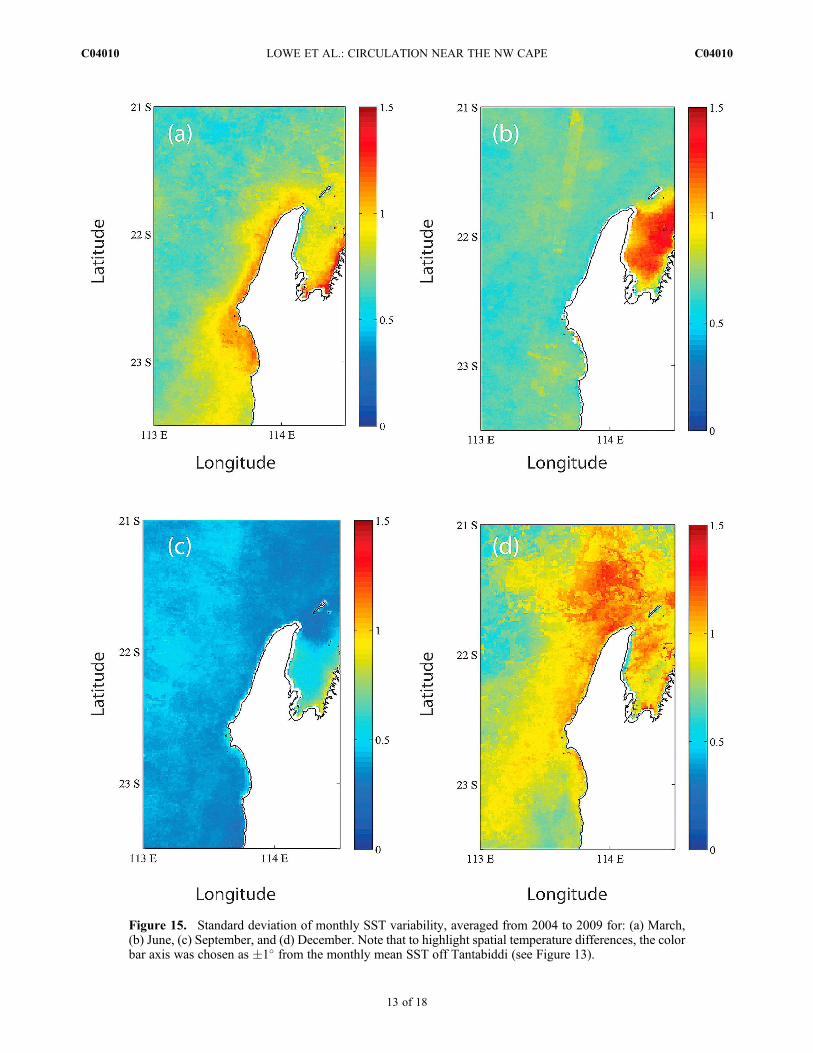
Figure 15. Standard deviation of monthly SST variability, averaged from 2004 to 2009 for: (a) March,(b) June, (c) September, and (d) December. Note that to highlight spatial temperature differences, the colorbar axis was chosen as �1� from the monthly mean SST off Tantabiddi (see Figure 13).


13 of 18

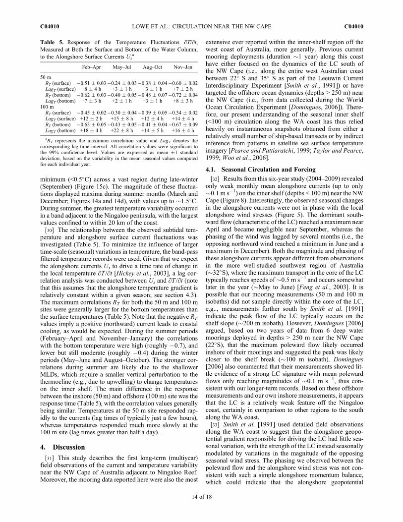
minimum (<0.5�C) across a vast region during late-winter(September) (Figure 15c). The magnitude of these fluctua-tions displayed maxima during summer months (March andDecember; Figures 14a and 14d), with values up to �1.5�C.During summer, the greatest temperature variability occurredin a band adjacent to the Ningaloo peninsula, with the largestvalues confined to within 20 km of the coast.[30] The relationship between the observed subtidal tem-

perature and alongshore surface current fluctuations wasinvestigated (Table 5). To minimize the influence of largertime-scale (seasonal) variations in temperature, the band-passfiltered temperature records were used. Given that we expectthe alongshore currents Us to drive a time rate of change inthe local temperature ∂T /∂t [Hickey et al., 2003], a lag cor-relation analysis was conducted between Us and ∂T /∂t (notethat this assumes that the alongshore temperature gradient isrelatively constant within a given season; see section 4.3).The maximum correlations RT for both the 50 m and 100 msites were generally larger for the bottom temperatures thanthe surface temperatures (Table 5). Note that the negative RT

values imply a positive (northward) current leads to coastalcooling, as would be expected. During the summer periods(February–April and November–January) the correlationswith the bottom temperature were high (roughly �0.7), andlower but still moderate (roughly �0.4) during the winterperiods (May–June and August–October). The stronger cor-relations during summer are likely due to the shallowerMLDs, which require a smaller vertical perturbation to thethermocline (e.g., due to upwelling) to change temperatureson the inner shelf. The main difference in the responsebetween the inshore (50 m) and offshore (100 m) site was theresponse time (Table 5), with the correlation values generallybeing similar. Temperatures at the 50 m site responded rap-idly to the currents (lag times of typically just a few hours),whereas temperatures responded much more slowly at the100 m site (lag times greater than half a day).

4. Discussion

[31] This study describes the first long-term (multiyear)field observations of the current and temperature variabilitynear the NW Cape of Australia adjacent to Ningaloo Reef.Moreover, the mooring data reported here were also the most

extensive ever reported within the inner-shelf region off thewest coast of Australia, more generally. Previous currentmooring deployments (duration �1 year) along this coasthave either focused on the dynamics of the LC south ofthe NW Cape (i.e., along the entire west Australian coastbetween 22� S and 35� S as part of the Leeuwin CurrentInterdisciplinary Experiment [Smith et al., 1991]) or havetargeted the offshore ocean dynamics (depths > 250 m) nearthe NW Cape (i.e., from data collected during the WorldOcean Circulation Experiment [Domingues, 2006]). There-fore, our present understanding of the seasonal inner shelf(<100 m) circulation along the WA coast has thus reliedheavily on instantaneous snapshots obtained from either arelatively small number of ship-based transects or by indirectinference from patterns in satellite sea surface temperatureimagery [Pearce and Pattiaratchi, 1999; Taylor and Pearce,1999; Woo et al., 2006].

4.1. Seasonal Circulation and Forcing

[32] Results from this six-year study (2004–2009) revealedonly weak monthly mean alongshore currents (up to only�0.1 m s�1) on the inner shelf (depths < 100 m) near the NWCape (Figure 8). Interestingly, the observed seasonal changesin the alongshore currents were not in phase with the localalongshore wind stresses (Figure 5). The dominant south-ward flow (characteristic of the LC) reached a maximum nearApril and became negligible near September, whereas thephasing of the wind was lagged by several months (i.e., theopposing northward wind reached a minimum in June and amaximum in December). Both the magnitude and phasing ofthese alongshore currents appear different from observationsin the more well-studied southwest region of Australia(�32�S), where the maximum transport in the core of the LCtypically reaches speeds of�0.5 m s�1 and occurs somewhatlater in the year (�May to June) [Feng et al., 2003]. It ispossible that our mooring measurements (50 m and 100 misobaths) did not sample directly within the core of the LC,e.g.., measurements further south by Smith et al. [1991]indicate the peak flow of the LC typically occurs on theshelf slope (�200 m isobath). However, Domingues [2006]argued, based on two years of data from 6 deep watermoorings deployed in depths > 250 m near the NW Cape(22�S), that the maximum poleward flow likely occurredinshore of their moorings and suggested the peak was likelycloser to the shelf break (�100 m isobath). Domingues[2006] also commented that their measurements showed lit-tle evidence of a strong LC signature with mean polewardflows only reaching magnitudes of �0.1 m s�1, thus con-sistent with our longer-term records. Based on these offshoremeasurements and our own inshore measurements, it appearsthat the LC is a relatively weak feature off the Ningaloocoast, certainly in comparison to other regions to the southalong the WA coast.[33] Smith et al. [1991] used detailed field observations

along the WA coast to suggest that the alongshore geopo-tential gradient responsible for driving the LC had little sea-sonal variation, with the strength of the LC instead seasonallymodulated by variations in the magnitude of the opposingseasonal wind stress. The phasing we observed between thepoleward flow and the alongshore wind stress was not con-sistent with such a simple alongshore momentum balance,which could indicate that the alongshore geopotential

Table 5. Response of the Temperature Fluctuations ∂T/∂t,Measured at Both the Surface and Bottom of the Water Column,to the Alongshore Surface Currents Us

a


50 mRT (surface) �0.51 � 0.03�0.24 � 0.03�0.38 � 0.04�0.60 � 0.02LagT (surface) +8 � 4 h +3 � 1 h +3 � 1 h +7 � 2 hRT (bottom) �0.62 � 0.03�0.40 � 0.05�0.48 � 0.07�0.72 � 0.04LagT (bottom) +7 � 3 h +2 � 1 h +3 � 1 h +8 � 3 h

100 mRT (surface) �0.45 � 0.02�0.30 � 0.04�0.39 � 0.05�0.34 � 0.02LagT (surface) +12 � 2 h +15 � 8 h +12 � 4 h +14 � 4 hRT (bottom) �0.63 � 0.05�0.43 � 0.05�0.41 � 0.04�0.67 � 0.09LagT (bottom) +18 � 4 h +22 � 8 h +14 � 5 h +16 � 4 h

aRT represents the maximum correlation value and LagT denotes thecorresponding lag time interval. All correlation values were significant tothe 99% confidence level. Values are expressed as mean �1 standarddeviation, based on the variability in the mean seasonal values computedfor each individual year.


14 of 18

gradient is not constant throughout the year, as proposed byGodfrey and Ridgway [1985]. However, seasonal variationsin the source waters of the LC could also explain theobserved phasing between the alongshore wind stress and thepoleward flow. It is well known that the LC accelerates downthe west coast of Australia, with at least some of its watersourced from onshore geostrophic flow between 22� and30�S [Smith et al., 1991;Domingues et al., 2007]. Smith et al.[1991] speculated that there may also be some seasonal var-iation in these source waters, with more onshore entrainmentof subtropic waters south of 22�S during late winter (�July toSeptember) and conversely a more tropical water source fromthe North West Shelf during autumn (�March to May). Ourmeasurements are consistent with this theory, with the pole-ward shelf current off Ningaloo (21�S) peaking in autumn(�April), and hence somewhat earlier than further south.This picture is also consistent with seasonal current obser-vations on the southern North West Shelf (�300 km to thenorthwest) [Holloway and Nye, 1985]. There, a consistent(year-round) poleward flow has not been observed; however,a relatively strong (�0.2 m s�1) seasonal poleward flow doesoccur, peaking near April. This phasing agrees with ourobservations, suggesting that the coastal waters off Ningaloo(and the well-defined LC south of 22�S) are seasonallysourced from northern tropical waters and thus strong con-nectivity occurs with the North West Shelf primarily duringautumn, with likely only weak connectivity during othertimes of the year.[34] Despite the weak seasonal mean currents observed off

the Ningaloo coast, the alongshore flows were characterizedby large subtidal velocity fluctuations with periods of�1–2 weeks (Figures 6b and 7b). On-average over the year,the magnitude of these alongshore current fluctuations(Figure 8b) were typically at least twice as large as thebackground mean currents (Figure 8a), implying the systemexperiences frequent alongshore current reversals. Thesecurrent fluctuations were moderately correlated with the localwind-forcing (Table 2). The dominant time-scale of thewind-forcing falls within the synoptic band of weather pat-terns (�1–2 weeks) in the Western Australia region [Gentilli,1972], which has also been observed to dominate the currentvariability at other locations further south on this coast, i.e.,near 30� S [Cresswell et al., 1989]. Nevertheless, Figure 7does show a slight shift in the spectral peaks of the localwind-forcing (peak �9 days) and the alongshore currents(peak �14 days). Some of this shift to lower frequencieswould be due to the time-scale associated with the accelera-tion of the alongshore flow by local wind-forcing; however,the observations indicate that this local response occurs overa period of order one day (see Table 2), which is also con-sistent with the response time observed on other inner shelves[see Lentz and Fewings, 2012]. This indicates that thealongshore current variability cannot be solely explained by asimple alongshore momentum balance forced by the localwinds, i.e., the results show that a significant portion of thealongshore current variability is still not explained by thelocal wind-forcing (see Table 2).[35] These results have some similarity to observations on,

for example, the Northern California shelf by Largier et al.[1993], who observed a much more dramatic separation inthe spectral peaks between the wind-forcing and the along-shore currents (i.e., roughly 4–7 days versus 15–30 days,

respectively). They described variability in the currents asoccurring within a “very low-frequency” band, suggestingthat this arose from a decoupling of the forcing in the higherfrequency “wind band” through larger-scale interactionsoccurring within the deeper ocean. Given the localizedmooring observations of the shelf circulation in this presentstudy, the role of mesoscale ocean processes on Ningaloo’sshelf circulation (including its relationship to regional-scalewind-forcing) remains unclear. But it is clear that other(unexplained) sources of alongshore current variability mayhave a strong influence on this coast. For example, this maybe due to coastally trapped waves remotely generated byatmospheric forcing [Eliot and Pattiaratchi, 2010], as well asthe encroachment of mesoscale eddies onto the shelf [Fenget al., 2005], which may ultimately be generated by wind-forcing (albeit indirectly and on different time scales).[36] Results from these long-term current records from the

Ningaloo shelf also reveal that water rarely flows eithercontinuously poleward or equatorward for extended periodsof time (i.e., for durations greater than a few weeks) duringall months of the year. This contradicts suggestions in theliterature that the mean shelf circulation off Ningaloo Reefdisplays a strong seasonal cycle. While recognized as atransient system, the Ningaloo coast is conventionallyassumed to be primarily dominated by a poleward (south-ward) flowing LC during winter months and an equatorward(northward) flowing NC during summer months [e.g., Taylorand Pearce, 1999]. Unexpectedly, our results showed noevidence of a consistent equatorward flow at any time of year(Figure 8a), and certainly no consistent signature of anequatorward NC during summer months (September–April)when it has been proposed to be at its strongest [Taylor andPearce, 1999; Woo et al., 2006]. While there are relativelyshort periods of equatorward flow, the lack of a monthlymean equatorward (northward) flow during any time of yearon the inner-shelf raises doubts about whether the NC shouldreally be viewed as a true current system in the formal sense.[37] In general, the highly transient nature of the shelf

circulation off the Ningaloo coast is not entirely unique whencompared with other western boundary coastal regionsglobally. For example, alongshore currents on the inner shelfof California and Oregon do periodically reverse duringperiods when the predominantly upwelling-favorable windsrelax [e.g., Bane et al., 2005; Melton et al., 2009]. However,the main difference between the Ningaloo coast and otherwestern boundary coastal upwelling systems globally, wouldbe the presence of a comparatively large poleward pressuregradient that persists year-round along the entire west coastof Australia. As a result, the shelf circulation off the Ningaloocoast appears to be in a continuous transient state (seeFigure 6b), with a lack of sustained (time scales of weeks tomonths) equatorward flow that is a prominent feature ofclassic upwelling coasts.

4.2. Temperature and Current Profile Variability

[38] Long-term hydrographic measurements in the regionshowed that the MLD varied seasonally from as shallowas �50 m in late summer (February–April) to as deep as�130 m in winter (May–June) (Figure 9). These very deepMLDs observed in winter off the Ningaloo coast are consis-tent with observations by Rousseaux et al. [2011], whoexamined the role of the MLD deepening in the context of the


15 of 18

seasonal winter phytoplankton bloom observed in the region.Rousseaux et al. [2011] proposed that the deepening of theMLD was driven by a combination of winter convectivemixing and the strengthening LC in autumn. Lourey et al.[2006] developed a MLD climatology for the southwestregion of WA (south of 26� S) and indicated values of up to80 m for coastal regions within the LC during winter.Rousseaux et al. [2011] investigated the spatial variation inMLDs for the broader northwest region and found the dee-pest values (up to�140 m) were confined to a narrow coastalregion (<40 km wide) off the Ningaloo coast, suggesting thismay be a relatively localized phenomenon.[39] The structure of the subtidal current profiles differed

significantly in response to changes in the seasonal stratifi-cation, as revealed by the EOF analysis. For the alongshorecurrent profiles, the first EOF mode explained �95% of thevariance year-round, characterized by a unidirectional flowthat monotonically increased above the bottom (Figure 11).During winter periods (May–Jul, Aug–Oct) when MLDswere >100 m (comparable or greater than the deepestmooring site), the greatest shear in the alongshore currentprofiles occurred adjacent to the seafloor (<30 m above thebottom) within the unstratified water column (Figures 11band 11c). However, during summer periods (Feb–Apr,Nov–Jan) the region of maximum shear shifted upwards towithin 30–40 m of the surface, as a result of the significantshallowing of the MLD during summer (Figures 11aand 11d). This first alongshore EOF mode was reasonablywell-correlated with the alongshore wind stress year-round(Rwind�0.5).[40] A majority (but still only 50–60%) of the variability in

the cross-shore current profiles was also explained by a first(unidirectional flow) EOF mode; however, this cross-shoremode was poorly correlated with the local wind stresses(Rwind ≲ 0.1). This mode likely reflects the migration of wateron and off the shelf, e.g., due to the meandering of the LC, theencroachment of mesoscale eddies, etc., in the region.[41] The second cross-shore EOF mode, however, also

explained a significant amount of the cross-shore currentvariability (up to �30%), and this mode was fairly well-correlated (Rwind � 0.4) with the alongshore wind stress(Figures 12e–12h). The profile shapes of this second EOFmode were consistent with an upwelling profile (or down-welling depending on the sign of the EOF modal amplitude),i.e., a positive (equatorward) alongshore wind stress drovean offshore near-surface flow that was replenished by anonshore flow below. However, two seasonal differences inthe profile shapes were observed: a maximum onshore flowoccurred near the bottom during winter months (Figures 12fand 12g), whereas a maximum onshore flow occurred nearthe middle of the water column during summer periods(Figures 12e and 12h). This shift in the vertical position of theonshore return flow is consistent with seasonal changes in theBurger number B resulting from changes in the local seasonalstratification (Table 3). Through comparison of the dominantcross-shore current profiles from a number of upwellingregions globally, as well as using results from idealizednumerical modeling, Lentz and Chapman [2004] proposedthat for upwelling under conditions of weak stratification(B < 1), the onshore return flow occurs within the bottomboundary layer, whereas for conditions of relatively strongstratification (B�1 or larger), the location of the return flow

shifts to the interior of the water column. The seasonalupward shift in the position of the onshore return flow offNingaloo (Figures 12e–12h) appears consistent with theseexpected trends, with the local Burger number increasingfrom �1 during winter to �3 in summer. The differences inthe profile shapes do occur for larger values of B (>1) than thetheory suggests, which could possibly be due to the variableslope off Tantabiddi, i.e., if the slope of the inner shelf regiona = 1/80 is used instead of the average slope, values of B arefurther reduced. Nevertheless, this suggests that wind-drivencoastal upwelling can occur year-round along this coast;however, the onshore-flowing water supporting this upwell-ing likely comes from a deeper source in winter comparedto summer.

4.3. Sources of Temperature Fluctuations:Upwelling Versus Advection?

[42] The temperature fluctuations (∂T /∂t) observed alongthe Ningaloo coast were well-correlated with variability inthe alongshore currentsUmeasured the inner-shelf; however,this observation does not distinguish between the variousmechanisms that may contribute to these temperature chan-ges. For example, although the historical current profilerecords reveal that transient coastal upwelling occurs alongthis coast, which would contribute to a cooling of the innershelf, it is also possible that the associated northward flowthat advects cooler surface waters from the south, couldcontribute (or even make the dominant contribution) to theobserved coastal cooling events. To investigate the potentialimportance of these mechanisms to the inner-shelf heatbudget, we investigated the magnitude of the terms respon-sible for the temperature fluctuations (∂T /∂t) using a simpleheat budget equation [e.g., Hickey et al., 2003]

∂T∂t

¼ �U∂T∂x

�W∂T∂z

; ð1Þ

where the second term of equation (1) describes temper-ature changes driven by alongshore advection, while the thirdterm describes contributions from vertical transport mech-anisms (i.e., due to upwelling/downwelling). We note thatequation (1) neglects other processes such as radiative heat-ing, wind mixing, as well as cross-shore advection.[43] To investigate the importance of the terms in

equation (1) using the long-term mooring records, we useddirect measurements of the low-pass filtered temperaturefluctuations (∂T /∂t) to evaluate the first term. For the secondterm, we used measurements of the alongshore surface cur-rents Us and estimated the alongshore temperature gradient(∂T /∂x) from the seasonally averaged MODIS surface tem-perature fields. We could not accurately compute the thirdterm from the mooring data, due to the weak vertical veloc-ities and the sparsely resolved temperature profile data fromthe thermistors. Therefore, for this analysis we investigatedhow much of the variability in the observed temperaturefluctuations could be explained by the alongshore advectionterm alone. Figure 16 indicates that only a very small amount(�10–20%) of the observed temperature variability can beexplained by alongshore advection, indicating that by defaultthe vertical advection (upwelling/downwelling) term waslikely significant. Ultimately, the detailed dynamics ofupwelling and its role in the coastal heat budget will be most


16 of 18

accurately quantified with 3D numerical modeling (a numer-ical model of the Ningaloo coast using the Regional OceanModeling System is presently being developed by J. Xu et al.(Dynamics of the summer shelf circulation and transientupwelling off Ningaloo Reef, Western Australia, submittedto Journal of Geophysical Research, 2012)). Nevertheless,the results from this field study suggest that coastal upwellingis episodically very important along this coast; however, thisis importantly not restricted to summer months. Both thecurrent profile analysis (Table 4) and heat balance analysis(Table 5) suggest that upwelling occurs with roughly thesame frequency during all seasons, driven by the variabilityin wind-forcing in the synoptic weather band (1–2 weeks)that persists throughout the year.

5. Conclusions

[44] Results from the first long-term study of the circula-tion and temperature variability on the Ningaloo coast nearthe NW Cape have revealed a transient inner shelf systemwith little consistency in flow during any time of the year.The shelf circulation was controlled by a balance between thelarge-scale poleward pressure gradient present along theentire WA coast countered by periodic opposing southerly(equatorward) wind events that occurred year-round withperiods of roughly 1–2 weeks. These local wind stressescyclically overcame the poleward pressure gradient, causingthe inner shelf circulation to alternate between being pole-ward and equatorward throughout the year. The magnitude ofthese 1–2 week alongshore current fluctuations were muchlarger than the weak seasonal mean currents along this coast.In particular, these observations do not support the presenceof a consistent equatorward (northward) flowing currentalong the Ningaloo coast during summer months (Septemberto April), referred to in the literature as the Ningaloo Current.[45] The transient nature of the shelf circulation on the

Ningaloo coast also implies that patterns of connectivity,

both within Ningaloo Reef itself and, on regional-scales, withother WA coastal ecosystems, may also be much morecomplicated than previously assumed. Ningaloo Reef annu-ally experiences mass coral spawning around March eachyear [Simpson, 1991] and it has been speculated that thepresence of a consistent northward flow (i.e., the NingalooCurrent) during that time of year promoted a predominantnorthward transport of genetic material during that time ofyear [Taylor and Pearce, 1999]. Results from this studysuggest that larval material may be transported either south-wards or northward for a period of weeks depending on theparticular phase of the fluctuating alongshore shelf circula-tion in the region. Integrated over longer time-scales (i.e.,months), there is some weak net southward transport on theshelf. On broader scales, coral genetic information has sug-gested significant connectivity exists between Ningaloo Reefand coral reef systems in the coastal regions further to thenortheast (i.e., with the Dampier Archipelago�300 km to thenortheast) [e.g., Underwood, 2009]. Our measurements atNingaloo and those obtained on Australia’s NorthWest Shelfboth displayed a peak in net southward transport aroundMarch (with less consistency during other times of year),implying that the strongest southward connectivity betweenNorth West Shelf waters and Ningaloo Reef occurs aroundMarch each year. This happens to coincide with the peakcoral spawning period for tropical corals living on the westcoast of Australia [Simpson, 1991], which may explain sucha strong connectivity.[46] Finally, the results have demonstrated that persistent

upwelling does not occur along the Ningaloo coast, includingduring summer when it had been thought to be most preva-lent. However, our analysis does show that transientupwelling, lasting for periods of order one week, frequentlyoccurs along this coast year-round. While we found theseupwelling events were not primarily confined to summermonths, as has been assumed in the literature, the structure ofthe cross-shelf transport due to upwelling appears to varysignificantly in response to seasonal changes in the watercolumn stratification, consistent with upwelling theory.During the periods of strong summer stratification, upwelledwater was supplied from the mid water column (i.e., justbeneath the shallow mixed layer). During winter months, themixed layer deepens substantially along this coast reducingthe strength of the stratification, leading to the upwelledwater being sourced from deeper (shelf slope) waters. All ofthis is likely to have important consequences for the nutrientdynamics and pelagic productivity of the Ningaloo shelf,which provides an important nutrient source to shallow coralreef communities living within Ningaloo Reef [Wyatt et al.,2010]. Previous work has suggested that localized upwell-ing plays an important role in Ningaloo coastal waters;however, this has been thought to be only a summerphenomenon based on the assumption that an upwelling-favorable Ningaloo Current is prevalent during summermonths [e.g.,Hanson et al., 2005]. These new results suggestthat any nutrient fluxes associated with upwelling tend to berelatively short-lived (time-scales of days to weeks), but mayoccur during all times of year. Furthermore, given the sea-sonal differences in the depth of upwelled water, nutrientconcentrations in upwelled water may differ significantlybetween summer and winter. Overall, the complex physicalocean processes that have been revealed along Ningaloo Reef

Figure 16. Contribution of the advection term (u∂T/∂x) tothe observed temperature changes (∂T/∂t), based on the heatbudget equation (equation (1)). Data are grouped accordingto season (the solid lines denote the lines of best fit for eachseason). The dashed line denotes the 1:1 line.


17 of 18

indicate that a simple seasonal picture of the shelf biologicalprocesses (including the role of the Leeuwin Current, inshorecounter-currents and upwelling) should also be reexamined.

[47] Acknowledgments. This work was supported by an AustralianResearch Council discovery grant DP0985221. The Australian Institute ofMarine Science supported the establishment and operation of the long-termTantabiddi moorings, with co-funding from Western Australian MarineScience Institution for the period 2007–2009. We acknowledge the CSIROMarine and Atmospheric Research Data Centre for providing access to theirhistorical CTD archive through their Data Trawler service. Craig Steinbergand the AIMS oceanographic technicians are thanked for their contributionsto this work.

ReferencesBane, J. M., M. D. Levine, R. M. Samelson, S. M. Haines, M. F. Meaux,N. Perlin, P. M. Kosro, and T. Boyd (2005), Atmospheric forcing ofthe Oregon coastal ocean during the 2001 upwelling season, J. Geophys.Res., 110, C10S02, doi:10.1029/2004JC002653.

Beardsley, R. C., R. Limeburner, and L. K. Rosenfeld (1985), Introductionto the CODE-2 moored array and large-scale data report,CODE Tech.Rep. 38/WHOI Tech. Rep. 85–35, 234 pp., Woods Hole Oceanogr. Inst.,Woods Hole, Mass.

Brainerd, K. E., and M. C. Gregg (1995), Surface mixed and mixing layerdepths, Deep Sea Res., Part I, 42(9), 1521–1543, doi:10.1016/0967-0637(95)00068-H.

Brink, K. H. (1983), The near-surface dynamics of coastal upwelling, Prog.Oceanogr., 12(3), 223–257, doi:10.1016/0079-6611(83)90009-5.

Condie, S. A., and J. R. Dunn (2006), Seasonal characteristics of the surfacemixed layer in the Australasian region: Implications for primary produc-tion regimes and biogeography, Mar. Freshwater Res., 57(6), 569–590,doi:10.1071/MF06009.

Cresswell, G. R., and T. J. Golding (1980), Observations of a south-flowingcurrent in the southeastern Indian Ocean, Deep Sea Res., Part A, 27,449–466, doi:10.1016/0198-0149(80)90055-2.

Cresswell, G. R., F. M. Boland, J. L. Peterson, and G. S. Wells (1989),Continental-shelf currents near the Abrolhos Islands, Western Australia,Aust. J. Mar. Freshwater Res., 40(2), 113–128, doi:10.1071/MF9890113.

Cudaback, C. N., and J. L. Largier (2001), The cross-shelf structure ofwind- and buoyancy-driven circulation over the North Carolina innershelf, Cont. Shelf Res., 21(15), 1649–1668, doi:10.1016/S0278-4343(01)00025-5.

Department of Environment, Water, Heritage and Arts (2010), NingalooCoast: World Heritage nomination, report, 256 pp., Gov. of West. Aust.,Perth, Australia. [Available at http://ningaloo-atlas.org.au/sites/default/files/article/200/ningaloo-nomination.pdf.]

Domingues, C. M. (2006), Kinematics and heat budget of the Leeuwin Cur-rent, PhD thesis, Flinders Univ., Adelaide, South Aust., Australia.

Domingues, C. M., M. E. Maltrud, S. E. Wijffels, J. A. Church, andM. Tomczak (2007), Simulated Lagrangian pathways between theLeeuwin Current System and the upper-ocean circulation of the southeastIndian Ocean, Deep Sea Res., Part II, 54(8-10), 797–817.

Eliot, M., and C. Pattiaratchi (2010), Remote forcing of water levels bytropical cyclones in southwest Australia, Cont. Shelf Res., 30(14),1549–1561, doi:10.1016/j.csr.2010.06.002.

Emery, W. J., and R. E. Thompson (2001), Data Analysis Methods in Phys-ical Oceanography, 650 pp., Elsevier, New York.

Feng, M., and K. Wild-Allen (2008), The Leeuwin Current, in Carbon andNutrient Fluxes in Continental Margins: A Global Synthesis, edited byK. Liu et al., pp. 197–210, Springer, Berlin.

Feng, M., G. Meyers, A. Pearce, and S. Wijffels (2003), Annual and inter-annual variations of the Leeuwin Current at 32�S, J. Geophys. Res.,108(C11), 3355, doi:10.1029/2002JC001763.

Feng, M., S. Wijffels, S. Godfrey, and G. Meyers (2005), Do eddies play arole in the momentum balance of the Leeuwin Current?, J. Phys. Ocea-nogr., 35(6), 964–975, doi:10.1175/JPO2730.1.

Furnas, M. (2007), Intra-seasonal and inter-annual variations in phytoplank-ton biomass, primary production and bacterial production at North WestCape, Western Australia: Links to the 1997–1998 El Niño event, Cont.Shelf Res., 27(7), 958–980, doi:10.1016/j.csr.2007.01.002.

Gentilli, J. (1972), Australian Climate Patterns, Thomas Nelson,Melbourne, Victoria, Australia.

Gersbach, G. H., C. B. Pattiaratchi, G. N. Ivey, and G. R. Cresswell (1999),Upwelling on the south-west coast of Australia—Source of the Capes

Current?, Cont. Shelf Res., 19(3), 363–400, doi:10.1016/S0278-4343(98)00088-0.

Godfrey, J. S., and K. R. Ridgway (1985), The large-scale environment ofthe poleward-flowing Leeuwin Current, Western Australia: Longshoresteric height gradients, wind stresses and geostrophic flow, J. Phys.Oceanogr., 15(5), 481–495, doi:10.1175/1520-0485(1985)015<0481:TLSEOT>2.0.CO;2.

Hanson, C. E., C. Pattiaratchi, and A. M. Waite (2005), Sporadic upwellingon a downwelling coast: Phytoplankton responses to spatially variablenutrient dynamics off the Gascoyne region of Western Australia, Cont.Shelf Res., 25, 1561–1582, doi:10.1016/j.csr.2005.04.003.

Hickey, B. M., E. Dobbins, and J. Allen (2003), Local and remote forcingof currents and temperature in the central Southern California Bight,J. Geophys. Res., 108(C3), 3081, doi:10.1029/2000JC000313.

Holloway, P. E., and H. C. Nye (1985), Leeuwin Current and wind distri-butions on the southern part of the Australian North West Shelf betweenJanuary 1982 and July 1983, Aust. J. Mar. Freshwater Res., 36(2),123–137, doi:10.1071/MF9850123.

Large, W. G., and S. Pond (1981), Open ocean momentum flux mea-surements in moderate to strong winds, J. Phys. Oceanogr., 11(3),324–336, doi:10.1175/1520-0485(1981)011<0324:OOMFMI>2.0.CO;2.

Largier, J. L., B. A. Magnell, and C. D. Winant (1993), Subtidal circula-tion over the northern California shelf, J. Geophys. Res., 98(C10),18,147–18,179, doi:10.1029/93JC01074.

Lentz, S. J., and D. C. Chapman (2004), The importance of nonlinearcross-shelf momentum flux during wind-driven coastal upwelling,J. Phys. Oceanogr., 34(11), 2444–2457, doi:10.1175/JPO2644.1.

Lentz, S. J., and M. R. Fewings (2012), The wind- and wave-driveninner-shelf circulation, Annu. Rev. Mar. Sci., 4, 317–343, doi:10.1146/annurev-marine-120709-142745.

Lourey, M., J. Dunn, and J. Waring (2006), A mixed-layer nutrient clima-tology of Leeuwin Current and Western Australian shelf waters: Seasonalnutrient dynamics and biomass, J. Mar. Syst., 59(1-2), 25–51,doi:10.1016/j.jmarsys.2005.10.001.

Melton, C., L. Washburn, and C. Gotschalk (2009), Wind relaxations andpoleward flow events in a coastal upwelling system on the central Califor-nia coast, J. Geophys. Res., 114, C11016, doi:10.1029/2009JC005397.

Pearce, A., and C. Pattiaratchi (1999), The Capes Current: A summercountercurrent flowing past Cape Leeuwin and Cape Naturaliste, WesternAustralia, Cont. Shelf Res., 19(3), 401–420, doi:10.1016/S0278-4343(98)00089-2.

Rousseaux, C., R. J. Lowe, M. Feng, A. Waite, and P. Thompson (2011),The role of the Leeuwin Current and mixed layer depth on the winter phy-toplankton bloom off Ningaloo Reef, Western Australia, Cont. Shelf Res.,32, 22–35.

Simpson, C. J. (1991), Mass spawning of corals on Western Australian reefsand comparisons with the Great Barrier Reef, J. R. Soc. West. Aust., 74,85–92.

Smith, R. L., A. Huyer, J. S. Godfrey, and J. A. Church (1991), TheLeeuwin Current off Western Australia, 1986–1987, J. Phys. Oceanogr.,21(2), 323–345, doi:10.1175/1520-0485(1991)021<0323:TLCOWA>2.0.CO;2.

Taylor, J. G., and A. F. Pearce (1999), Ningaloo Reef currents: Implicationsfor coral spawn dispersal, zooplankton and whale shark abundance, J. R.Soc. West. Aust., 82, 57–65.

Underwood, J. N. (2009), Genetic diversity and divergence among coastaland offshore reefs in a hard coral depend on geographic discontinuityand oceanic currents, Evol. Appl., 2(2), 222–233, doi:10.1111/j.1752-4571.2008.00065.x.

Woo, M., C. Pattiaratchi, and W. Schroeder (2006), Summer surface cir-culation along the Gascoyne continental shelf, Western Australia, Cont.Shelf Res., 26(1), 132–152, doi:10.1016/j.csr.2005.07.007.

Wyatt, A. S. J., R. J. Lowe, S. Humphries, and A. M. Waite (2010),Particulate nutrient fluxes over a fringing coral reef: Relevant scales ofphytoplankton production and mechanisms of supply, Mar. Ecol. Prog.Ser., 405, 113–130, doi:10.3354/meps08508.

R. M. Brinkman, Australian Institute of Marine Science, PMB 3,Townsville, Qld 4810, Australia.G. N. Ivey and N. L. Jones, School of Environmental Systems

Engineering, University of Western Australia, Mailstop M015, 35 StirlingHwy., Crawley, WA 6009, Australia.R. J. Lowe, School of Earth and Environment, University of Western

Australia, Mailstop M004, 35 Stirling Hwy., Crawley, WA 6009, Australia.([email protected])


18 of 18

Documents

Seasonal circulation and temperature variability near the