Embed Size (px)
Citation preview

HAL Id: tel-00932094https://tel.archives-ouvertes.fr/tel-00932094
Submitted on 16 Jan 2014
HAL is a multi-disciplinary open accessarchive for the deposit and dissemination of sci-entific research documents, whether they are pub-lished or not. The documents may come fromteaching and research institutions in France orabroad, or from public or private research centers.
L’archive ouverte pluridisciplinaire HAL, estdestinée au dépôt et à la diffusion de documentsscientifiques de niveau recherche, publiés ou non,émanant des établissements d’enseignement et derecherche français ou étrangers, des laboratoirespublics ou privés.
Search for New Physics in events with 4 top quarks inthe ATLAS detector at the LHC
Daniela Paredes Hernández
To cite this version:Daniela Paredes Hernández. Search for New Physics in events with 4 top quarks in the ATLAS detectorat the LHC. High Energy Physics - Experiment [hep-ex]. Université Blaise Pascal - Clermont-FerrandII, 2013. English. �tel-00932094�

DU 2375 PCCF T 1305
UNIVERSITE BLAISE PASCALU.F.R Sciences et Technologies
ECOLE DOCTORALE DES SCIENCES FONDAMENTALES
No 758
THESE
pour obtenir le grade de
DOCTEUR D’UNIVERSITE
SPECIALITE : PHYSIQUE DES PARTICLES
presentee et soutenue par
Daniela Paredes Hernandez
Recherche de Nouvelle Physique dans les evenements a quatrequarks top avec le detecteur ATLAS du LHC
These soutenue publiquement le 13 Septembre 2013
devant la commission d’examen:
President: Dominique PALLIN - CNRS (LPC Clermont-Ferrand)Rapporteurs: Stephane WILLOCQ - University of Massachusetts
Roberto CHIERICI - CNRS (IPNL Lyon)Examinateurs: Henri BACHACOU - CEA (IRFU, Saclay)
Ana HENRIQUES - CERNFarvah MAHMOUDI - Universite Blaise Pascal
Directeur de these: David CALVET - CNRS (LPC Clermont-Ferrand)


DU 2375 PCCF T 1305
UNIVERSITE BLAISE PASCALU.F.R Sciences et Technologies
ECOLE DOCTORALE DES SCIENCES FONDAMENTALES
No 758
THESIS
to obtain the title of
Ph.D. of ScienceSPECIALITY : PARTICLE PHYSICS
defended by
Daniela Paredes Hernandez
Search for New Physics in events with 4 top quarks in theATLAS detector at the LHC
Defended on September 13th, 2013
President: Dominique PALLIN - CNRS (LPC Clermont-Ferrand)Raviewers: Stephane WILLOCQ - University of Massachusetts
Roberto CHIERICI - CNRS (IPNL Lyon)Examinators: Henri BACHACOU - CEA (IRFU, Saclay)
Ana HENRIQUES - CERNFarvah MAHMOUDI - Universite Blaise Pascal
Supervisor: David CALVET - CNRS (LPC Clermont-Ferrand)


A mi familia, porque solo ellos importan...

“... pero se dejo llevar por su conviccion de que los seres humanos nonacen para siempre el dıa en que sus madres los alumbran, sino que la vidalos obliga otra vez y muchas veces a parirse a sı mismos.”
El amor en los tiempos del colera, Gabriel Garcıa Marquez

Acknowledgments
The road to obtain my doctoral degree has been a long one, and many people have made thispossible. I really thank all of them.
First, I would like to thank Alain Baldit and Alain Farvard for hosting me at the LPC forthe realization of this thesis. I am specially grateful with Roberto Chierici and Stephane Willocqfor accepting to be the referees of this document, and to Henri Bachacou, Ana Henriques, NazilaMahmoudi and Dominique Pallin for accepting to be part of the jury.
My deepest gratitude goes to David Calvet, my advisor, for his availability, advice, andover all patience through these 3 last years, whenever doubts about how to move forward assailedme, for answering all my questions, for helping me to solve my technical problems when theyarose, and for his guide and help in my arrival to Clermont-Ferrand: I leave here after havinglearned many things from you, the main one, the meticulosity.
I would like to thank the ATLAS-LPC group members: Dominique, Samuel, Emmanuel,Julien, Claudio, Francois, Djamel, Hongbo, Philippe, Christophe, Timothee, Geoffrey, Em-manuelle, Loıc, Dorian and Fabrice, for their comments, suggestions and physics discussionswhen needed.
Thanks also to the Top Fakes Group for estimating one of the most important backgroundused in the analysis presented in this thesis, to the Saclay group for the estimation of the electroncharge mis-identification rates at
√s = 7 TeV, and to the members of the TOP/Exotics same-
sign dilepton group for their comments, expertise and useful remarks during the realization ofthis analysis.
I have to give a special grateful to my licentiate’s thesis advisor, Luis Nunez, for hispersonal advice, guidance and encouragement when needed all these years, for always beingattentive during the last state of this thesis, and over all, for helping me to chose the right roadin order to decide my future. To my master’s thesis advisor, Sascha Husa, and his wife, AliciaSintes, for being attentive and encourage me with the doctoral thesis, without the knowledgeobtained under their supervision this success would not be possible.
Thanks to my venezuelan friends, Camila Rangel, Reina Camacho, Rebeca Ribeiro, HomeroMartınez, Joany Manjarres, Hebert Torres, Anais Moller, Barbara Millan, Roger Naranjo andJacobo Montano, for sharing their experience and support when needed, for all the nice mo-ments that we shared together either in Paris or Geneva. To all those Spanish-speaking peoplethat were in some moment in Clermont-Ferrand: Diego Roa, Patricio Ceniceros, Jazmın Porras,Monica Huertas, Pablo Fernandez, Sergio Martınez, Varinia Bernales, Juan Petit and Ricardo
Daniela Paredes
iv ACKNOWLEDGMENTS
Silva, for sharing with me some moments, dinners and beers, especially to Dieguito, for all thediscussions when most of the other people were already gone.
I also have to thank some university friends: Francisco Morales, Andrea Valdez, RossanaRojas and Zoylimar Fune, for the support and encouragement provided. Especially to Francisco,for always keeping in communication, and for showing me almost all Belgium in a weekend: Iwill never forget this trip! To my old high-school friends for keeping close in distance and alwaysbeing there during the reencounters that I organized: Jonathan Belandria, Luisana Gando,Liliana Gando, Yoli Mora, Jose Ramon Gonzalez, Ana Marıa Colls, Rolando Carrero, and manyothers. I think that I have never laughed so much in my life as in these reencounters. A specialgrateful goes to Jonathan, for having demonstrated being a true friend, for always being there,for listening to me in the difficult times and helping me to overcome them.
Finally, I would like to thank my family, for all the encouragement provided during thisthesis despite the distance. Especially to my parents, who with their work, effort and sacri-fice have supported all my studies. A special grateful goes to my cousin Yoli, for helping me,encouraging and supporting me the day of my defense.
Thank you very much to all of you!
Daniela Paredes

Resume
Cette these a pour but la recherche de Nouvelle Physique dans les evenements a quatre quarkstop en utilisant les donnees collectees dans les collisions proton-proton par l’experience ATLASau LHC. L’ensemble des donnees correspond a celui enregistre pendant tout 2011 a
√s = 7 TeV
et une partie de l’annee 2012 a√s = 8 TeV. L’analyse est concentree sur un etat final avec
deux leptons (des electrons et des muons) avec la meme charge electrique. Cette signatureest experimentalement privilegiee puisque la presence de deux leptons avec le meme signe dansl’etat final permet de reduire le bruit du fond qui vient des processus du Modele Standard. Lesresultats sont interpretes dans le contexte d’une theorie effective a basse energie, qui supposeque la Nouvelle Physique peut se manifester a basse energie comme une interaction de contact aquatre tops droits. Dans ce contexte, cette analyse permet de prouver un type de theorie au deladu Modele Standard qui, a basse energie, peut se manifester de cette maniere. Les bruits du fondpour cette recherche ont ete estimes en utilisant des echantillons simules et des techniques axeessur les donnees. Differentes sources d’incertitudes systematiques ont ete considerees. La selectionfinale des evenements a ete optimisee en visant a minimiser la limite superieure attendue sur lasection efficace de production des quatre tops si aucun evenement de signal n’est trouve. Laregion du signal a ete ensuite examinee a la recherche d’un exces d’evenement en comparaisonavec le bruit du fond prevu. Aucun exces d’evenement n’a ete observe, et la limite superieureobservee sur la section efficace de production de quatre quarks top a ete calculee. Ceci a permis decalculer la limite superieure sur la constante de couplage C/Λ2 du modele. Une limite superieuresur la section efficace de production de quatre tops dans le Modele Standard a ete aussi calculeedans l’analyse a
√s = 8 TeV.
En plus de l’analyse physique du signal de quatre tops, des etudes concernant le systemed’etalonnage LASER du calorimetre Tile ont ete presentees. Ces etudes sont liees au systemedes photodiodes utilise pour mesurer l’intensite de la lumiere dans le systeme LASER.
Mots cles: ATLAS, LHC, quark top, quatre tops, theorie effective, Nouvelle Physique, erreur dereconstruction de la charge des electrons, systeme d’etalonnage LASER, TileCal, photodiodes.
Daniela Paredes

vi RESUME
Daniela Paredes

Abstract
This thesis presents the search for New Physics in events with four top quarks using the datacollected in proton-proton collisions by the ATLAS experiment at the LHC. The dataset corres-ponds to the one taken during all 2011 at
√s = 7 TeV and a part of 2012 at
√s = 8 TeV. The
analysis focuses on a final state with two leptons (electrons and muons) with the same electriccharge. This signature is experimentally favored since the presence of two same-sign leptons inthe final state allows to reduce the background coming from Standard Model (SM) processes.The results are interpreted in the context of a low energy effective field theory, which assumesthat New Physics at low energy can manifest itself as a four right-handed top contact interaction.In this context, this analysis allows testing a class of beyond-the-SM (BSM) theories which at lowenergy can manifest in this way. Backgrounds to this search have been estimated using simula-ted samples and data-driven techniques. Different sources of systematic uncertainties have beenalso considered. The final selection of events has been optimized by aiming at minimizing theexpected upper limit on the four tops production cross-section in case of no signal events found.The signal region is then analyzed by looking for an excess of events with respect to the predictedbackground. No excess of events has been observed, and the observed upper limit on the fourtops production cross-section has been computed. This limit is then translated to an upperlimit on the coupling strength C/Λ2 of the model. An upper limit on the four tops productioncross-section in the SM has been also computed in the analysis performed at
√s = 8 TeV.
In addition to the physics analysis of the four tops signal, some studies about the LASERcalibration system of the ATLAS Tile calorimeter are presented. In particular, they are relatedto the photodiodes system used to measure the intensity of the laser light in the LASER system.
Keywords: ATLAS, LHC, top quark, four tops, effective field theory, New Physics, mis-identification of the electron charge, LASER calibration system, TileCal, photodiodes.
Daniela Paredes

viii ABSTRACT
Daniela Paredes

Contents
Page
Resume v
Abstract vii
Introduction 1
1 Theoretical background 5
1.1 Introduction . . . . . . . . . . . . . . . . . . . . . . . . . . . . . . . . . . . . . . . 5
1.2 The Standard Model of particle physics . . . . . . . . . . . . . . . . . . . . . . . 6
1.2.1 Elementary particles . . . . . . . . . . . . . . . . . . . . . . . . . . . . . . 6
1.2.2 Theoretical formulation . . . . . . . . . . . . . . . . . . . . . . . . . . . . 8
1.2.2.1 Quantum chromodynamics . . . . . . . . . . . . . . . . . . . . . 9
1.2.2.2 Electroweak theory . . . . . . . . . . . . . . . . . . . . . . . . . 10
1.2.2.3 Higgs mechanism . . . . . . . . . . . . . . . . . . . . . . . . . . 12
1.3 Four tops in the SM . . . . . . . . . . . . . . . . . . . . . . . . . . . . . . . . . . 14
1.3.1 Production . . . . . . . . . . . . . . . . . . . . . . . . . . . . . . . . . . . 14
1.3.2 Decay . . . . . . . . . . . . . . . . . . . . . . . . . . . . . . . . . . . . . . 14
1.4 Limitations of the Standard Model . . . . . . . . . . . . . . . . . . . . . . . . . . 16
1.5 Four-top production in beyond the SM theories . . . . . . . . . . . . . . . . . . . 19
1.5.1 Models involving right-handed top quarks . . . . . . . . . . . . . . . . . . 19
1.5.1.1 Randall-Sundum model . . . . . . . . . . . . . . . . . . . . . . . 19
1.5.1.2 Top compositeness . . . . . . . . . . . . . . . . . . . . . . . . . . 21
1.5.1.3 Low energy effective field theory . . . . . . . . . . . . . . . . . . 21
1.5.2 Other models involved in the four-top production . . . . . . . . . . . . . . 24
1.5.2.1 Universal extra dimensions (UED/RPP) model . . . . . . . . . . 24
1.5.2.2 Scalar gluon (sgluon) pair production . . . . . . . . . . . . . . . 25
2 The Large Hadron Collider 27
2.1 Introduction . . . . . . . . . . . . . . . . . . . . . . . . . . . . . . . . . . . . . . . 27
2.2 Description . . . . . . . . . . . . . . . . . . . . . . . . . . . . . . . . . . . . . . . 28
2.3 Accelerator complex . . . . . . . . . . . . . . . . . . . . . . . . . . . . . . . . . . 30
Daniela Paredes

x CONTENTS
2.4 Operation . . . . . . . . . . . . . . . . . . . . . . . . . . . . . . . . . . . . . . . . 31
2.5 Main experiments . . . . . . . . . . . . . . . . . . . . . . . . . . . . . . . . . . . . 32
2.6 LHC activity . . . . . . . . . . . . . . . . . . . . . . . . . . . . . . . . . . . . . . 32
2.7 Pile-up effect at the LHC . . . . . . . . . . . . . . . . . . . . . . . . . . . . . . . 33
3 The ATLAS detector 37
3.1 Introduction . . . . . . . . . . . . . . . . . . . . . . . . . . . . . . . . . . . . . . . 38
3.2 The coordinate system and basic quantities . . . . . . . . . . . . . . . . . . . . . 39
3.3 Inner detector . . . . . . . . . . . . . . . . . . . . . . . . . . . . . . . . . . . . . . 40
3.3.1 The Pixel Detector . . . . . . . . . . . . . . . . . . . . . . . . . . . . . . . 41
3.3.2 The SemiConductor Tracker . . . . . . . . . . . . . . . . . . . . . . . . . . 42
3.3.3 The Transition Radiation Tracker . . . . . . . . . . . . . . . . . . . . . . 44
3.4 Calorimeters . . . . . . . . . . . . . . . . . . . . . . . . . . . . . . . . . . . . . . 45
3.4.1 The electromagnetic calorimeter . . . . . . . . . . . . . . . . . . . . . . . 47
3.4.2 The hadronic calorimeter . . . . . . . . . . . . . . . . . . . . . . . . . . . 49
3.4.2.1 The Tile calorimeter . . . . . . . . . . . . . . . . . . . . . . . . . 49
3.4.2.2 The LAr hadronic endcap calorimeter . . . . . . . . . . . . . . . 51
3.4.3 The LAr forward calorimeter . . . . . . . . . . . . . . . . . . . . . . . . . 52
3.5 Muon spectrometer . . . . . . . . . . . . . . . . . . . . . . . . . . . . . . . . . . . 53
3.5.1 The high-precision tracking chambers . . . . . . . . . . . . . . . . . . . . 55
3.5.2 The trigger chambers . . . . . . . . . . . . . . . . . . . . . . . . . . . . . 56
3.6 Forward detectors . . . . . . . . . . . . . . . . . . . . . . . . . . . . . . . . . . . 58
3.6.1 The MBTS . . . . . . . . . . . . . . . . . . . . . . . . . . . . . . . . . . . 58
3.6.2 The LUCID detector . . . . . . . . . . . . . . . . . . . . . . . . . . . . . . 59
3.6.3 The ZDC . . . . . . . . . . . . . . . . . . . . . . . . . . . . . . . . . . . . 59
3.6.4 The ALFA detector . . . . . . . . . . . . . . . . . . . . . . . . . . . . . . 59
3.7 Magnet system . . . . . . . . . . . . . . . . . . . . . . . . . . . . . . . . . . . . . 60
3.7.1 The solenoid magnet . . . . . . . . . . . . . . . . . . . . . . . . . . . . . . 60
3.7.2 The toroidal magnet system . . . . . . . . . . . . . . . . . . . . . . . . . . 61
3.8 The trigger and data acquisition system (TDAQ) . . . . . . . . . . . . . . . . . . 61
3.8.1 The Level-1 trigger . . . . . . . . . . . . . . . . . . . . . . . . . . . . . . . 62
3.8.2 The Level-2 trigger . . . . . . . . . . . . . . . . . . . . . . . . . . . . . . . 63
3.8.3 The Event Filter . . . . . . . . . . . . . . . . . . . . . . . . . . . . . . . . 63
4 The TileCal Laser calibration system 65
4.1 Overview . . . . . . . . . . . . . . . . . . . . . . . . . . . . . . . . . . . . . . . . 65
4.2 Hardware calibration of TileCal . . . . . . . . . . . . . . . . . . . . . . . . . . . . 67
4.3 The LASER system . . . . . . . . . . . . . . . . . . . . . . . . . . . . . . . . . . 68
4.3.1 Description . . . . . . . . . . . . . . . . . . . . . . . . . . . . . . . . . . . 68
4.3.2 LASER system calibration tool . . . . . . . . . . . . . . . . . . . . . . . . 69
4.4 Periods of data taking . . . . . . . . . . . . . . . . . . . . . . . . . . . . . . . . . 70
4.5 Stability of the photodiodes electronics . . . . . . . . . . . . . . . . . . . . . . . . 71
4.5.1 Pedestal and noise . . . . . . . . . . . . . . . . . . . . . . . . . . . . . . . 72
4.5.1.1 Mean pedestal . . . . . . . . . . . . . . . . . . . . . . . . . . . . 72
4.5.1.2 Noise . . . . . . . . . . . . . . . . . . . . . . . . . . . . . . . . . 77
4.5.2 Linearity of the photodiodes electronics . . . . . . . . . . . . . . . . . . . 80
Daniela Paredes

CONTENTS xi
4.5.2.1 Single charge injection mode . . . . . . . . . . . . . . . . . . . . 81
4.5.2.2 Multicharge injection mode . . . . . . . . . . . . . . . . . . . . . 82
4.5.3 Summary: stability of the photodiodes electronics . . . . . . . . . . . . . 84
4.6 Stability of the alpha response . . . . . . . . . . . . . . . . . . . . . . . . . . . . 85
4.6.1 Comparison of the scale factor and mean value methods . . . . . . . . . . 86
4.6.2 Effects on the scale factor and mean value of variations in the readoutelectronics . . . . . . . . . . . . . . . . . . . . . . . . . . . . . . . . . . . . 90
4.6.3 Stability of the alpha response from 2011 to 2013 . . . . . . . . . . . . . . 92
4.6.4 Summary: stability of the alpha response . . . . . . . . . . . . . . . . . . 99
4.7 Summary and conclusions . . . . . . . . . . . . . . . . . . . . . . . . . . . . . . . 99
5 Analysis overview 101
6 Data and event preselection 103
6.1 Introduction . . . . . . . . . . . . . . . . . . . . . . . . . . . . . . . . . . . . . . . 103
6.2 Data and Monte Carlo samples . . . . . . . . . . . . . . . . . . . . . . . . . . . . 103
6.2.1 Data sample . . . . . . . . . . . . . . . . . . . . . . . . . . . . . . . . . . 104
6.2.2 Monte Carlo samples . . . . . . . . . . . . . . . . . . . . . . . . . . . . . . 104
6.2.2.1 Signal process . . . . . . . . . . . . . . . . . . . . . . . . . . . . 105
6.2.2.2 Same-sign dilepton background processes . . . . . . . . . . . . . 105
6.3 Object reconstruction . . . . . . . . . . . . . . . . . . . . . . . . . . . . . . . . . 106
6.4 Preselection of events . . . . . . . . . . . . . . . . . . . . . . . . . . . . . . . . . . 109
6.5 Discriminant variables . . . . . . . . . . . . . . . . . . . . . . . . . . . . . . . . . 110
7 Background estimation 117
7.1 Introduction . . . . . . . . . . . . . . . . . . . . . . . . . . . . . . . . . . . . . . . 117
7.2 Irreducible background . . . . . . . . . . . . . . . . . . . . . . . . . . . . . . . . . 118
7.3 False same-sign dilepton pairs . . . . . . . . . . . . . . . . . . . . . . . . . . . . . 118
7.3.1 Mis-reconstructed leptons . . . . . . . . . . . . . . . . . . . . . . . . . . . 119
7.3.1.1 Matrix method . . . . . . . . . . . . . . . . . . . . . . . . . . . . 120
7.3.1.2 Estimation of the rates r and f at√s = 7 TeV . . . . . . . . . . 120
7.3.1.3 Estimation of the rates r and f at√s = 8 TeV . . . . . . . . . . 122
7.3.1.4 Yield measurement . . . . . . . . . . . . . . . . . . . . . . . . . 122
7.3.2 Mis-identification of the electron charge . . . . . . . . . . . . . . . . . . . 123
7.3.2.1 Main strategy and preliminary concepts . . . . . . . . . . . . . . 123
7.3.2.2 Estimation of the mis-identification rates of the electron chargein simulated samples: truth-matching . . . . . . . . . . . . . . . 124
7.3.2.3 Estimation of the mis-identification rates of the electron chargein data . . . . . . . . . . . . . . . . . . . . . . . . . . . . . . . . 124
7.3.2.4 Estimation of the mis-identification rates at√s = 7 TeV . . . . 127
7.3.2.5 Estimation of the mis-identification rates at√s = 8 TeV . . . . 128
7.3.2.5.1 Likelihood method and pT correction . . . . . . . . . . 131
7.3.2.5.2 Estimation of the systematic uncertainty . . . . . . . . 135
7.3.3 Overlap between the electron charge mis-identification and fake electrons 135
7.4 Background validation . . . . . . . . . . . . . . . . . . . . . . . . . . . . . . . . . 137
7.4.1 Control regions at√s = 7 TeV . . . . . . . . . . . . . . . . . . . . . . . . 137
Daniela Paredes

xii CONTENTS
7.4.1.1 Control region 1 . . . . . . . . . . . . . . . . . . . . . . . . . . . 1377.4.1.2 Control region 2 . . . . . . . . . . . . . . . . . . . . . . . . . . . 1427.4.1.3 Control region 3 . . . . . . . . . . . . . . . . . . . . . . . . . . . 1457.4.1.4 Control region 4 . . . . . . . . . . . . . . . . . . . . . . . . . . . 145
7.4.2 Control regions at√s = 8 TeV . . . . . . . . . . . . . . . . . . . . . . . . 150
7.4.2.1 Control region 1 . . . . . . . . . . . . . . . . . . . . . . . . . . . 1507.4.2.2 Control region 2 . . . . . . . . . . . . . . . . . . . . . . . . . . . 1547.4.2.3 Control region 3 . . . . . . . . . . . . . . . . . . . . . . . . . . . 158
8 Final selection and results 1638.1 Event selection optimization . . . . . . . . . . . . . . . . . . . . . . . . . . . . . . 1638.2 Systematic uncertainties . . . . . . . . . . . . . . . . . . . . . . . . . . . . . . . . 166
8.2.1 Uncertainties on Monte Carlo samples . . . . . . . . . . . . . . . . . . . . 1668.2.2 Uncertainties on data-driven backgrounds . . . . . . . . . . . . . . . . . . 1678.2.3 Summary . . . . . . . . . . . . . . . . . . . . . . . . . . . . . . . . . . . . 168
8.3 Results . . . . . . . . . . . . . . . . . . . . . . . . . . . . . . . . . . . . . . . . . . 1698.3.1 Data versus background expectation comparison . . . . . . . . . . . . . . 1698.3.2 Interpretation of results: setting limit . . . . . . . . . . . . . . . . . . . . 170
8.4 Conclusion . . . . . . . . . . . . . . . . . . . . . . . . . . . . . . . . . . . . . . . 173
Conclusion 175
Appendices 179
A Study of the four top events kinematic 179A.1 Four top events kinematic for large Mρ . . . . . . . . . . . . . . . . . . . . . . . . 179A.2 Four top events kinematic for low Mρ and comparison to the large Mρ case . . . 179
B Systematic uncertainties used in the limit computation 185B.1 Uncertainties affecting the Monte Carlo samples . . . . . . . . . . . . . . . . . . 185B.2 Uncertainties affecting the data-driven background . . . . . . . . . . . . . . . . . 188
C Kinematical variables after final selection 191
List of figures 191
List of tables 209
Bibliography 223
Daniela Paredes

Introduction
The Standard Model (SM) [1, 2] of particle physics represents currently the most accurate andpredictive description of nature, at least up to the scale of the weak interactions. It providesan almost complete picture of the interactions of matter through three of the four known forces:strong, weak and electromagnetic. Numerous precision measurements have validated its accuracy.However, there are still many open questions that the SM does not answer. This indicatesthat it is just a low-energy approximation of a more fundamental theory, valid at the currentlyunderstood energy scales, expected to break down at the TeV scale.
The interest of knowing the fundamental constituents of matter and their fundamentalinteractions has lead to the construction of particle accelerators each time more powerful. A newera started with the Large Hadron Collider (LHC) [3], which is capable to accelerate particles upto energies never reached by the humanity, and therefore, providing access to a yet unexploredenergy regime. It has been built in order to provide an answer to the several shortcomingspresented by the SM. Several detectors are located in the interaction points of the LHC ring.ATLAS is one of them [4]. It counts with an extremely rich program designed to study manydifferent types of physics that might become detectable in the energetic collisions of the LHC.Together with the Compact Muon Solenoid (CMS) [5], it is expected to improve or confirmmeasurements of the Standard Model and to look for New Physics.
In the domain of the New Physics the top quark is expected to play a leading role. Itslarge mass, and therefore its big coupling to the Higgs boson makes it a natural candidate tolook for new phenomena. Many new physical models are linked to the top quark. Many of thempredict also an enhancement of the four tops production (tttt) as compared to the SM, which isvery small at the energies provided up to now by the LHC. This signal has been proposed in thepast as a probe of the electroweak symmetry breaking [6, 7], or of the existence of a Universewith extra-dimensions [8, 9]. It is linked to models where the top quark is composite [10, 11],and also appears in supersymmetric models [12].
Given the rich physics potential of four top quarks events, this thesis presents an analysis ofthe data taken by the ATLAS experiment at the LHC looking for New Physics in events with fourtop quarks. The results are interpreted in the context of a low energy effective field theory [13],which assumes that New Physics at low energy can manifest itself as a four right-handed topcontact interaction. Therefore, this analysis does not test a particular theory, but rather a classof beyond-the-SM (BSM) theories which at low energy can manifest in this way. The data usedcorrespond to the ones taken during all 2011 at
√s = 7 TeV, and a part of 2012 at
√s = 8 TeV.
Daniela Paredes

2 INTRODUCTION
The analysis focuses on a final state with two charged leptons of the same electric charge.
In addition to the physics analysis of the four tops signal, some studies about the LASERcalibration system [14] of the ATLAS Tile calorimeter are presented. In particular, they arerelated to the photodiodes system used to measure the intensity of the laser light in the LASERsystem.
This thesis is organized as follows: Chapter 1 gives an overview of the SM of particlephysics, and those aspects that are relevant for the four tops production. Some BSM theorieswhich can lead to experimental signatures involving four top quarks are also described in thischapter. The experimental setup of the LHC is briefly introduced in Chapter 2. The ATLASdetector, together with the data acquisition system that records the detector information is de-scribed in Chapter 3. This is followed by the studies of stability and linearity of the photodiodesof the LASER system of the ATLAS Tile calorimeter in Chapter 4. An overview of the four topssignal analysis is presented in Chapter 5. The data samples and event preselection are given inChapter 6. The background processes and their estimation are discussed in Chapter 7. The finalselection of events, the comparison of data with expected background, and the final limit on thefour tops production cross-section are given in Chapter 8. Finally, the conclusions are presented.
Author’s contribution
The author’s contribution to the different topics presented in this thesis can be divided inthree parts:
The TileCal Laser calibration system: The author was in charge of studying the stabilityof the photodiodes and their electronics in the LASER system of the Tile calorimeter.She studied all the data taken during the photodiodes calibration and linearity tests fromFebruary, 2011 to February, 2013. A new method was proposed in order to study thestability of the alpha response. She demonstrated that this new method is more precisethan the default method used to study the stability of the alpha response (normalized meanvalue). The work’s author can be found in Refs. [15, 16]
Mis-identification of the electron charge: The author estimated the background comingfrom the mis-identification of the electron charge in the analysis performed at
√s = 8 TeV.
She developed a new method which takes into account the dependence on the electron pTof the mis-identification rates. She also redefined the |η| binning to extract the rates, andthe regions used by the side-band method to extract the background from the Z-peak:now it takes into account the shift of the same-sign invariant mass distribution to lowervalues with respect to the opposite-sign distribution. In addition, the author improved thecomputation of the systematic uncertainty on the mis-id rates.
This background corresponds to the official estimation done for the ATLAS TOP/Exoticssame-sign dilepton group. It was used to set limits on the fourth-generation b′ signal,same-sign top production, vector-like-quarks, four top quarks produced via sgluon decay,and the 2UED/RPP model. Currently, it is also used in the ttH studies. An internal noteis being written in order to show these results. They can be also found in Ref. [17].
Daniela Paredes

INTRODUCTION 3
Four-top signal: The author performed the full analysis of the four-top signal in the StandardModel and in a beyond the Standard Model framework using the full dataset taken in2011 and the partial dataset in 2012. She determined the final selection of events using anoptimization procedure aiming at minimizing the expected upper limit on the productioncross-section. This way, she computed the observed upper limit on the four-top quarks pro-duction cross-section in the Standard Model and the beyond Standard Model framework.The results of these studies can be found in Refs. [18, 17].
Daniela Paredes


Chapter 1
Theoretical background
Contents
1.1 Introduction . . . . . . . . . . . . . . . . . . . . . . . . . . . . . . . . . . . . . 5
1.2 The Standard Model of particle physics . . . . . . . . . . . . . . . . . . . . . 6
1.2.1 Elementary particles . . . . . . . . . . . . . . . . . . . . . . . . . . . . . . . . . 6
1.2.2 Theoretical formulation . . . . . . . . . . . . . . . . . . . . . . . . . . . . . . . 8
1.3 Four tops in the SM . . . . . . . . . . . . . . . . . . . . . . . . . . . . . . . . . 14
1.3.1 Production . . . . . . . . . . . . . . . . . . . . . . . . . . . . . . . . . . . . . . 14
1.3.2 Decay . . . . . . . . . . . . . . . . . . . . . . . . . . . . . . . . . . . . . . . . . 14
1.4 Limitations of the Standard Model . . . . . . . . . . . . . . . . . . . . . . . . 16
1.5 Four-top production in beyond the SM theories . . . . . . . . . . . . . . . . 19
1.5.1 Models involving right-handed top quarks . . . . . . . . . . . . . . . . . . . . . 19
1.5.2 Other models involved in the four-top production . . . . . . . . . . . . . . . . . 24
1.1 Introduction
One of the questions that has puzzled the mankind since a long time ago is “what is this worldmade of?”. The idea that all matter is composed of elementary particles is the current answerto this question.
So far, experimental tests have proved that the ordinary matter is made of particles. Dif-ferent models have been proposed to explain the properties of these particles and the interactionswith each other. Up to now, all the observed phenomena can be explained in terms of four fun-damental interactions: strong, weak, electromagnetic and gravitational, which are characterizedby widely different ranges and strengths. The strong interaction, which is responsible for theexistence and structure of the atomic nuclei, has a range of about 10−15 m, and a coupling con-stant, as measured at a typical energy scale of 1 GeV, αS ≈ 1. The weak interaction, responsiblefor radioactive decay, has a range of 10−18 m, and a coupling of αW ≈ 10−6. The electromag-netic interaction that governs much of macroscopic phenomena has infinite range and strength
Daniela Paredes

6 Chapter 1. Theoretical background
determined by the fine structure constant, α = 1/137. The last interaction, gravity, also hasinfinite range, and it is around 1038 times weaker than the strong interaction. Therefore, itsimpact on fundamental particle processes at accessible energies is totally negligible. One of thegoals of particle physics is to find the theory which unifies these four interactions.
Currently, the Standard Model of particle physics [1, 2] provides the best predictions andexplanations for the behavior of elementary particles and their interactions. It unifies the de-scription of the strong, weak and electromagnetic interactions in the language of quantum gaugefield theories. It remains a landmark success of theoretical physics after numerous experimentaltests and precision measurements, and no significant deviation from the theoretical predictionshave been observed so far. Despite its success, many questions about the Universe remain unan-swered. The SM does not include gravity and its validity upper scale is unknown. It also fails toexplain the values of many of its parameters, and has several shortcomings to act as a “Theory ofEverything”. In order to solve one or more of these problems, a wide range of new physics modelshave been formulated over the years. These theories predict different types of new particles andinteractions that could be observed at the Large Hadron Collider. Some of these models predictfinal states involving four top quarks (tttt), which can be studied using same-sign dilepton eventsas an experimental signature. The search for new physics in events with 4 top quarks with thisspecific signature is the main goal of this thesis.
This chapter starts with a brief overview of the elements of the Standard Model in Sec-tion 1.2. This is followed by the description of the SM production of four top quarks in Section 1.3.The outstanding issues of the SM are detailed in Section 1.4. Finally, some beyond-the-SM mo-dels predicting the production of four top quarks are described in Section 1.5.
1.2 The Standard Model of particle physics
The SM is currently the most precise theoretical framework to describe the world of particlephysics. It is a relativistic quantum field theory, formulated during the 1960s and 1970s, thatincorporates the basic principles of quantum mechanics and special relativity. It represents aunified description of three of the four known interactions –electromagnetic, weak and strong–based on a combination of local gauge symmetries. In addition, the SM combines the weak andelectromagnetic forces in a single electroweak gauge theory. This way, it describes the knownfundamental particles together with their interactions. The elementary particles included by thismodel are presented in Section 1.2.1. The mathematical formulation of the SM is discussed inSection 1.2.2. Unless explicitly stated otherwise the information about the SM in this sectionhas been extracted from references [1, 2, 19, 20, 21].
1.2.1 Elementary particles
The Standard Model describes the characteristics of the fundamental constituents of matter andtheir interactions in terms of point-like particles. The nature and the properties of the particlescan be determined by their internal angular momentum called spin. This way, the particles canbe classified in two categories: fermions and bosons. Fermions are particles with half-integralspin that obey Fermi-Dirac statistics, while bosons have integral spin and obey Bose-Einsteinstatistics. For fermions, the Pauli exclusion principle does not allow the occupation of any singlequantum state by more than one particle of a given type, while for the bosons the occupationof a single quantum state by a large number of identical particles is possible. In the SM, the
Daniela Paredes

1.2. The Standard Model of particle physics 7
fermions are the constituents of matter while the bosons are the particles responsible for theirinteractions.
The fermions are subdivided in two categories: leptons, interacting only weakly and elec-tromagnetically, and quarks, sensitive to all three interactions. Leptons are further divided intoelectrically charged and neutral leptons. The charged leptons include the electron (e−), muon(µ−), and tau (τ−), while the neutral leptons are their associated neutrinos νe, νµ and ντ , respec-tively. There are six flavors of quarks. They carry fractional electric charges and are categorizedas up-type (Q = +2/3) and down-type (Q = −1/3) quarks. The up-type quarks include the up(u), charm (c), and top (t) quarks, while the down-type quarks include the down (d), strange(s), and bottom (b) quarks. Another important property of the quarks is that they have colorcharge. This last one can take one of three values or charges: red, green, or blue. Antiquarkscarry anticolor charges.
GenerationI II III Q Spin
e µ τ −1 12Leptons 0.511 105.7 1776.8
mass [MeV] νe νµ ντ 0 12< 2× 10⁻⁶ < 0.19 < 18.2
u c t+2
312Quarks 1.8− 3.0 1275 173500
mass [MeV] d s b −13
124.5− 5.5 95 4180
Table 1.1: The SM divides the fermions in leptons and quarks. They are organized into three differentgenerations. Each generation consists of one electrically charged lepton, one electrically neutral lepton,two quarks, and their respective antiparticles. Fermions in each generation have similar physical behaviorbut different masses. The electric charge Q is given in fractions of the proton charge. Mass values havebeen obtained from Ref. [22].
All fermions are organized in three generations or families. Fermions in each generationhave similar physical behavior but increasing particle mass as shown in Table 1.1. So far, thereis no explanation for this triple repetition of fermion families. Each family consists of two quarks(one up-type quark and one down-type quark), one electrically charged lepton and one electricallyneutral lepton (neutrino). The first family includes the u and d quarks that are the constituentsof nucleons as well as pions and other mesons responsible for nuclear binding. It also containsthe electron with its corresponding neutrino. The quarks of the other families are constituents ofheavier short-lived particles. These quarks and their companion charged leptons rapidly decayvia the weak force to the quarks and leptons of the first family. Therefore, all stable matteris made of the first generation of particles described by the SM. Neutrinos of all generationsdo not decay and rarely interact with matter. The neutrino masses as assumed by the SM arezero1. Leptons can exist as free particles, while quarks are found only in combinations of integerelectrical charge and colorless particles called hadrons.
1Neutrino experiments have demonstrated the neutrinos change flavor as they travel from the source to thedetector [23, 24, 25, 26, 27]. This phenomenon is called neutrino oscillation. Its observation implies that theneutrino has a non-zero mass.
Daniela Paredes

8 Chapter 1. Theoretical background
In the SM, elementary particles interact via exchanges of gauge bosons. They are the forcecarriers of the three fundamental interactions included in this theory. There are four kinds ofgauge mediators in the SM: the photon (γ), the gluons (g), and the W± and Z0 bosons. Theelectromagnetic interaction is mediated by the photon, a massless particle that carries no electriccharge and generates an interaction of infinite range. It acts between all electrically chargedparticles. The strong interaction acts between quarks and gluons, and it is mediated by eightmassless gluons which are electrically neutral but carry color charge. The W± and Z0 bosonsmediate the weak interaction which affects both neutral and charged particles. Local gaugeinvariance requires that they be massless, and they acquire mass through spontaneous symmetrybreaking (discussed later). In Table 1.2, the gauge bosons are presented along with their mass,charge and the interaction type they correspond to. The last particle predicted by the SM is theHiggs boson, a neutral scalar particle which is a consequence of the mechanism introduced togive mass to the W± and Z0 bosons, and to the fermions as required by experimental results.In contrast to the other particles proposed by the SM, the existence of the SM Higgs boson isstill not fully corroborated. However, a Higgs-like particle was discovered by the ATLAS andCMS Collaborations in July 2012 [28, 29]. So far, the properties of this particle have not showndeviations with respect to the ones predicted for the SM Higgs boson.
Interaction Gauge boson Q Spin Mass [GeV]
W+ +1 1 80.39Weak W− −1 1 80.39
Z0 0 1 91.19
Electromagnetic γ 0 1 0
Strong g 0 1 0
Table 1.2: Force carrier particles for the three fundamental interactions included in the SM. The electriccharge Q is given in fractions of the proton charge. Mass values have been extracted from Ref. [22]. Thegluon and photon masses are the theoretical values.
For each one of the described particles –leptons, quarks, and the charged gauge bosons–there exists the corresponding antiparticle –nearly doubling the particle counting in the SM–with the same mass and lifetime as the corresponding particle but with opposite sign of chargeand magnetic moment. The neutral gauge bosons are their own antiparticles. The antiparticlesare denoted with the same symbol used for the particles but with a bar added over it, or bychanging the sign of its electric charge.
1.2.2 Theoretical formulation
Gauge theories are field theories for which the Lagrangian is invariant under some set of lo-cal transformations. These transformations are known as gauge transformations and form asymmetry group of the theory.
The SM describes the electromagnetic, weak, and strong interactions as gauge theories,
Daniela Paredes

1.2. The Standard Model of particle physics 9
each one of them with an associated symmetry group. It is a non-Abelian2 gauge theory invariantunder transformations of the type SU(3)C ⊗ SU(2)L ⊗ U(1)Y , where SU(3)C is the symmetrygroup of the strong interaction and SU(2)L ⊗U(1)Y of the electroweak interaction. The indicesrefer to the conserved quantity in each transformation: color charge (C), hypercharge (Y ) andfor SU(2), although the weak isospin (I) is the conserved quantity, the L denotes the fact thatit involves only left-handed fields. The generators of these gauge groups represent the forcecarriers, while the group eigenvectors represent particles with different couplings to the forcecarriers (quantum numbers or eigenvalues).
From the theoretical point of view, the SM is based on two main theories:
• Quantum chromodynamics (QCD), developed by Politzer [30, 31], Wilczek and Gross [32,33], describing the strong interaction based on the SU(3)C gauge symmetry group; and,
• the Electroweak model (EW) developed by Glashow [34], Weinberg [35] and Salam [36]proposed to unify the electromagnetic and weak interactions based on the SU(2)L⊗U(1)Ysymmetry group.
Both theories, QCD and EW, will be briefly discussed in the following sections.
The spontaneous breaking of the electroweak symmetry SU(2)L ⊗ U(1)Y generates massterms for the gauge bosonsW± and Z0. The breaking of the symmetry is believed to be producedthrough the Higgs mechanism [37], which predicts a new boson via the introduction of a scalardoublet that is the Higgs field. The Higgs mechanism will be also discussed here.
1.2.2.1 Quantum chromodynamics
Quantum chromodynamics [38, 39] is a renormalizable theory describing the strong interactionbetween quarks via exchange of gluons, with a non-Abelian local gauge symmetry group SU(3)C .In this representation the gluons are the gauge fields. The quantum number of the stronginteraction is the color charge.
The quarks are represented as color triplets, while gluons are realized as an octet of linearcombinations of the three (anti)color charges. Only colorless bound states are invariant undertransformations of the symmetry group, meaning that only colorless bound states can be observedas hadrons. These last ones come in two different categories: mesons –particles composed of onequark and one antiquark–, and baryons –particles made up of three quarks.
The QCD Lagrangian density is
LQCD =∑
q
ψq,a[iγµ(Dµ)ab −mqδab]ψq,b −
1
4FAµνF
A µν , (1.1)
where ψq,a are the quark-field spinors for a quark flavor q and mass mq, with a color-index a thatruns over the three different color charges, and the γµ are the Dirac matrices. The covariantderivative Dµ, and the field tensor FA
µν are defined as follow:
(Dµ)ab = ∂µδab + igstAabG
Aµ , (1.2)
FAµν = ∂µG
Aν − ∂νG
Aµ − gsfABCG
BµG
Cν , (1.3)
2That means that its symmetry group is non-commutative.
Daniela Paredes

10 Chapter 1. Theoretical background
where GAµ correspond to the gluon fields, with A running from 1 to 8, since there are 8 kinds
of gluons. Each of the eight gluon fields acts on the quark color through one of the eightgenerator matrices of the SU(3)C group, tAab. They correspond to three-dimensional matricesand are defined as a function of the Gell-Mann matrices λA as tA = λA/2. They also obeythe commutation relations [tA, tB] = ifABCt
C , where the real numbers fABC are the structureconstants of the SU(3)C group. Finally, gs is a parameter that can be expressed in terms of thestrong coupling constant αs as g
2s = 4παs. The third term in Eq. 1.3 gives QCD its non-Abelian
character, which allows self-interactions between gluons.
The most prominent properties of QCD are asymptotic freedom and confinement. Asymp-totic freedom means that the effective coupling becomes a function of the transferred momentumsquared q2:
αs(q2) ∝ 1
ln(q2/Λ2QCD)
, (1.4)
where ΛQCD is the energy scale of QCD (∼ 200 MeV). Thus αs decreases for increasing p andvanishes asymptotically. Therefore, the strong interaction becomes very weak in processes at highenergy (or small scales), meaning that the quarks can be described as free particles in this regime.On the contrary, the interaction strength becomes large at large distances or small transferredmomenta. In fact, the hadrons are bound composite states of quarks, with compensating colorcharges so that they are overall neutral in color. This phenomenon is called color confinement.An explanation for this phenomenon is that the energy required to separate two quarks increaseswith distance until pairs of quarks and antiquarks are created from the vacuum. The process willrepeat until the momenta separating the quarks have been transformed into a shower of hadrons.This is referred to as hadronization and produces jets of hadrons.
1.2.2.2 Electroweak theory
The Electroweak theory is based on the same principle of gauge invariance as QCD. It unifiesthe electromagnetic and weak interactions in only one theory. The electromagnetic interaction ismediated by the photon and acts on all charged particles, while the weak interaction is mediatedby the Z0 and W± bosons and acts on all fermions. This last one (W±) is the only boson ableto change the flavor of a quark or a lepton. The weak interaction has a very short range due tothe fact that its gauge bosons are massive.
As said above, the electroweak interaction is described by the SU(2)L ⊗ U(1)Y gaugesymmetry group. The SU(2)L group has three gauge fields, WA
µ (A = 1, 2, 3), with the weakisospin I as the conserved quantity. The U(1)Y has one associated gauge field, Bµ, with thehypercharge Y as the conserved quantum number.
In the electroweak framework, fermions are described through their left-handed and right-handed components3:
ψL = PLψ =1
2(1− γ5)ψ, (1.5)
ψR = PRψ =1
2(1 + γ5)ψ, (1.6)
3A massless fermion is identified as left-handed if the direction of motion and spin are opposite to each other,and as right-handed otherwise. The handedness of massive fermions is defined as the chirality, describing thebehavior under right- and left-handed transformations.
Daniela Paredes

1.2. The Standard Model of particle physics 11
where PL,R are the chirality operators and γ5 = iγ0γ1γ2γ3, with γµ the usual Dirac matrices.Left-handed fields ψL form doublets
(
ud
)
L
,
(
νee
)
L
,
(
cs
)
L
,
(
νµµ
)
L
,
(
tb
)
L
,
(
νττ
)
L
, (1.7)
and have I = 12 , while right-handed fields, ψR, form singlets
uR, dR, eR, cR, sR, µR, tR, bR, τR, (1.8)
with I = 0, and are invariant under the weak isospin transformations. There are no right-handed neutrinos in the SM. Only left-handed fermions (right-handed antifermions) interactwith the SU(2)L gauge fields. That means that the Parity (P) symmetry is violated by the weakinteraction.
The Lagrangian density of the electroweak interaction involving only the gauge fields andfermions is given by:
LEW = ψLiγµDµψL + ψRiγ
µDµψR − 1
4FAµνF
A µν − 1
4BµνB
µν , (1.9)
with the first two terms describing the interactions between particles, mediated by the gaugebosons, and the second two terms the interactions between the gauge fields themselves. The FA
µν
and Bµν tensors are gauge antisymmetric tensors constructed out of the gauge fields Bµ andWA
µ . They are defined as:
FAµν = ∂µW
Aν − ∂νW
Aµ − gǫABCW
Bµ W
Cν , (1.10)
Bµν = ∂µBν − ∂νBµ, (1.11)
where ǫABC are the group structure constants, which for SU(2)L coincide with the Levi-Civitatensor. The covariant derivative Dµ is given by
Dµ = ∂µ + igIAWAµ +
ig′
2Y Bµ, (1.12)
where IA and Y are the SU(2)L and U(1)Y generators, respectively. The SU(2)L generatorsmust satisfy the commutation relations [IA, IB] = iǫABCI
C . They can be expressed in termsof the Pauli matrices τA, as IA = τA/2. The hypercharge is connected to the electric chargegenerator Q and weak isospin by
Q = I3 +Y
2, (1.13)
where I3 is the third component of the weak isospin. Finally, the variables g and g′ describe thecoupling constants of the SU(2)L and U(1)Y , respectively. They are related via
tan θW =g′
g, (1.14)
where θW is the weak mixing angle, which describes the mixing between SU(2)L and U(1)Y .Using θW , the gauge bosons can be written as linear combinations of the gauge fields:
γ : Aµ = cos θWBµ + sin θWW3µ , (1.15)
Z0 : Zµ = − sin θWBµ + cos θWW3µ , (1.16)
W± :W±µ =
1√2(W 1
µ ∓ iW 2µ). (1.17)
Daniela Paredes

12 Chapter 1. Theoretical background
So far, all the gauge bosons introduced in the theory are massless due to the gauge invari-ance. However, the gauge bosons associated with the weak interaction are experimentally knownto be massive. But, adding a mass component to the Lagrangian leads to violation of the gaugeinvariance. It indicates that the symmetry associated with this interaction has to be broken. Inthe SM, the breaking of the electroweak gauge symmetry is achieved via the Higgs mechanism.
1.2.2.3 Higgs mechanism
The Higgs mechanism was introduced by Brout, Englert [40] and Higgs [41], following a nonrelativistic treatment by Anderson [42], and applied to the weak interaction by Weinberg [35]and Salam. It introduces an additional SU(2)L isospin doublet of complex scalar fields withhypercharge Y = 1 defined as
Φ =
(
φ+
φ0
)
, (1.18)
where the indices + and 0 will turn out to denote electric charges. They are defined as
φ+ =φ1 + iφ2√
2, and φ0 =
φ3 + iφ4√2
. (1.19)
The introduction of Φ adds an additional contribution to the SM Lagrangian of the form
LHiggs = (DµΦ)†(DµΦ)− V (Φ†Φ), (1.20)
where Dµ is given by Eq. 1.12, and the potential term, V (Φ†Φ), represents the Higgs potentialdefined as
V (Φ†Φ) = µ2Φ†Φ+ λ(Φ†Φ)2. (1.21)
The shape of the potential is determined by the choice of the parameters µ and λ. For µ2 < 0
and λ > 0, its shape is shown in Fig. 1.1. It has a minimum at Φ†Φ = −µ2
2λ . However, theground state is infinitely degenerate. This way, one state can be chosen as the reference for thelocal gauge transformation. It is always possible to pick a gauge such that in the ground stateφ1 = φ2 = φ4 = 0 and φ3 = v, thus:
Φ0 =1√2
(
0v
)
, with v =
√
−µ2λ
, (1.22)
where v is the vacuum expectation value. The choice of this particular direction of the spacemeans that the system spontaneously breaks the symmetry. Spontaneous symmetry breakingmeans that the Lagrangian remains invariant, while the lowest energy state, the vacuum, is notinvariant under the gauge symmetry.
The Higgs field fluctuations around the vacuum can be parametrized by four real fields, ξi(i = 1, 2, 3), and H. Then, Φ can be redefined in terms of these fields:
Φ = eiξa(x)τa
2v
(
0v+H(x)√
2
)
. (1.23)
The Lagrangian is locally invariant under SU(2)L, and by using the freedom of gauge trans-formations, the ξa(x) disappear from the Lagrangian. These three fields correspond to the
Daniela Paredes

1.2. The Standard Model of particle physics 13
Figure 1.1: The Higgs potential as a function of Φ in the plane R(Φ)-I(Φ) for µ2 < 0 and λ > 0 [43].
Nambu-Goldstone bosons, which are absorbed by the three gauge fields Wµi . The remaining
field, H(x), is the real scalar Higgs field –the Higgs boson. Thus, Φ is replaced by
Φ =1√2
(
0v +H(x)
)
. (1.24)
This way, once the Higgs field acquires a vacuum expectation value, the gauge bosons gainmass by absorbing the Nambu-Goldstone bosons. Thus, the broken symmetry provides massesto the gauge bosons. The value of gauge bosons masses can be found by their coupling to theHiggs field:
mW± =gv
2, (1.25)
mZ0 =v
2
√
g2 + g′2, (1.26)
while the photon remains massless. The relation between the mass of the bosons and the weakmixing angle is
mW± = mZ0 cos θW . (1.27)
The Higgs mechanism also provides mass to quarks and charged leptons in a similar pro-cedure. These couplings between the fermions and the Higgs field are described by the Yukawainteractions. The procedure basically adds another term to the SM Lagrangian. Fermions acquirea mass proportional to the vacuum expectation value v, and are given by
mf =λf√2v, (1.28)
where the Yukawa coupling constant λf becomes another parameter of the theory.To finalize, as stated before, the weak interaction mediated by W± bosons is the only
one able to change the flavor of a fermion. But, the mass eigenstates of fermions are not thesame as the ones of the weak interaction. For quarks, the unitary transformation connectingthe two bases of mass and weak eigenstates is represented by the Cabibbo-Kobayashi-Maskawa(CKM) matrix VCKM [44, 45], while for leptons the mixing is described by the Pontecorvo-Maki-Nakagawa-Sakata matrix4. The VCKM is a 3× 3 unitary matrix, where the weak eigenstates q′
4This matrix is actually not a part of the SM, since it was introduced to explain the neutrino oscillations [46, 47].
Daniela Paredes

14 Chapter 1. Theoretical background
of the down-type quarks connect to the mass eigenstates as
d′
s′
b′
=
Vud Vus VubVcd Vcs VcbVtd Vts Vtb
dsb
. (1.29)
The probability for a quark of flavor i to be transformed to a quark of flavor j, emitting a Wboson is proportional to the component |Vij |2 of the CKM matrix. Each one of the mixingparameters has to be determined experimentally. They are valid only under the assumption ofthree generations of fermions. Their values (extracted from Ref. [22]) are:
VCKM =
Vud Vus VubVcd Vcs VcbVtd Vts Vtb
=
0.9743 0.2253 0.00350.2252 0.9734 0.04120.0087 0.0404 0.9991
. (1.30)
1.3 Four tops in the SM
In order to have a better understanding of the production and decay of four top quarks it isimportant to summarize some of the properties of the top quark itself.
The top quark is the heaviest particle described by the SM, and also the last quark discov-ered [48, 49]. It has a mass of 173.2± 0.9 GeV [50], which is close to the electroweak symmetrybreaking scale. It is special not only due to its large mass, but also due to its short lifetime, whichis around 5 × 10⁻²⁵ s. Since the characteristic hadron formation time is around 3 × 10⁻²⁴ s, itdecays before hadronizing, i.e. there are no hadrons made of top quarks, and it has to be studiedthrough its decay products. The fact that the top quark decays before hadronizing also allowsto study the properties of the (anti)top quark itself.
The top quark properties are well determined by the SM, meaning that it provides asensitive probe of the validity of the model. Since the Yukawa coupling to the Higgs boson isclose to 1, it also provides a good opportunity to look for physics beyond the SM. This topic willbe discussed in Section 1.5.
The production of the four top quarks in the SM as well as their decay modes is brieflydescribed in the following section.
1.3.1 Production
Four top quarks are produced in hadron colliders via the strong interaction. At the LHC, at√s = 7 TeV, the dominant mechanism is the gluon-gluon fusion with a fraction of the total rate
of 98%, followed by the quark-antiquark annihilation with a fraction of 2%. Both mechanismsare shown in Fig. 1.2. In both cases, two gluons are produced and the four top quarks areobtained via gluon splitting. The production cross-section of four top quarks via these processesat the LHC computed at leading order (LO) approximation is around 0.53 (resp. 11) fb at7 (resp. 14) TeV [51].
1.3.2 Decay
In the SM, there are three possible top decays: t→Wb, t→Ws and t→Wd. The probabilityfor each type of down-type quark to occur as decay product is proportional to the square of the
Daniela Paredes

1.3. Four tops in the SM 15
g
g
t
t
g
g
t
g
t
(a)
q
t
t
q
g
g
g
t
t
(b)
Figure 1.2: Production of four top quarks via gluon-gluon fusion (a) and quark-antiquark annihila-tion (b).
magnitude of the corresponding element of the CKM matrix, |Vtq|2 with q = b, s, d, respectively.For the particular decay t → Wb, this can be written in terms of the ratio of the branchingfractions. Assuming that the CKM matrix is unitary and that there are three generations ofquarks, this is given by
Rb =BR(t→Wb)
BR(t→Wq)=
|Vtb|2|Vtb|2 + |Vts|2 + |Vtd|2
= 0.998, (1.31)
which means that the top quark decays almost uniquely into a W boson and a b-quark.
For an event with four top quarks, the final state is determined by the decay of the Wbosons. Each one of them can decay either leptonically, into a charged lepton-neutrino pair(W → ℓνℓ, with ℓ = e, µ, τ), or hadronically, into a quark-antiquark pair (ud or cs5). Thereare three possible combinations for the leptonic decay, while there are six possibilities for thehadronic one6. Each of the nine decay modes occurs almost at the same frequency. The branchingfractions for these decays are shown in Table 1.3. As can be seen, each leptonic decay occursmore or less with the same probability making around 33% of the total.
Decay mode Branching fraction
e+νe (10.75± 0.13)%µ+νµ (10.57± 0.15)%τ+ντ (11.25± 0.20)%qq′ (67.60± 0.27)%
Table 1.3: Branching fractions of the different decay modes of the W boson [22].
There are 35 final states for four top quarks depending on the W decay –q, e, µ, τ . Theycan be grouped into five channels, each one with a different signature:
5This is referred to the weak interaction eigenstates rather than the Cabibbo rotated mass eigenstates.6This is because of each pair is always color neutral and can be formed for the three different color combinations.
Daniela Paredes

16 Chapter 1. Theoretical background
• Fully hadronic: events where the four W bosons decay hadronically. Their final state iscomposed of 12 jets, where 4 of them are coming from b-quarks.
• Mostly hadronic: events where three W bosons decay hadronically and one leptoni-cally. The final state has one charged lepton, 6 light jets, 4 b-jets and missing transversemomentum.
• Semi-leptonic/hadronic: events where twoW bosons decay leptonically and two hadron-ically. The experimental signature includes 2 charged leptons, 4 light jets, 4 b-jets andmissing transverse momentum.
• Mostly leptonic: in this kind of events three W bosons decay leptonically. The signaturein the detector consists of 3 charged leptons, 2 light jets, 4 b-jets and missing transversemomentum.
• Fully leptonic: events where all W bosons decay leptonically. They are composed of 4charged leptons, 4 jets coming from b-quarks and missing transverse momentum.
Examples of each one of these final states are shown in Fig.1.3. The corresponding branch-ing fractions are shown in Fig. 1.4. The four tops decay topology considered in this analysiscorresponds to events with two isolated leptons (semi-leptonic/hadronic) with the same electriccharge (hhℓ±ℓ± with ℓ±ℓ± = e±e±, µ±µ±, e±µ±). The branching fraction for this topolo-gy (4.19%) is smaller than the one for the most-hadronic (40.04%). However, this analysis aimsto look for New Physics and therefore, this signature is experimentally favored since the presenceof two same-sign leptons in the final state allows to reduce the background coming from StandardModel processes, since this kind of events is rarely produced in the SM. It may have in particularlarge contributions from new phenomena.
1.4 Limitations of the Standard Model
The Standard Model has achieved considerable success in describing and predicting the physicalprocesses observed in experiments. For example, the theory predicted the existence of the W±
and Z bosons before they were discovered [52, 53]. Despite its success, there are still manyopen questions that do not have any answer in the SM, indicating that it may be a low-energyapproximation of an underlying more fundamental theory. Some of its shortcomings are presentedhere.
• By construction, the SM does not include gravity. That limits the validation of the modelto energy scales at which gravity is small compared to the other interactions. So far,there is not a successful theoretical framework capable of describing general relativity interms of a quantum field theory. The effects of quantum gravity become important athigh enough energies. This scale is quantified at first approximation by the Planck scaleMPlanck ≈ 1019 GeV, beyond which the SM is not expected to be valid anymore.
• Latest studies from the Planck mission [54] indicate that ordinary matter is just 4.9% of theenergy content of the Universe. Another 26.8% is dark matter [55]. Evidence of dark matterhas been confirmed through the study of galactic rotation curves. Since dark matter hasnot been detected through electromagnetic or strong interactions, it is believed that it is
Daniela Paredes

1.4. Limitations of the Standard Model 17
t
t
t
t
b
b
+W
-w
b
+W
b
-W
u
d
u
d
u
d
d
u
(a)
t
t
t
t
b
b
+W
-w
b
+W
b
-W
u
d
eν
-e
u
d
d
u
(b)
t
t
t
t
b
b
+W
-w
b
+W
b
-W
u
d
eν
-e
u
d
-µ
µν
(c)
t
t
t
t
b
b
+W
-w
b
+W
b
-W
u
d
eν
-e
eν
+e
-µ
µν
(d)
t
t
t
t
b
b
+W
-w
b
+W
b
-W
µν
+µ
eν
-e
eν
+e
-µ
µν
(e)
Figure 1.3: Feynman diagrams examples illustrating the different final states of four top quarks inthe full-hadronic (a), most-hadronic (b), semi-leptonic/hadronic (c), most-leptonic (d) and full-leptonicchannels (e).
Daniela Paredes

18 Chapter 1. Theoretical background
hhhℓ
40.04%
hhhh 20.88%
others hhℓℓ
24.59%
hhℓ±ℓ± with ℓ±ℓ± = e±e±, µ±µ±, e±µ±
4.19%
hℓℓℓ
9.20%
ℓℓℓℓ1.10%
Figure 1.4: Branching fractions for the different decays of the four top quarks, depending on whetherthe W boson decays hadronically (h) or leptonically (ℓ).
composed of weakly interacting massive particles (WIMPs). The combination of ordinarymatter and dark matter is still only 31.7%. The remaining 68.3% is called dark energy [56],which is inferred as responsible for accelerating the expansion of the Universe [57, 56]. TheSM does not provide any candidate for dark matter and does not explain dark energy.
• In the SM there are three fundamental symmetries: C (charge conjugation), P (parity),and T (time-reversal). If all of them are respected there is no reason for the prevalenceof matter with respect to antimatter observed in the Universe [58]. However, in the SM,there is no source of CP violation strong enough which can explain the matter-antimatterasymmetry [59].
• Neutrinos are proposed by the SM as massless particles. However, the observation ofneutrino oscillations provides experimental evidence that neutrinos have mass [23, 24, 25,26, 27]. Nevertheless, it can be easily accommodated in the SM.
• As stated before, quarks and leptons are grouped in three different families. The SM doesnot explain why there are three generations of particles nor its mass hierarchy. In addition,it does not explain why there are so many different types of quarks and leptons.
• In the SM with electroweak symmetry intact, all particles are massless. Explicit massterms are forbidden in the Lagrangian due to gauge invariance. A new mechanism (Higgs)has to be introduced “by hand” in order to break the symmetry, and therefore, to generatethe masses of the particles. The SM does not explain the origin of this mechanism.
• The hierarchy problem constitutes a major limit of the SM. Following renormalization, theHiggs mass at first order is given by
M2H = (M2
H)bare −λ2fΛ
2
8π2, (1.32)
Daniela Paredes

1.5. Four-top production in beyond the SM theories 19
where the first term corresponds to the bare Higgs mass squared and the second one toone-loop corrections. λf is the coupling constant to a fermion f , and Λ is interpreted asthe scale above which the SM is no longer valid. If the scale is that of gravity –as saidbefore–, then Λ is the Planck scale. If MH ∼ 125 GeV, in order to keep this value at theweak scale, two large numbers must cancel to an extremely high precision. This way, anunnatural fine-tuning is required to balance terms which can take values up to 1019 GeV.Thus, the hierarchy problem is just a consequence of the disparity between the strengthsof the electroweak and gravitational interactions.
• In addition, the SM does not explain the particle quantum numbers, such as the electriccharge Q, weak isospin I, hypercharge Y and colour C. It also contains at least 19 arbitraryparameters. These include three independent gauge couplings and a possible CP-violatingstrong-interaction parameter, six quark and three charged-lepton masses, three generalizedCabibbo weak mixing angles and the CP-violating Kobayashi-Maskawa phase, as well astwo independent masses for weak bosons [60].
1.5 Four-top production in beyond the SM theories
The need to look for New Physics is motivated by the limitations presented by the SM. The topquark is the heaviest particle, with the largest coupling to the Higgs boson, making it a naturallaboratory to explore New Physics. Many new physical models are linked to the top quark.Many of them predict an enhanced rate for events containing four top quarks with respect tothe SM production, which is very small at the energies accessible for the Large Hadron Collider.
The four-top signal has been proposed in the past as a probe of the nature of the elec-troweak symmetry breaking [6, 7]. Moreover, this signal is enhanced in extended or modifiedelectroweak symmetry breaking sectors beyond the SM in models of composite tops [10, 11] andsupersymmetric models with light stops and gluinos [12]. Enhancement production of tttt eventsalso appears in extra dimensional models, where the four-top signal is described as an importantprobe for low scale warped extra dimensions [8], or in specific models which provide a naturaldark matter candidate [9]. Therefore, searching for events containing four top quarks could opena window on new physics phenomena.
This section briefly discusses some of the beyond the Standard Model (BSM) physics whichcan lead to experimental signatures involving four top quarks.
1.5.1 Models involving right-handed top quarks
This section describes the frameworks predicting four tops as a final state, but which involveonly right-handed top quarks.
1.5.1.1 Randall-Sundum model
The Randall-Sundrum model [61] is a five-dimensional model which addresses the hierarchyproblem without introducing a new energy scale in the fundamental theory. The fifth dimensionis a slice of anti-de Sitter spacetime, strongly curved, and compactified on a S1/Z2 orbifold. Inthis model, the four dimensional metric is multiplied by the warp factor which is function of theadditional dimension.
Daniela Paredes

20 Chapter 1. Theoretical background
The full metric is given by
ds2 = e−2krcφηµνdxµdxν + r2cdφ
2, (1.33)
where k is a scale of order the Planck scale, ηµν refers to the flat Minkowski metric, xµ are theusual four dimension coordinates, and φ is the angular coordinate that parametrizes the fifthdimension satisfying 0 ≤ φ ≤ π, and whose size is set by rc. This last one represents the radiusof compactification of the extra dimension. The orbifold fixed points at φ = 0, π are taken as thelocation of two 3-branes, which extend in the xµ-directions, so that they represent the boundariesof the five-dimensional spacetime. The boundary φ = 0 is called the Planck or UV brane, whilethe one at φ = π is called the TeV or IR brane. The SM fields are constrained to the TeV brane,while gravitons exist in the full five-dimensional spacetime. The warp factor is represented bythe exponential, which is the source of the large hierarchy between the observed Planck andweak scales. The model predicts a discrete spectrum of Kaluza-Klein (KK) excitations of thegraviton, which couple to the SM fields with a coupling that is enhanced by the warp factor tobe of the order of electroweak strength.
While in the original model the SM fields are constrained to the TeV brane, variations ofthe Randall-Sundrum model have been proposed in which the SM fermions and gauge bosonspropagate throughout all five dimensions [62, 63, 64, 65, 66]. These versions have desirable fea-tures like the suppression of FCNC7, generating the large mass hierarchies, and also allow gaugecoupling unification at high energies. The interesting signal in this scenario is the production ofKK excitations of the gauge bosons, and for the LHC, the production of KK gluons (gKK).
The KK gluon couples strongly to the right-handed top quark. As a consequence, it decayspredominantly to top pairs [67]. Four top quarks can be obtained via pair production of KKgluons or via their single production in association with a tt pair [8, 67, 68]. One example of theFeynman diagram is shown in Fig. 1.5.
g
g t
t
t
t
gKK
t
t
Figure 1.5: Feynman diagram example illustrating the production of four top quarks in an extendedversion of the Randall-Sundrum model.
7Flavor-Changing Neutral Current.
Daniela Paredes

1.5. Four-top production in beyond the SM theories 21
1.5.1.2 Top compositeness
Many models exist in which the top quark is composite [69, 70, 71, 72, 11]. In general, they aremotivated by the large mass of the top quark.
In some of these theoretical frameworks, the standard search for compositeness looks forhigher dimensional (non-renormalizable) operators, where only the right-handed component ofthe top is composite [72, 11]. The largest of these operators is a four-point interaction of tR ofthe form:
(tRγµtR)(tRγµtR). (1.34)
An example of this four-top quark contact interaction is shown in Fig. 1.6. In these models,the top quark is composed of some new constituent particles, called preons, which are boundtogether by a new confining force. Above the scale of confinement, there should exist a weaklycoupled description in terms of its constituents. Below this scale, the physics should be describedby an effective field theory which contains the bound states that result. The right-handed topquark should be the lightest of the bound states of this new sector. At the LHC, the energyshould be high enough as to explore for top compositeness, where the operator given by Eq. 1.34will lead to an enhancement of the tttt production rate.
g
g
t
tt
t
t
t
Figure 1.6: Feynman diagram example illustrating the production of four top quarks via contact inte-raction.
1.5.1.3 Low energy effective field theory
The low energy effective field theory assumes that the effects of new physics can be well capturedby higher dimensional interactions among the SM particles, which respect all the symmetries ofthe SM.
In the framework given by Degrande et al. in Ref. [13], a model independent approach ispresented. It includes operators which are not specific to a BSM theory, and therefore it canbe used to test models where new physics can manifests itself as four-right-handed top contactinteraction. This is the case of theories predicting new heavy vector particles strongly coupledto the right-handed top such as top compositeness [73, 72, 11] or Randall-Sundrum theories [67].Due to the general character to test different new physics theories of this approximation, it wouldbe the theoretical framework to look for New Physics in this thesis. This is described below.
Daniela Paredes

22 Chapter 1. Theoretical background
The independent model approach presented in Ref. [13] considers only non-resonant top-philic8 new physics, focusing on modifications from new physics to top pair production. All thesymmetries of the SM are conserved by the new physics. Operators up to six-dimensions areconsidered. They correspond to the set of operators which affect the tt production at tree-level byinterference with the SM amplitudes. At the LHC, the dominant SM amplitudes involve QCDvia gluon-gluon fusion or quark-antiquark annihilation. Therefore, all new interactions whichinterfere only with SM weak processes are neglected. New interactions that would affect onlythe standard gluon vertices and operators affecting the decay of the top quark are also ignored.This leaves only two kinds of operators:
• Operators with a top and an antitop and one or two gluons:
Ogt = [tγµTaDνt]GA
µν , (1.35)
OgQ = [QγµTADνQ]GAµν , (1.36)
Ohg = [(HQ)σµνTAt]GAµν , (1.37)
where Q = (tL, bL) represents the left-handed weak doublet of the third quark generation,t denotes the right-handed top quark, TA are the generators of SU(3) in the fundamentalrepresentations normalized to tr(TATB) = δAB/2.
• Four-fermion operators with a top and an antitop together with a pair of light quark andantiquark. They can be grouped depending on their chiral structures:
– LLLL:
O(8,1)Qq = (QγµTAQ)(qγµT
Aq), (1.38)
O(8,3)Qq = (QγµTAσIQ)(qγµT
AσIq), (1.39)
– RRRR:
O(8)tu = (tγµTAt)(uγµT
Au), (1.40)
O(8)td = (tγµTAt)(dγµT
Ad), (1.41)
– LLRR:
O(8)Qu = (QγµTAQ)(uγµT
Au), (1.42)
O(8)Qd = (QγµTAQ)(dγµT
Ad), (1.43)
O(8)tq = (qγµTAq)(tγµT
At), (1.44)
– LRLR:
O(8)d = (QTAt)(qTAd), (1.45)
where σI are the Pauli matrices, which are normalized to tr(σIσJ) = 2δIJ . q, u and drepresent respectively the left- and right-handed components of the first two generations.
8That means that the new physics manifests itself in the top sector.
Daniela Paredes

1.5. Four-top production in beyond the SM theories 23
The operator (QTAγµqL)(QTAγµqL) as well as its SU(2) triplet and color singlet analogues
have been discarded since they are already constrained by flavor physics [74].
In composite models, and at energies below the resonances masses, the top sector canbe described by the SM Lagrangian plus a few higher dimensional operators. This kind ofmodel is characterized by a new strong interaction which is responsible for the electroweaksymmetry breaking. It is parametrized by two parameters: gρ and mρ. The former represents adimensionless coupling, while the latter is a mass scale associated to the heavy physical states.The decay constant of the Goldstones f is related to these parameters by
mρ = gρf (1.46)
where the coupling must satisfy 1 . gρ . 4π. The size of these operators is controlled by simplerules referred to as Naive Dimensional Analysis (NDA) [75, 76]. Two classes of gauge-invariantoperators are relevant for the top pair production:
• Operators containing only fields from the strong sector. This kind of operators is domi-nant since their coefficients scale like g2ρ. If only the right component of the top quark iscomposite the operator is given by
OR = (tγµt)(tγµt). (1.47)
If only the left handed is composite, there are two independent operators
O(1)L = (QγµQ)(QγµQ), (1.48)
O(8)L = (QγµTAQ)(QγµTAQ). (1.49)
If both chiralities are composite, two additional operators should be considered
O(1)S = (Qt)(tQ), (1.50)
O(8)S = (QTAt)(tTAQ). (1.51)
However, none of these operators contribute at tree-level to the top pair production. But,they are relevant for the direct production of four top quarks.
• Operators contributing directly to tt production. This kind of operators is subdominant.
This way, if the top quark is not an elementary particle but rather a composite bound state,the dominant operators are the ones given in Eq. 1.47-1.51. Thus, the direct production of fourtop quarks would be a golden channel to study this dynamics. Usually, in most composite topmodels only its right handed component is composite, since left handed are already constrainedby experimental results [77]. Thus, the final Lagrangian is given by
L = LSM +C
Λ2(tRγ
µtR)(tRγµtR), (1.52)
where LSM is the Standard Model Lagrangian, tR is the right-handed top spinor, γµ are theDirac matrices, C is a dimensionless constant and Λ is the new physics energy scale. An exampleof the four tops production via this four tops contact interaction operator is shown in Fig. 1.6.
Daniela Paredes

24 Chapter 1. Theoretical background
1.5.2 Other models involved in the four-top production
This section describes only a couple of other models involved in the four-top production that arenot studied in this thesis.
1.5.2.1 Universal extra dimensions (UED/RPP) model
This model is a Universal Extra Dimension (UED) model. It considers two extra dimensionswhich are compactified under the Real Projective Plane geometry (RPP) [78, 79, 9].
In the framework presented in [9], a UED on the flat RPP is considered. This geometry isthe consequence of requiring the absence of fixed points/lines of the orbifold, together with theexistence of chiral zero modes for fermions. This model provides a dark matter candidate whichis a direct consequence of the geometry of the orbifold. It can be thought of as a rectangularpatch of a torus with the opposite sides identified as twisted, in the way of a double Mobiusstrip. The Real Projective Plane can also be obtained from a sphere with identified antipodalpoints.
The lowest order Lagrangian is given by the SM Lagrangian, but extended to 6 dimensions.A tower of massive resonances corresponds to each SM field. The towers are organized in tiers,and labelled by the intergers k and l. They correspond to the discretization of the momentaalong the extra directions. At leading order, the states in each tier are degenerate. Their massesare determined by the two integers
m2l,k =
l2
R25
+k2
R26
, (1.53)
where R5,6 are the radii of the two extra dimensions. The absence of fixed points in the orbifoldensures that the residual symmetry (after the compactification of the 6D space-time with its 6DLorentz symmetry) is left unbroken. This symmetry forbids the decay of the lightest particlefrom tier (1, 0) (and tier (0, 1) in case of equal radii) to SM particles, thus allowing for a naturaldark matter candidate.
u
G
(1,1)G
L
(1,1)u
(1,1)G
d
+(1,1)W
+τ
(1,1)τν
τν
t
t
c
(1,1)
Lc
c
(1,1)Z
+µ
_(1,1)µ
-µ
(1,1)
µA
(1,1)
µAt
t
Figure 1.7: Feynman diagram example illustrating the four tops production in the UED/RPP model.
The four tops final state arises from particles of tier (1, 1). Particles from this tier arepair produced via bulk interactions. Once a heavy state of this tier is produced, it then chain
Daniela Paredes

1.5. Four-top production in beyond the SM theories 25
decays until the lightest state of this tier: the vector photon A(1,1)µ . Soft SM particles are emitted
during this process due to the small mass splitting within a given tier. The two heavy photonsthen decay via next-to-leading order processes into a pair of SM particles. As the top is theheaviest SM particle it is assumed to couple more strongly to the UV completion of the model.As the heavy states are pair produced, and under the assumption that the vector photon decayspredominantly in tt pairs, the final state will contain four tops (tttt) plus a few low energy SMparticles. This process is illustrated in Fig. 1.7.
1.5.2.2 Scalar gluon (sgluon) pair production
The sgluon is a complex color-adjoint scalar, with a R-parity of 1. It can arise in supersymmetricmodels [80, 81], vector-like confining theories [82, 83], or extra-dimensions models [84].
If the gauge coupling of sgluon to gluons is allowed, the sgluon can be produced by QCDprocesses. Single sgluon production is also allowed but strongly suppressed. Below the topquark threshold the decay through gluons should be the dominant [85], while after the threshold,the sgluon mainly decays to top quarks. This way, four top quarks can be obtained by pairproduction of sgluons [86]. An example of this production is illustrated in Fig. 1.8. For veryhigh mass sgluons, the decay to squarks and gluons is not negligible [81].
σ
σ
t
t
b
ν
ν
t
+W
b
+l
-W
q
’q
+W
+l
q
’q
b
-Wt
b
Figure 1.8: Feynman diagram example illustrating the production of four top quarks via pair productionof sgluon.
Daniela Paredes

26 Chapter 1. Theoretical background
Daniela Paredes

Chapter 2
The Large Hadron Collider
Contents
2.1 Introduction . . . . . . . . . . . . . . . . . . . . . . . . . . . . . . . . . . . . . 27
2.2 Description . . . . . . . . . . . . . . . . . . . . . . . . . . . . . . . . . . . . . . 28
2.3 Accelerator complex . . . . . . . . . . . . . . . . . . . . . . . . . . . . . . . . . 30
2.4 Operation . . . . . . . . . . . . . . . . . . . . . . . . . . . . . . . . . . . . . . . 31
2.5 Main experiments . . . . . . . . . . . . . . . . . . . . . . . . . . . . . . . . . . 32
2.6 LHC activity . . . . . . . . . . . . . . . . . . . . . . . . . . . . . . . . . . . . . 32
2.7 Pile-up effect at the LHC . . . . . . . . . . . . . . . . . . . . . . . . . . . . . 33
2.1 Introduction
The collisions of particles allow to explore in the deepest of the matter, studying from the smallestto the biggest in the Universe. In particular, in this field, the interest resides in understandingNature each time at smaller scales.
This need of knowing the last components of the matter started in 1911 when Rutherfordand collaborators used alpha particles as projectiles to probe the theory proposed by Thompson.The study of the atomic structure gave rise to a new field in physics, whose experimental partwas done initially by studying the collisions of the particles produced by radioactive sourcesagainst a fixed target. The need of creating new instruments capable of generating particlesto be used as projectiles with the goal of obtaining a better understanding of atomic nucleusgave rise to the particle accelerators. Approximately 20 years after Rutherford’s experiment, inEngland, Cockcroft and Walton managed to construct the first particle accelerator to producea nuclear disintegration by generating a proton beam to bombard Lithium isotopes. During thesame year, and in parallel to the creation of the Cockcroft-Walton generator, the first cyclotronwas operated in Berkeley.
But for exploring the possible structure of protons and neutrons, energies much bigger wereneeded. After the construction of these first accelerators, other kind of accelerators such as syn-chrotrons and linear accelerators were created. A big advance was done during the second half of
Daniela Paredes

28 Chapter 2. The Large Hadron Collider
the twentieth century with the development of accelerators each time more powerful, starting withthe first large proton synchrotron, the Cosmotron at Brookhaven National Laboratory, whichaccelerated protons to about 3.3 GeV. Later, the Bevatron at Berkeley, the Synchrophasotron atDubna, the Alternating Gradient Synchrotron (AGS) at Brookhaven, the Proton Synchrotron(PS) and the Super Proton Synchrotron (SPS) at CERN were built. The Stanford Linear Acce-lerator (SLAC) became operational in 1966 accelerating electrons up to 50 GeV, and it is stillthe world’s longest linear accelerator. Tevatron, completed in 1983 with a ring of 6.4 km, andcapable of accelerating protons and antiprotons to energies up to 1 TeV, ceased operations in2011 as the second highest energy particle collider, almost 20 years after announcing what canbe considered its biggest discovery: the top quark [48, 49]. The largest circular accelerator everbuilt has been the Large Electron-Positron (LEP) synchrotron at CERN with a circumference of26.7 km, and which was intended to collide electrons and positrons to energies of up to 209 GeV.Many of the particles discovered in these accelerators were originally thought to be elementary.Now, most of them have since turned out to be composites of quarks.
Most of the objects of interest to the particle physicist today do not exist as free particlesin Nature and they have to be created artificially. The progress in the understanding of theseparticles and the forces between them have been linked with the construction of acceleratorsmore and more powerful. Currently, the highest energy collider is the Large Hadron Collider(LHC) [3].
By examining the collisions produced at LHC energies, it is possible to extract some in-formation about the constituents of the matter. It is hoped that the LHC helps to clarify thequestions not answered by the Standard Model, and thus it can point to the right direction inorder to construct the Theory of Everything.
This chapter presents a summarized version about what is the LHC and its operation. Itstarts with a brief description of the LHC in Section 2.2, followed in Section 2.3 by a descriptionof the chain of accelerators used to increase the energy of particle beams before injecting them tothe LHC. The operation of the LHC is presented in Section 2.4. The main experiments installedaround the LHC ring are described in Section 2.5. A summary of the LHC activity is given inSection 2.6. Finally, the pileup effect at the LHC is explained in Section 2.7.
2.2 Description
The Large Hadron Collider is a two-ring-superconducting-hadron accelerator and collider builtby the European Organization for Nuclear Research (CERN). It is located beneath the Franco-Swiss border outside of Geneva, Switzerland, and lies between 45 m and 170 m underground ona plane inclined at 1.4% sloping towards Lake Geneva. It was installed in the existing 26.7 kmtunnel that was constructed for the CERN LEP machine, making full use of its civil engineeringstructures1.
Several parameters are used to define the physics potential of an accelerator. A largeamount of energy is required to cross a new threshold of discovery, but the luminosity is alsoimportant. They are defined below:
• The center-of-mass energy (√s) is the total energy of a particle-particle system measured
in the laboratory frame.
1The decision to build LHC at CERN was strongly influenced by the cost saving to be made by re-using theLEP tunnel and its injection chain. Even, LEP was closed in 2000 to liberate the tunnel for the LHC.
Daniela Paredes

2.2. Description 29
• The luminosity is defined in its simplest form as
L =frevnbN
2p
4πσxσy, (2.1)
whereNp is the number of particles per bunch, nb the number of bunches, frev the revolutionfrequency, and σx and σy characterize the transverse beam profiles in the horizontal andvertical directions respectively.
Thus, the LHC has been designed to collide proton beams with a centre-of-mass energy of14 TeV and an unprecedented luminosity of 1034cm−2s−1, making the LHC the world’s largestand highest-energy particle accelerator. It can also collide heavy (Pb) ions with an energy of2.8 TeV per nucleon and a peak luminosity of 1027cm−2s−1. In this thesis, the data used corre-spond to the ones taken during proton-proton collisions, and therefore the following descriptionwill be focused on that.
Figure 2.1: Cross-section of superconducting LHC dipole magnet placed throughout the LHC ringshowing its main components.
The LHC design was driven keeping in mind the physical constraints imposed by LEPtunnel and to achieve its ambitious goals related to the beam energy and luminosity. Thisway, it was designed as a two-ring superconducting accelerator. Protons were chosen becausethe energy loss due to synchrotron radiation in circular accelerators is negligible in their case.The two proton beams circulate in separate vacuum tubes in the opposite direction along tworings crossing each other in eight points. In four of these intersections four experiments havebeen installed (see Section 2.5). The remaining four sections do not have beam crossings. Thebeam trajectory is bent by 1232 14.3 m long superconducting dipole magnets that surround thetubes. The overall design is based on a two-in-one dipole magnet as shown in Fig. 2.1. Thesuperconducting elements are Niobium-Titanium (NbTi) coils cooled to 1.9 K through the useof 96 tons of superfluid liquid Helium, providing a maximum field strength of 8.33 T at a current
Daniela Paredes

30 Chapter 2. The Large Hadron Collider
of around 11.7 kA. 392 quadrupoles magnets are used to focus the beams. Both rings share acryogenic and mechanical structure. They are coupled magnetically, each ring having a magneticflux equal in magnitude, but opposite in direction to the other.
2.3 Accelerator complex
The LHC is only the final stage of the CERN accelerator complex. Before reaching the LHC, theparticles are accelerated by a series of accelerators that progressively increase their energy. Thischain of accelerators is depicted in Fig. 2.2, where the most important links in the chains forboth proton and ion beam production are shown. Several filling schemes have been defined forthe LHC, each defined for different modes of operation. Detailed information about these fillingschemes is given in Ref. [87]. The following explanation is focused in the chain acceleration ofprotons.
Figure 2.2: The LHC accelerator complex. Protons are accelerated by the LINAC 2, the BOOSTER,the PS, and the SPS accelerators prior to injection into the LHC.
Protons are created from hydrogen atoms that are ionized by an electric field in a duo-plasmatron. They are first accelerated to 50 MeV using a linear accelerator: LINAC 2. Then,protons are injected into the first circular accelerator of the chain, the Proton Synchroton Booster(PSB or BOOSTER), which increases the protons’ energy up to 1.4 GeV. The Proton Synchro-ton (PS) will raise the energy from 1.4 GeV to 25 GeV. From the PS, the proton beam is theninjected to the Super Proton Synchroton (SPS), where the energy of the particles increases up to450 GeV2 to be finally injected at the LHC, in both, clockwise and counter-clockwise directions.
2This is the minimum energy at which the LHC can maintain a stable beam.
Daniela Paredes

2.4. Operation 31
At the LHC, protons circulate around 20 minutes before reaching the maximum energy. In thislast stage, the energy of the proton beam can be raised up to 7 TeV. More information aboutthe injection chain of the LHC can be found in Ref. [88].
2.4 Operation
The proton injection from the SPS is performed in bunches. In the nominal conditions (i.e. foran operation with 25 ns bunch spacing and which has not been used so far), prior to injection,bunches are split into patterns of 72 bunches separated by 12 empty buckets, forming bunchtrains. The radio frequency (RF) cavities of the LHC operating at approximately 400 MHz,capture, accelerate and store the beams. This results in around 35640 regions in the RF fieldwhere it is energetically favorable for the bunches to be located in the beam (called RF buckets).It corresponds to a spacing in time of 2.5 ns, but only one-tenth of these regions can be filled withprotons. Thus, the LHC fills 2808 of the 3564 available regions per beam, making the resultingbunch spacing 25 ns. The remaining 742 stable regions are left for beam injection and abortsystem. The minimum distance between bunches is about 7 m. Each bunch has a maximum sizeof roughly 1.15× 10¹¹ protons, and orbits the ring with a frequency of 11 kHz. Bunch crossingsoccur at each of the interaction points at a frequency of 40.08 MHz.
After injection into the LHC, the beams are declared as stable once they have accomplishedthe desired energy. In this moment, the experiments start the data taking. Beams circulate andcollide for a long period of time, which can take as long as 24 hours. Over this time, theinstantaneous luminosity will degrade due to the loss of protons in the collisions, or throughother factors, and the proton bunches slowly lose their integrity. When the quality of the beamis insufficient, the beam is directed out the accelerator, “dumped” into a large metal block whereit is absorbed, and the magnets are ramped down to 0.54 T. Then the LHC is refilled beforethe magnets are ramped up again to 8.33 T starting a new cycle. This beam cycle is called a“fill”. The LHC running conditions for the nominal design and during the data taking in 2011and 2012 are shown in Table 2.1.
Parameter Nominal June 2011 June 2012
Beam energy [TeV] 7 3.5 4Bunch spacing [ns] 25 50 50Number of bunches 2808 1092 1380Number of particles per bunch 1.15× 10¹¹ 1.25× 10¹¹ 1.48× 10¹¹
Magnetic field on the dipoles [T] 8.33 4.16 4.76Beam current [A] 0.582 0.236 0.369Bunch length [cm] 7.55 ≥ 8.7 ≥ 9Luminosity [cm−2s−1] 1034 1.2× 1033 6.8× 1033
Transverse beam size at the interaction point [µm] 16.7 34 19Crossing angle at the interaction point [µrad] 285 240 290
Table 2.1: LHC running conditions for the nominal design and during the data taking in 2011 and 2012.
Daniela Paredes

32 Chapter 2. The Large Hadron Collider
2.5 Main experiments
Four main experiments have been installed in four of the eight interaction points of the LHCring: CMS [5], ATLAS [4], LHCb [89] and ALICE [90]. Each one of the detectors has beendesigned with a different proposal. Their locations around the LHC ring are depicted in Fig. 2.2.They are described below:
• CMS (Compact Muon Solenoid): It is one of the two large general purpose experi-ments. It was designed to improve or confirm measurements of the Standard Model andto look for New Physics.
• ATLAS (A Toroidal LHC AparatuS): As CMS, ATLAS is a large general purposeexperiment designed to study many different types of physics that might become detectablein the energetic collisions of the LHC. Both experiments were designed to complement eachother both to extend reach and to provide corroboration of their discoveries.
• LHCb (Large Hadron Collider beauty experiment): It is an experiment dedicatedto heavy flavor physics. It is designed to look for indirect evidence of new physics in CPviolation and rare decays of beauty and charm hadrons, which could help to explain thematter-antimatter asymmetry of the Universe.
• ALICE (A Large Ion Collider Experiment): It is an experiment focused on the studyof heavy ion collisions at the LHC. It is designed to study the physics of strongly interactingmatter and the quark-gluon plasma at extreme values of energy density and temperature,or, in a few words, to understand the matter confinement at the early time of Universe.
Other experiments as TOTEM (TOTal Elastic and diffractive cross section Measure-ment) [91], LHCf (Large Hadron Collider forward) [92], and MoEDAL (Monopole and ExoticsDetector At the LHC) [93] have been also integrated to the LHC. TOTEM shares the intersectionpoint with CMS and it aims to measure the total pp cross-section with the luminosity-independentmethod and study elastic and diffractive scattering at the LHC. LHCf is a special-purpose ex-periment designed to measure neutral particles emitted in the very forward region of collisions.It shares the intersection point with ATLAS. Finally, MoEDAL is dedicated to the search forthe magnetic monopole and other highly ionizing stable massive particles at the LHC.
2.6 LHC activity
On September 10, 2008, the LHC successfully circulated its first proton beams. Nine days afterstarting operations, and before collisions were managed, the accelerator had to be taken outof operation due to a magnet quench occurred in about 100 bending magnets. On November20, 2009, low-energy proton beams circulated in the LHC tunnel for the first time since theincident. Three days after that, the first pp collisions were finally recorded by all detectors atthe injection energy of 450 GeV. Shortly after, on November 30, the LHC achieved 1.18 TeVper beam becoming the world’s highest energy particle accelerator. Collisions at
√s = 2.36 TeV
were then recorded in mid-December 2009. A new record was broken by the LHC on March 19,2010, when the beam energy was ramped up to 3.5 TeV, culminating in the first pp collisions at√s = 7 TeV on March 30, 2010. The main goal of the LHC during 2010 was to gain experience
operating the machine, in particular in terms of injecting, ramping, squeezing and establishing
Daniela Paredes
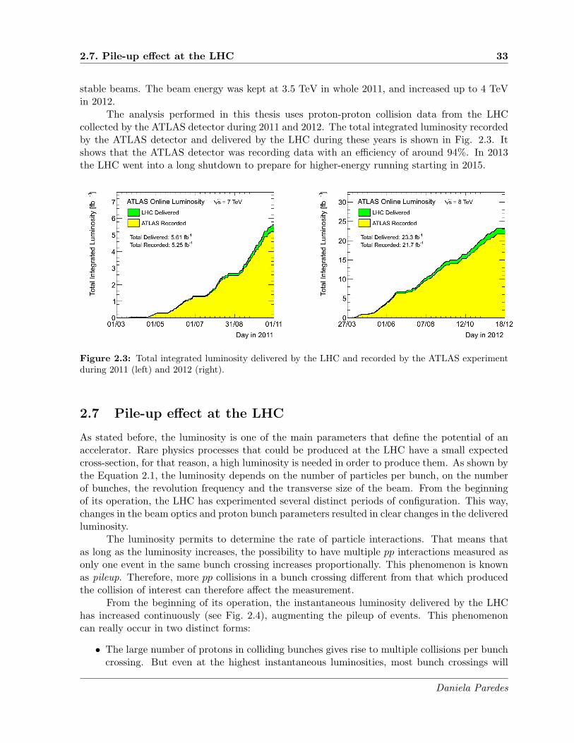
2.7. Pile-up effect at the LHC 33
stable beams. The beam energy was kept at 3.5 TeV in whole 2011, and increased up to 4 TeVin 2012.
The analysis performed in this thesis uses proton-proton collision data from the LHCcollected by the ATLAS detector during 2011 and 2012. The total integrated luminosity recordedby the ATLAS detector and delivered by the LHC during these years is shown in Fig. 2.3. Itshows that the ATLAS detector was recording data with an efficiency of around 94%. In 2013the LHC went into a long shutdown to prepare for higher-energy running starting in 2015.
Figure 2.3: Total integrated luminosity delivered by the LHC and recorded by the ATLAS experimentduring 2011 (left) and 2012 (right).
2.7 Pile-up effect at the LHC
As stated before, the luminosity is one of the main parameters that define the potential of anaccelerator. Rare physics processes that could be produced at the LHC have a small expectedcross-section, for that reason, a high luminosity is needed in order to produce them. As shown bythe Equation 2.1, the luminosity depends on the number of particles per bunch, on the numberof bunches, the revolution frequency and the transverse size of the beam. From the beginningof its operation, the LHC has experimented several distinct periods of configuration. This way,changes in the beam optics and proton bunch parameters resulted in clear changes in the deliveredluminosity.
The luminosity permits to determine the rate of particle interactions. That means thatas long as the luminosity increases, the possibility to have multiple pp interactions measured asonly one event in the same bunch crossing increases proportionally. This phenomenon is knownas pileup. Therefore, more pp collisions in a bunch crossing different from that which producedthe collision of interest can therefore affect the measurement.
From the beginning of its operation, the instantaneous luminosity delivered by the LHChas increased continuously (see Fig. 2.4), augmenting the pileup of events. This phenomenoncan really occur in two distinct forms:
• The large number of protons in colliding bunches gives rise to multiple collisions per bunchcrossing. But even at the highest instantaneous luminosities, most bunch crossings will
Daniela Paredes

34 Chapter 2. The Large Hadron Collider
contain only one hard interaction. Additional interactions in each crossing are referred toas in-time pileup, which typically comes from soft particles, which contribute with energydistributed homogenously throughout the detector. The best estimator of the in-timepileup is the number of reconstructed primary vertices.
• Though only one pp interaction happened in a given bunch crossing, pp interactions in aprevious bunch crossing can also affect the measurement if the spacing between the bunchesis shorter than the response time of the detectors. This way, additional collisions fromdifferent bunches are recorded simultaneously. This is referred to as out-of-time pileup,and it will become important as the LHC bunch spacing is decreased. The out-of-timepileup is estimated using the average number of pp collisions per bunch crossing at thetime of the recorded event3.
Month in 2010 Month in 2011 Month in 2012Jan Apr Jul
Oct Jan Apr JulOct Jan Apr Jul
Oct
]-1
s-2
cm
33
Pe
ak L
um
ino
sity [
10
0
2
4
6
8
10 = 7 TeVs = 7 TeVs = 8 TeVs
ATLASOnline Luminosity
Figure 2.4: The peak instantaneous luminosity delivered to ATLAS per day versus time during the ppruns of 2010, 2011 and 2012.
In 2010, the maximum instantaneous luminosity delivered by the LHC was about 2.1 ×1032cm−2s−1, and the bunch spacing was not smaller than 150 ns. In this low-luminosity runningconditions, the average number of interactions per event was 2.2, with a maximum of 3.78, mostlyarising from in-time pileup. The effect of the out-of-time pileup was small due to the big bunchspacing. In 2011, the bunch spacing was reduced to 50 ns with an instantaneous luminosity thatreached values of 3.65× 1033cm−2s−1 increasing the out-of-time pileup. The average number ofpp collisions per bunch crossing was between 3 and 8 until September technical stop, with anaverage of 6.3. It increased to reach values between 5 and 17 after that September, with anaverage of 11.6. In 2012, the bunch spacing was kept to 50 ns, and the luminosity reached avalue of 7.73×1033cm−2s−1 with a mean number of interactions per bunch crossing of 20.7. Themaximum mean number of events per beam crossing versus day during the pp collisions runs of2010, 2011 and 2012 is shown in Fig. 2.5. At the design luminosity and for a bunch spacing of25 ns, it is expected to have around 23 interactions per bunch crossing.
3This number is computed using the average luminosity over a time period ∆t ≫ 600 ns, the total inelastic ppcross-section, the LHC revolution frequency and the number of colliding bunches.
Daniela Paredes

2.7. Pile-up effect at the LHC 35
Month in 2010 Month in 2011 Month in 2012Jan Apr Jul
Oct Jan Apr JulOct Jan Apr Jul
Oct
Pe
ak in
tera
ctio
ns p
er
cro
ssin
g
0
5
10
15
20
25
30
35
40
45
50
= 7 TeVs = 7 TeVs = 8 TeVs
ATLASOnline Luminosity
Figure 2.5: Maximum mean number of events per beam crossing versus day during the pp collisionsruns of 2010, 2011 and 2012.
Daniela Paredes

36 Chapter 2. The Large Hadron Collider
Daniela Paredes
Chapter 3
The ATLAS detector
Contents
3.1 Introduction . . . . . . . . . . . . . . . . . . . . . . . . . . . . . . . . . . . . . 38
3.2 The coordinate system and basic quantities . . . . . . . . . . . . . . . . . . 39
3.3 Inner detector . . . . . . . . . . . . . . . . . . . . . . . . . . . . . . . . . . . . 40
3.3.1 The Pixel Detector . . . . . . . . . . . . . . . . . . . . . . . . . . . . . . . . . . 41
3.3.2 The SemiConductor Tracker . . . . . . . . . . . . . . . . . . . . . . . . . . . . . 42
3.3.3 The Transition Radiation Tracker . . . . . . . . . . . . . . . . . . . . . . . . . 44
3.4 Calorimeters . . . . . . . . . . . . . . . . . . . . . . . . . . . . . . . . . . . . . 45
3.4.1 The electromagnetic calorimeter . . . . . . . . . . . . . . . . . . . . . . . . . . 47
3.4.2 The hadronic calorimeter . . . . . . . . . . . . . . . . . . . . . . . . . . . . . . 49
3.4.3 The LAr forward calorimeter . . . . . . . . . . . . . . . . . . . . . . . . . . . . 52
3.5 Muon spectrometer . . . . . . . . . . . . . . . . . . . . . . . . . . . . . . . . . 53
3.5.1 The high-precision tracking chambers . . . . . . . . . . . . . . . . . . . . . . . 55
3.5.2 The trigger chambers . . . . . . . . . . . . . . . . . . . . . . . . . . . . . . . . 56
3.6 Forward detectors . . . . . . . . . . . . . . . . . . . . . . . . . . . . . . . . . . 58
3.6.1 The MBTS . . . . . . . . . . . . . . . . . . . . . . . . . . . . . . . . . . . . . . 58
3.6.2 The LUCID detector . . . . . . . . . . . . . . . . . . . . . . . . . . . . . . . . . 59
3.6.3 The ZDC . . . . . . . . . . . . . . . . . . . . . . . . . . . . . . . . . . . . . . . 59
3.6.4 The ALFA detector . . . . . . . . . . . . . . . . . . . . . . . . . . . . . . . . . 59
3.7 Magnet system . . . . . . . . . . . . . . . . . . . . . . . . . . . . . . . . . . . . 60
3.7.1 The solenoid magnet . . . . . . . . . . . . . . . . . . . . . . . . . . . . . . . . . 60
3.7.2 The toroidal magnet system . . . . . . . . . . . . . . . . . . . . . . . . . . . . . 61
3.8 The trigger and data acquisition system (TDAQ) . . . . . . . . . . . . . . . 61
3.8.1 The Level-1 trigger . . . . . . . . . . . . . . . . . . . . . . . . . . . . . . . . . . 62
3.8.2 The Level-2 trigger . . . . . . . . . . . . . . . . . . . . . . . . . . . . . . . . . . 63
3.8.3 The Event Filter . . . . . . . . . . . . . . . . . . . . . . . . . . . . . . . . . . . 63
Daniela Paredes

38 Chapter 3. The ATLAS detector
3.1 Introduction
The ATLAS experiment was proposed in 1994 and approved in 1996. Currently this experimentgroups more than 3000 scientists from 175 institutions in 38 countries, making it one of thelargest collaborations ever formed in the world.
As mentioned in the previous chapter, ATLAS is one of the general purpose detectorsconstructed at the LHC, designed to improve or confirm measurements of the Standard Modeland to look for New Physics. It is 45 m long, 25 m in diameter and weighs about 7000 tons. Itsdesign requirements were driven by some of the most important signals for possible New Physicswhich could be observed, and to support the hard radiation environment.
The ATLAS detector consists of an ensemble of sub-detectors with cylindric shape placedaround the interaction point where the proton beams from the LHC collide. From the interactionpoint outwards, these sub-detectors can be identified as: the inner detector, which is used fortracking of charged particles, the calorimeters, which surround the inner detector and are usedfor measuring the energies of the particles traversing them, and the muon spectrometer, whichis the most external system and is used for identifying muons and measuring their momenta. Amagnet system is used to bend the charged particles for momentum measurement. The overallATLAS detector layout is shown in Fig. 3.1. Additional measurements can be done using theforward detectors. The detector has been designed as hermetic as possible, meaning that it mustdetect all particles produced with the exception of neutrinos. However, the neutrinos presencecan be inferred by measuring a momentum imbalance among detected particles.
A trigger system has also been implemented, which has been designed to decide whichevents should be recorded in a very short time. Each aspect already mentioned will be discussedin this chapter, starting from a definition of the coordinate system and the basic quantities usedin this thesis.
Figure 3.1: The Atlas detector.
Daniela Paredes

3.2. The coordinate system and basic quantities 39
3.2 The coordinate system and basic quantities
The coordinate system used to describe the ATLAS detector and the particles emerging fromthe collisions defines the origin at the nominal proton-proton interaction point, located in thegeometrical center of the detector. The reference system is a Cartesian right-handed coordinatesystem, where the counter-clockwise beam direction defines the positive z-axis. The x-y plane isperpendicular to the z-axis, with the positive x-axis pointing from the interaction point to thecenter of the LHC ring and the y-axis points towards the surface, upwards from the interactionpoint. The detector is symmetric for positive and negative z, the part of the detector corres-ponding to z > 0 is called “Side A”, while for z < 0 is called “Side C”. Some subsystems of thedetector are composed of a barrel portion with detecting elements parallel to the z-axis, and twoendcap portions with detecting elements arranged in transversal planes to the beam axis. Theseendcaps can be referred as “Endcap-A” and “Endcap-C”.
From this reference system, cylindrical and polar coordinates are defined in order to descri-be either the detecting elements, the trajectories of the particles through the detector, or some ofthe variables repeatedly used throughout this thesis. The azimuthal angle φ is measured in thex-y plane around the beam axis (φ = 0 is defined along the positive x-axis), while the polar angleθ is taken with respect to the positive z direction. The radius r is defined as the perpendiculardistance to the z axis.
In proton-proton collisions, the constituents partons carry unknown fractions of the protonmomentum. A large fraction of the longitudinal momentum (z-axis) gives rise to hard processeswhich cannot be fully measured, and some of this momentum is lost in the remnants that escapedown the beam pipe, thus the overall boost of the collision is unknown. For that reason, Lorentzinvariant quantities are used in most analyses. Thus, the polar angle is rarely used and it isreplaced by the rapidity
y =1
2ln[(E + pz)/(E − pz)], (3.1)
with E representing the energy of the object, and pz its momentum along the beam direction; orrather the pseudorapidity, which is equal to the rapidity in the ultrarelativistic approximation
η = − ln[tan(θ/2)]. (3.2)
Since η is a function only of the polar angle θ, it has a well-defined and mass-independentinterpretation in the laboratory frame. It is also common to refer to the η-φ angle space, inwhich the surfaces of the cylindrical detectors appear as flat sheets, and where the ∆R cone isdefined as
∆R =√
∆η2 +∆φ2. (3.3)
In proton collisions, partons carry unknown fractions of the proton momentum. Some ofthat momentum is exchanged in the hard interaction, and some of it is lost to remnants thatescape down the beam pipe. This way, the total momentum conservation can not be easilyused to place constraints on the kinematics of an event. However, as protons approach eachother with trajectories that are nearly along the z-axis, momentum is conserved in the planeperpendicular to the beam axis. Thus, in many cases, only the transverse component is usedwhen describing object kinematics, as for example, ET = E sin θ and pT = p sin θ, which aredefined in the x-y plane. In this thesis, the pseudorapidity and the transverse components ofthe energy and momentum, are the kinematic variables which play a fundamental role in theanalysis description.
Daniela Paredes

40 Chapter 3. The ATLAS detector
3.3 Inner detector
The inner detector (ID) [94, 95] is the component of the ATLAS detector closest to the beam axis.It is designed to reconstruct the trajectories of charged particles traversing it, to provide excellentmomentum resolution, and both primary and secondary vertex measurements for charged trackswith a pT > 0.5 GeV1 covering the region |η| < 2.5 with full coverage in φ. It has a transversemomentum resolution σpT/pT = 0.05%pT GeV ⊕ 1%, and it also permits to identify electronswithin |η| < 2.0 for energies between 0.5 GeV and 150 GeV [4].
The inner detector is contained within a cylinder envelope ±3512 mm in length, with outerradius 1150 mm. It is immersed in a 2 T magnetic field generated by a superconducting solenoidmagnet (described in Section 3.7.1), which is necessary to bend charged particles for momentummeasurements2.
Figure 3.2: Cut-away view of the ATLAS inner detector showing each one of the sub-detectors.
In the collisions, a large amount of particles are created in the interaction point generatinga large track density in the detector. In this way, a fine granularity of this part of the detector isneeded. This is managed by means of the use of three high precision subsystems within the innerdetector: the Pixel Detector (Pixel), which is the subsystem closest to the interaction point andis composed of silicon pixel sensors; the SemiConductor Tracker (SCT), which is just outside ofthe pixel detector; and the Transition Radiation Tracker (TRT), which is the outermost system.Their configuration is illustrated in Fig. 3.2. The first two sub-detectors (Pixel and SCT) usesemiconductor technology and provide a small number of hits on track, while the TRT usessmall drift tubes (straw tubes) providing a semi-continuous tracking out to large radii and theidentification/separation of electrons and pions. Each of the sub-detectors is divided in a barrelregion, where they are arranged in concentric cylinders around the beam line (see Fig. 3.3(a));and an endcap region, where the detecting elements are mounted on disks orthogonal to the
1This value is nominal, but it can be as low as 0.1 GeV in some studies of measurements with minimum-biasevents.
2The transverse momentum of the particle is determined by using the following relation pT[GeV] = 0.3×B[T]×R[m], where B is the magnetic field and R the bending radius [96].
Daniela Paredes

3.3. Inner detector 41
beam axis (Fig. 3.3(b)), and which are used to increase the detector coverage in η without asignificant increase in detector surface.
(a) ID Barrel (b) ID Endcap
Figure 3.3: The barrel (a) and endcap (b) tracking system of the ATLAS inner detector. The barrels ofeach sub-detector are arrayed in concentric cylinders around the beam line, while the endcaps are mountedon disks perpendicular to it.
Since all material between the interaction point and the calorimeters degrade the resolutionof the measured energy, the three sub-detectors have to be designed with a structure so that itminimizes the quantity of matter to be crossed by the particles, and also to support the high-radiation conditions to which they are subjected for being the part of the detecter closest to thebeam axis.
In this section, a brief description of each one of the subsystems of the inner detector isgiven. More details about the inner detector can be found in [94, 95].
3.3.1 The Pixel Detector
The innermost tracking subsystem of the ID is the semiconductor pixel detector [97]. It hasthe highest granularity detecting elements as close to the interaction point as possible, whichprovide the most accurate position measurements in ATLAS. The pixel detector consists of threeconcentric barrel layers3 (called ID layers 0-2) placed at radii of 50.5, 88.5, and 122.5 mm aroundthe beam axis covering the central region up to |η| = 1.9; and three endcap disks placed at |z|positions of 495, 580 and 650 mm in each direction along the beam axis from the interactionpoint, extending the total coverage out to |η| = 2.5. This configuration is shown in Fig. 3.4.
Each layer or disk is segmented in modules, which form the basic unit of data acquisition.Each module has an active surface of 6.08×1.64 cm2 and it is assembled primarily of a siliconsensor and 16 radiation-hard front-end chips [98] bump-bonded to the sensor, each with 2880read-out channels, making the only mechanical connection between the sensors and the front-endelectronics. Thus the pixel detector consists of 1744 sensor tiles of approximately 250 µm thickand external dimensions of 19×63 mm2, using oxygenated n-type wafers with readout pixels on
3The innermost one –ID layer 0– is mechanically integrated with the beryllium beam pipe in order to providethe best possible vertex resolution, and it is also called b-layer due to its function in identifying b-quarks initiatedjets.
Daniela Paredes

42 Chapter 3. The ATLAS detector
Figure 3.4: A schematic view of the active region of the pixel detector consisting of barrel and end caplayers.
the n+-implanted side of the detector4. Each sensor tile contains 47232 bipolar diodes (or pixels),but for reasons of space there are four ganged pixels in each column of the front-end chip, leadingto a 46080 readout channels, resulting in a total of 80.4 million pixels. The nominal pixel size is50×400 µm2 and it is dictated by the readout pitch of the front-end electronics5.
A bias voltage is applied to the doped silicon sensors. This way, when a charged particletraverses the semiconductor, the electron-hole pairs created travel to the surface and producethe signal, which is collected if it exceeds a tunable threshold6. A charged particle originated atthe interaction point typically traverses three layers, producing three pixel hits and permittingtherefore determining the particle’s position. The pixel detector is the most important detectorused in the identification and reconstruction of secondary vertices from the decay of, for example,particles containing a b-quark or for b-tagging of jets. Moreover, it provides excellent spatialresolution for reconstructing primary vertices even in the presence of the multiple interactions inproton-proton collisions at the LHC design luminosity. Its intrinsic spatial resolution is 10 µm(r-φ) and 115 µm (z) in the barrel, and 10 µm (r-φ) and 115 µm (r) in the disks.
The pixel modules operate at a nominal voltage between 150 V and 600 V, which increaseswith their exposure to radiation. In order to reduce damage to the sensors due to the radiation,the silicon sensors must be kept at low temperature, between -5◦C and -10◦C. A more detaileddescription about the pixel electronic system is found in [97, 99].
3.3.2 The SemiConductor Tracker
The SCT [100] is located after the pixel detector, forming the middle part of the inner detectorand it is based upon silicon microstrip detector technology. Similarly to the pixel detector, itis composed of a barrel and two endcap sections. The barrel has four coaxial cylindrical layers(called ID layers 3-6) at radii 299, 371, 443, and 514 mm around the beam axis in the radialdirection, covering the central region up to |η| = 1.1. Each endcap region has nine disks of
4Highly oxygenated material increases the tolerance to the radiation to charged hadrons, while the n+ implantsallow the detector to work with good charge-collection efficiency.
5This size is for around 90% of the pixels, for the remaining ones the size is 50×600 µm2 in the regions at thefront-end chips on a module.
6This threshold was set at 3.5 ke− during the 2010 run.
Daniela Paredes

3.3. Inner detector 43
different sizes located between 854 and 2720 mm from the interaction point along the beam axis,providing a total coverage out to |η| = 2.5.
The detector is segmented in 4088 modules: 2112 of rectangular shape in the barrel and1976 trapezoidal in the endcap region. They are illustrated in Fig. 3.5 and 3.6, respectively. Themodules are made of silicon-strip devices that arrange the strips parallel to the beam axis in thebarrel and radially in the endcap, thus providing a precision measurement in (r-φ). They covera total surface of 63 m2 of silicon and provide almost hermetic coverage. The modules consist ofone or two pairs of single-sided p-in-n microstrip sensors glued back-to-back at a 40 mrad stereoangle7. The sensors are divided into 768 AC-coupled strips (there are 1536 strips per module)of 12 cm in length, with a constant pitch of 80 µm in the barrel, while in the endcap it variesfrom 56.9 to 94.2 µm due to the trapezoidal shape. The intrinsic accuracies per module are 17µm (r-φ) and 580 µm (z) in the barrel and 17 µm (r-φ) with 580 µm (r) for the endcap disks.
Figure 3.5: An SCT barrel module [101].
Many of the design considerations of this sub-detector, including the detection principle,are similar to those of the pixel detector. A charged particle originating from the interactionpoint typically crosses eight strip sensors, combining to form four space-point measurements, andcontributing to the measurement of momentum, impact parameter and vertex position. A hit isregistered only if the pulse height exceeds a preset threshold, which normally corresponds to acharge of 1 fC. The charge measured in the strip is stored for a period of ∼3.2 µs and used fortracking if the trigger indicates that the event should be considered in more detail. Each moduleis read out by means of 12 identical 128-channel front-end ASICs8, resulting approximately in6.3 million readout channels [102].
The SCT operates under similar environmental conditions as the pixel detector, sharingthe cooling system (based on C3F8) with it. The nominal voltage in the modules varies from∼150 V (bias voltage) up to 350 V during operation, but it can increase as much as 500 V asradiation damage accumulates. The SCT has been fully operational throughout all data taking
7This configuration gives the required space-point resolution in (r-φ) and r.8Application-Specific Integrated Circuit.
Daniela Paredes

44 Chapter 3. The ATLAS detector
Figure 3.6: One of the types of SCT endcap modules [101].
periods, delivering high quality tracking data for 99.9% (2010), 99.6% (2011) and 99.3% (2012)of the delivered luminosity [103].
3.3.3 The Transition Radiation Tracker
The TRT surrounds the silicon detectors being therefore the outermost part of the inner detector.Its basic detector elements are polyimide drift tubes of 4 mm diameter denoted as straw tubes,filled with a gaseous mixture of 70% Xe, 27% CO2 and 3% O2, and mechanichally stabilized usingcarbon fibers. The straw tube wall was developed in order to have a minimal wall thickness,and specially good electrical and mechanical properties. Each tube is equipped with a 31 µmdiameter tungsten wire plated with 0.5-0.7 µm gold. The wire is going through the center of thestraw, supported at the straw end by an end-plug and it is directly connected to the front-endelectronics.
As the other two sub-detectors, the TRT is composed of a barrel and two endcap sections.The barrel contains 73 layers of straws interleaved with polypropylene fibers forming an approx-imately uniform array parallel to the beam direction, with an average spacing of about 6.6 mmbetween centers radially and tangentially. It is divided into 96 modules of three types, arrangedin three cylinders of 32 modules each one. The barrel spans the radius range from 56 cm up to108 cm and has a sensitivity region of 144 cm in length along the beam axis, covering the regionup to |η| < 1 [104]. Along the z-axis in each endcap there are 160 radial straw planes interleavedwith polypropylene radiator foils9, forming a uniform array in the azimuthal plane perpendicularto the beam axis, covering the backward and forward pseudorapidity region 1 < |η| < 2. In theendcap region, the modules are referred as wheels because of their cylindrical shape and radialstraws like spokes. Each endcap consists of two sets of independent wheels perpendicular to the
9The polypropylene radiator foils in the endcap region together with the polypropylene fibers in the barrelconstitute the transition radiation material of the TRT.
Daniela Paredes

3.4. Calorimeters 45
beam direction, the set closer to the interaction point has 12 wheels, each with eight successivelayers spaced 8 mm apart, while the outer set contains eight wheels, also with eight straw layersbut spaced 15 mm apart [105]. There are 52544 straw tubes of 144 cm length in the barrel, whileeach endcap has 122880 straw tubes of 37 cm length, resulting in a total of 298304 straws, readout by 350848 channels of electronics.
Charged particles passing through the straws ionize the gas inside the tube. Because of theelectric field created by the potential difference between the wire acting as the anode, and thewall of the tube playing the role of the cathode10, the liberated electrons move towards the anodeionizing more the atoms in the gas, inducing therefore an avalanche of electrons that amplifiesthe signal at the wire. During normal operation the maximum electron collection time is ∼48 nswith a drift-time accuracy of 130 µm per straw. The straws only provide measurements in thebending plane, and no measurements along the straw direction.
The TRT is designed so that charged particles with pT > 0.5 GeV and |η| < 2.0 crossat least 36 straws, except in the barrel-endcap transition region (0.8 < |η| < 1.0), where thisnumber decreases to at least 22 straws. This large number of tracking points allows almostcontinuous tracking that improves the precision of the momentum measurement. The TRT alsoprovides electron/pion discrimination via transition radiation from the fibers interleaved betweenthe straws in the barrel and the foils in the endcaps. When a relativistic particle pass betweenmedia with different dielectric constants, it emits energy in the form of photons. The total energyradiated by this particle is proportional to its Lorentz γ factor, which will be significantly largerfor an electron with the same energy as a pion11. The emitted photons are absorbed by the Xenongas, which increases the transition radiation and produce stronger signals. The amplitude of thissignal will be higher when an electron traverses the transition material than when a pion does.Transition radiation photons yield much larger signals than minimum-ionizing charged particles.The distinction between transition radiation and tracking signals is obtained by using separatelow and high thresholds in the front-end electronics12. Summarizing, the difference in the signalamplitude allows for particle identification by using transition radiation and tracking by usingits ionization signals.
In contrast with the silicon detectors, the TRT is designed to operate at room temperature,but in order to avoid high-voltage discharges and pollution from diffusion of gas from the outsideinto the straws through their walls, or flush away any gas leakage from inside the straws, themodules have to be operated in an envelope of CO2.
3.4 Calorimeters
The ATLAS calorimeter system is located outside the solenoid magnet that surrounds the innerdetector. It consists of several non-compensating13 sampling calorimeters which use different
10The wires are kept at ground potential, while the walls of the straws are kept at -1530 V to give a gain of2.5× 104 for the chosen gas mixture with 5-10 mbar over-pressure.
11γ = E/mc2, where E is the energy of the particle and m its mass. For an electron with the same energy as apion, the γ factor will be significately larger for an electron due to its mass being around 250 times smaller thanthe pion mass.
12The low-threshold is for ionization signals and it is set at ≈ 250 eV, while the high-threshold is for transitionradiation and it is set at ≈ 6 keV.
13It refers to the fact that some energy released in nuclear collisions is lost to nuclear recoils and dissociationand it is not deposited in the active material.
Daniela Paredes

46 Chapter 3. The ATLAS detector
technologies suited in order to study the different physics processes of interest, and to supportthe hard radiation environment. It has a full φ-symmetry and coverage around the beam axisspanning the pseudorapidity range up to |η| < 4.9, with a varying granularity in η×φ. Samplingcalorimeters use alternating layers of absorber and active material. The incident particle interactswith the material in the calorimeter through several processes (they depend on the particle, itskinematics and the medium) producing a shower of particles that are detected in the activemedium which measures the deposited energy on the material. In general, the absorber mediumis chosen to be a dense material with a high stopping power so that particles in the energy rangeunder study are contained in the calorimeter.
This way, the calorimeter system is designed to stop all the interacting particles emerg-ing from the interaction point (except muons, which are not absorbed by the calorimeters sincethey are highly penetrating particles) measuring their energy and position. It provides electro-magnetic and hadronic energy measurements. Thus, the ATLAS calorimeters can be classifiedcorresponding to their design as electromagnetic and hadronic calorimeters. The electromagnetic(EM) calorimeter has a high granularity, which is needed for precision measurements of elec-trons and photons. It also contributes to measuring the energy of hadrons in jets. The hadroniccalorimeter has a coarser granularity, but it is sufficient to satisfy the hadronic jets reconstructionand missing transverse energy measurements.
There are four calorimeters in ATLAS detector: the Liquid Argon (LAr) electromagneticcalorimeter, which covers the pseudorapidity region up to |η| < 3.2, the Tile hadronic calorimetercovering |η| < 1.7, the LAr hadronic endcap calorimeters covering 1.5 < |η| < 3.2, and the LArForward calorimeter covering the region 3.1 < |η| < 4.9. The overall system is depicted inFig. 3.7, which indicates where the various calorimeters are installed. The ones closest tothe interaction point are accommodated in three cryostats: one barrel and two endcaps. Thebarrel contains the LAr electromagnetic barrel calorimeter (EMB), while each one of the twoendcap cryostats contains a LAr electromagnetic endcap (EMEC), a LAr hadronic endcap (HEC),situated behind the EMEC, and a forward calorimeter (FCal) covering the region closest to thebeam axis. In all these calorimeters the active medium is liquid argon. The showers in the argonliberate electrons that are later collected and recorded. Liquid argon was chosen as the activemedium due to its resistance to radiation, its linear behavior and its stability of response. TheLAr calorimeters are housed in cryostats, which are cooled to a temperature of ∼89 K in order tomaintain the argon in liquid state. Over the pseudorapidity range |η| < 1.8, the EM calorimeteris preceded by a presampler detector, which is installed behind the cryostat, and it is used tocorrect for the energy lost in the material upstream of the calorimeter [4].
The outer section of the calorimeter system is constituted by the Tile calorimeter. Itconsists of iron plates used as absorber material and scintillating plastic tiles used as activemedium. Hadronic showers developing in the plates illuminate the tiles, the light thus producedis detected and recorded.
Hadronic and EM calorimeters provide separate event data for reconstruction. But, dueto the fact that some energy can be deposited in the inactive region of the detector, they donot manage to measure the full energy of the original particle. The response of the calorimetertherefore refers to the fraction of energy of the incident particle that is measured. For thatreason, calibrations need to be applied in order to properly measure the energy of the originalparticle.
In this section, a brief description of the electromagnetic and hadronic calorimeters is given.More information about the calorimeter system can be found in [4, 106, 107].
Daniela Paredes

3.4. Calorimeters 47
Figure 3.7: Cut-away view of the ATLAS calorimeter system. Calorimeters with LAr as active mediumare situated in the inner section, while in the outer section the sampling medium consists of scintillatortiles [4].
3.4.1 The electromagnetic calorimeter
The EM calorimeter [108] provides precision measurements of electrons and photons, contributingalso to measuring the energy of hadrons in jets. It is a lead-LAr detector with accordion-shapedkapton electrodes and lead absorber plates. The LAr is used as the active medium. The accordiongeometry provides a full coverage in φ without azimuthal cracks, and a fast extraction of thesignal at the rear or at the front of the electrodes. When a photon traverses the calorimeter,it interacts with the lead and produces an electron-positron pair. This pair also interacts withthe material, producing Bremsstrahlung photons, which have the same effect that the incidentphoton creating an electromagnetic shower. Charged particles that traverse the active materialionize it, releasing ionization electrons which are collected as a current in the presence of anelectric field by the electrodes mounted on the accordion plates. An electron passing throughthe LAr will produce the same reaction chain as a photon.
The accordion geometry of this calorimeter also allows it to have several active layers indepth. Thus the EM calorimeter is segmented in three longitudinal layers for the region up to|η| < 2.5. The first layer (at lowest r) is equipped with narrow strips in η with a pitch of ∼4 mm,and it has a depth of ∼6 radiation lengths (X0) including dead material and presampler. It acts asa preshower detector, helping to identify particles and providing a precise position measurementin η. Only a small fraction of the energy of a particle is deposited there. The second (middle)layer is transversally segmented into square towers (∆η×∆φ = 0.25×0.25, ∼4×4 cm2 at η = 0),with a total thickness of the calorimeter up to the end of this section of ∼24X0. Most of theenergy is deposited in this layer. The last layer has a coarser granularity in η (twice with respectto the previous section), with a thickness between 2X0 and 12X0, and only contains the tailsof the electromagnetic showers. For the region covering |η| > 2.5, the calorimeter is segmented
Daniela Paredes

48 Chapter 3. The ATLAS detector
in two longitudinal layers, with a coarser lateral granularity than for the rest of the acceptance.The cells in the calorimeter point towards the interaction point over the complete η-coverage.As said before, the EM calorimeter is preceded by a presampler detector, installed behind thecryostat in the region where the amount of material exceeds ∼2X0, corresponding to |η| < 1.8. Itconsists of an active LAr layer of thickness 1.1 cm in the barrel and 0.5 cm in the endcap region.At the transition between the barrel and the endcap EM calorimeters, it is complemented by ascintillator slab inserted in the crack between the barrel and endcap cryostats. The presampler isdesigned to estimate and correct for losses of energy by electrons and photons through a particle’sinteraction with material upstream of the calorimeter. A large amount of material is situatedin front of the EM calorimeter in the region 1.37 < |η| < 1.52, for that reason, electrons andphotons that fall within this region have reduced energy and position resolutions, and thereforeare excluded in the analysis [107].
The EM calorimeter is divided into a barrel part covering the region up to |η| < 1.475and two endcap components covering 1.375 < |η| < 3.2, each housed in their own cryostat. Theabsorbers in the barrel have a thickness of 1.53 mm for |η| < 0.8 and 1.13 mm for |η| > 0.8, whilein the endcaps their thickness is 1.7 mm for |η| < 2.5 and 2.2 mm for |η| > 2.5. The electrodesare located in the gaps between the lead absorbers, and consists of three copper layers, whichare separated by insulating polyimide sheets. The inner layer is used to read out the signal bymeans of capacitive coupling, while the two outer ones are at high-voltage potential. As can beinferred, the LAr is located also in the gaps between the absorbers.
The full barrel cryostat is 6.8 m long, with an outer radius of 2.25 m, and an inner cavityradius of 1.15 m. The barrel consists of two identical half-barrels, separated by a gap of 4 mmat z = 0 [4]. The length of each barrel is 3.2 m along the z-axis, with an inner diameter of2.8 m and an outer one of 4 m. Each half-barrel weighs around 57 tonnes and consists of 1024absorbers, interleaved with readout electrodes. The electrodes are located in the middle of thegap by honeycomb spacers. The size of the drift gap on each side of the electrode is 2.1 mm,which at the nominal operating voltage of 2 kV gives an average drift time of ∼ 450 ns. Eachhalf-barrel is divided into 16 modules. The total thickness of a module is at least 22X0, whichincreases to 30X0 between |η| = 0 and |η| = 0.8, and from 24X0 to 33X0 between |η| = 0.8 and|η|=1.3. One example of a barrel module is shown in Fig. 3.8(a).
Each endcap calorimeter is divided in two coaxial wheels: an outer wheel covering therange 1.375 < |η| < 2.5, and an inner wheel covering 2.5 < |η| < 3.2. The boundary between theinner and the outer wheel (located at |η| = 2.5) is mostly filled with low-density material, and is 3mm wide. It matches the acceptance of the inner detector. Each endcap is housed in its cryostat(which is also shared with the hadronic wheels and the forward calorimeter). An example of anendcap cryostat is shown in Fig. 3.8(b). Each endcap wheel is divided into eight wedge-shapedmodules and contains 768 absorbers interleaved with readout electrodes in the outer wheel and256 absorbers in the inner one. As for the barrel, the electrodes are in the middle of the gaps,and are positioned by honeycomb spacers. The total active thickness of each endcap is greaterthan 24X0 (except for |η| < 1.475), and it increases to 38X0 as |η| increases from 1.475 to 2.5for the outer wheel, and from 26 to 36X0 as |η| increases from 2.5 to 3.2 for the inner wheel.
The fine segmentation of the EM calorimeter allows detailed measurements of electronsand photons. Its energy resolution is σE/E = 10%/
√E ⊕ 0.7% [4].
Daniela Paredes
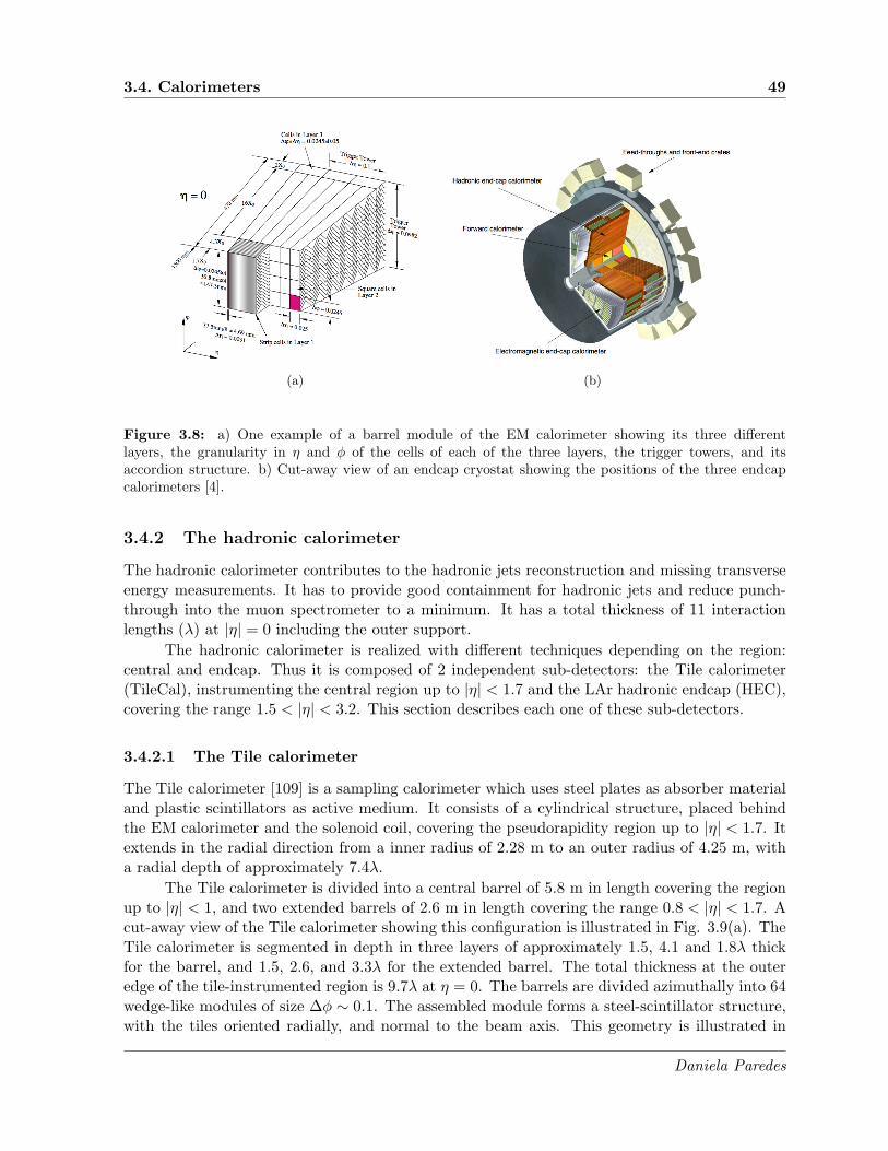
3.4. Calorimeters 49
(a) (b)
Figure 3.8: a) One example of a barrel module of the EM calorimeter showing its three differentlayers, the granularity in η and φ of the cells of each of the three layers, the trigger towers, and itsaccordion structure. b) Cut-away view of an endcap cryostat showing the positions of the three endcapcalorimeters [4].
3.4.2 The hadronic calorimeter
The hadronic calorimeter contributes to the hadronic jets reconstruction and missing transverseenergy measurements. It has to provide good containment for hadronic jets and reduce punch-through into the muon spectrometer to a minimum. It has a total thickness of 11 interactionlengths (λ) at |η| = 0 including the outer support.
The hadronic calorimeter is realized with different techniques depending on the region:central and endcap. Thus it is composed of 2 independent sub-detectors: the Tile calorimeter(TileCal), instrumenting the central region up to |η| < 1.7 and the LAr hadronic endcap (HEC),covering the range 1.5 < |η| < 3.2. This section describes each one of these sub-detectors.
3.4.2.1 The Tile calorimeter
The Tile calorimeter [109] is a sampling calorimeter which uses steel plates as absorber materialand plastic scintillators as active medium. It consists of a cylindrical structure, placed behindthe EM calorimeter and the solenoid coil, covering the pseudorapidity region up to |η| < 1.7. Itextends in the radial direction from a inner radius of 2.28 m to an outer radius of 4.25 m, witha radial depth of approximately 7.4λ.
The Tile calorimeter is divided into a central barrel of 5.8 m in length covering the regionup to |η| < 1, and two extended barrels of 2.6 m in length covering the range 0.8 < |η| < 1.7. Acut-away view of the Tile calorimeter showing this configuration is illustrated in Fig. 3.9(a). TheTile calorimeter is segmented in depth in three layers of approximately 1.5, 4.1 and 1.8λ thickfor the barrel, and 1.5, 2.6, and 3.3λ for the extended barrel. The total thickness at the outeredge of the tile-instrumented region is 9.7λ at η = 0. The barrels are divided azimuthally into 64wedge-like modules of size ∆φ ∼ 0.1. The assembled module forms a steel-scintillator structure,with the tiles oriented radially, and normal to the beam axis. This geometry is illustrated in
Daniela Paredes

50 Chapter 3. The ATLAS detector
Fig. 3.9(b). The gaps between the central barrel and the extended barrels are instrumented withspecial modules which permit partially to recover the energy lost in the crack regions.
(a) (b)
Figure 3.9: a) Cut-away view of the Tile calorimeter. b) Structure of a module of the Tile calorimeter,showing the placement of the scintillator tiles, the steel plates and the readout components [4].
The tiles are 3 mm thick with radial lengths ranging from 97 mm to 187 mm, and azimuthallengths ranging from 200 mm to 400 mm, while the basic element of the absorber structureconsists of a master plate of 5 mm thick, onto which 4 mm thick spacer plates are glued ina staggered way to form the pockets in which the tiles are placed. Hadronic showers crossingthe tiles induce the production of ultraviolet light in the base material (polystyrene). The lightproduced is collected and converted to visible light by wavelength shifting optical fibers, whichare grouped together and coupled to the photomultiplier tubes (PMTs) housed at the outer edgeof each module. The charge collected by each PMT is then digitized and transmitted to theATLAS readout system. This information is reconstructed and summed up in order to measurethe initial particle energy. The tiles orientation together with the fibres readout on the tile edges,permit an almost complete azimuthal coverage. The three-dimensional structure of the readoutcell is defined by the previous fibre grouping, and provides in η an approximately projectivegeometry towards the interaction region. These cells have dimensions ∆η × ∆φ = 0.1 × 0.1 inthe first two layers, and 0.2× 0.1 in the last layer. The segmentation in depth in η of the barreland extended barrels is shown in Fig. 3.10.
The readout electronics is integrated with the mechanical structure. All the front-endelectronics together with the PMTs are mounted in aluminum units (1.4 m long) called drawers,which are placed at the rear of each module.
The Tile calorimeter is essential for measuring the energy and direction of the hadronsproduced in the collisions, and it also complements the energy measurement of the EM calorime-ter for these hadrons. These appear in the detector as isolated hadrons, or jets of charged andneutral particles. The hadronic calorimeter hermeticity allows, in addition, to measure the miss-ing transverse energy and therefore reconstructing particles that are escaping to the detection.
Daniela Paredes

3.4. Calorimeters 51
Figure 3.10: Segmentation in depth in η of the TileCal modules in the central (left) and extended (right)barrels [4].
The Tile calorimeter is also equipped with three hardware calibration systems: Cesium [110],LASER [14], and Charge Injection System [111]. Together, they provide a complete calibrationof the hardware chain, from the active modules to the readout electronics. In particular, theLASER system is studied in Chapter 4.
The energy resolution of the Tile calorimeter is σE/E = 50%/√E ⊕ 3% [4].
3.4.2.2 The LAr hadronic endcap calorimeter
The hadronic calorimetry is extended in the pseudorapidity region 1.5 < |η| < 3.2 by the HEC.This is a copper/LAr sampling calorimeter with a flat-plate design. The copper-plate acts asabsorber, while the LAr does as active medium. LAr is used because of its higher radiationtolerance, which is required for the forward regions. The segmentation of the HEC in η × φ is0.1× 0.1 up to |η| < 2.5, and 0.2× 0.2 for the pseudorapidity region 2.5 < |η| < 3.2.
The HEC consists of two independent wheels per endcap, which are located behind theEMEC sharing the same LAr cryostats. The wheels in each endcap have a cylindrical shapewith an outer radius of 2030 mm, and they are placed one after the other along the beamdirection. The wheels inside the cryostat are supported by two sliding rails, which form part ofthe mechanical structure. Each wheel contains two longitudinal sections (making a total of fourlayers per endcap), and is built of 32 identical wedge-shaped modules. One example of a moduleis shown in Fig. 3.11(a). The modules of the wheels closest to the interaction point are made of24 copper plates of 25 mm thickness, plus a 12.5 mm thick front plate, while in the rear wheels,they are made of 16 plates of 50 mm thickness, plus a 25 mm thick front plate. The inner radiusof the copper plates is 475 mm, except in the overlap region with the forward calorimeter wherethis radius becomes 372 mm. The copper plates are interleaved with 8.5 mm LAr gaps. Thesegaps are divided by three parallel electrodes into four separate drift zones of about 1.8 mm, asshown is Fig. 3.11(b). The middle electrode serves as the readout electrode and defines thelateral (η × φ) segmentation, while to the other two electrodes a high voltage is applied. Thetypical drift time for electrons in the drift zone is ∼430 ns for a nominal voltage of 1800 V.
Daniela Paredes

52 Chapter 3. The ATLAS detector
The HEC overlaps with the forward calorimeter in the range 3.1 < |η| < 3.2, and withthe Tile calorimeter in the region 1.5 < |η| < 1.7. Its energy resolution is the same as the Tilecalorimeter.
(a) (b)
Figure 3.11: a) Cut-away view of a HEC module. b) Arrangement of the HEC readout structure in aLAr gap [4].
3.4.3 The LAr forward calorimeter
The LAr forward calorimeter (FCal) consists of two cylindrical endcaps, with a front face placedat a distance of approximately 4.7 m from the interaction point along the beam axis. It uses LAras the active medium covering the pseudorapidity region 3.1 < |η| < 4.9. As mentioned before,it is integrated into the same cryostat as the endcap calorimeters.
The FCal has to accommodate at least 9λ of active detector in a short longitudinal space,and therefore making it a high density detector. Each FCal endcap is divided into three 45 cmdeep modules: one electromagnetic and two hadronics. This configuration is illustrated inFig. 3.12(a). The electromagnetic module is the closest to the interaction point, and in or-der to optimize the resolution, uses copper as absorber material. The hadronic modules are faraway, and use tungsten as the absorber medium to limit the extension of the particle shower.In each module, the calorimeter consists of a metal matrix with regularly spaced longitudinalchannels filled with the electrode structure, which consists of concentric rods centered in tubesparallel to the beam direction. One example of this arrangement for one hadronic module isshown in Fig. 3.12(b). LAr fills the gap between the rod and matrix. These gaps are 250 µmwide in the first module (electromagnetic module) and 375 (500) µm in the second (last) one(hadronic modules). These small LAr gaps are needed due to the high radiation environment inthis region of the detector, also in order to avoid ion build-up problems and to provide at the
Daniela Paredes

3.5. Muon spectrometer 53
same time the highest possible density. They lead to a faster signal, with a drift time of 60 nsfor the electromagnetic module, while for the hadronic ones it scales with the gap size. The rodsare at positive high voltage while the tubes and matrix are grounded.
(a) (b)
Figure 3.12: a) Diagram showing the modules located in one endcap cryostat. The structural parts ofthe cryostat are shown in black. b) View of the FCal hadronic module absorber matrix [4].
The FCal provides uniformity coverage to the calorimeter, reducing the effects of the crackand dead space in the transition region (around |η| = 3.1). A shielding plug made of copper alloylocated behind the last hadronic module reduces the radiation background levels to the muonspectrometer. Signals are read out through the front of the electromagnetic module and throughthe back of the two hadronic modules. The total number of readout channels is 3524. Its energyresolution is σE/E = 100%/
√E ⊕ 10% [4].
3.5 Muon spectrometer
The Muon Spectrometer (MS) [112] is the outermost part of the ATLAS detector. It is designedto detect charged particles which manage to traverse the calorimeters, and to measure theirmomentum in the range |η| < 2.7. The MS allows identification of muons with momenta above 3GeV, and the measurement of their momenta with a resolution between 3% and 4% for a rangeof 10 GeV < pT < 500 GeV and better than 10% for pT’s up to 1 TeV [113]. It is based on themagnetic deflection of muon tracks in the large superconducting air-core toroid magnets, whichprovides between 1 and 7.5 Tm of bending power. The magnetic field necessary to bend theparticle trajectories in the pseudorapidity range up to |η| < 1.4 is provided by the large barreltoroid, while in the region 1.6 < |η| < 2.7 muon tracks are bent by the smaller endcap magnetsplaced in both extremes of the barrel toroid. A combination of the barrel and endcap fieldsprovides the magnetic deflection in the transition region 1.4 < |η| < 1.6. The magnetic fieldprovided by this magnet configuration is mostly orthogonal to the muon trajectories, minimizingthe degradation of resolution due to the multiple scattering. The requirements to measure thecurvature of high-pT tracks dictate the size of the MS, and therefore also the dimensions of theATLAS detector.
The MS is also designed to trigger on these particles traversing the calorimeters in thepseudorapidity region up to |η| < 2.4. It is instrumented with separate trigger and high-precision
Daniela Paredes

54 Chapter 3. The ATLAS detector
tracking chambers. The chambers are arranged such that particles emerging from the interactionpoint can traverse three stations of chambers, which are situated so that they provide goodhermeticity and optimum momentum resolution.
As for the other detectors in ATLAS, the MS is formed by a barrel and two endcap regions.The barrel chambers form three cylinders concentric with the beam direction, placed at radii ofapproximately 5 m, 7.5 m, and 10 m away from the beam, covering the pseudorapidity range upto |η| < 1. The chambers in the barrel are of rectangular shape with size of 2-10 m2. In the twoendcap regions, the chambers are arranged in four disks, located at |z| ≈ 7.4 m, 10.8 m, 14 m,and 21.5 m from the interaction point, and concentric with the beam axis, covering the range1 < |η| < 2.7. The most of the endcap chambers are of trapezoidal shape with sizes ranging from1-10 m2. All chambers combined provide an almost full coverage, except in the region with η ≈ 0,where a gap in the chamber coverage has been left open for the passage of cables and services ofthe inner detector, central solenoid, and the calorimeters. A 16-fold azimuthal segmentation hasbeen chosen for both, the barrel and endcaps, which follows the eightfold azimuthal symmetry ofthe magnet structure. The chambers are arranged in small and large sectors. The small sectorscover the azimuthal range around the barrel toroid coils, while the large sectors cover the regionbetween them. The barrel toroid structure supports all the barrel chambers and a part of theendcap chambers. The rest of the endcap chambers are supported on the service structures atthe extremes of the experimental hall, and on special support frames.
The MS is equipped with four different kind of chambers: Monitored Drift Tube cham-bers (MDT), Cathode Strip Chambers (CSC), Resistive Plate Chambers (RPC) and Thin GapChambers (TGC). The first two are used for precision measurements of muon tracks, while theother two are used for the trigger and data acquisition system. They are illustrated in Fig. 3.13.The muon chambers are described in this section according to their function. Thus we havehigh-precision tracking chambers and trigger chambers.
Figure 3.13: Cut-away view of the muon spectrometer showing the positions of the four different kindof chambers [4].
Daniela Paredes

3.5. Muon spectrometer 55
3.5.1 The high-precision tracking chambers
The tracking precision chambers determine the muon momenta from the deflection of the muontracks in the magnetic field. They are built out of two kind of technologies: MDT and CSC. TheMDT chambers perform the measurement of the muon trajectory up to |η| < 2.7, except in theforward region closest to the interaction point, where their coverage is limited up to |η| < 2. Inthis region, the particle fluxes and muon-track density are the highest and therefore the MDTchambers are replaced by CSC with higher granularity. The CSC cover the range 2 < |η| < 2.7,and are used to sustain the demanding rate and background conditions in this region of thedetector. The precision measurement of the muon tracks is made in the r-z projection, in adirection parallel to the bending direction of the magnetic field. The z coordinate is measuredin the barrel, while the radial coordinate r is measured in the transition and endcap regions. Ameasurement of φ is also obtained by the CSC in the forward region.
The basic detection elements of the MDT chambers are pressurized aluminium drift tubesof 29.97 mm diameter and 400 µm wall thickness, with a 50 µm diameter central gold-platedW-Re wire. The wire is at a potential of 3080 V, and is held in position at the tube ends by acylindrical end-plug, which guarantees the concentricity of the wire. The HV supply system andthe signal transmission to the electronics are located at opposite ends. The tubes are operatedwith Ar/CO2 gas (93/7) at 3 bar absolute pressure. This operating gas is selected because of thegood aging properties. The electrons resulting from ionization caused by the muons traversingthe tube are collected at the wire, resulting in a measurable signal. The maximum drift timefrom the wall to the wire in the tube is about 700 ns. There are 1088 MDT chambers with a totalarea of 5500 m2. The regular chambers consists of two groups of tube layers (multilayers), whichare separated by a mechanical spacer. In the innermost layer, each multilayer consists of 4 tubelayers, while in the middle and outer layer, it consists of three tube layers only (in the innermostlayer one extra layer of tubes is needed to enhance the pattern-recognition performance). Themechanical structure of a MDT chamber is shown in Fig. 3.14(a). The average resolution inz is about 80 µm per tube, or ∼35 µm per chamber. The MDT chambers are rectangular inthe barrel and trapezoidal in the endcap region. Most of the tubes in the barrel are of identicallength, while in the endcap chambers the tube lengths vary along r in steps of 24 tubes. Thedirection of the tubes in the barrel and in the endcap region is along φ.
The CSC system is formed by two disks with eight chambers each, segmented in φ intolarge and small chambers as shown in Fig. 3.14(b). It has 32 chambers with a total area of65 m2. The chambers are operated at a voltage of 1900 V and take up the radial space between881 mm and 2081mm. The CSC are multiwire proportional chambers with the wires orientedin the radial direction, and sandwiched between the strip cathodes in a gas mixture of Ar/CO2
(80/20). The anode wires are made of gold-plated tungsten with 3% rhenium and have a diameterof 30 µm. The cathodes planes are segmented into strips in orthogonal directions, which allowsboth coordinates to be measured: the cathode with the strips perpendicular to the wires providesthe precision coordinate, while the one parallel to the wires provides the transverse coordinate.The resolution of a chamber is 40 µm in the bending plane and about 5 mm in the transverseplane. Each chamber has a similar configuration to the multilayer of the MDT system, with fourwire planes but with a finer granularity, resulting in four independent measurements in η andφ along each track. A four layer chamber consists of five flat rigid panels, each made of sheetof polyurethane foam and two 0.82 mm thick copper-clad laminates, where the 17 µm thickcopper cladding forms the cathodes. When a muon goes through the chamber, electron ion pairs
Daniela Paredes

56 Chapter 3. The ATLAS detector
(a) (b)
Figure 3.14: a) Mechanical structure of a MDT chamber showing the multilayers and the alignmentsystem. b) Layout of a CSC endcap showing the eight small and eight large chambers [4].
are created in the gas, and the signal is measured from the charged induced in the strips. Theelectron drift times are less than 40 ns, which results in a timing resolution of about 7 ns perplane. The total number of readout channels is 30700.
An internal chamber alignment system was implemented in order to monitor the poten-tial deformations expected to occur in the various mounting positions in ATLAS. It consistsof a combination of precision mechanical-assembly techniques and optical alignment systemsimplemented within and between muon chambers.
3.5.2 The trigger chambers
The trigger system covers the pseudorapidity region up to |η| < 2.4, over the full φ range. Itcomplements the high-precision tracking chambers with a system of fast trigger providing infor-mation within a few tens of nanoseconds on muon tracks traversing the detector. The capabilityto trigger on muon tracks is one of the fundamental requirements of the muon system. It alsohas to provide bunch-crossing identification, discrimination of muon transverse momentum, ro-bustness towards random hits due to n/γ-background, and the second coordinate measurementin the non-bending φ-projection to complement the MDT and CSC measurements. Actually, thetrigger chambers measure both coordinates of the track, one in the bending (η) plane and onein the non-bending (φ) plane.
The trigger system uses RPC in the barrel and TGC in the endcap region. Three layers oftrigger chambers are arranged in the barrel, while a fourth layer is added in the endcap regionin order to increase the trigger robustness in case of higher backgrounds. In the barrel, themiddle layer (BML) of the MDT is sandwiched by two layers of RPC, while the third RPClayer is placed close to the outer (BOL) MDT layer. In the endcap region, one TGC layer is infront of the second (EML) MDT wheel, while two layers are behind it. The fourth TGC layerof the endcap region is placed in front of the innermost tracking layer (EIL). This system isillustrated in Fig. 3.15. A system of fast coincidences between the three layers along the muontrack generates the trigger information.
Daniela Paredes

3.5. Muon spectrometer 57
Figure 3.15: Schematics of the muon trigger system showing the positions of the RPC layers in thebarrel and the TGC layers in the endcap region [4].
The RPC are a gaseous parallel electrode-plate detectors covering the region up to |η| <1.05. A RPC chamber is formed by two rectangular units contiguous to each other. Eachunit is composed of two independent detector layers filled with a gas mixture of C2H2F4/Iso-C4H10/SF6 in the proportions 94.7/5/0.3%, and readout by two orthogonal sets of pick-outstrips. A detector layer (gas volume) consists in two resistive plates made of phenolic-melaminicplastic laminate, kept at a distance of 2 mm by insulating spacers. The electric field between theplates is 4.9 kV/mm. When a muon traverses the plates, the electric field between them allowsto create an avalanche along the ionization tracks towards the anode. The signal is read out bytwo metallic strips, which provide a measurement in both the z and φ coordinates, with a spatialresolution of 10 mm for both. The time resolution is 1.5 ns.
The TGC are operated using the same principle as the multiwire proportional chambers,providing good time resolution to tag the beam-crossing and high rate capability. The readoutchannel granularity determines the spatial resolution, which provides a sufficient sharp cut-offin the momentum of triggering the muon. Seven layers of TGC arranged in one triplet and twodoublets complement the middle layer of the MDT in the endcap region, while only two layerscomplement the inner layer. A chamber is formed by a detector layer containing a wire planeand two cathodes. The detector layer consists of a gas mixture of CO2/n-pentane at proportionsof 55/45%. The wire and the cathode are separated at a distance of 1.4 mm, while the distancebetween wires is 1.8 mm. The wires have a diameter of 50 µm and are kept at a potential of2900 V, while the cathode planes consist of 1.6 mm thick FR4 (Flame Resistant 4) plates, grafitecoated on the inside and copper cladding on the other side. The wires are placed parallel to theMDT tubes, while the cathode strips are arranged radially. The readouts from the anode wireand the cathode strip reconstruct the hit position of the muon track in the vertical direction withrespect to the beam pipe (r) and in the azimuth angle (φ), respectively. The spatial resolutionof the TGC is 2-6 mm in r, and 3-7 mm in φ. The timing resolution is of 4 ns.
The trigger chambers have overlap regions with contiguous chambers and between thebarrel and endcap sections in order to assure full acceptance down to the low-momentum limit.
Daniela Paredes

58 Chapter 3. The ATLAS detector
3.6 Forward detectors
The ATLAS detector includes several forward detector systems [114]: Mimimum Bias TriggerScintillators (MBTS), the LUminosity measurement using Cerenkov Integrating Detector (LU-CID), the Zero-Degree Calorimeter (ZDC), and the Absolute Luminosity For ATLAS (ALFA)Roman pots. Together they provide additional measurements for physics and monitoring pur-poses. Their locations relative to the ATLAS central detector is shown in Fig. 3.16. A very briefdescription of each one of these detectors is given in this section.
Figure 3.16: Schematics showing the positions along the beam axis of the forward detectors.
3.6.1 The MBTS
The ATLAS detector was equipped with segmented scintillator paddles with the main purposeof providing a Level 1 minimum bias trigger for the initial running period at low instantaneousluminosity (< 1033cm−2s−1 [115]).
The MBTS system consists of thirty-two 2 cm thick scintillation paddles organized in twodisks, one on each side of the interaction point of ATLAS. Each disk is separated into an innerand an outer ring, which are segmented in eight units in φ and two units in η. They are installedon the inner face of the endcap calorimeter cryostat at |z| = 3.65 m from the collision point, andcover the pseudorapidity range 2.09 < |η| < 3.84. Wavelength-shifting optical fibers collect andguide the light emitted by each scintillator segment to a TileCal PMT. The MBTS signals, afterbeing shaped and amplified, are fed into leading edge discriminators and sent to the CentralTrigger Processor (CTP). A hit is defined if the signal is above a threshold of 50 mV.
Daniela Paredes

3.6. Forward detectors 59
3.6.2 The LUCID detector
The LUCID detector is a Cerenkov detector, located at a distance of |z| = 17 m from theinteraction point and at a radial distance of 10 cm from the beam line, covering the pseudorapidityrange 5.61 < |η| < 5.93. It measures the integrated luminosity and provides online monitoringof the instantaneous luminosity and beam conditions by detecting inelastic p-p scattering. Inorder to determine the luminosity, the number of interactions per beam-crossing has to be wellknown. Thus the LUCID design is based on the concept that the number of interactions in abunch-crossing is proportional to the number of particles detected.
The LUCID detector is composed of twenty aluminum tubes placed in a light-weight alu-minum gas vessel and filled with C4F10. The tubes are 1.5 m long and 15 mm in diameter. Theysurround the beam-pipe and point toward the interaction point. When a particle traversing thetube emits Cerenkov light, it is reflected in the tube walls, and measured by the PMTs. Thesignal from the PMTs is used to measure the number of particles per tube, while the timingresponse provides measurements of individual bunch-crossings.
3.6.3 The ZDC
The main purpose of the ATLAS ZDC is to detect neutrons and photons with |η| > 8.3 in bothp-p and heavy-ion collisions. It is a sampling calorimeter which contributes to minimum bias anddiffractive physics in p-p collisions. It has also a key role in determining the centrality of heavyion collisions. It resides in a slot in the TAN (Target Absorber Neutral) absorber, located at|z| = 140 m from the interaction point, exactly at the place where the straight-section beam-pipeis divided back into two independent beam-pipes. Its design is based on the radiation tolerance.
The ATLAS ZDC system consists of four modules on each arm: one electromagnetic (about29X0 deep) followed by three hadronics (each about 1.14λ deep). The modules are composedof tungsten acting as absorber material with an embedded matrix of quartz rods, read out byPMTs. Two types of quartz fibers are used: vertical quartz strips for energy measurement andhorizontal quartz rods for providing position information. It provides a time resolution of 100 ps,sufficient to locate the interaction point to about 3 cm in z, providing therefore a measurementof the vertex location. The ZDC is fully efficient for energies above ∼400 GeV [115].
3.6.4 The ALFA detector
The ALFA detector was installed about the middle of 2011, and is intended to measure theabsolute luminosity at ATLAS during special high beta optics runs at low luminosity via elasticscattering at small angles in the Coulomb-Nuclear Interference region.
The system is constituted of four Roman pots stations14, two on each side of the collisionpoint separated by 4 m, each housing two vertically movable detectors. It is placed at |z| = 240m away from the interaction point, and as close as 1-1.5 mm from the LHC beam. The Romanpots house scintillating fiber detectors, which provide a spatial resolution of about 30 µm [116].Because the low instantaneous luminosity, no radiation-hard technology is required for this setof detectors. The effective area of the detector is smaller than 32× 32 mm2.
14The Roman pot concept is based upon a detector volume that is separated from the vacuum of the acceleratorby a thin window but is connected with bellows to the beam-pipe, and can therefore be moved close to the beam.
Daniela Paredes

60 Chapter 3. The ATLAS detector
3.7 Magnet system
The magnet system of the ATLAS detector provides the magnetic field for bending the trajec-tories of charged particles for momentum measurement, which is determined by means of theradius of curvature of the tracks left within the detector. It is 26 m long and 22 m in diameter,with a stored energy of 1.6 GJ. It provides a magnetic field over a volume of about 12000 m3
via a hybrid system of four large superconducting magnets, which are cooled by forced flow ofhelium at 4.5 K through tubes welded on the casing of the windings.
Figure 3.17: Geometry of magnet windings and Tile calorimeter steel. The solenoid magnet lies insidethe calorimeter system. The eight barrel toroid coils interleaved with the endcap coils are also visible.
The four magnets are arranged in a central solenoid aligned on the beam axis and providingthe inner detector with an axial magnetic field, surrounded by a system of three large air-coretoroids generating a toroidal magnetic field for the muon spectrometer. This configuration isillustrated in Fig. 3.17. The characteristics of the central solenoid magnet and the toroid systemare discussed in this section.
3.7.1 The solenoid magnet
The central solenoid is aligned on the beam axis and is designed to provide a 2 T axial magneticfield for the inner detector, with a peak magnetic field of 2.6 T. The flux of magnetic field isreturned by the steel of the hadronic calorimeter and its girder structure. The solenoid is alayer coil made of a doped Al stabilized NbTi/Cu rectangular conductor wound on its thin edge,developed to achieve a high field optimizing the thickness, and inside a 12 mm thick Al supportcylinder. It weights 5.4 tons and has an inner/outer diameter of 2.46/2.56 m with an axial lengthof 5.8 m. It operates at a nominal current of 7.73 kA and stores an energy of 40 MJ.
Since the solenoid magnet lies in front of the calorimeter system, a demanding requirementis that its presence must have a small impact on the energy measurement in the calorimeters.Thus it was designed to keep the material thickness as low as possible, contributing with a totalof approximately 0.66X0 at normal incidence. As a consequence the solenoid shares a commonvacuum vessel with the LAr calorimeter, thereby eliminating two vacuum walls.
Daniela Paredes

3.8. The trigger and data acquisition system (TDAQ) 61
3.7.2 The toroidal magnet system
The toroidal magnet system consists of one barrel and two endcap magnets. It provides a toroidalmagnetic field of 0.5 T and 1 T for the muon spectrometer in the central and endcap regions,respectively. It lies outside the calorimeters and within the muon system. As for the solenoid,the conductor and coil-winding technology is based on winding a pure Al-stabilized Nb/Ti/Cuconductor.
The barrel consists of eight coils encased in individual racetrack-shaped, stainless-steel vac-uum vessels filling the cylindrical volume surrounding the calorimeter system and both endcaptoroids. It provides a peak magnetic field of 3.9 T. The coils are assembled radially ad sym-metrically around the beam axis. It has an inner/outer diameter of 9.4/20.1 m with a length of25.3 m. Its weight is 830 tons and it operates at a nominal current of 20.5 kA. The coils are keptin place by a set of 16 rings of struts positioned along them.
The endcap toroids are placed inside the barrel toroid at both ends of the central solenoid.They have an inner/outer diameter of 1.65/10.7 m with an axial length of 5 m, weighting about478 tons. Each endcap is rotated by 22.5◦ with respect to the barrel toroid in order to provide theradial overlap and optimizing the bending power at the interface between the two coil systems.Each endcap toroid consists of a single cold mass built up from eight coils in a aluminum alloyhousing. The endcap toroids are operated at a nominal current of 20.5 kA and provide a peakmagnetic field of 4.1 T.
The barrel toroid provides bending power in the pseudorapidity range |η| < 1.4, and theendcap toroids in the region 1.6 < |η| < 2.7. The bending power in the transition region1.4 < |η| < 1.6 is lower and is provided by the overlap of the magnetic field generated by thetwo magnets.
3.8 The trigger and data acquisition system (TDAQ)
In general, the interesting phenomena to be studied at the LHC have a small expected cross-section, thus high luminosity is needed in order to produce that kind of events. At the designluminosity of 1034cm−2s−1, starting from an initial bunch crossing frequency of 40 MHz and about23 interactions per bunch crossing, the proton-proton interaction rate becomes approximately 1GHz. Most of these events are not relevant for the studied processes and they also can correspondto minimum bias events15. In addition, the event data recording (based on technology andresource limitations) is limited to about 200 Hz for permanent storage in the design configuration.This limit requires an overall rejection factor of 5 × 10⁶ against minimum-bias processes whilemaintaining maximum efficiency for keeping interesting events, which could lead to the discoveryof new physics phenomena. This rejection is done by the ATLAS trigger system [117].
The ATLAS trigger system has been designed in order to use simple criteria to decidewhich events can be recorded in a very small fraction of time. It consists of three levels of eventselection: Level-1 (L1), Level-2 (L2), and Event Filter (EF). The L2 and EF together form theHigh-Level Trigger (HLT). Each trigger level refines the decisions made at the previous level byapplying progressively more selection criteria, leading to a final event size of approximately 1.3Mbyte. The L1 is implemented in fast custom electronics boards and performs the event selection
15The total pp-cross-section can be split into an elastic and inelastic part. The inelastic cross-section is dominatedby non-diffractive interactions producing many low-pT particles. These non-diffractive events are usually referredas to minimum bias events, though the exact definition is made by the trigger system.
Daniela Paredes

62 Chapter 3. The ATLAS detector
using limited hardware information from the calorimeters and muon detectors, while the HLT isimplemented entirely in software using also the data provided by the calorimeters and the muondetector, as well as the data from the inner detector. An overview of the ATLAS trigger systemis shown in Fig. 3.18. The characteristics of each trigger level are described in this section.
Figure 3.18: ATLAS trigger and data acquisition system [118].
3.8.1 The Level-1 trigger
The L1 is the responsible of performing the initial event selection looking for specific signaturesbased on reduced-granularity information provided by the calorimeters and the muon detector.
Information from all the calorimeters is used for the event selection. The L1 calorimetertrigger (L1Calo) is a pipelined digital system designed to work with about 7000 analogue triggertowers of reduced granularity (0.1 × 0.1 in ∆η × ∆φ in most parts). It is intended to identifyhigh-ET objects such as electrons and photons, jets, and τ leptons decaying into hadrons. It alsoselects events with large missing transverse energy (Emiss
T ) and large total transverse energy. Itis located off-detector in the service cavern USA15, and sends the result for each LHC bunch-crossing to the Central Trigger Processor (CTP) approximately 1.5 µs after the event occurs,which results in a total latency of about 2.1 µs.
The L1 muon trigger is based on signals generated in finely segmented detectors: thetrigger chambers. They are used for the identification of high pT muons originating from the
Daniela Paredes

3.8. The trigger and data acquisition system (TDAQ) 63
interaction region, and have sufficient timing accuracy to provide unambiguous identification ofthe bunch-crossing containing the muon candidate.
The L1 muon and calorimeter triggers are processed by the CTP, which combines theinformation for different object types. The L1 trigger decision is based on the multiplicity oftrigger objets. The information about the geometric location of these objects is used to definethe Region(s) of Interest (RoI), which basically corresponds to the region of the detector in η-φwhere the trigger has identified interesting features. The design of the trigger and front-endsystems requires the L1 latency to be less than 2.5 µs, where about 1 µs of this time is accountedfor by cable-propagation delays alone. It implies that the L1 decision must reach the front-endelectronics within 2.5 µs after the bunch-crossing with which it is associated. This is managedby implementing the L1 trigger as a system of purpose-built hardware processors. For eventsaccepted by L1, the RoIs are passed to L2. Meanwhile data on detector front-end electronics aresent to detector specific ReadOut Drivers (ROD) to be assembled and pushed to the dedicatedmemories on ReadOut System (ROS) PCs, which are in charge of keeping the data until L2rejection or event building.
The L1 reduces the event rate to a maximum of 75 kHz due to limitations in the detectorreadout systems.
3.8.2 The Level-2 trigger
The L2 trigger is the second stage of the trigger system, and the first one of the ATLAS dataacquisition system with access to data from the inner detector. It uses the full granularity andprecision detector information associated with the RoI defined at the L1 trigger. As the L1, theevent selection at L2 also uses inclusive criteria –as for example high-ET objects above definedthresholds–, refining the selection done at L1. It uses complex object reconstruction algorithmsto reduce the event rate to below 3.5 kHz, with an average event processing time of approximately40 ms. For the events fulfilling the L2 selection criteria, the event-building is performed. Theassembled events are then moved to the event filter for further analysis.
The main component of the L2 trigger is the L2 processing farm, where is executed theevent selection. This system provides an event rejection factor of about 30, with an averagethroughput per farm node of about 200 Hz, using the data located in the RoI.
3.8.3 The Event Filter
The EF makes the final stage of the online event selection. It receives the events that have beenselected by the L2 and processes the events with the full detector granularity, using offline analysisprocedures on fully-built events. It uses much more complex algorithms than L2 to reduce theevents rate to about 200 Hz16, with an average event processing time of approximately 4 s.
In addition to the selection, the event filter classifies the selected events according to apredetermined set of event streams (muon, jet, electron/photon, minimum bias, etc.), which isadded to the event structure. The chain of algorithms that defines a trigger object at each levelis referred as a trigger chain. The name convention for a trigger chain is:
[Level][N][Type(s)][Threshold][Isolation][Quality],
16The trigger can be configured to record events at a peak event rate of up to 400 Hz.
Daniela Paredes

64 Chapter 3. The ATLAS detector
where Level is referring to the trigger level used, N indicates the object multiplicity, Type(s)is the object(s) candidate(s), Threshold is a number which corresponds to the transverse mo-mentum (or energy) threshold applied to the object, Isolation indicates the object isolationand Quality refers to the rigor of requirements in the algorithm. For example, the trigger chainEF mu18 medium triggers muons at the Event Filter level with a pT > 18 GeV and satisfyingthe medium requirements defined in the reconstruction algorithm used at the event filter level.More complex trigger chains can be obtained depending on the individual decisions. The ATLAStriggers are inclusive, which means that the same event can appear in more than one stream.The event streams are designed to help in the data analyses by separating interesting events fordifferent analysis in different datasets. The final size of the event is approximately 1.3 Mbyte.
The events passing the criteria of the event filter are moved to the Data Loggers. Eventsnot fulfilling any of the criteria are expunged from the system. Data flow between DAQ andtrigger systems goes over two Gigabit Ethernet networks called data collection (DC) and backend (BE) networks. The DC network transfers data among L2, ROS and Event Builder (EB).The BE network transfers full event data from EB to EF and then from EF to data loggers [118].
The files are asynchronously transferred from the Data Loggers to the offline CERN perma-nent storage (Tier-0) [119]. At Tier-0, the data are processed, and then registered in the ATLASDistributed Data Management system (DDM) [120]. DDM organizes, transfers and managesATLAS data across more than a hundred individual grid sites that are part of the WorldwideLHC Grid [121].
The recorded data are classified by runs. A run is a time interval of data taking, whichusually corresponds to a LHC fill. They are designated by a unique integer: the Run Number.The runs are subdivided into luminosity blocks (LB). A LB is the smallest unit of time overwhich luminosity is measured and data quality is assessed. It generally corresponds to 1 or2 minutes of data taking, and it is designated by an integer ascending as the run progresses.Certain configurable quantities are allowed to change at LB boundaries, such as trigger prescalesto regulate the output data taking rate for changing beam conditions. The runs are grouped atthe same time into periods, which are usually denoted by letters (i.e. A, B...). Runs in the sameperiod share the same general detector conditions, machine configuration and trigger menu.
Daniela Paredes

Chapter 4
The TileCal Laser calibration system
Contents
4.1 Overview . . . . . . . . . . . . . . . . . . . . . . . . . . . . . . . . . . . . . . . 65
4.2 Hardware calibration of TileCal . . . . . . . . . . . . . . . . . . . . . . . . . . 67
4.3 The LASER system . . . . . . . . . . . . . . . . . . . . . . . . . . . . . . . . . 68
4.3.1 Description . . . . . . . . . . . . . . . . . . . . . . . . . . . . . . . . . . . . . . 68
4.3.2 LASER system calibration tool . . . . . . . . . . . . . . . . . . . . . . . . . . . 69
4.4 Periods of data taking . . . . . . . . . . . . . . . . . . . . . . . . . . . . . . . 70
4.5 Stability of the photodiodes electronics . . . . . . . . . . . . . . . . . . . . . 71
4.5.1 Pedestal and noise . . . . . . . . . . . . . . . . . . . . . . . . . . . . . . . . . . 72
4.5.2 Linearity of the photodiodes electronics . . . . . . . . . . . . . . . . . . . . . . 80
4.5.3 Summary: stability of the photodiodes electronics . . . . . . . . . . . . . . . . 84
4.6 Stability of the alpha response . . . . . . . . . . . . . . . . . . . . . . . . . . 85
4.6.1 Comparison of the scale factor and mean value methods . . . . . . . . . . . . . 86
4.6.2 Effects on the scale factor and mean value of variations in the readout electronics 90
4.6.3 Stability of the alpha response from 2011 to 2013 . . . . . . . . . . . . . . . . . 92
4.6.4 Summary: stability of the alpha response . . . . . . . . . . . . . . . . . . . . . 99
4.7 Summary and conclusions . . . . . . . . . . . . . . . . . . . . . . . . . . . . . 99
4.1 Overview
As mentioned in Section 3.4.2.1, the Tile calorimeter is a large hadronic sampling calorimeterwhich consists of steel plates used as absorber material and scintillating plastic tiles used as activemedium. Hadronic showers developing in the plates illuminate the tiles. The light produced istransmitted via optical fibers to the PMTs. The charge collected by each PMT is then digitizedand transmitted to the ATLAS readout system. This information is reconstructed and summedup in order to measure the initial particle energy. TileCal is therefore essential for measuring
Daniela Paredes
66 Chapter 4. The TileCal Laser calibration system
the energy and direction of the hadrons produced in the collisions. The hadronic calorimeterhermeticity allows, in addition, to measure the missing transverse energy and therefore to recon-struct particles that are escaping the detection. The understanding of the calorimeter responseto hadrons and of their shower development is crucial to achieve the best possible performanceof the energy measurement. In order to provide the best possible physics input, the differencebetween the true energy and the reconstructed shower energy has to be as small as possible.This is the main reason for which it is necessary to calibrate the system, a process which is doneat two levels:
• Hardware: A good understanding of the TileCal response requires the monitoring andcontrol of many parameters (such as electronic noise, PMT gain, among others) which candepend on time, temperature, and so on. These parameters must be known very preciselyin order to interpret the collected data correctly. Therefore, it is necessary to developspecific calibration systems in order to monitor and control these variables.
• Software: Once the hardware parameters are under control, the right estimation of theshower energy has to be done. In hadronic showers, a significant amount of energy is notdetected because of nuclear interactions. Also, the calorimeter finite granularity, as wellas uninstrumented regions, will lead to a non-exact estimation of the shower energy, evenwith a perfect hardware calibration. This is corrected by using a software calibration.
The LASER system is one of the three hardware calibration systems of the Tile calorimeter.Its main role is to monitor the stability of the response of the PMTs and associated electronicsused in the detector. In the LASER calibration, a known intensity of light emitted by thelaser and monitored by photodiode sensors is incident on the photocathode of each PMT. Fourphotodiodes are used for the absolute measurement of this intensity. The stability and linearityof these photodiodes is therefore crucial to establish the performance of each PMT itself, and thefirst step towards the understanding of the LASER system. Before any use of the LASER systemfor calibration purposes, it is necessary to know if the photodiodes used for measuring the laserintensity are calibrated themselves. Naturally, this intrinsic calibration has to be independentfrom the laser light. An alpha radioactive source is used for the absolute calibration of thephotodiodes system.
In order to monitor the stability of the photodiodes response over long periods of time,it is crucial to understand the behavior of their readout electronics, as well as the response ofthe photodiodes in presence of the alpha source (alpha response). The behavior of the readoutelectronics alone –when no energy is deposited in the photodiodes– can be quantified by twoparameters, the average response, called mean pedestal, and the RMS of this response, whichrepresents the noise of the system. In particular, it is important to check that the pedestaland the noise are the same whether there is some energy in the other photodiodes or not. Thelinearity of the photodiodes electronics is tested by injecting calibrated charges in it. Thesecharges are measured in order to control the linearity of the readout electronics which is beingused.
Before this study, the stability of the alpha response had been studied by simply computingthe mean of the pedestal subtracted alpha spectra. Here, an alternative and more sensitivemethod has been proposed, the scale factor. Both methods will be compared in simulated data,including their sensitivity to variations of the pedestal or the noise. Then, these methods will beapplied to the real data.
Daniela Paredes

4.2. Hardware calibration of TileCal 67
This chapter is dedicated to the study of the stability of the photodiodes and the linearityof their electronics from February 2011 to February 2013. The role of the LASER system in thehardware calibration chain of the Tile calorimeter is explained in Section 4.2. A brief descriptionof the LASER system and its intrinsic calibration is presented in Section 4.3. Then, the resultsof the stability and linearity of the photodiodes electronics are shown in Sec. 4.5. This is followedby the studies of the stability of the alpha spectra, including the comparison between the scalefactor and average methods in Section 4.6. Finally, the summary and conclusions are given inSection 4.7.
4.2 Hardware calibration of TileCal
The Tile calorimeter has three hardware calibration systems: Cesium [110], LASER [14], andCharge Injection System [111]. They provide a complete calibration of the hardware chain, fromthe active modules to the readout electronics. This process is illustrated in Fig. 4.1. It is carriedout as follows.
The Cesium system provides the calibration of the main hardware chain: cells and PMTs,but not downstream electronics. The Cesium information is going through all the hardwarechain, therefore, if it sees a drop in one cell efficiency, it could come from a change in the PMTgain, and not only from the cell.
In order to determine if the problem occurred before of after the PMT, laser light is sentvia clear optical fibers to the PMTs: if the laser light intensity is well known, it is possible toextract the PMT gain and its variation by reconstructing the signal obtained.
Once again, the laser measurements depend on the response of the downstream readoutsystem. By sending calibrated pulses into the electronic readout chain, the Charge InjectionSystem (CIS) leads to a precise estimation of the electronic noise and linearity and thus solvesthis uncertainty.
As a summary, by using the three calibration systems together, one can calibrate all partsof the detector. A more detailed explanation about how this process is done step by step can befound in [14].
Figure 4.1: Hardware calibration chain of ATLAS TileCal.
Daniela Paredes

68 Chapter 4. The TileCal Laser calibration system
4.3 The LASER system
The LASER monitoring system was proposed for ATLAS TileCal initially in 1994 [122], itsconcept had already been used by some HEP experiments [123]. As said before its main roleis to monitor the linearity and stability of the 9852 PMTs and associated electronics used inthe detector. Laser light is sent via clear optical fibers to the PMTs. Assuming that the laserlight intensity is well known and calibrated, one can extract the PMT gain and its variation byreconstructing the measured signal.
The LASER system is divided into two main parts: the LASER box and the light distri-bution system. The description given in this section will be focused on the first one. All thetechnical aspects involved in this system are described in detail in [14].
4.3.1 Description
The LASER box is depicted in Fig. 4.2(a). It contains the light source and the internal calibrationsystem. The light source is a frequency-doubled infrared laser emitting a 532 nm green light beam,which is close to the one of the light produced by the physics signals (480 nm). The energy ofthe pulses is a few µJ, which is sufficient to simultaneously saturate all TileCal PMTs.
(a) (b)
Figure 4.2: The LASER box (a) contains the light source and the internal calibration system. Thephotodiodes used to measure the intensity of the laser light are located inside the photodiodes box (b).
The light emitted by the laser first encounters a semi-reflecting mirror. A part of this light(currently 8.8% ± 0.2%) is then transmitted through a light-mixing block. This block containstwo light diffusers (thin unpolished glass lenses) and two metallic neutral-density filters providingan attenuation factor light of ∼ 105. This light is evenly distributed among fibers, each of whichtransmits light to one of the 4 photodiodes used for calibration, and two PMTs used for timingpurposes. The other 3 photodiodes are getting information at another level of the system.
Laser light not reflected by the mirror passes through a filter wheel which contains 8 holes.
Daniela Paredes

4.3. The LASER system 69
One hole is empty, whereas the others contain seven neutral-density filters, each one applying aspecific attenuation factor from 3 to 1000 to the crossing beam.
A last component in the LASER box is a custom-built electromechanical shutter, which isclosed when light is not sent to TileCal. If a laser pulse is emitted when the shutter is opened, thelight exits the LASER box and enters into an optical fiber, which links the LASER box outputto the first component of the light distribution system, known as the Coimbra box. It distributesthe light towards all the TileCal modules via 384 optic fibers connected to a patch-panel. Whenthe light reaches the modules, it is split a last time in order to reach all the PMTs.
Not all of the fibers coming out of the Coimbra box go to the TileCal. The remainingfibers are either kept as spares, or used to feed the three remaining diodes in the LASER box,so that the diodes 2, 3 and 4 receive light collected after the patch-panel.
As stated before, the LASER calibration assumes that the intensity of the light of eachlaser pulse is well known. The four photodiodes are therefore used for the absolute measurementof this intensity, event by event. The main point in this calibration is the comparison of thesignal obtained in the Tile PMTs with the signal collected by the photodiodes in the LASERbox. These photodiodes are located in a specific box (the photodiodes box), inside the LASERbox. The photodiodes box is depicted in Fig. 4.2(b).
Before any use of the LASER system for calibration purposes, one first has to calibratethe system itself. This is the main reason for which the photodiodes response stability has tobe clearly monitored. Naturally, this monitoring has to be independent from the laser light.Therefore, an alpha radioactive source is used for the absolute calibration of the photodiodessystem. This intrinsic calibration is described in the following section.
4.3.2 LASER system calibration tool
The photodiodes box constitutes the LASER system calibration tool. As said previously, thebox contains the 4 photodiodes used to measure the intensity of the laser pulse, and the 241Amsource used for their calibration. This radioactive source is emitting alpha particles to a rate of1.77× 103 s−1 per 2π stereoradian.
The source has a circular shape with a diameter of 16 mm, while the photodiodes arerectangular with a size of 10 × 20 mm2. The minimal separation between the photodiodes andthe source is not well known. It is estimated to be greater than 0.5 mm.
During calibration periods, the source moves along a straight line formed by the photodi-odes in a periodic motion, and it stops in front of each photodiode for a predetermined amountof time. Otherwise, the source is stored in one of the two shielded garages located on the topand bottom of the diodes box. Humidity and temperature in the box are constantly monitoredand controlled via dry air flow and Peltier elements, respectively.
The signals coming out of each of the four photodiodes (after a shaper and an amplifier)are fed into an electronic card which generates an internal trigger if at least one of them is abovea given threshold. This internal trigger generates the gate needed by the ADC to digitize thedelayed photodiodes signals: for each event, only one photodiode contains energy from the alpharadiation, the three other signals are only pedestals. A typical alpha spectrum acquired for oneof the photodiodes is shown on the left side in the Fig. 4.3, the response of the photodiode inpresence of the alpha source is shown in the right side. The left tail in the alpha spectrum isthe consequence of a well-understood geometrical effect. Alpha particles emitted in the air todifferent angles cover different distances in order to arrive to the photodiode surface. Even if
Daniela Paredes

70 Chapter 4. The TileCal Laser calibration system
ADC counts0 200 400 600 800 1000
Eve
nts
1
10
210
310
410
ADC counts400 500 600 700 800 900 1000 1100
Eve
nts
0
100
200
300
400
500
Figure 4.3: Left: A typical spectrum acquired for one of the photodiodes. Right: Response of onephotodiode in presence of the alpha source.
the paths are the same, large fluctuations can occur in the energy loss (straggling) of a particletraveling in the air due to the ionization. As a consequence, the energy loss is not the same forall alpha particles, thus causing the low energy tail.
The photodiodes calibration was made twice in a week via Tile Laser Alpha Scanby the TileCal shifter until March 9th, 2012. However, from January 2012, it was also madeautomatically during the stop of ATLAS run, taking just 2’15”. Long runs were also taken bythe shifter during Cesium scans, taking around 6 hours via Long Laser Alpha Scan. Thecalibration process includes:
• Pedestal run: It is taken automatically before the source scan, and it measures theresponse of the electronics without signal. The averages over all recorded events of theoutputs of the photodiodes are the pedestals of these signals, the RMS of each distributionis the noise.
• Alpha scan: It is taken while the source is scanning. It measures the response of thephotodiodes in the presence of the americium source (alpha spectrum), and the pedestalwhen the source is in front of the other photodiodes.
These types of runs (pedestal and alpha) will be used to study the stability of the pho-todiodes response in the following section. The data were taken from February 2nd, 2011 toFebruary 19th, 2013.
4.4 Periods of data taking
The photodiodes stability was studied by periods1. These periods are separated by a hardwareintervention. They are described below:
• Period A: from February 2nd until March 31st, 2011. There is no data before February 2nd,2011, for that reason this date is considered as the beginning of the period before the firstintervention.
1The periods and their notation in this chapter do not have to be confused with the periods of ATLAS datataking.
Daniela Paredes

4.5. Stability of the photodiodes electronics 71
• Period B: from March 31st until July 6th, 2011. During the period A, when a photodiodehad too high a signal, hence saturating the ADC, it would have an effect on the pedestalof the other photodiodes (electronic cross-talk). As a consequence, the intervention at theend of March consisted in switching off the photodiodes which saturate the ADC. Thismodification has no effect on the pedestal runs nor the alpha scans because, in these runs,the ADC is never saturated. But, in order to implement this modification, the amplifierswere changed, which may have an effect on the response of the electronics.
• Period C: from July 6th until December 5th, 2011. During the first two periods, thepedestal of the photodiodes readout electronics was not very stable: in order to solve thisproblem, the motherboard inside the photodiodes box was changed at the beginning ofJuly, implementing a new grounding scheme.
• Period D: from December 5th, 2011, until February 19th, 2013. During the period C,the noise measured in the alpha scan was slightly bigger than the one in the pedestal run,which could have been related to the alpha source motor. For that reason, a new version ofthe CmdMotor2 firmware was implemented on December 5th, 2011. Since then the alphasource motor is powered off when it is in front of the photodiodes. As a consequence, thenoise extracted from the pedestal in the alpha scan is slightly smaller than for the previousperiods.
The total number of calibrations taken in each period is shown in the second column ofTable 4.1. For each period, a reference run was used for comparison (in Section 4.5.1.2 and 4.6).The reference runs correspond to high statistics runs taken in standalone mode for the periodsA, B, and C. For the period D, the reference run corresponds to the first Long Laser Alpha Scantaken in this period. The date when the reference runs were taken together with the data takingmode are shown in the third and fourth columns of Table 4.1.
Period Number of runs Reference date Reference data taking mode
A 15 March 3rd, 2011 StandaloneB 48 April 4th, 2011 StandaloneC 23 July 6th, 2011 StandaloneD 314 February 4th, 2012 Long Laser Alpha Scan
Table 4.1: The second column shows to the total number of calibrations taken during each period. Thethird and fourth columns indicate the date when the reference data were taken and their data takingmode, respectively.
4.5 Stability of the photodiodes electronics
In order to monitor the stability of the photodiodes, it is essential to understand the behaviorof their readout electronics. In particular, it is important to check that the pedestal and thenoise in the alpha scans are well understood, i.e. are the same as in the pedestal runs. This is
2CmdMotor is a VME board controlling the positions and movements of all the moving components of theLASER system: the filter wheel, the radioactive source, and the shutter.
Daniela Paredes
72 Chapter 4. The TileCal Laser calibration system
presented in Section 4.5.1. The linearity of the photodiodes electronics is also a crucial point tounderstand the system. This is studied in Section 4.5.2.
4.5.1 Pedestal and noise
The first step is to study the behavior of the readout electronics response when no energy isdeposited in the photodiodes. For this, one can use the pedestal run and the pedestal eventsrecorded in the alpha scan. The data used for the analysis of each photodiode have the followingcharacteristics:
• Pedestal runs: 5000 recorded events each after August 2011, 2000 recorded events before.
• Pedestal extracted from the alpha scans: ≈ 35000 recorded events each after August 2011,≈ 21000 before3.
4.5.1.1 Mean pedestal
The starting point to determine the stability of the readout electronics response is to study thebehavior of its average pedestal. The goal is to compare the mean value extracted from thepedestal run (PPed) with the one extracted from the alpha scan (Pα) for all the data taken fromFebruary, 2011 to February, 2013. The results obtained are shown on the upper plot of theFigs. 4.4, 4.5, 4.6 and 4.7, for the photodiodes 1, 2, 3 and 4, respectively. The variable RPed
α/Ped
represents the ratio Pα/PPed and is shown in the lower plots. The statistical uncertainty is alsoshown in these plots.
As can be seen, for all photodiodes, the hardware intervention with which the period Afinished had a big impact on both averages by decreasing them. However, the interventions atthe end of the periods B and C had a less significant effect. It is evident that the variations ofthe mean pedestal –and as a consequence of the ratio– from one period to another one are dueto the hardware interventions, but the reason for which the mean pedestal has such a behavioris unknown. However, the big variation at the beginning of 2013 is attributed to temperatureand humidity changes, since everything was powered off during the winter shutdown. On theother hand, though the absolute value of the response of the electronics is independent for eachphotodiode (i.e. it can change enormously from one photodiode to another one due to intrinsicvariations of the electronic components), it is possible to observe a big correlation between thephotodiodes 2 and 3 (see Figs. 4.5 and 4.6), and between the photodiodes 1 and 4 (see Figs. 4.4and 4.7). At the same time, an anticorrelation of the average pedestal behavior is also seenbetween the photodiodes 2 and 3, with respect to the photodiodes 1 and 4. These correlationsand anticorrelations have been observed since the motherboard inside the photodiodes box waschanged on July 6th, 2011 [15].
However, the main variable under scrutiny here is the ratio RPedα/Ped. If everything is consis-
tent, it should remain around 1, which means that the mean value extracted from the pedestalin the alpha scan is equal to the one extracted from the pedestal run. For the periods A andB, the ratio RPed
α/Ped is smaller than 1 for the photodiodes 1, 2 and 3, with a maximum deviationof 0.9%, 1.7% and 1.2%, respectively (see Figs. 4.4, 4.5 and 4.6). It is not the case for the
3New data taking conditions have been used since August, 2011 for the Tile Laser Alpha Scan. The changeconsisted in increasing the exposure time of the photodiodes to the alpha source and reducing its number of cyclesof motion. As a consequence, there are more events recorded in almost the same amount of time.
Daniela Paredes

4.5. Stability of the photodiodes electronics 73
11⁄04⁄02 11⁄07⁄02 11⁄10⁄01 12⁄01⁄01 12⁄04⁄01 12⁄07⁄01 12⁄10⁄01 12⁄12⁄31 13⁄04⁄01
Ave
rage
142
144
146
148
150
152
154
156 αP
PedPATLAS InternalTile Calorimeter
2011-13
Photodiode 1
date04/11 07/11 10/11 01/12 04/12 07/12 10/12 12/12 04/13
/Ped
αPed
R
0.992
0.9940.996
0.998
1
1.002
A B C D
Figure 4.4: Evolution of the mean pedestal value in the pedestal run and the one extracted from thealpha scan (top), and their ratio (bottom) for the photodiode 1 from February 2011 to February 2013.The error bars represent the statistical uncertainties on the averages and the ratios.
11⁄04⁄02 11⁄07⁄02 11⁄10⁄01 12⁄01⁄01 12⁄04⁄01 12⁄07⁄01 12⁄10⁄01 12⁄12⁄31 13⁄04⁄01
Ave
rage
176
178
180
182
184
186
188
190
192 αP
PedPATLAS InternalTile Calorimeter
2011-13
Photodiode 2
date04/11 07/11 10/11 01/12 04/12 07/12 10/12 12/12 04/13
/Ped
αPed
R
0.985
0.99
0.995
1
1.005
A B C D
Figure 4.5: Evolution of the mean pedestal value in the pedestal run and the one extracted from thealpha scan (top), and their ratio (bottom) for the photodiode 2 from February 2011 to February 2013.The error bars represent the statistical uncertainties on the averages and the ratios.
Daniela Paredes
74 Chapter 4. The TileCal Laser calibration system
11⁄04⁄02 11⁄07⁄02 11⁄10⁄01 12⁄01⁄01 12⁄04⁄01 12⁄07⁄01 12⁄10⁄01 12⁄12⁄31 13⁄04⁄01
Ave
rage
176
178
180
182
184
186αP
PedPATLAS InternalTile Calorimeter
2011-13
Photodiode 3
date04/11 07/11 10/11 01/12 04/12 07/12 10/12 12/12 04/13
/Ped
αPed
R
0.9880.99
0.9920.9940.9960.998
1
A B C D
Figure 4.6: Evolution of the mean pedestal value in the pedestal run and the one extracted from thealpha scan (top), and their ratio (bottom) for the photodiode 3 from February 2011 to February 2013.The error bars represent the statistical uncertainties on the averages and the ratios.
11⁄04⁄02 11⁄07⁄02 11⁄10⁄01 12⁄01⁄01 12⁄04⁄01 12⁄07⁄01 12⁄10⁄01 12⁄12⁄31 13⁄04⁄01
Ave
rage
141
142
143
144
145
146
147
148
149
αP
PedPATLAS InternalTile Calorimeter
2011-13
Photodiode 4
date04/11 07/11 10/11 01/12 04/12 07/12 10/12 12/12 04/13
/Ped
αPed
R
0.99
0.995
1
1.005
1.01
A B C D
Figure 4.7: Evolution of the mean pedestal value in the pedestal run and the one extracted from thealpha scan (top), and their ratio (bottom) for the photodiode 4 from February 2011 to February 2013.The error bars represent the statistical uncertainties on the averages and the ratios.
Daniela Paredes
4.5. Stability of the photodiodes electronics 75
Entries 23
Mean 0.9988
RMS 0.0005219
/PedαPedR
0.994 0.996 0.998 1 1.002 1.004
Ent
ries
0
1
2
3
4
5
6Entries 23
Mean 0.9988
RMS 0.0005219
Entries 23
Mean 1.01
RMS 0.01106
/PedαRMSR
0.94 0.96 0.98 1 1.02 1.04 1.06
Ent
ries
0
1
2
3
4
5
6Entries 23
Mean 1.01
RMS 0.01106
Entries 23
Mean 1.008
RMS 0.005933
αRMS/RefαRMS
0.94 0.96 0.98 1 1.02 1.04 1.06
Ent
ries
0
1
2
3
4
5
6
7
8
9Entries 23
Mean 1.008
RMS 0.005933
Photodiode 1
Entries 23
Mean 0.9983
RMS 0.0004289
/PedαPedR
0.994 0.996 0.998 1 1.002 1.004
Ent
ries
0
1
2
3
4
5
6Entries 23
Mean 0.9983
RMS 0.0004289
Entries 23
Mean 1.013
RMS 0.0138
/PedαRMSR
0.94 0.96 0.98 1 1.02 1.04 1.06
Ent
ries
0
1
2
3
4
5
6Entries 23
Mean 1.013
RMS 0.0138
Entries 23
Mean 1.003
RMS 0.007716
αRMS/RefαRMS
0.94 0.96 0.98 1 1.02 1.04 1.06
Ent
ries
0
1
2
3
4
5
6
7Entries 23
Mean 1.003
RMS 0.007716
Photodiode 2
Entries 23
Mean 0.9989
RMS 0.0005583
/PedαPedR
0.994 0.996 0.998 1 1.002 1.004
Ent
ries
0
0.5
1
1.5
2
2.5
3
3.5
4Entries 23
Mean 0.9989
RMS 0.0005583
Entries 23
Mean 1.007
RMS 0.01233
/PedαRMSR
0.94 0.96 0.98 1 1.02 1.04 1.06
Ent
ries
0
1
2
3
4
5
6Entries 23
Mean 1.007
RMS 0.01233
Entries 23
Mean 1.005
RMS 0.005553
αRMS/RefαRMS
0.94 0.96 0.98 1 1.02 1.04 1.06
Ent
ries
0
2
4
6
8
10
Entries 23
Mean 1.005
RMS 0.005553
Photodiode 3
Entries 23
Mean 1.001
RMS 0.0006211
/PedαPedR
0.994 0.996 0.998 1 1.002 1.004
Ent
ries
0
1
2
3
4
5Entries 23
Mean 1.001
RMS 0.0006211
Entries 23
Mean 1.008
RMS 0.01312
/PedαRMSR
0.94 0.96 0.98 1 1.02 1.04 1.06
Ent
ries
0
1
2
3
4
5Entries 23
Mean 1.008
RMS 0.01312
Entries 23
Mean 1.001
RMS 0.004798
αRMS/RefαRMS
0.94 0.96 0.98 1 1.02 1.04 1.06
Ent
ries
0
1
2
3
4
5
6
7
8
9Entries 23
Mean 1.001
RMS 0.004798
Photodiode 4
Figure 4.8: Distributions of the ratios RPedα/Ped (left), RRMS
α/Ped (center) and RMSα/RefRMSα (right) for the
period C for the photodiodes 1, 2, 3 and 4, from top to bottom, respectively.
Daniela Paredes

76 Chapter 4. The TileCal Laser calibration system
Entries 314
Mean 0.9995
RMS 0.0005204
/PedαPedR
0.994 0.996 0.998 1 1.002 1.004
Ent
ries
0
10
20
30
40
50
60Entries 314
Mean 0.9995
RMS 0.0005204
Entries 314
Mean 0.9998
RMS 0.01033
/PedαRMSR
0.94 0.96 0.98 1 1.02 1.04 1.06
Ent
ries
0
10
20
30
40
50
60
Entries 314
Mean 0.9998
RMS 0.01033
Entries 314
Mean 1.001
RMS 0.00554
αRMS/RefαRMS
0.94 0.96 0.98 1 1.02 1.04 1.06
Ent
ries
0
20
40
60
80
100
120
Entries 314
Mean 1.001
RMS 0.00554
Photodiode 1
Entries 314
Mean 0.9983
RMS 0.000442
/PedαPedR
0.994 0.996 0.998 1 1.002 1.004
Ent
ries
0
10
20
30
40
50
60Entries 314
Mean 0.9983
RMS 0.000442
Entries 314
Mean 1.003
RMS 0.01114
/PedαRMSR
0.94 0.96 0.98 1 1.02 1.04 1.06
Ent
ries
0
10
20
30
40
50
Entries 314
Mean 1.003
RMS 0.01114
Entries 314
Mean 1.003
RMS 0.006772
αRMS/RefαRMS
0.94 0.96 0.98 1 1.02 1.04 1.06E
ntrie
s0
20
40
60
80
100Entries 314
Mean 1.003
RMS 0.006772
Photodiode 2
Entries 314
Mean 0.9986
RMS 0.0004079
/PedαPedR
0.994 0.996 0.998 1 1.002 1.004
Ent
ries
0
10
20
30
40
50
60
70
Entries 314
Mean 0.9986
RMS 0.0004079
Entries 314
Mean 0.9973
RMS 0.01041
/PedαRMSR
0.94 0.96 0.98 1 1.02 1.04 1.06
Ent
ries
0
10
20
30
40
50
60Entries 314
Mean 0.9973
RMS 0.01041
Entries 314
Mean 0.9993
RMS 0.005067
αRMS/RefαRMS
0.94 0.96 0.98 1 1.02 1.04 1.06
Ent
ries
0
20
40
60
80
100
120
140
160 Entries 314
Mean 0.9993
RMS 0.005067
Photodiode 3
Entries 314
Mean 1.001
RMS 0.0005179
/PedαPedR
0.994 0.996 0.998 1 1.002 1.004
Ent
ries
0
10
20
30
40
50
60
Entries 314
Mean 1.001
RMS 0.0005179
Entries 314
Mean 0.997
RMS 0.01015
/PedαRMSR
0.94 0.96 0.98 1 1.02 1.04 1.06
Ent
ries
0
10
20
30
40
50
60Entries 314
Mean 0.997
RMS 0.01015
Entries 314
Mean 0.9997
RMS 0.004699
αRMS/RefαRMS
0.94 0.96 0.98 1 1.02 1.04 1.06
Ent
ries
0
20
40
60
80
100
120
140
160
Entries 314
Mean 0.9997
RMS 0.004699
Photodiode 4
Figure 4.9: Distributions of the ratios RPedα/Ped (left), RRMS
α/Ped (center) and RMSα/RefRMSα (right) for the
period D for the photodiodes 1, 2, 3 and 4, from top to bottom, respectively.
Daniela Paredes
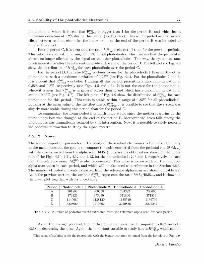
4.5. Stability of the photodiodes electronics 77
photodiode 4, where it is seen that RPedα/Ped is bigger than 1 for the period B, and which has a
maximum deviation of 1.2% during this period (see Fig. 4.7). This is interpreted as a cross-talkeffect between readout channels: the intervention at the end of the period B was intended toremove this effect.
For the period C, it is clear that the ratio RPedα/Ped is closer to 1 than for the previous periods.
This ratio is stable within a range of 0.3% for all photodiodes, which means that the pedestal isalmost no longer affected by the signal on the other photodiodes. This way, the system becamemuch more stable after the intervention made at the end of the period B. The left plots of Fig. 4.8show the distribution of RPed
α/Ped for each photodiode over the period C.For the period D, the ratio RPed
α/Ped is closer to one for the photodiode 1 than for the otherphotodiodes, with a maximum deviation of 0.25% (see Fig. 4.4). For the photodiodes 2 and 3,it is evident that RPed
α/Ped was below 1 during all this period, presenting a maximum deviation of0.35% and 0.3%, respectively (see Figs. 4.5 and 4.6). It is not the case for the photodiode 4,where it is seen that RPed
α/Ped is in general bigger than 1, and which has a maximum deviation ofaround 0.35% (see Fig. 4.7). The left plots of Fig. 4.9 show the distribution of RPed
α/Ped for each
photodiode for this period. This ratio is stable within a range of 0.35% for all photodiodes4.Looking at the mean value of the distributions of RPed
α/Ped, it is possible to see that the system wasslightly more stable during this period than for the period C.
To summarize, the mean pedestal is much more stable since the motherboard inside thephotodiodes box was changed at the end of the period B. Moreover the cross-talk among thephotodiodes was dramatically reduced by this intervention. Now, it is possible to safely performthe pedestal subtraction to study the alpha spectra.
4.5.1.2 Noise
The second important parameter in the study of the readout electronics is the noise. Similarlyto the mean pedestal, the goal is to compare the noise extracted from the pedestal run (RMSPed)with the one extracted from the alpha scan (RMSα). The results obtained are shown on the upperplot of the Figs. 4.10, 4.11, 4.12 and 4.13, for the photodiodes 1, 2, 3 and 4, respectively. In eachplot, the reference noise RefRMS
α is also represented. This noise is extracted from the referencealpha scan taken in each period, and which will be also used as a reference in the Section 4.6.3.The number of pedestal events extracted from the reference alpha scan are shown in Table 4.2.As in the previous section, the variable RRMS
α/Ped represents the ratio RMSα/RMSPed and is shown inthe lower plot together with its uncertainty.
Period Photodiode 1 Photodiode 2 Photodiode 3 Photodiode 4
A 201888 200658 204382 200666B 373426 373490 371800 371819C 1140680 1138120 1135510 1136760D 3228063 3219662 3210836 3225242
Table 4.2: Number of pedestal events extracted from the reference alpha scan for each period.
As for the average pedestal, the hardware interventions had an important effect on bothRMS by decreasing the noise. Again, the important variable to study here is RRMS
α/Ped, which should
4This range of stability is for the photodiode with the biggest variation obtained from the left plots in Fig. 4.9.
Daniela Paredes

78 Chapter 4. The TileCal Laser calibration system
11⁄04⁄02 11⁄07⁄02 11⁄10⁄01 12⁄01⁄01 12⁄04⁄01 12⁄07⁄01 12⁄10⁄01 12⁄12⁄31 13⁄04⁄01
RM
S
4.2
4.4
4.6
4.8
5
5.2αRMS
PedRMS
αRMSRef
ATLAS InternalTile Calorimeter
2011-13
Photodiode 1
date04/11 07/11 10/11 01/12 04/12 07/12 10/12 12/12 04/13
/Ped
αRM
SR
0.9
0.95
1
1.05
1.1
A B C D
Figure 4.10: Evolution of the noise measured in the pedestal run and the one extracted from the alphascan (top), and their ratio (bottom) for the photodiode 1 from February 2011 to February 2013. Theerror bars represent the statistical uncertainties on the averages and the ratios.
11⁄04⁄02 11⁄07⁄02 11⁄10⁄01 12⁄01⁄01 12⁄04⁄01 12⁄07⁄01 12⁄10⁄01 12⁄12⁄31 13⁄04⁄01
RM
S
4.5
5
5.5
6
6.5
αRMS
PedRMS
αRMSRef
ATLAS InternalTile Calorimeter
2011-13
Photodiode 2
date04/11 07/11 10/11 01/12 04/12 07/12 10/12 12/12 04/13
/Ped
αRM
SR
0.850.9
0.951
1.051.1
A B C D
Figure 4.11: Evolution of the noise measured in the pedestal run and the one extracted from the alphascan (top), and their ratio (bottom) for the photodiode 2 from February 2011 to February 2013. Theerror bars represent the statistical uncertainties on the averages and the ratios.
Daniela Paredes

4.5. Stability of the photodiodes electronics 79
11⁄04⁄02 11⁄07⁄02 11⁄10⁄01 12⁄01⁄01 12⁄04⁄01 12⁄07⁄01 12⁄10⁄01 12⁄12⁄31 13⁄04⁄01
RM
S
4.5
5
5.5
6
6.5 αRMS
PedRMS
αRMSRef
ATLAS InternalTile Calorimeter
2011-13
Photodiode 3
date04/11 07/11 10/11 01/12 04/12 07/12 10/12 12/12 04/13
/Ped
αRM
SR
0.9
0.95
1
1.05
1.1
A B C D
Figure 4.12: Evolution of the noise measured in the pedestal run and the one extracted from the alphascan (top), and their ratio (bottom) for the photodiode 3 from February 2011 to February 2013. Theerror bars represent the statistical uncertainties on the averages and the ratios.
11⁄04⁄02 11⁄07⁄02 11⁄10⁄01 12⁄01⁄01 12⁄04⁄01 12⁄07⁄01 12⁄10⁄01 12⁄12⁄31 13⁄04⁄01
RM
S
4
4.5
5
5.5
6
6.5
7
7.5
8 αRMS
PedRMS
αRMSRef
ATLAS InternalTile Calorimeter
2011-13
Photodiode 4
date04/11 07/11 10/11 01/12 04/12 07/12 10/12 12/12 04/13
/Ped
αRM
SR
0.95
1
1.05
1.1
1.15
1.2
A B C D
Figure 4.13: Evolution of the noise measured in the pedestal run and the one extracted from the alphascan (top), and their ratio (bottom) for the photodiode 4 from February 2011 to February 2013. Theerror bars represent the statistical uncertainties on the averages and the ratios.
Daniela Paredes

80 Chapter 4. The TileCal Laser calibration system
remain around 1: it would imply that the noise in the alpha scan is the same as the one in thepedestal run.
For the four periods, there are no significant changes in the ratio RRMSα/Ped for the photodi-
odes 2 and 3, which were rather stable with a maximum deviation of 7% for the periods A andB, and 6% for the period C (see Figs. 4.11 and 4.12). However, for the photodiodes 1 and 4,RRMSα/Ped has a range of 10% and 16% for the first two periods, and 4% and 5% for the period C,
respectively (see Figs. 4.10 and 4.13): the noise in these photodiodes has been well reduced inthe July, 2011 intervention and there is no longer a big discrepancy between the noise in thealpha scan and in the pedestal run. The plots on the center of Fig. 4.8 show the distribution ofRRMSα/Ped for each photodiode over the period C.
In general, for the periods A, B and C, the noise is a few percent higher in the alpha scanthan in the pedestal run, which may be related to the alpha source motor: during these threeperiods, it was powered on while the source was in front of the photodiodes. As a consequence,it could have introduced additional noise to the response of the electronics. As it was alreadyexplained, an intervention on December 5th, 2011 was done in order to solve this problem. Sincethen, the alpha source motor is powered off when it is in front of the photodiodes.
For the period D, no significant varioations are seen in the ratio RRMSα/Ped for all photodiodes,
which were rather stables with a maximum deviation of 4% for the photodiodes 2 and 4 (seeFigs. 4.11 and 4.13), and 5% for the photodiodes 1 and 3 (see Figs. 4.10 and 4.12). The plotson the center of Fig. 4.9 show the distribution of RRMS
α/Ped for each photodiode over this period.
This ratio is stable within a range of 4% for all photodiodes5. Looking at their mean values, itis possible to see that these ratios are closer to 1 for this period than for the period C. It meansthat the noise is under control for all photodiodes since the intervention done on December, 2011.
In particular, it is important to remark the good agreement between the noise extractedfrom both types of runs: the one extracted from the pedestal in the alpha scan and from thepedestal in the reference alpha scan for the periods C and D (see plots on the right side ofFigs. 4.8 and 4.9, respectively). A slightly better agreement between these runs is seen for theperiod D.
4.5.2 Linearity of the photodiodes electronics
Another crucial point for the understanding of the system is testing that the readout electronicsof the photodiodes used to measure the intensity of the laser light is linear.
The linearity of the photodiodes electronics is studied by injecting calibrated charges init. During the linearity runs, a Digital to Analog Converter (DAC) is used to set an electriclevel from which a charge proportional to the DAC level will be generated. Once this chargeis injected the response of the electronics is digitized by the ADC. Then, the response of thephotodiodes electronics and the value of the DAC level are recorded.
There are two ways of injecting charges in the photodiodes electronics: single and multi-charge injection modes. Both are explained below.
5As for the mean pedestal, this range of stability is for the photodiode with the biggest variation obtained fromthe center plots in Fig. 4.9.
Daniela Paredes

4.5. Stability of the photodiodes electronics 81
4.5.2.1 Single charge injection mode
This mode is used to make sure that the system that injects charges is stable. In this mode theinjected charge is constant. However, the measured value varies due to the noise introduced bythe electronics of the system. Thus, the response of the photodiodes electronics versus the chargeinjected to the four photodiodes looks like the plots shown in Fig. 4.14. The distribution of theinjected charge as well as the distribution of the response of the electronics of each photodiodeare shown in Fig. 4.15, together with a Gaussian fit. All the plots shown in both figures aremade after pedestal subtraction.
As can be seen from Fig. 4.15, the measured values of the injected charges are distributedfollowing a Gaussian distribution. The mean value of this distribution corresponds to the realinjected charge. As expected, the distribution of the response of the electronics of the photodiodesfollows the same distribution. This way we can conclude that the single charge injection systemis stable.
Injected charge1085 1090 1095 1100 1105 1110
Pho
todi
ode
resp
onse
1080
1090
1100
1110
1120
1130
1140Entries 999Mean x 1098Mean y 1112RMS x 1.537RMS y 3.985
0
5
10
15
20
25
30Entries 999Mean x 1098Mean y 1112RMS x 1.537RMS y 3.985
Photodiode 1
(a)
Injected charge1085 1090 1095 1100 1105 1110
Pho
todi
ode
resp
onse
1140
1150
1160
1170
1180
1190
1200
1210Entries 999Mean x 1098Mean y 1175RMS x 1.537RMS y 4.053
0
5
10
15
20
25
30
Entries 999Mean x 1098Mean y 1175RMS x 1.537RMS y 4.053
Photodiode 2
(b)
Injected charge1085 1090 1095 1100 1105 1110
Pho
todi
ode
resp
onse
1160
1170
1180
1190
1200
1210
1220 Entries 999Mean x 1098Mean y 1192RMS x 1.537RMS y 4.15
0
2
4
6
8
10
12
14
16
18
20
22Entries 999Mean x 1098Mean y 1192RMS x 1.537RMS y 4.15
Photodiode 3
(c)
Injected charge1085 1090 1095 1100 1105 1110
Pho
todi
ode
resp
onse
1130
1140
1150
1160
1170
1180
1190
1200Entries 999Mean x 1098Mean y 1166RMS x 1.537RMS y 4.196
0
5
10
15
20
25Entries 999Mean x 1098Mean y 1166RMS x 1.537RMS y 4.196
Photodiode 4
(d)
Figure 4.14: Response of the photodiodes electronics versus the injected charge for the photodiodes1 (a), 2 (b), 3 (c) and 4 (d), in the single charge injection mode after pedestal subtraction.
Daniela Paredes
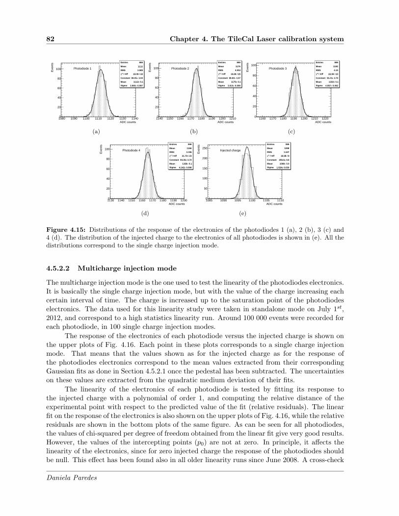
82 Chapter 4. The TileCal Laser calibration system
Entries 999
Mean 1112
RMS 3.985
/ ndf 2χ 18.09 / 22
Constant 3.94± 99.05
Mean 0.1± 1112
Sigma 0.097± 3.965
ADC counts1080 1090 1100 1110 1120 1130 1140
Eve
nts
0
20
40
60
80
100
Entries 999
Mean 1112
RMS 3.985
/ ndf 2χ 18.09 / 22
Constant 3.94± 99.05
Mean 0.1± 1112
Sigma 0.097± 3.965
Photodiode 1
(a)
Entries 999
Mean 1175
RMS 4.053
/ ndf 2χ 19.68 / 25
Constant 4.07± 99.84
Mean 0.1± 1175
Sigma 0.099± 3.915
ADC counts1140 1150 1160 1170 1180 1190 1200 1210
Eve
nts
0
20
40
60
80
100
Entries 999
Mean 1175
RMS 4.053
/ ndf 2χ 19.68 / 25
Constant 4.07± 99.84
Mean 0.1± 1175
Sigma 0.099± 3.915
Photodiode 2
(b)
Entries 999
Mean 1192
RMS 4.15
/ ndf 2χ 22.99 / 23
Constant 3.70± 95.41
Mean 0.1± 1192
Sigma 0.092± 4.097
ADC counts1160 1170 1180 1190 1200 1210 1220
Eve
nts
0
20
40
60
80
100Entries 999
Mean 1192
RMS 4.15
/ ndf 2χ 22.99 / 23
Constant 3.70± 95.41
Mean 0.1± 1192
Sigma 0.092± 4.097
Photodiode 3
(c)
Entries 999
Mean 1166
RMS 4.196
/ ndf 2χ 21.79 / 23
Constant 3.72± 94.35
Mean 0.1± 1166
Sigma 0.098± 4.142
ADC counts1130 1140 1150 1160 1170 1180 1190 1200
Eve
nts
0
20
40
60
80
100
Entries 999
Mean 1166
RMS 4.196
/ ndf 2χ 21.79 / 23
Constant 3.72± 94.35
Mean 0.1± 1166
Sigma 0.098± 4.142
Photodiode 4
(d)
Entries 999
Mean 1098
RMS 1.537
/ ndf 2χ 18.98 / 8
Constant 9.6± 256.6
Mean 0.0± 1098
Sigma 0.030± 1.524
ADC counts1085 1090 1095 1100 1105 1110
Eve
nts
0
50
100
150
200
250Entries 999
Mean 1098
RMS 1.537
/ ndf 2χ 18.98 / 8
Constant 9.6± 256.6
Mean 0.0± 1098
Sigma 0.030± 1.524
Injected charge
(e)
Figure 4.15: Distributions of the response of the electronics of the photodiodes 1 (a), 2 (b), 3 (c) and4 (d). The distribution of the injected charge to the electronics of all photodiodes is shown in (e). All thedistributions correspond to the single charge injection mode.
4.5.2.2 Multicharge injection mode
The multicharge injection mode is the one used to test the linearity of the photodiodes electronics.It is basically the single charge injection mode, but with the value of the charge increasing eachcertain interval of time. The charge is increased up to the saturation point of the photodiodeselectronics. The data used for this linearity study were taken in standalone mode on July 1st,2012, and correspond to a high statistics linearity run. Around 100 000 events were recorded foreach photodiode, in 100 single charge injection modes.
The response of the electronics of each photodiode versus the injected charge is shown onthe upper plots of Fig. 4.16. Each point in these plots corresponds to a single charge injectionmode. That means that the values shown as for the injected charge as for the response ofthe photodiodes electronics correspond to the mean values extracted from their correspondingGaussian fits as done in Section 4.5.2.1 once the pedestal has been subtracted. The uncertaintieson these values are extracted from the quadratic medium deviation of their fits.
The linearity of the electronics of each photodiode is tested by fitting its response tothe injected charge with a polynomial of order 1, and computing the relative distance of theexperimental point with respect to the predicted value of the fit (relative residuals). The linearfit on the response of the electronics is also shown on the upper plots of Fig. 4.16, while the relativeresiduals are shown in the bottom plots of the same figure. As can be seen for all photodiodes,the values of chi-squared per degree of freedom obtained from the linear fit give very good results.However, the values of the intercepting points (p0) are not at zero. In principle, it affects thelinearity of the electronics, since for zero injected charge the response of the photodiodes shouldbe null. This effect has been found also in all older linearity runs since June 2008. A cross-check
Daniela Paredes

4.5. Stability of the photodiodes electronics 83
0 200 400 600 800 1000 1200 1400 1600
Pho
todi
ode
resp
onse
0
500
1000
1500
2000
/ ndf 2χ 13.52 / 76p0 1.016± -31.64
p1 0.001019± 1.043
/ ndf 2χ 13.52 / 76p0 1.016± -31.64
p1 0.001019± 1.043
/ ndf 2χ 13.52 / 76p0 1.016± -31.64
p1 0.001019± 1.043
/ ndf 2χ 13.52 / 76p0 1.016± -31.64
p1 0.001019± 1.043
ATLAS InternalTile Calorimeter
2012-07-01
Photodiode 1
Injected charge0 200 400 600 800 1000 1200 1400 1600
Rel
. res
idua
ls
-0.04-0.02
00.020.040.060.08
0.1
(a)
0 200 400 600 800 1000 1200 1400 1600
Pho
todi
ode
resp
onse
0
500
1000
1500
2000
/ ndf 2χ 12.66 / 76p0 1.057± -47.57
p1 0.001064± 1.115
/ ndf 2χ 12.66 / 76p0 1.057± -47.57
p1 0.001064± 1.115
/ ndf 2χ 12.66 / 76p0 1.057± -47.57
p1 0.001064± 1.115
/ ndf 2χ 12.66 / 76p0 1.057± -47.57
p1 0.001064± 1.115
ATLAS InternalTile Calorimeter
2012-07-01
Photodiode 2
Injected charge0 200 400 600 800 1000 1200 1400 1600
Rel
. res
idua
ls
-0.04-0.02
00.020.040.060.08
0.1
(b)
0 200 400 600 800 1000 1200 1400 1600
Pho
todi
ode
resp
onse
0
500
1000
1500
2000
/ ndf 2χ 12.98 / 76p0 1.101± -48.97
p1 0.001103± 1.131
/ ndf 2χ 12.98 / 76p0 1.101± -48.97
p1 0.001103± 1.131
/ ndf 2χ 12.98 / 76p0 1.101± -48.97
p1 0.001103± 1.131
/ ndf 2χ 12.98 / 76p0 1.101± -48.97
p1 0.001103± 1.131
ATLAS InternalTile Calorimeter
2012-07-01
Photodiode 3
Injected charge0 200 400 600 800 1000 1200 1400 1600
Rel
. res
idua
ls
-0.04-0.02
00.020.040.060.08
0.1
(c)
0 200 400 600 800 1000 1200 1400 1600
Pho
todi
ode
resp
onse
0
500
1000
1500
2000
/ ndf 2χ 11.31 / 76p0 1.063± -47.67
p1 0.00107± 1.106
/ ndf 2χ 11.31 / 76p0 1.063± -47.67
p1 0.00107± 1.106
/ ndf 2χ 11.31 / 76p0 1.063± -47.67
p1 0.00107± 1.106
/ ndf 2χ 11.31 / 76p0 1.063± -47.67
p1 0.00107± 1.106
ATLAS InternalTile Calorimeter
2012-07-01
Photodiode 4
Injected charge0 200 400 600 800 1000 1200 1400 1600
Rel
. res
idua
ls
-0.04-0.02
00.020.040.060.08
0.1
(d)
Figure 4.16: Response of the photodiodes electronics versus the injected charge with the correspondingfitted line (top) for the photodiodes 1 (a), 2 (b), 3 (c) and 4 (d). The relative distance to the linear fit asa function of the injected charge is shown in the bottom plots.
was done by studying the linearity of the photodiodes electronics on a replica of the system, andthis effect is not present. The shift of the interception point can be attributed to variations inthe pedestal of the photodiodes or the injected charge. As the mean pedestal of the photodiodeselectronics measured in the linearity run coincide with the one measured in the pedestal run andin the alpha scan, that means that this difference can be assumed to come from a variation in thepedestal of the injected charge. This variation was estimated to be around 25%. Nevertheless,the effect of this kind of variations in the LASER calibration is considered to be negligible. As aconsequence, the linearity of the photodiodes here will be determined following only the goodnessof the linear fit, and the results of the relative residuals.
From the bottom plots in Fig. 4.16, it is possible to see that the relative residuals are within8% for all photodiodes, with statistical uncertainties that can raise to 20% when the injectedcharge is small, and which decrease as long as the injected charge increases. This behavior isexpected since the statistical uncertainty on the response of the photodiodes electronics is moreor less constant, independently of the numerical value of the response itself. Therefore, smallvalues of the response of photodiodes electronics will be affected in a greater proportion. Thedistributions of the relative residuals for each photodiode are shown in Fig. 4.17. As can be
Daniela Paredes

84 Chapter 4. The TileCal Laser calibration system
seen, most of the points are within 1% of the estimated fit.
Entries 68
Mean -0.0004627
RMS 0.001615
Rel. residuals-0.006 -0.004 -0.002 0 0.002 0.004 0.006
Ent
ries
0
2
4
6
8
10
12
14
Entries 68
Mean -0.0004627
RMS 0.001615Photodiode 1
(a)
Entries 68
Mean -0.0004265
RMS 0.001834
Rel. residuals-0.006 -0.004 -0.002 0 0.002 0.004 0.006
Ent
ries
0
2
4
6
8
10
12
14
16
Entries 68
Mean -0.0004265
RMS 0.001834Photodiode 2
(b)
Entries 68
Mean -0.0004627
RMS 0.00166
Rel. residuals-0.006 -0.004 -0.002 0 0.002 0.004 0.006
Ent
ries
0
2
4
6
8
10
12
14
16
Entries 68
Mean -0.0004627
RMS 0.00166Photodiode 3
(c)
Entries 68
Mean -0.0003529
RMS 0.001764
Rel. residuals-0.006 -0.004 -0.002 0 0.002 0.004 0.006
Ent
ries
0
2
4
6
8
10
12
14
16
18Entries 68
Mean -0.0003529
RMS 0.001764Photodiode 4
(d)
Figure 4.17: Distributions of the relative residuals for the photodiodes 1 (a), 2 (b), 3 (c) and 4 (d).Values at low injected charge have been excluded in these distributions.
A cross-check of these results can be done by using other linearity runs taken also instandalone mode on July, 2012. This is done by looking at the evolution of the slope (m) andthe interception point (p) given by the linear fit with respect to the reference values. These lastones correspond to the slope (p1) and the interception point (p0) obtained from the linear fitof the first linearity run taken on July, 2012 (this run also corresponds to the one analyzed inthis section, therefore the values of p0 and p1 are the ones shown in Fig. 4.16). The evolutionsof m/p1 and p/p0 are shown in Figs. 4.18(a) and 4.18(b), respectively. As can be seen, for thefour photodiodes the slope is stable within 0.2% with respect to the reference value, while theinterception point does within 4%.
4.5.3 Summary: stability of the photodiodes electronics
For all photodiodes the mean pedestal is much more stable after the intervention made at theend of the period B. Since then, the value measured in the alpha scans has had a maximumdeviation of 0.35% of the one measured in the pedestal runs. That means that the cross-talkwas dramatically reduced by this intervention. Now, the pedestal in the alpha scans is wellunderstood, i.e. it is possible to safely perform the pedestal subtraction to study the alphaspectra.
Daniela Paredes
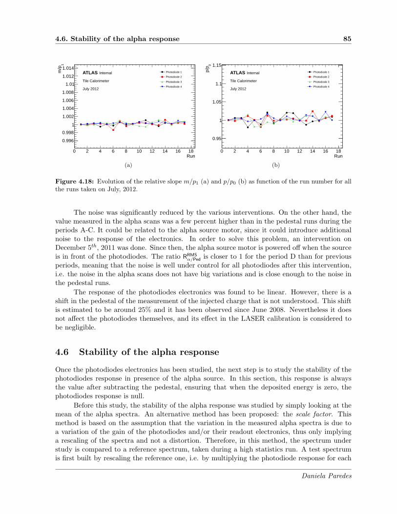
4.6. Stability of the alpha response 85
Run0 2 4 6 8 10 12 14 16 18
1m
/p
0.996
0.998
1
1.002
1.004
1.006
1.008
1.01
1.012
1.014Photodiode 1
Photodiode 2
Photodiode 3
Photodiode 4
ATLAS Internal
Tile Calorimeter
July 2012
(a)
Run0 2 4 6 8 10 12 14 16 18
0p/
p
0.95
1
1.05
1.1
1.15Photodiode 1
Photodiode 2
Photodiode 3
Photodiode 4
ATLAS Internal
Tile Calorimeter
July 2012
(b)
Figure 4.18: Evolution of the relative slope m/p1 (a) and p/p0 (b) as function of the run number for allthe runs taken on July, 2012.
The noise was significantly reduced by the various interventions. On the other hand, thevalue measured in the alpha scans was a few percent higher than in the pedestal runs during theperiods A-C. It could be related to the alpha source motor, since it could introduce additionalnoise to the response of the electronics. In order to solve this problem, an intervention onDecember 5th, 2011 was done. Since then, the alpha source motor is powered off when the sourceis in front of the photodiodes. The ratio RRMS
α/Ped is closer to 1 for the period D than for previousperiods, meaning that the noise is well under control for all photodiodes after this intervention,i.e. the noise in the alpha scans does not have big variations and is close enough to the noise inthe pedestal runs.
The response of the photodiodes electronics was found to be linear. However, there is ashift in the pedestal of the measurement of the injected charge that is not understood. This shiftis estimated to be around 25% and it has been observed since June 2008. Nevertheless it doesnot affect the photodiodes themselves, and its effect in the LASER calibration is considered tobe negligible.
4.6 Stability of the alpha response
Once the photodiodes electronics has been studied, the next step is to study the stability of thephotodiodes response in presence of the alpha source. In this section, this response is alwaysthe value after subtracting the pedestal, ensuring that when the deposited energy is zero, thephotodiodes response is null.
Before this study, the stability of the alpha response was studied by simply looking at themean of the alpha spectra. An alternative method has been proposed: the scale factor. Thismethod is based on the assumption that the variation in the measured alpha spectra is due toa variation of the gain of the photodiodes and/or their readout electronics, thus only implyinga rescaling of the spectra and not a distortion. Therefore, in this method, the spectrum understudy is compared to a reference spectrum, taken during a high statistics run. A test spectrumis first built by rescaling the reference one, i.e. by multiplying the photodiode response for each
Daniela Paredes

86 Chapter 4. The TileCal Laser calibration system
recorded event by a constant number, called the scale factor. Then, this scale factor is varieduntil the resulting distribution fits as well as possible the one under study. The resulting scalefactor is then a measurement of the gain variation, being equal to one if no rescaling is neededto fit the reference distribution to the studied one.
In Section 4.6.1, the two methods, scale factor and normalized mean value, are comparedusing simulated data. It will be demonstrated that the scale factor is more sensitive than themean value. Then, in Section 4.6.2, it will be studied, still on simulated data, the bias introducedon the scale factor determination by uncontrolled variations of the pedestal and the noise. Theseeffects will also be studied on the mean value method. Finally, in Section 4.6.3, the scale factormethod will be applied on all alpha scans taken between 2011 and 2013 in order to study thestabillty of the photodiodes over this period.
4.6.1 Comparison of the scale factor and mean value methods
In this section, the two criteria to study the stability of the alpha response will be compared:mean value and scale factor. In order to evaluate the relative precision and stability of the twoapproaches, pseudoexperiments are generated, and are explained in the following paragraph.
A simulated alpha scan is generated in order to simulate the impact of a constant scaleshift. The first step consists in generating a distribution with the same shape as the referencedata (Fig. 4.19(a)), but with a lower statistics (the same statistics as the data taken during thestop of the ATLAS run, i.e. 10000 events). The reference data corresponds to the first LongLaser Alpha Scan taken in 2012 (1074848 events) for the photodiode 2. The lower statisticsreference (see Fig. 4.19(b)) is then multiplied by a scale factor SF0 , the resulting distribution isthe simulated alpha scan (Fig. 4.19(c)).
Entries 1074848
Mean 814.5
RMS 82.8
ADC counts300 400 500 600 700 800 900 1000 1100
Eve
nts
0
5000
10000
15000
20000
25000
30000
35000
Entries 1074848
Mean 814.5
RMS 82.8
(a) Reference data
⇒
Entries 10000
Mean 814.2
RMS 83.07
ADC counts300 400 500 600 700 800 900 1000 1100
Eve
nts
0
50
100
150
200
250
300
350Entries 10000
Mean 814.2
RMS 83.07
(b) Reference data with a lowstatistics
⇒
Entries 10000
Mean 651.4
RMS 66.45
ADC counts400 500 600 700 800
Eve
nts
0
50
100
150
200
250
300
350
400
Entries 10000
Mean 651.4
RMS 66.45
(c) Simulated alpha scan
Figure 4.19: From the reference data is generated a distribution with a low statistics, which is thenmultiplied by the scale factor SF0 in order to obtain the simulated alpha scan. In this example SF0 = 0.8.
The procedure in order to compare the methods can be described as:
Scale factor:
1. The reference spectrum is multiplied by a scale factor SF1. Then the values of χ2/ndf andthe p-value between this distribution and the simulated alpha scan are computed using theχ2 and Kolmogorov tests, respectively.
2. The previous step is repeated for different values of SF1. The goal is to construct a plotof χ2/ndf as a function of SF1, and the p-value also as a function of SF1: the scale factor
Daniela Paredes

4.6. Stability of the alpha response 87
with the minimum (maximum) value of χ2 (p-value), i.e. the simulated alpha scan thatbetter fits the reference data, is the best scale factor found for this simulated alpha scan(see plots in Fig. 4.20).
1SF0.99 0.995 1 1.005 1.01
/ndf
2 χ
0
5
10
15
20
25
30
1SF0.99 0.995 1 1.005 1.01
p-va
lue
0
0.2
0.4
0.6
0.8
1
Figure 4.20: Example of a plot of χ2/ndf (left) and p-value (right) as a function of the scale factor SF1
for a simulated alpha scan. Both plots correspond to a scale factor SF0 = 1. The best scale factor foundin both cases corresponds to SF1 = 1.0001.
3. A new simulated alpha scan is generated and the two previous steps are repeated (usingthe same value for SF0) to obtain a distribution SF1/SF0. This distribution is shown inFig. 4.21(a) for the χ2 test, and Fig. 4.21(b) for the Kolmogorov test. The width of thesedistributions gives the precision of the method. The value of χ2/ndf (p-value) as a functionof the best scale factor found SF1 for each simulated alpha scan generated is shown in theright (left) plot of Fig. 4.22.
Mean value:
1. The mean value of the reference data, µ0, is computed.
2. The mean value of the simulated alpha scan, µ1, is computed.
3. A new simulated alpha scan is generated and the previous step is repeated to obtain adistribution µ1/(µ0 × SF0) (see Fig. 4.21(c)) for the same value of SF0. Again, the widthof the distribution gives the precision of the method.
From the results in Figs. 4.21(a)-4.21(c), it is possible to see that the three distributionsare well centered on 1. As can be seen from Figs. 4.21(a) and 4.21(b), the standard deviations ofthe distributions SF1/SF0 are σSF = 0.00028 and σSF = 0.00052, respectively. They are smallerthan the one extracted from the distribution µ1/(µ0×SF0), σµ = 0.0010 (see Fig. 4.21(c)). Thissituation is more visible in Fig. 4.21(d). It means that the scale factor is a more precise methodthan the mean value.
All plots presented in this section correspond to a scale factor SF0 = 1, and for an alphaspectrum with 500 bins. In principle, in the scale factor method, χ2 gives better results thanthe Kolomogorov test, since the standard deviation of its distribution SF1/SF0 is smaller. Nev-ertheless, it is necessary to check if these results are stable when different values of SF0 are used.
Daniela Paredes

88 Chapter 4. The TileCal Laser calibration system
Entries 50000
Mean 1
RMS 0.0002842
0/SF1SF0.996 0.998 1 1.002 1.004
Ent
ries
0
1000
2000
3000
4000
5000
6000
7000
8000
Entries 50000
Mean 1
RMS 0.0002842
(a)
Entries 50000
Mean 1
RMS 0.0005218
0/SF1SF0.996 0.998 1 1.002 1.004
Ent
ries
0
500
1000
1500
2000
2500
3000
3500
Entries 50000
Mean 1
RMS 0.0005218
(b)
Entries 50000
Mean 1
RMS 0.001014
)0 SF×0
µ/(1
µ0.996 0.998 1 1.002 1.004
Ent
ries
0
200
400
600
800
1000
1200
1400
1600
1800
2000Entries 50000
Mean 1
RMS 0.001014
(c)
Entries 50000
Mean 1
RMS 0.0002842
0/SF1SF0.996 0.998 1 1.002 1.004
Ent
ries
0
1000
2000
3000
4000
5000
6000
7000
8000Entries 50000
Mean 1
RMS 0.0002842
Entries 50000
Mean 1
RMS 0.0005218
Entries 50000
Mean 1
RMS 0.001013
test)2χ (0/SF1SF
(Kolmogorov test)0
/SF1
SF
)0 SF×0
µ/(1
µ
(d)
Figure 4.21: Distributions of SF1/SF0 obtained using the χ2 test (a) and the Kolmogorov test (b). Thedistribution of µ1/(µ0×SF0) is shown in (c). The comparison of these three distributions is shown in (d).In this example 50 000 pseudoexperiments were generated and SF0 = 1.
1SF0.997 0.998 0.999 1 1.001 1.002 1.003
/ndf
2 χ
0.2
0.4
0.6
0.8
1
1.2
1.4
1.6
1.8
2
2.2Entries 50000Mean x 1Mean y 0.9735RMS x 0.0002842RMS y 0.1142
Entries 50000Mean x 1Mean y 0.9735RMS x 0.0002842RMS y 0.1142
1SF0.994 0.996 0.998 1 1.002 1.004 1.006
p-va
lue
0
0.1
0.2
0.3
0.4
0.5
0.6
0.7
0.8
0.9
1Entries 50000Mean x 1Mean y 0.8228RMS x 0.0005218RMS y 0.1996
Entries 50000Mean x 1Mean y 0.8228RMS x 0.0005218RMS y 0.1996
Figure 4.22: χ2/ndf (left) and p-value (right) as a function of the best scale factor found SF1 for eachsimulated alpha scan. These values have been computed using the χ2 test and the Kolmogorov test,respectively. In this example SF0 = 1.
Daniela Paredes

4.6. Stability of the alpha response 89
The values tested here go from SF0 = 0.8 to SF0 = 1.2 per steps of 0.002. The distributions of〈SF1/SF0〉 obtained using both methods, χ2 and the Kolmogorov tests are shown in Fig. 4.23(a).The distribution of 〈µ1/(µ0×SF0)〉 is also shown in this plot. As can be seen, the results obtainedfrom the Kolmogorov test are well centered in 1, while the scale factors computed using the χ2
test are biased to values bigger than SF0. This bias becomes more important when the binning ofthe alpha spectra decreases (see Figs. 4.23(b) and 4.23(c)), with a maximum deviation of 0.51%.Scale factors computed via the Kolmogorov test are stable within 0.005%. For that reason, theKolmogorov test will be used to determine the stability of the alpha spectra with the scale factormethod.
The standard deviations extracted from the distributions SF1/SF0 and µ1/(µ0 × SF0) fora range between SF0 = 0.8 and SF0 = 1.2 per steps of 0.002 are shown in Fig. 4.24. As can beseen the standard deviation for the scale factor is always smaller than the one for the normalizedmean value. It corroborates that the scale factor is a more precise method than the mean value.Therefore, it will be the main method used to monitor the stability of the alpha spectra via theKolmogorov test.
Entries 200Mean 1RMS 1.927e-05
0.9999 1 1.00011.00021.00031.00041.00051.0006
Ent
ries
0
20
40
60
80
100
120
140
160
180
200
Entries 200Mean 1RMS 1.927e-05
test2χ: ⟩0/SF1
SF⟨
: Kolmogorov test⟩0/SF1
SF⟨
⟩)0 SF×0
µ/(1
µ⟨
(a)
Entries 201
Mean 1
RMS 2.188e-05
0.9999 1 1.00011.00021.00031.00041.00051.0006
Ent
ries
0
20
40
60
80
100
120
140
160
180
200
Entries 201
Mean 1
RMS 2.188e-05
test2χ: ⟩0/SF1
SF⟨
: Kolmogorov test⟩0/SF1
SF⟨
⟩)0 SF×0
µ/(1
µ⟨
(b)
Entries 201
Mean 1
RMS 0.000129
0.9999 1 1.00011.00021.00031.00041.00051.0006
Ent
ries
0
20
40
60
80
100
120
140
160
180
200
Entries 201
Mean 1
RMS 0.000129
test2χ: ⟩0/SF1
SF⟨
: Kolmogorov test⟩0/SF1
SF⟨
⟩)0 SF×0
µ/(1
µ⟨
(c)
Figure 4.23: Distributions of 〈SF1/SF0〉 obtained using both methods, χ2 and the Kolmogorov test foralpha spectra with 750 (a), 500 (b) and 250 (c) bins. The distribution of 〈µ1/(µ0 × SF0)〉 is also shown ineach plot. The values of SF0 used go from 0.8 to 1.2 per steps of 0.002.
Daniela Paredes

90 Chapter 4. The TileCal Laser calibration system
0SF0.8 0.85 0.9 0.95 1 1.05 1.1 1.15 1.2
σ
0
0.0002
0.0004
0.0006
0.0008
0.001
0.0012
0.0014⟩0/SF
1 SF⟨
⟩)0 SF×0
µ/(1
µ⟨
Figure 4.24: Standard deviation of µ1/(µ0 × SF0) (black) and SF1/SF0 (red) for SF0 = 0.8 to SF0 = 1.2per steps of 0.002.
4.6.2 Effects on the scale factor and mean value of variations in the readoutelectronics
As stated previously, the scale factor method assumes that there is no distortion of the alphaspectra, only rescaling. Distortion could arise from variations of the characteristics of the readoutelectronics, pedestal and noise. Therefore, in this section, it will study, still using pseudoexper-iments, the effect of adding variations of the readout electronics characteristics on the alpharesponse, using the Kolmogorov test to determine the scale factor. The procedure in order toproduce these simulated data is equivalent to the one presented in the previous section: from areference data is generated a distribution with a low statistics, but here a constant variation ofthe readout electronics is added, the resulting distribution is the simulated alpha scan.
In order to determine the scale factor and mean value, the same procedure presented inthe Section 4.6.1 is used. This time, the interest resides in obtaining the distributions ∆µ(%) =[µ1/(µ0 × SF0)− 1]× 100 and ∆SF(%) = (SF1/SF0 − 1)× 100 for the mean value and the scalefactor, respectively. The mean value of these distributions gives the variation in the scale factoror mean value for the specific variation of the readout electronics. The goal is to construct a plotof ∆SF(%) and ∆µ(%) as a function of this variation.
The studied variations of the readout electronics are the pedestal and noise variations. Theeffect of each one of them is studied separately.
An example of the distributions ∆SF(%) and ∆µ(%) for a scale factor SF0 = 1 and apedestal variation ∆p = 1% is shown in the Fig. 4.25. From there, it is possible to see that thescale factor is shifted by 0.21% if a pedestal variation of 1% is added. A similar result is obtainedfor the mean value: 0.22%.
The plots of the ∆SF(%) and ∆µ(%) for different values of SF0 as a function of the pedestalvariation can be found in the left and right sides of the Fig. 4.26, respectively. The error barsrepresent the standard deviation of the distributions ∆SF(%) or ∆µ(%) for the given pedestalvariation. The range of the pedestal variation studied goes from -10% to +10%. As can be seen,in both cases the relation is linear, the slope of each line gives the sensitivity of its respectivemethod with respect to the parameter studied. For SF0 = 1, the scale factor has a sensitivityof ≈ 0.21%, while for the mean value it is ≈ 0.22%, but its uncertainty is bigger than for thescale factor. Basically, the two methods have almost the same sensitivity, which means the same
Daniela Paredes

4.6. Stability of the alpha response 91
bias. In a few words, if the knowledge of the pedestal in the real data is bad, it will result in thesame bias for the scale factor as for the mean value. It is important to remark that for a givenvariation of the pedestal, the bias depends very weakly on SF0.
Entries 50000Mean 0.2142RMS 0.05222
-0.2 -0.1 0 0.1 0.2 0.3 0.4 0.5 0.6
Ent
ries
0
500
1000
1500
2000
2500
3000
3500Entries 50000Mean 0.2142RMS 0.05222
Entries 50000
Mean 0.2249
RMS 0.1013
SF(%)∆(%)µ∆
Figure 4.25: An example of the distributions ∆SF(%) and ∆µ(%) for a pedestal variation ∆p = 1%.
p(%)∆-10 -5 0 5 10
SF
(%)
∆
-2
-1
0
1
2=0.90SF
=10SF=1.10SF
p(%)∆-10 -5 0 5 10
(%)
µ∆
-2
-1
0
1
2 =0.90SF
=10SF=1.10SF
Figure 4.26: Variation of the scale factor (left side) and of the mean value (right side) as a function ofthe pedestal variation ∆p.
From the real data, the estimation of the pedestal in the alpha scan may be wrong by atmost 0.35% for the period D (see left plots of Fig. 4.9), such error would imply a shift in thescale factor (or mean value) of ≈ 0.07%, a small value but detectable.
About the noise, an example of the distributions ∆SF(%) and ∆µ(%) for a scale factorSF0 = 1 and a noise variation ∆σ = 50% is shown in the left side of the Fig. 4.27. The rangestudied goes from -100% to +100%. Again, the error bars represent the standard deviation ofthe distributions ∆SF(%) or ∆µ(%) for the given noise variation. As can be seen, the variationin the scale factor is very small: it just changes in only ≈0.0006% when 50% of noise is added.The plot of the ∆SF(%) for different values of SF0 as a function of the noise variation is shownin the right plot of the same figure. In contrast to the pedestal variation, the relation here isnot linear. Again, a variation of 10% in SF0 for noise variations between -50% and +50% would
Daniela Paredes

92 Chapter 4. The TileCal Laser calibration system
leave the shift in the scale factor practically unchanged. The effect on the mean value within therange is less than 0.001%, which is undetectable at this level.
Entries 50000
Mean 0.0005834
RMS 0.05215
0/SF1SF-0.4 -0.2 0 0.2 0.4
Ent
ries
0
500
1000
1500
2000
2500
3000
3500Entries 50000
Mean 0.0005834
RMS 0.05215
Entries 50000
Mean 0.0007926
RMS 0.1021
SF(%)∆(%)µ∆
(%)σ∆-100 -50 0 50 100
SF
(%)
∆
-0.06
-0.04
-0.02
0
0.02
0.04
0.06
0.08
0.1
0.12
=0.90SF
=10SF=1.10SF
Figure 4.27: Left: an example of the distributions ∆SF(%) and ∆µ(%) for a noise variation ∆σ = 50%.Right: variation of the scale factor as a function of the noise variation.
In the real data, noise variations are smaller than 5% for the period D (see middle plotsin Fig. 4.9), which corresponds to a shift in the scale factor of ≈0.0003%, which is completelynegligible.
From this study, it is possible to conclude that an approximative knowledge of the pedestalwithin the range established in Section 4.5.1.1 would have a small but detectable effect on boththe scale factor and the mean value. The variations of the noise observed in Section 4.5.1.2 arecompletely negligible.
4.6.3 Stability of the alpha response from 2011 to 2013
As determined in Section 4.6.1 the scale factor will be the main method to monitor the stabilityof the alpha spectra. The procedure applied for each alpha scan is described as follows:
1. The reference data is multiplied by a scale factor SF1. Then, the probability of equalitybetween this distribution and the alpha spectrum extracted from the alpha scan is com-puted using the Kolmogorov test. The number of recorded events of the reference data isgiven in the Table 4.3.
Period Photodiode 1 Photodiode 2 Photodiode 3 Photodiode 4
A 67305 68537 64811 68523B 123409 123348 125025 125018C 376322 378869 381486 380250D 1066460 1074850 1083680 1069270
Table 4.3: Number of recorded events of the reference data used for each period for each photodiode.
Daniela Paredes
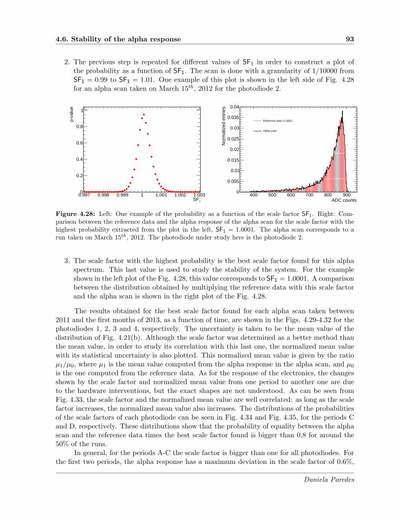
4.6. Stability of the alpha response 93
2. The previous step is repeated for different values of SF1 in order to construct a plot ofthe probability as a function of SF1. The scan is done with a granularity of 1/10000 fromSF1 = 0.99 to SF1 = 1.01. One example of this plot is shown in the left side of Fig. 4.28for an alpha scan taken on March 15th, 2012 for the photodiode 2.
1SF0.997 0.998 0.999 1 1.001 1.002 1.003
p-va
lue
0
0.2
0.4
0.6
0.8
1
Entries 999895Mean 814.7RMS 82.77
ADC counts400 500 600 700 800 900
Nor
mal
ized
ent
ries
0
0.005
0.01
0.015
0.02
0.025
0.03
0.035
0.04
Entries 999895Mean 814.7RMS 82.77
1.0001×Reference data
Alpha scan
Figure 4.28: Left: One example of the probability as a function of the scale factor SF1. Right: Com-parison between the reference data and the alpha response of the alpha scan for the scale factor with thehighest probability extracted from the plot in the left, SF1 = 1.0001. The alpha scan corresponds to arun taken on March 15th, 2012. The photodiode under study here is the photodiode 2.
3. The scale factor with the highest probability is the best scale factor found for this alphaspectrum. This last value is used to study the stability of the system. For the exampleshown in the left plot of the Fig. 4.28, this value corresponds to SF1 = 1.0001. A comparisonbetween the distribution obtained by multiplying the reference data with this scale factorand the alpha scan is shown in the right plot of the Fig. 4.28.
The results obtained for the best scale factor found for each alpha scan taken between2011 and the first months of 2013, as a function of time, are shown in the Figs. 4.29-4.32 for thephotodiodes 1, 2, 3 and 4, respectively. The uncertainty is taken to be the mean value of thedistribution of Fig. 4.21(b). Although the scale factor was determined as a better method thanthe mean value, in order to study its correlation with this last one, the normalized mean valuewith its statistical uncertainty is also plotted. This normalized mean value is given by the ratioµ1/µ0, where µ1 is the mean value computed from the alpha response in the alpha scan, and µ0is the one computed from the reference data. As for the response of the electronics, the changesshown by the scale factor and normalized mean value from one period to another one are dueto the hardware interventions, but the exact shapes are not understood. As can be seen fromFig. 4.33, the scale factor and the normalized mean value are well correlated: as long as the scalefactor increases, the normalized mean value also increases. The distributions of the probabilitiesof the scale factors of each photodiode can be seen in Fig. 4.34 and Fig. 4.35, for the periods Cand D, respectively. These distributions show that the probability of equality between the alphascan and the reference data times the best scale factor found is bigger than 0.8 for around the50% of the runs.
In general, for the periods A-C the scale factor is bigger than one for all photodiodes. Forthe first two periods, the alpha response has a maximum deviation in the scale factor of 0.6%,
Daniela Paredes

94 Chapter 4. The TileCal Laser calibration system
date04/11 07/11 10/11 01/12 04/12 07/12 10/12 12/12 04/13
0.99
0.995
1
1.005
1.01
1.015
A B C D
Scale Factor
Normalized mean value
ATLAS Internal
Tile Calorimeter
2011-13 Photodiode 1
Figure 4.29: Evolution of the scale factor and the normalized mean value for the photodiodes 1 between2011 and the first months of 2013.
date04/11 07/11 10/11 01/12 04/12 07/12 10/12 12/12 04/13
0.99
0.995
1
1.005
1.01
1.015
A B C D
Scale Factor
Normalized mean value
ATLAS Internal
Tile Calorimeter
2011-13 Photodiode 2
Figure 4.30: Evolution of the scale factor and the normalized mean value for the photodiodes 2 between2011 and the first months of 2013.
Daniela Paredes
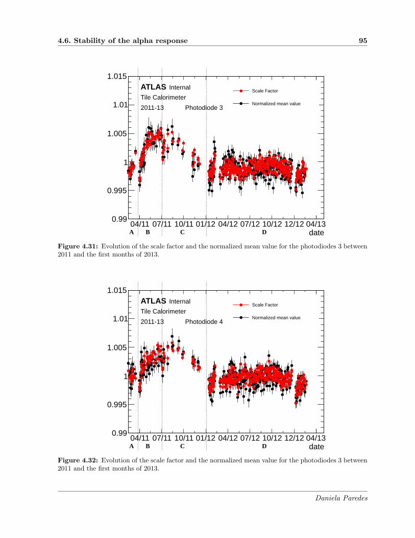
4.6. Stability of the alpha response 95
date04/11 07/11 10/11 01/12 04/12 07/12 10/12 12/12 04/13
0.99
0.995
1
1.005
1.01
1.015
A B C D
Scale Factor
Normalized mean value
ATLAS Internal
Tile Calorimeter
2011-13 Photodiode 3
Figure 4.31: Evolution of the scale factor and the normalized mean value for the photodiodes 3 between2011 and the first months of 2013.
date04/11 07/11 10/11 01/12 04/12 07/12 10/12 12/12 04/13
0.99
0.995
1
1.005
1.01
1.015
A B C D
Scale Factor
Normalized mean value
ATLAS Internal
Tile Calorimeter
2011-13 Photodiode 4
Figure 4.32: Evolution of the scale factor and the normalized mean value for the photodiodes 3 between2011 and the first months of 2013.
Daniela Paredes

96 Chapter 4. The TileCal Laser calibration system
Scale factor0.992 0.994 0.996 0.998 1 1.002 1.004
Nor
mal
ized
mea
n va
lue
0.992
0.994
0.996
0.998
1
1.002
1.004
Entries 0Mean x 0Mean y 0RMS x 0RMS y 0
Entries 0Mean x 0Mean y 0RMS x 0RMS y 0
Photodiode 1
(a)
Scale factor0.992 0.994 0.996 0.998 1 1.002 1.004
Nor
mal
ized
mea
n va
lue
0.992
0.994
0.996
0.998
1
1.002
1.004
Entries 0Mean x 0Mean y 0RMS x 0RMS y 0
Entries 0Mean x 0Mean y 0RMS x 0RMS y 0
Photodiode 2
(b)
Scale factor0.992 0.994 0.996 0.998 1 1.002 1.004
Nor
mal
ized
mea
n va
lue
0.992
0.994
0.996
0.998
1
1.002
1.004
Entries 0Mean x 0Mean y 0RMS x 0RMS y 0
Entries 0Mean x 0Mean y 0RMS x 0RMS y 0
Photodiode 3
(c)
Scale factor0.992 0.994 0.996 0.998 1 1.002 1.004
Nor
mal
ized
mea
n va
lue
0.992
0.994
0.996
0.998
1
1.002
1.004
Entries 0Mean x 0Mean y 0RMS x 0RMS y 0
Entries 0Mean x 0Mean y 0RMS x 0RMS y 0
Photodiode 4
(d)
Figure 4.33: Normalized mean value as a function of the scale factor found of the photodiodes 1 (a),2 (b), 3 (c) and 4 (d) for all the alpha scans taken in the period D.
p-value0 0.2 0.4 0.6 0.8 1
Ent
ries
0
1
2
3
4
5
6
7Photodiode 1
(a)
p-value0 0.2 0.4 0.6 0.8 1
Ent
ries
0
1
2
3
4
5
6Photodiode 2
(b)
p-value0 0.2 0.4 0.6 0.8 1
Ent
ries
0
1
2
3
4
5
6
7Photodiode 3
(c)
p-value0 0.2 0.4 0.6 0.8 1
Ent
ries
0
1
2
3
4
5
6
7Photodiode 4
(d)
Figure 4.34: Distributions of the probabilities of the scale factors found of the photodiodes 1 (a), 2 (b),3 (c) and 4 (d) for all the alpha scans taken in the period C.
Daniela Paredes

4.6. Stability of the alpha response 97
p-value0 0.2 0.4 0.6 0.8 1
Ent
ries
10
20
30
40
50
60
70 Photodiode 1
(a)
p-value0 0.2 0.4 0.6 0.8 1
Ent
ries
10
20
30
40
50
60Photodiode 2
(b)
p-value0 0.2 0.4 0.6 0.8 1
Ent
ries
10
20
30
40
50
60Photodiode 3
(c)
p-value0 0.2 0.4 0.6 0.8 1
Ent
ries
10
20
30
40
50
60
70Photodiode 4
(d)
Figure 4.35: Distributions of the probabilities of the scale factors found of the photodiodes 1 (a), 2 (b),3 (c) and 4 (d) for all the alpha scans taken in the period D.
0.7%, 0.6% and 0.6%, for the photodiodes 1, 2, 3 and 4, respectively (see Figs. 4.29-4.32). A littleimprovement is seen in the period C for the photodiode 2, where the scale factor is closer to 1 thanfor the previous periods, with a maximum deviation of 0.5%. However, for the photodiodes 1, 3and 4, although their stability was within a range of 0.6%, the hardware interventions do notseem to have improved them. The distributions of the scale factors for each photodiode can beseen in Fig. 4.36 for the period C.
In contrast with the periods A-C, the scale factor is slightly smaller than one for allphotodiodes (see Fig. 4.37) for the period D. No significant variations were observed in thealpha response during this period, where the scale factor was rather stable with a maximumdeviation of 0.4% for the photodiode 1, and 0.5% for the remaining photodiodes (see Figs. 4.29-4.32). It represents a slight improvement with respect to the period C.
As stated in Section 4.6.2, pedestal variations can introduce small variations in both thescale factor and the mean normalized value, with the same bias for both methods. From the realdata, the estimation of the pedestal in the alpha scan may be wrong by at most 0.35%. Sucherror would imply a shift in the scale factor or normalized mean value of ≈ 0.07%, a small valuebut detectable, and which can explain around 14% of the variation in the scale factor for thedata taken in the period D. Uncontrolled noise variations of around 5% were found in the data,and as it was shown in Section 4.6.2, variations of this order do not affect the scale factor.
Daniela Paredes

98 Chapter 4. The TileCal Laser calibration system
Entries 23
Mean 1.003
RMS 0.001299
Scale Factor0.996 0.998 1 1.002 1.004 1.006 1.008
Ent
ries
0
1
2
3
4
5
6
7Entries 23
Mean 1.003
RMS 0.001299
Photodiode 1
(a)
Entries 23
Mean 1.002
RMS 0.0009404
Scale Factor0.996 0.998 1 1.002 1.004 1.006 1.008
Ent
ries
0
1
2
3
4
5
6
7
8
9Entries 23
Mean 1.002
RMS 0.0009404
Photodiode 2
(b)
Entries 23
Mean 1.002
RMS 0.001621
Scale Factor0.996 0.998 1 1.002 1.004 1.006 1.008
Ent
ries
0
1
2
3
4
5
6Entries 23
Mean 1.002
RMS 0.001621Photodiode 3
(c)
Entries 23
Mean 1.003
RMS 0.001343
Scale Factor0.996 0.998 1 1.002 1.004 1.006 1.008
Ent
ries
0
1
2
3
4
5
6Entries 23
Mean 1.003
RMS 0.001343
Photodiode 4
(d)
Figure 4.36: Distributions of the scale factors of the photodiodes 1 (a), 2 (b), 3 (c) and 4 (d) for all thealpha scans in the period C.
Entries 314
Mean 0.9987
RMS 0.0007597
Scale Factor0.996 0.998 1 1.002 1.004
Ent
ries
0
20
40
60
80
100
120
140
160Entries 314
Mean 0.9987
RMS 0.0007597
Photodiode 1
(a)
Entries 314
Mean 0.9994
RMS 0.0008959
Scale Factor0.996 0.998 1 1.002 1.004
Ent
ries
0
20
40
60
80
100
120
Entries 314
Mean 0.9994
RMS 0.0008959
Photodiode 2
(b)
Entries 314
Mean 0.9989
RMS 0.001069
Scale Factor0.996 0.998 1 1.002 1.004
Ent
ries
0
20
40
60
80
100
Entries 314
Mean 0.9989
RMS 0.001069
Photodiode 3
(c)
Entries 314
Mean 0.9995
RMS 0.001123
Scale Factor0.996 0.998 1 1.002 1.004
Ent
ries
0
20
40
60
80
100
Entries 314
Mean 0.9995
RMS 0.001123
Photodiode 4
(d)
Figure 4.37: Distributions of the scale factors of the photodiodes 1 (a), 2 (b), 3 (c) and 4 (d) for all thealpha scans in the period D.
Daniela Paredes

4.7. Summary and conclusions 99
4.6.4 Summary: stability of the alpha response
It was demonstrated that the scale factor –via the Kolmogorov test– is a more sensitive methodthan the mean value in order to study the stability of the alpha response, which was stable witha maximum deviation of 0.5% for all the data taken in 2012 and the first months of 2013. Itrepresents a slight improvement with respect to the year 2011.
It was also found that an uncontrolled pedestal variation for this period explains only avery small part of the variation in the scale factor. The noise variation is completely negligible.
Finally, it was observed that the scale factor and the normalized mean value are wellcorrelated for all photodiodes.
4.7 Summary and conclusions
A precise knowledge of the photodiodes response is the first step towards the understandingof the LASER system. In order to monitor the stability of the photodiodes it is essential tounderstand their readout electronics, as well as the stability of the alpha response.
The stability of the photodiodes was monitored using data taken between 2011 and thefirst months of 2013. This monitoring activity has been split in four different periods, wheretwo periods are separated by a hardware intervention. For all photodiodes, the mean pedestal ismuch more stable after the intervention made at the end of the period B. That means that thepedestal of each photodiode is no longer affected by the signal on the other ones: the cross-talkamong the photodiodes has been dramatically reduced by the July, 2011 hardware intervention.Now, the pedestal in the alpha scan is well understood, i.e. it is possible to safely perform thepedestal subtraction to study the alpha spectra.
The noise was significantly reduced by the various interventions. On the other hand, thevalue measured in the alpha scans was a few percent higher than in the pedestal runs during theperiods A-C. It could be related to the alpha source motor, since it could introduce additionalnoise to the response of the electronics. In order to solve this problem, an intervention onDecember 5th, 2011 was done. Since then, the alpha source motor is powered off when thesource is in front of the photodiodes. Now the noise extracted from the pedestal in the alphascans is closer to the one extracted from the pedestal runs, meaning that the noise is undercontrol for all photodiodes after this intervention.
The response of the photodiodes electronics was also found to be linear. However, there isa shift in the injected charge pedestal that is not understood. This shift is estimated to be around25% and it has been observed since June 2008. Nevertheless it does not affect the photodiodesthemselves, and its effect in the LASER calibration is negligible.
It was demonstrated that the scale factor is a more precise method than the mean value.From the beginning of 2012, the worst observed variation in the photodiode gain was 0.5%which is within the acceptable variations for the photodiodes system. Following the studies doneabout the effects on the scale factor and mean value of variations in the readout electronicscharacteristics, it was found that pedestal or noise variations are not sufficient to explain thevariations found in the scale factor.
As a general conclusion, the change of the motherboard inside the photodiodes box hada big effect in the system by making it much more stable. Moreover, the photodiodes absoluteresponse is stable within a range of 0.5%. This value could be added as a systematic uncertaintyon the computation of the LASER constants, which would be propagated on the TileCal energy
Daniela Paredes

100 Chapter 4. The TileCal Laser calibration system
and then to the jet energy. However, the LASER constants include a correction factor termto compensate light instabilities that occur at the level of the light mixing. A variation in theresponse of the photodiode in time is seen as a light instability and is compensated with aprecision of 0.3%. Thus, 0.5% of variation in the alpha response should not affect the LASERconstants and therefore the impact in the jet energy should be negligible. However, if thereis no compensation for the light instabilities, a systematic uncertainty of 0.5% on the LASERconstants would bias the energy measurement in TileCal by the same magnitude. In 2012 only10% of the TileCal channels were corrected. As it contributes by a mean factor of 0.3 to theenergy of the jets, a bias of 0.5% of the alpha response would represent a bias in the jet energyof 0.015%.
For the next LHC run, the LASER calibration system will be replaced by the LASER II.The laser light will be measured by ten photodiodes, which will be calibrated with a light-emitting-diode (LED). An additional photodiode will be used as a reference to measure the lightof the LED, which will be monitored by an alpha source. In that sense, the studies presented inthis thesis will be useful for the LASER II calibration system.
Daniela Paredes

Chapter 5
Analysis overview
This thesis describes the search for New Physics in events with 4 top quarks using the datacollected during 2011 and a part of 2012 by the ATLAS experiment at the LHC in pp collisionsat
√s = 7 TeV and 8 TeV.
This analysis follows the approach presented in Ref. [13] and described in Section 1.5.1.3.It consists of searching for the experimental signature of a four right-handed top quark contactinteraction, where only the contact interaction operator with right-handed top quarks is con-sidered, as left-handed top operators are already strongly constrained by electroweak precisiondata [77]. The contact interaction is an effective (non-renormalizable) operator which is notspecific to a particular BSM theory. For that reason, this analysis does not test a particulartheory but rather a class of theories where new physics manifests itself at low energy as a fourright-handed top contact interaction. This is the case of theories predicting new heavy vectorparticles strongly coupled to the right handed top such as top compositeness [73, 72, 11] orRandall-Sundrum theories [67]. Many of these new physics theories predict an enhanced rate forevents containing four top quarks with respect to the Standard Model production, which is verysmall at 7 or 8 TeV (∼ 1 fb at 8 TeV [51]). Therefore, searching for events containing four topquarks could open a window on new physics phenomena which do not affect the tt productionfor which no deviation from the SM expectations has been observed so far. Moreover, there isno published result on the experimental search for the production of events containing four topquarks.
The four tops decay topology considered in this analysis corresponds to events with twoisolated leptons (electrons or muons1) with the same electric charge, including contributionsfrom τ → e and τ → µ. The signature will then be two leptons of the same electric chargein addition to missing transverse momentum from the neutrinos and several jets. Moreover,among the jets of these events, it is expected to have at least one jet arising from a b quark(see Section 1.3.2). The branching fraction of this topology is smaller than the one for themost hadronic (see Section 1.3.2). However, it is experimentally favored since the presence oftwo same-sign leptons in the final state allows to reduce the background coming from StandardModel processes, since this kind of event is rarely produced in the Standard Model. On the other
1The τ particles are not directly considered, since taus are more difficult to identify.
Daniela Paredes

102 Chapter 5. Analysis overview
hand, it has potentially large contributions from new phenomena. Once the decay topology hasbeen chosen, the events are grouped depending on the flavor of each charged lepton in the event.This way they are classified as e±e±, e±µ± or µ±µ± channel.
Backgrounds to this search arise from two principal sources: SM production of same-signlepton pairs, and instrumental backgrounds where objects are mis-identified or mis-reconstructedsuch that they appear to have the same-sign final state. The former is estimated from simulatedsamples and includesWZ and ZZ production in association with jets,W±W±jj production andtt+W/Z/W+W− production. The latter is estimated using data-driven techniques and includesthe events that contain two leptons of opposite charge –where one of the charges has been mis-measured–, and events with mis-reconstructed leptons. Both sources of background have beenestimated and validated in control regions which are orthogonal to the signal selection.
Different systematic uncertainties are taken into account in this analysis. They are classi-fied depending on the samples that they are affecting. This way, there are uncertainties affectingthe Monte Carlo samples and the data-driven background.
The final selection has been optimized by aiming at minimizing the expected upper limiton the four tops production cross-section in the case no signal is discovered. After the finalselection, the signal region has been analyzed by looking for an excess of events with respect tothe predicted background. No excess of events has been observed, and the observed and predictedyields have been used to derive upper limits on the four tops production cross-section for thesignal studied. This limit is then translated to an upper limit on the coupling strength C/Λ2 ofthe contact interaction operator with right-handed top quarks. The upper limit on the four topsproduction cross-section in the Standard Model is also placed using the same final selection.
The data and Monte Carlo samples used in the analysis, together with the description ofthe physics objects identification, the event preselection and the identification of the discriminantvariables are given in Chapter 6. The estimation of the background is described in Chapter 7.Finally, the final selection, the different systematic uncertainties and the results are presented inChapter 8.
Daniela Paredes

Chapter 6
Data and event preselection
Contents
6.1 Introduction . . . . . . . . . . . . . . . . . . . . . . . . . . . . . . . . . . . . . 103
6.2 Data and Monte Carlo samples . . . . . . . . . . . . . . . . . . . . . . . . . . 103
6.2.1 Data sample . . . . . . . . . . . . . . . . . . . . . . . . . . . . . . . . . . . . . 104
6.2.2 Monte Carlo samples . . . . . . . . . . . . . . . . . . . . . . . . . . . . . . . . . 104
6.3 Object reconstruction . . . . . . . . . . . . . . . . . . . . . . . . . . . . . . . . 106
6.4 Preselection of events . . . . . . . . . . . . . . . . . . . . . . . . . . . . . . . . 109
6.5 Discriminant variables . . . . . . . . . . . . . . . . . . . . . . . . . . . . . . . 110
6.1 Introduction
This chapter has been dedicated to the presentation of the data and Monte Carlo samples usedin the analysis, including the signal simulated samples. A preselection of events is carried outbased on the standard/quality selection applied to the top physics. This preselection also takesinto account the corresponding final state of the signal studied. After the event preselection thediscriminant variables of the analysis are identified.
The data and Monte Carlo samples are presented in Section 6.2. This is followed by thedescription of the physics objects identification in Section 6.3. The requirements of the eventpreselection are presented in Section 6.4. Finally, the discriminant variables of the analysis aredefined in Section 6.5.
6.2 Data and Monte Carlo samples
The analysis presented in this thesis makes use of the data collected by the ATLAS experimentin 2011 and a part of 2012, as well as simulated data samples for both the signal and backgroundprocesses. The data used and the Monte Carlo samples are detailed in this section.
Daniela Paredes

104 Chapter 6. Data and event preselection
6.2.1 Data sample
The measurements presented here are based on proton-proton collision data collected with theATLAS detector at the CERN LHC between March and December 2011 at a center-of-massenergy of
√s = 7 TeV, and between March and September 2012 at
√s = 8 TeV. The data were
collected by using an unprescaled single electron or muon trigger. The trigger signatures variedamong the different data taking periods as shown in Table 6.1.
Data period L [pb−1] Electron MuonB-I (2011) 1465 EF e20 medium EF mu18
J (2011) 226 EF e20 medium EF mu18 medium
K (2011) 590 EF e22 medium EF mu18 medium
L-M (2011) 2432 EF e22vh medium1 or EF e45 medium1 EF mu18 medium
A-G (2012) 14300 EF e24vhi medium1 or EF e60 medium1 EF mu24i tight or EF mu36 tight
Table 6.1: Electron and muon triggers used in the different data periods in 2011 and 2012.
The “i” in the name of the trigger indicates the requirement of lepton isolation. For themuon, it means a cut at event filter level on pcone20T < 0.12pµT, where pcone20T is the pT sum,in a cone ∆R = 0.2 around the muon track, of inner detector tracks having pT > 1 GeV and|zµ0 − ztrack0 | < 6 mm, excluding the muon track itself, and pµT is the muon pT. For the electron,it means a requirement on track isolation at event filter level of pcone20T < 0.10Ee
T, where EeT is
the electron ET. The “v” stands for varied threshold and it is a coarse dead material correctionapplied on a single L1 EM trigger threshold. The “h” is a cut on the hadronic core isolation atL1 trigger of less than 1 GeV.
The dataset corresponds to a total integrated luminosity of approximately 4.7 ± 0.2 fb−1
at√s = 7 TeV, and 14.3± 0.5 fb−1 at
√s = 8 TeV after the trigger selection and applying the
standard Top Good Run list1 [115, 125].
6.2.2 Monte Carlo samples
In order to develop and validate the analysis, Monte Carlo simulation samples have been used.The simulated samples were generated either with CTEQ6L1 [126], MSTW2008LO [127] orCT10 [128] parton distribution functions (PDF) at
√s = 7 TeV and 8 TeV. The generation of the
simulated samples includes the effect of multiple pp interactions per bunch crossing, and also theeffect of the detector response to collisions from bunch crossings before or after the one containingthe hard interaction. Events are reweighted so that the distribution of the number of pp collisionsoccurring in addition to the hard scatter process matches that in data. The detector responsewas modeled using either a Geant4 [129] simulation or a faster simulation (AtlFastII [130])that combined Geant4 simulation of the inner tracker and of muons with a fast simulation of
1Good Run Lists (GRLs) are used to define a set of data taking runs and luminosity blocks, for which thedata are found to be of good enough quality for further analysis. They are formed by applying the appropriateData Quality (DQ) criteria to the whole list of all physics runs and luminosity blocks and test which parts ofdata pass them. The criteria are characterized by the Data Quality status flags [124]. These flags identify faultsin the detector operation. They vary from detector conditions and are filled for each sub-detector and for eachluminosity block. Each analysis uses a GRL to reject those events affected by issues in the relevant subdetectors.The GRLs ensures that all the elements of the detector needed for object reconstruction were operating properly.
Daniela Paredes

6.2. Data and Monte Carlo samples 105
shower development in the calorimeter. These samples are then reconstructed with the samealgorithms used as for data. The simulated response is corrected for the small differences inefficiencies, momentum scales, and momentum resolutions between data and simulation, usingscale factors and smearing techniques.
6.2.2.1 Signal process
The four tops signal (tttt) has been generated at√s = 7 (resp. 8) TeV using aMadgraph v5.1.3.2
(resp. v5.1.3.33) [131] model provided by the authors of Ref. [13], and showered and hadronizedwith Pythia v6.425 (resp. v8.165) [132, 133]. In this model, the contact interaction is notdirectly implemented. Instead, a new heavy colorless vector particle (ρ) coupling to the right-handed component of the top quark is introduced. This model has therefore two additionalparameters to those in the SM: the mass of ρ (Mρ), and the coupling constant between thetop quark and ρ (gρ). The values of these new parameters are arbitrary, but in order to be inthe contact interaction regime, Mρ has to be set to a high value. In this regime, the four topproduction depends only on the ratio of these two parameters, which are related to the couplingstrength by C/Λ2 = −g2ρ/(2M2
ρ ). There is thus a unique free parameter: C/Λ2. The values
used in this analysis are the same as the ones used in [13]: gρ = 100√8π and Mρ = 100 TeV.
It corresponds to a value of C/Λ2 = −4π TeV−2. For this choice, the production cross-sectioncomputed by Madgraph at LO is 12.6 fb at 7 TeV and 42.2 fb at 8 TeV. At this point, it isimportant to remark that only the cross section depends on these parameters, while the eventkinematics does not, as long as the parameters leave the model in the contact interaction regime(see Appendix A.1 for a demonstration). This way, the acceptance computed using these valuesdoes not need to be calculated for other values of the parameters Mρ and gρ, and can be used toset a limit on the four tops production cross-section, or equivalently on C/Λ2. However, whenMρ is not large enough to be in the contact interaction regime the signal acceptance does notchange dramatically (see Appendix A.2). It means that this analysis is thus also sensitive tosuch low Mρ scenarios.
The interference between the SM and the new physics process described above has beenfound to be negligible [13]. Only new physics events have therefore been generated and includedin the signal sample. The renormalization and factorization scales have been set to 4mt, wheremt is the top quark mass. All W decays are included. The number of generated signal eventsis 100 000 at 7 TeV and 165 000 at 8 TeV.
Since the four top quarks process has never been observed, even in Standard Model pro-duction, it is also interesting to set a limit on this process. Therefore, a sample of StandardModel four tops has been generated at 8 TeV using the same setup as for the contact interaction,and removing, of course, the non-Standard Model operators. All the information related to thesignal samples is summarized in Table 6.2.
6.2.2.2 Same-sign dilepton background processes
As mentioned in Chapter 5, several background processes can contribute to the final state ofsame-sign dilepton events. They are estimated either from data or from simulated samples. Theone estimated from data corresponds to the false same-sign dilepton pairs, and includes thett production, W + jets, single top quark, and other processes which are not included in theMonte Carlo samples, because they are already included here. It comes from the lepton charge
Daniela Paredes

106 Chapter 6. Data and event preselection
√s [TeV] Process Generator PDF σ [fb] L [fb−1] Det. Sim.
7 Contact inter. MadGraph5 CTEQ6L1 12.6 7 936 Geant4
8 Standard Model MadGraph5 MSTW2008LO 0.685 291 780 Geant4
8 Contact inter. MadGraph5 MSTW2008LO 42.2 3 906 Geant4
Table 6.2: Monte Carlo samples for the various four top quarks signals together with their genera-tors, PDFs, cross-sections, integrated luminosities and detector simulation. All decays of the W bosons(leptonic and hadronic) are included.
mis-identification (called here Q mis-id), and mis-reconstructed leptons (called here fakes). Thissection only lists the samples and the corresponding generation of these background processeswhich are estimated from simulations. A full description of the whole background, sources andestimation, is given in Chapter 7.
Background coming from diboson and tt +W/Z/W+W− processes is estimated from si-mulations. The Monte Carlo samples are generated as explained below:
• Diboson production:
– WZ and ZZ were generated at 7 TeV at LO using Alpgen v2.13 [134], accounting forhard emission of up to three patrons (Np), and Herwig v6.53 [135] with Jimmy v4.31[136] to describe the soft emission, showering and hadronization. At 8 TeV, thesesamples were generated at LO using Sherpa v1.4.0 [137], where the accepted vectorboson decays were restricted toWW → ℓℓℓν and ZZ → ℓℓℓℓ with all three generationsof leptons allowed. In both cases, the cross-sections are normalized to NLO theoreticalcalculations computed with MC@NLO v3.41 [138];
– W±W±jj was generated at LO with Madgraph v4.4 [139] at 7 TeV and v5.1 at8 TeV. It was showered and hadronized with Pythia [132]. The cross-section calcu-lated by Madgraph is not rescaled.
• ttW (+jets), ttZ(+jets) and ttW+W− were generated at 7 and 8 TeV withMadgraph v5.1.They were showered and hadronized with Pythia. Cross-sections for the ttW/Z(+jets)are rescaled to NLO calculations [140, 141].
The Monte Carlo background samples with their corresponding generators, PDFs, cross-sections, K-factors, integrated luminosities and detector simulation are shown in Tables 6.3and 6.4 for the analysis done at 7 and 8 TeV, respectively.
6.3 Object reconstruction
The information recorded by the detector needs to be processed in order to reconstruct thephysical objects that will be used in the different analyses. This information comes mainly fromhits and energy depositions that particles generated in the collision leave in the detector. Afterthe pp collision, the primary vertex is identified as the vertex with the highest summed trackp2T, each having pT > 0.4 GeV, and the physics objects are reconstructed as candidates for jets,electrons and muons. These physics objects are required to satisfy the following criteria:
Daniela Paredes
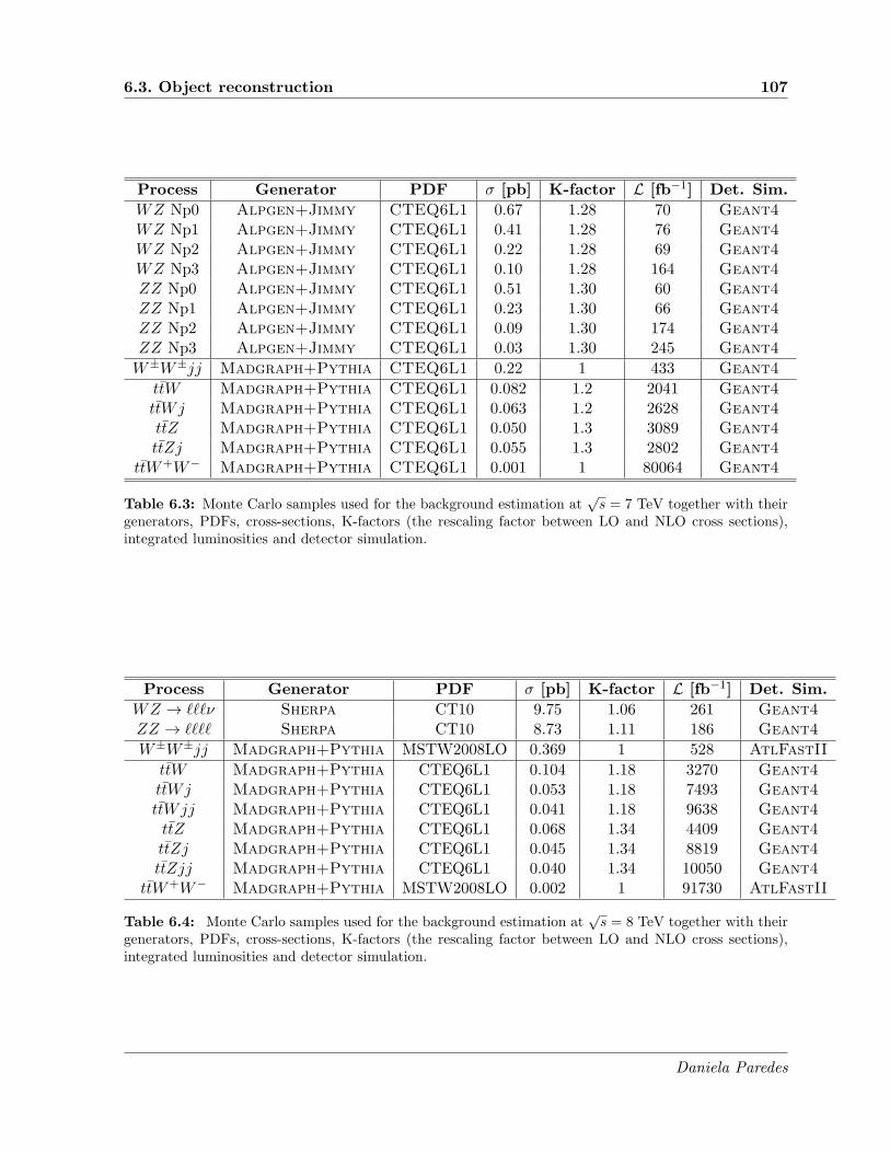
6.3. Object reconstruction 107
Process Generator PDF σ [pb] K-factor L [fb−1] Det. Sim.
WZ Np0 Alpgen+Jimmy CTEQ6L1 0.67 1.28 70 Geant4
WZ Np1 Alpgen+Jimmy CTEQ6L1 0.41 1.28 76 Geant4
WZ Np2 Alpgen+Jimmy CTEQ6L1 0.22 1.28 69 Geant4
WZ Np3 Alpgen+Jimmy CTEQ6L1 0.10 1.28 164 Geant4
ZZ Np0 Alpgen+Jimmy CTEQ6L1 0.51 1.30 60 Geant4
ZZ Np1 Alpgen+Jimmy CTEQ6L1 0.23 1.30 66 Geant4
ZZ Np2 Alpgen+Jimmy CTEQ6L1 0.09 1.30 174 Geant4
ZZ Np3 Alpgen+Jimmy CTEQ6L1 0.03 1.30 245 Geant4
W±W±jj Madgraph+Pythia CTEQ6L1 0.22 1 433 Geant4
ttW Madgraph+Pythia CTEQ6L1 0.082 1.2 2041 Geant4
ttWj Madgraph+Pythia CTEQ6L1 0.063 1.2 2628 Geant4
ttZ Madgraph+Pythia CTEQ6L1 0.050 1.3 3089 Geant4
ttZj Madgraph+Pythia CTEQ6L1 0.055 1.3 2802 Geant4
ttW+W− Madgraph+Pythia CTEQ6L1 0.001 1 80064 Geant4
Table 6.3: Monte Carlo samples used for the background estimation at√s = 7 TeV together with their
generators, PDFs, cross-sections, K-factors (the rescaling factor between LO and NLO cross sections),integrated luminosities and detector simulation.
Process Generator PDF σ [pb] K-factor L [fb−1] Det. Sim.
WZ → ℓℓℓν Sherpa CT10 9.75 1.06 261 Geant4
ZZ → ℓℓℓℓ Sherpa CT10 8.73 1.11 186 Geant4
W±W±jj Madgraph+Pythia MSTW2008LO 0.369 1 528 AtlFastII
ttW Madgraph+Pythia CTEQ6L1 0.104 1.18 3270 Geant4
ttWj Madgraph+Pythia CTEQ6L1 0.053 1.18 7493 Geant4
ttWjj Madgraph+Pythia CTEQ6L1 0.041 1.18 9638 Geant4
ttZ Madgraph+Pythia CTEQ6L1 0.068 1.34 4409 Geant4
ttZj Madgraph+Pythia CTEQ6L1 0.045 1.34 8819 Geant4
ttZjj Madgraph+Pythia CTEQ6L1 0.040 1.34 10050 Geant4
ttW+W− Madgraph+Pythia MSTW2008LO 0.002 1 91730 AtlFastII
Table 6.4: Monte Carlo samples used for the background estimation at√s = 8 TeV together with their
generators, PDFs, cross-sections, K-factors (the rescaling factor between LO and NLO cross sections),integrated luminosities and detector simulation.
Daniela Paredes

108 Chapter 6. Data and event preselection
• Jets: They are reconstructed in the calorimeter from topological clusters2 using the anti-ktalgorithm [142] with a radius R = 0.4, and calibrated to the hadronic energy scale usingpT- and η-dependent corrections
3. They are required to have pT > 25 GeV and |η| < 2.5.In order to avoid reconstructing electrons as jets, the closest jet within a cone of radius∆R(jet, e) = 0.2 from an electron passing the electron selection quality cuts is removed(both probably correspond to the same object). Jets without any associated track are alsoaccepted. To reject events from pileup, a quantity called jet-vertex-fraction (JVF) has beenused. It corresponds to the ratio of the sum of the pT of all tracks, with pT > 0.4 GeV,within the jet that originate from the primary vertex associated with the hard-scatteringcollision, over the sum of the pT of all tracks matched to the jet. Jets selected have tosatisfy a |JVF| > 0.75 (resp. 0.5) at 7 (resp. 8) TeV.
• b-jets: There are different b-tagging algorithms in ATLAS. They exploit the fact that Bmesons have a long lifetime and can travel a few mm in the detector before decaying.This way, a certain number of tracks point to a secondary vertex instead of pointing to thereconstructed primary vertex. The impact parameters of these tracks are large. Thus, thereare algorithms based on the impact parameter (IP3D), on the secondary vertex (SV1) andon the decay chain reconstruction (JetFitter). A multivariate b-tagging algorithm [144] atan operating point of 70% efficiency for b-jets in tt events is used in this analysis to selectjets from the decay of heavy flavor hadrons. This is a neural network-based algorithmthat uses the output weights of IP3D, SV1 and JetFitter as inputs. The operating pointcorresponds to a mis-tag rate of less than 1%, as determined in simulated tt events.
• Electrons: Candidate electrons are identified by means of a shower in the EM calorimeterconsistent with expectation, as well as a good quality track pointing to the cluster in thecalorimeter. They are required to have a transverse energy ET > 25 GeV and satisfy theTight ATLAS electron criteria [145]. They have to fall in a well instrumented region of thedetector, i.e. |ηcluster| < 2.47, excluding the calorimeter transition region 1.37 < |ηcluster| <1.52. Isolation cuts are also imposed such that the efficiency of each isolation requirementis 90%. These cuts depend on the transverse energy in a cone ∆R = 0.2 around theelectron (E∆R=0.2
T ), and on the total transverse momentum of all tracks within ∆R = 0.3of the electron (p∆R=0.3
T ). At 7 (resp. 8) TeV, the values used in the cuts range from 1.4(resp. 1.08) GeV to 3.7 (resp. 2.7) GeV for E∆R=0.2
T , and from 1 (resp. 0.9) GeV to 1.05(resp. 1.15) GeV for p∆R=0.3
T . Electrons within a cone ∆R(e, jet) = 0.4 of a reconstructedjet are removed. At 8 TeV, the track is required to be consistent within 2 mm in z withthe reconstructed primary vertex of the event, and a hit in the innermost layer of the innerdetector is also required, for active modules, to reject electrons from conversions.
• Muons: Candidate muon tracks are required to be well measured in both the inner detectorand the muon spectrometer. They have to pass the ATLAS muon quality cuts [146].Muons are required to fall within |η| < 2.5 and to satisfy a pT > 20 (resp. 25) GeV at 7(resp. 8) TeV. As for the electrons, isolation cuts are also applied. At 7 TeV, they requirea transverse energy within a cone ∆R = 0.2 along the direction of the muon candidate to
2Topological clusters algorithm or topoclusters is one of the two different cells clustering algorithms used byATLAS. They are a dynamically formed combination of cells around seed cells that exceed a given signal-to-noiseratio threshold, and which are used as inputs for the jet reconstruction algorithm.
3The corrections are derived from collision and test-beam data as well as simulation [143].
Daniela Paredes

6.4. Preselection of events 109
be less than 4 GeV, and a total transverse momentum of all tracks within ∆R = 0.3 tobe less than 2.5 GeV. At 8 TeV, muon candidates are required to be isolated from othercentral track activity within a cone with radius that decreases with increasing muon pT:∆R = 0.4/(pT/10 GeV). The summed pT of all tracks (other than the muon track) inthat cone is required to be less than 5% of the muon pT. Muons are also required to have∆R(µ, jet) > 0.4 from any jet. Events with an electron candidate that shares a track witha muon candidate are rejected. Cosmic rejection of muons is also applied when the anglebetween two muons in the transverse plane satisfies ∆φ(µ1, µ2) > 3.1 rad.
• Missing transverse momentum (EmissT ): The Emiss
T reconstruction includes contri-butions from energy deposits in the calorimeters and muons reconstructed in the muonspectrometer as [147]:
Emissx(y) = Emiss,calo
x(y) + Emiss,µx(y) . (6.1)
It uses calorimeter cells calibrated according to the reconstructed physics object to whichthey are associated in a chosen order: electrons, photons, hadronically decaying τ -leptons,jets and muons. Cells not associated with any such objects are also taken into account(Emiss,CellOut
T ). Thus, the calorimeter term is computed as:
Emiss,calox(y) = Emiss,e
x(y) +Emiss,γx(y) +Emiss,τ
x(y) +Emiss,jetsx(y) +Emiss,softjets
x(y) +(Emiss,calo,µx(y) )+Emiss,CellOut
x(y) ,
(6.2)where each term is calculated from the negative sum of calibrated cell energies inside thecorresponding objects.
The EmissT muon term is computed from the momenta of the muon tracks reconstructed
with |η| < 2.7:
Emiss,µx(y) = −
∑
muons
pµx(y). (6.3)
6.4 Preselection of events
The preselection of events is based on the standard/quality selection applied for studies of topquark physics in ATLAS. It is applied basically to clean-up the samples and to select the eventscorresponding to the final state of the signal studied. In this analysis, the final state of four topquarks has to contain at least one lepton pair with the same electric charge, missing transversemomentum (Emiss
T ) due to the presence of neutrinos, and large jet multiplicity, including b-jets.All the selected events have to satisfy the following requirements:
1. Events in data are required to pass the 2011 (resp. 2012) Good Run List selection definedby the ATLAS Top Group for the data collected at
√s = 7 (resp. 8) TeV.
2. One primary vertex determined from at least five tracks, each with pT > 0.4 GeV, isrequired. If there are multiple vertices reconstructed, the vertex with the largest sum ofthe squared transverse momenta of its associated tracks is taken as the primary vertex.
3. Events with noise bursts and data integrity errors in the LAr and TileCal calorimeter arerejected.
Daniela Paredes

110 Chapter 6. Data and event preselection
4. For the analysis performed with the setup of√s = 7 TeV, events must contain at least two
isolated leptons of the same electric charge. In events with more than one same-sign pair,the pairs are sorted according to the leading lepton pT, then by the subleading lepton pT.The first pair is chosen. At
√s = 8 TeV, events with exactly two leptons of the same electric
charge are required. The leading lepton of the pair is required to have pT > 25 GeV. In thisstep of the analysis, the events are classified in three channels: ee, eµ and µµ, dependingon the selected lepton flavors.
5. At least one of the selected leptons must match the one that triggered the readout of theevent as shown in Table 6.1.
6. In the ee and µµ channels, the invariant mass of the selected leptons must exceed 15 GeVand be out of the Z-boson mass region, i.e. |mℓℓ −mZ | > 10 GeV.
7. At least two jets are required, including at least one b-tagged jet.
8. The missing transverse momentum must satisfy EmissT > 40 GeV.
9. The scalar sum of the pT of all leptons and jets, defined as HT is required to exceed350 GeV.
6.5 Discriminant variables
After the preselection, the discriminant variables were identified to be the number of jets (Njets),the number of b-jets (Nb−jets), the scalar sum of pT of all leptons and jets (HT), and the missingtransverse momentum (Emiss
T ). Their distributions are shown in Figs. 6.1, 6.2 and 6.3, for theee, eµ and µµ channels at
√s = 7 TeV, respectively. The distributions of these variables at√
s = 8 TeV can be seen in Figs. 6.4, 6.5 and 6.6. The distributions of the leading lepton pTand sub-leading lepton pT are also shown, together with the four tops signal for the contactinteraction. The cuts on Emiss
T and HT have been removed. These discriminant variables will beused to optimize the signal selection in Chapter 8.
Daniela Paredes

6.5. Discriminant variables 111
jetsN2 4 6 8 10 12 14 16 18 20
Events
-110
1
10Q Mis-id
Fakes
+Z/W(W)ttWZ/ZZ
±W±W
132.4)× C.I. (ttttUncertainty
=7 TeVsee channel, InternalATLAS-1
Ldt = 4.7 fb∫
b-jetsN0 2 4 6 8 10
Events
-110
1
10
Q Mis-id
Fakes
+Z/W(W)ttWZ/ZZ
±W±W
132.4)× C.I. (ttttUncertainty
=7 TeVsee channel, InternalATLAS-1
Ldt = 4.7 fb∫
[GeV]TH500 1000 1500 2000 2500 3000 3500
Events
/ 1
00 G
eV
-110
1
10 Q Mis-id
Fakes
+Z/W(W)ttWZ/ZZ
±W±W
132.4)× C.I. (ttttUncertainty
=7 TeVsee channel, InternalATLAS-1
Ldt = 4.7 fb∫
[GeV]miss
TE0 100 200 300 400 500 600 700 800 900 1000
Events
/ 4
0 G
eV
-110
1
10 Q Mis-id
Fakes
+Z/W(W)ttWZ/ZZ
±W±W
132.4)× C.I. (ttttUncertainty
=7 TeVsee channel, InternalATLAS-1
Ldt = 4.7 fb∫
[GeV]T
Leading lepton p0 100 200 300 400 500 600
Events
/ 4
0 G
eV
-110
1
10Q Mis-id
Fakes
+Z/W(W)ttWZ/ZZ
±W±W
132.4)× C.I. (ttttUncertainty
=7 TeVsee channel, InternalATLAS-1
Ldt = 4.7 fb∫
[GeV]T
Sub-leading lepton p0 50 100 150 200 250 300
Events
/ 4
0 G
eV
-110
1
10Q Mis-id
Fakes
+Z/W(W)ttWZ/ZZ
±W±W
132.4)× C.I. (ttttUncertainty
=7 TeVsee channel, InternalATLAS-1
Ldt = 4.7 fb∫
Figure 6.1: Distribution of the kinematical variables in the ee channel at√s = 7 TeV after preselection
removing the cut on EmissT and HT. The cross section of the signal is scaled up so that the signal integral
is equal to the background integral. The background histograms are stacked to show the total expectedbackground.
Daniela Paredes

112 Chapter 6. Data and event preselection
jetsN2 4 6 8 10 12 14 16 18 20
Events
-110
1
10
Q Mis-id
Fakes
+Z/W(W)ttWZ/ZZ
±W±W
93.3)× C.I. (ttttUncertainty
=7 TeVs channel, µe InternalATLAS-1
Ldt = 4.7 fb∫
b-jetsN0 2 4 6 8 10
Events
-110
1
10
210
Q Mis-id
Fakes
+Z/W(W)ttWZ/ZZ
±W±W
93.3)× C.I. (ttttUncertainty
=7 TeVs channel, µe InternalATLAS-1
Ldt = 4.7 fb∫
[GeV]TH500 1000 1500 2000 2500 3000 3500
Events
/ 1
00 G
eV
-110
1
10
Q Mis-id
Fakes
+Z/W(W)ttWZ/ZZ
±W±W
93.3)× C.I. (ttttUncertainty
=7 TeVs channel, µe InternalATLAS-1
Ldt = 4.7 fb∫
[GeV]miss
TE0 100 200 300 400 500 600 700 800 900 1000
Events
/ 4
0 G
eV
-110
1
10
Q Mis-id
Fakes
+Z/W(W)ttWZ/ZZ
±W±W
93.3)× C.I. (ttttUncertainty
=7 TeVs channel, µe InternalATLAS-1
Ldt = 4.7 fb∫
[GeV]T
Leading lepton p0 100 200 300 400 500 600
Events
/ 4
0 G
eV
-110
1
10
Q Mis-id
Fakes
+Z/W(W)ttWZ/ZZ
±W±W
93.3)× C.I. (ttttUncertainty
=7 TeVs channel, µe InternalATLAS-1
Ldt = 4.7 fb∫
[GeV]T
Sub-leading lepton p0 50 100 150 200 250 300
Events
/ 4
0 G
eV
-110
1
10
Q Mis-id
Fakes
+Z/W(W)ttWZ/ZZ
±W±W
93.3)× C.I. (ttttUncertainty
=7 TeVs channel, µe InternalATLAS-1
Ldt = 4.7 fb∫
Figure 6.2: Distribution of the kinematical variables in the eµ channel at√s = 7 TeV after preselection
removing the cut on EmissT and HT. The cross section of the signal is scaled up so that the signal integral
is equal to the background integral. The background histograms are stacked to show the total expectedbackground.
Daniela Paredes

6.5. Discriminant variables 113
jetsN2 4 6 8 10 12 14 16 18 20
Events
-110
1
10Fakes
+Z/W(W)ttWZ/ZZ
±W±W 58.7)× C.I. (tttt
Uncertainty
=7 TeVs channel, µµ InternalATLAS-1
Ldt = 4.7 fb∫
b-jetsN0 2 4 6 8 10
Events
-110
1
10
Fakes
+Z/W(W)ttWZ/ZZ
±W±W 58.7)× C.I. (tttt
Uncertainty
=7 TeVs channel, µµ InternalATLAS-1
Ldt = 4.7 fb∫
[GeV]TH500 1000 1500 2000 2500 3000 3500
Events
/ 1
00 G
eV
-110
1
10 Fakes
+Z/W(W)ttWZ/ZZ
±W±W 58.7)× C.I. (tttt
Uncertainty
=7 TeVs channel, µµ InternalATLAS-1
Ldt = 4.7 fb∫
[GeV]miss
TE0 100 200 300 400 500 600 700 800 900 1000
Events
/ 4
0 G
eV
-110
1
10 Fakes
+Z/W(W)ttWZ/ZZ
±W±W 58.7)× C.I. (tttt
Uncertainty
=7 TeVs channel, µµ InternalATLAS-1
Ldt = 4.7 fb∫
[GeV]T
Leading lepton p0 100 200 300 400 500 600
Events
/ 4
0 G
eV
-110
1
10 Fakes
+Z/W(W)ttWZ/ZZ
±W±W 58.7)× C.I. (tttt
Uncertainty
=7 TeVs channel, µµ InternalATLAS-1
Ldt = 4.7 fb∫
[GeV]T
Sub-leading lepton p0 50 100 150 200 250 300
Events
/ 4
0 G
eV
-110
1
10
Fakes
+Z/W(W)ttWZ/ZZ
±W±W 58.7)× C.I. (tttt
Uncertainty
=7 TeVs channel, µµ InternalATLAS-1
Ldt = 4.7 fb∫
Figure 6.3: Distribution of the kinematical variables in the µµ channel at√s = 7 TeV after preselection
removing the cut on EmissT and HT. The cross section of the signal is scaled up so that the signal integral
is equal to the background integral. The background histograms are stacked to show the total expectedbackground.
Daniela Paredes

114 Chapter 6. Data and event preselection
jetsN2 4 6 8 10 12 14 16 18 20
Events
-110
1
10
Q Mis-id
Fakes
+Z/W(W)ttWZ/ZZ
±W±W
65.3)× C.I. (ttttUncertainty
=8 TeVsee channel, InternalATLAS-1
Ldt = 14.3 fb∫
b-jetsN0 2 4 6 8 10
Events
-110
1
10
210
Q Mis-id
Fakes
+Z/W(W)ttWZ/ZZ
±W±W
65.3)× C.I. (ttttUncertainty
=8 TeVsee channel, InternalATLAS-1
Ldt = 14.3 fb∫
[GeV]TH500 1000 1500 2000 2500 3000 3500
Events
/ 1
00 G
eV
-110
1
10
Q Mis-id
Fakes
+Z/W(W)ttWZ/ZZ
±W±W
65.3)× C.I. (ttttUncertainty
=8 TeVsee channel, InternalATLAS-1
Ldt = 14.3 fb∫
[GeV]miss
TE0 100 200 300 400 500 600 700 800 900 1000
Events
/ 4
0 G
eV
-110
1
10
210
Q Mis-id
Fakes
+Z/W(W)ttWZ/ZZ
±W±W
65.3)× C.I. (ttttUncertainty
=8 TeVsee channel, InternalATLAS-1
Ldt = 14.3 fb∫
[GeV]T
Leading lepton p0 100 200 300 400 500 600
Events
/ 4
0 G
eV
-110
1
10
210
Q Mis-id
Fakes
+Z/W(W)ttWZ/ZZ
±W±W
65.3)× C.I. (ttttUncertainty
=8 TeVsee channel, InternalATLAS-1
Ldt = 14.3 fb∫
[GeV]T
Sub-leading lepton p0 50 100 150 200 250 300
Events
/ 4
0 G
eV
-110
1
10
210
Q Mis-id
Fakes
+Z/W(W)ttWZ/ZZ
±W±W
65.3)× C.I. (ttttUncertainty
=8 TeVsee channel, InternalATLAS-1
Ldt = 14.3 fb∫
Figure 6.4: Distribution of the kinematical variables in the ee channel at√s = 8 TeV after preselection
removing the cut on EmissT and HT . The cross section of the signal is scaled up so that the signal integral
is equal to the background integral. The background histograms are stacked to show the total expectedbackground.
Daniela Paredes

6.5. Discriminant variables 115
jetsN2 4 6 8 10 12 14 16 18 20
Events
-110
1
10
210
Q Mis-id
Fakes
+Z/W(W)ttWZ/ZZ
±W±W
32.1)× C.I. (ttttUncertainty
=8 TeVs channel, µe InternalATLAS-1
Ldt = 14.3 fb∫
b-jetsN0 2 4 6 8 10
Events
-110
1
10
210Q Mis-id
Fakes
+Z/W(W)ttWZ/ZZ
±W±W
32.1)× C.I. (ttttUncertainty
=8 TeVs channel, µe InternalATLAS-1
Ldt = 14.3 fb∫
[GeV]TH500 1000 1500 2000 2500 3000 3500
Events
/ 1
00 G
eV
-110
1
10
210
Q Mis-id
Fakes
+Z/W(W)ttWZ/ZZ
±W±W
32.1)× C.I. (ttttUncertainty
=8 TeVs channel, µe InternalATLAS-1
Ldt = 14.3 fb∫
[GeV]miss
TE0 100 200 300 400 500 600 700 800 900 1000
Events
/ 4
0 G
eV
-110
1
10
210
Q Mis-id
Fakes
+Z/W(W)ttWZ/ZZ
±W±W
32.1)× C.I. (ttttUncertainty
=8 TeVs channel, µe InternalATLAS-1
Ldt = 14.3 fb∫
[GeV]T
Leading lepton p0 100 200 300 400 500 600
Events
/ 4
0 G
eV
-110
1
10
210
Q Mis-id
Fakes
+Z/W(W)ttWZ/ZZ
±W±W
32.1)× C.I. (ttttUncertainty
=8 TeVs channel, µe InternalATLAS-1
Ldt = 14.3 fb∫
[GeV]T
Sub-leading lepton p0 50 100 150 200 250 300
Events
/ 4
0 G
eV
-110
1
10
210Q Mis-id
Fakes
+Z/W(W)ttWZ/ZZ
±W±W
32.1)× C.I. (ttttUncertainty
=8 TeVs channel, µe InternalATLAS-1
Ldt = 14.3 fb∫
Figure 6.5: Distribution of the kinematical variables in the eµ channel at√s = 8 TeV after preselection
removing the cut on EmissT and HT . The cross section of the signal is scaled up so that the signal integral
is equal to the background integral. The background histograms are stacked to show the total expectedbackground.
Daniela Paredes

116 Chapter 6. Data and event preselection
jetsN2 4 6 8 10 12 14 16 18 20
Events
-110
1
10
Fakes
+Z/W(W)ttWZ/ZZ
±W±W 14.8)× C.I. (tttt
Uncertainty
=8 TeVs channel, µµ InternalATLAS-1
Ldt = 14.3 fb∫
b-jetsN0 2 4 6 8 10
Events
-110
1
10
210
Fakes
+Z/W(W)ttWZ/ZZ
±W±W 14.8)× C.I. (tttt
Uncertainty
=8 TeVs channel, µµ InternalATLAS-1
Ldt = 14.3 fb∫
[GeV]TH500 1000 1500 2000 2500 3000 3500
Events
/ 1
00 G
eV
-110
1
10
Fakes
+Z/W(W)ttWZ/ZZ
±W±W 14.8)× C.I. (tttt
Uncertainty
=8 TeVs channel, µµ InternalATLAS-1
Ldt = 14.3 fb∫
[GeV]miss
TE0 100 200 300 400 500 600 700 800 900 1000
Events
/ 4
0 G
eV
-110
1
10
Fakes
+Z/W(W)ttWZ/ZZ
±W±W 14.8)× C.I. (tttt
Uncertainty
=8 TeVs channel, µµ InternalATLAS-1
Ldt = 14.3 fb∫
[GeV]T
Leading lepton p0 100 200 300 400 500 600
Events
/ 4
0 G
eV
-110
1
10
Fakes
+Z/W(W)ttWZ/ZZ
±W±W 14.8)× C.I. (tttt
Uncertainty
=8 TeVs channel, µµ InternalATLAS-1
Ldt = 14.3 fb∫
[GeV]T
Sub-leading lepton p0 50 100 150 200 250 300
Events
/ 4
0 G
eV
-110
1
10
Fakes
+Z/W(W)ttWZ/ZZ
±W±W 14.8)× C.I. (tttt
Uncertainty
=8 TeVs channel, µµ InternalATLAS-1
Ldt = 14.3 fb∫
Figure 6.6: Distribution of the kinematical variables in the µµ channel at√s = 8 TeV after preselection
removing the cut on EmissT and HT . The cross section of the signal is scaled up so that the signal integral
is equal to the background integral. The background histograms are stacked to show the total expectedbackground.
Daniela Paredes

Chapter 7
Background estimation
Contents
7.1 Introduction . . . . . . . . . . . . . . . . . . . . . . . . . . . . . . . . . . . . . 117
7.2 Irreducible background . . . . . . . . . . . . . . . . . . . . . . . . . . . . . . . 118
7.3 False same-sign dilepton pairs . . . . . . . . . . . . . . . . . . . . . . . . . . . 118
7.3.1 Mis-reconstructed leptons . . . . . . . . . . . . . . . . . . . . . . . . . . . . . . 119
7.3.2 Mis-identification of the electron charge . . . . . . . . . . . . . . . . . . . . . . 123
7.3.3 Overlap between the electron charge mis-identification and fake electrons . . . 135
7.4 Background validation . . . . . . . . . . . . . . . . . . . . . . . . . . . . . . . 137
7.4.1 Control regions at√s = 7 TeV . . . . . . . . . . . . . . . . . . . . . . . . . . . 137
7.4.2 Control regions at√s = 8 TeV . . . . . . . . . . . . . . . . . . . . . . . . . . . 150
7.1 Introduction
Several SM processes can mimic the final state of four top quarks. In particular, for a finalstate with two leptons of the same electric charge, the contribution of the SM processes with twopromptly produced same-sign leptons is very small, since this kind of events is rarely produced inthe SM. The main contribution is coming from the instrumental backgrounds, where the objectsare mis-identified or mis-reconstructed. This way, the background can be divided into two maincategories:
• Irreducible background.
• False same-sign dilepton pairs.
The irreducible background is estimated from simulated samples, while the backgroundcoming from false same-sign dilepton pairs is estimated from data. Both sources of backgroundare validated in control regions which are orthogonal to the signal selection.
Daniela Paredes

118 Chapter 7. Background estimation
This chapter is dedicated to give a full description of the background estimation. Thesources of irreducible background are discussed in Section 7.2. The sources and estimation ofthe background coming from false same-sign dilepton pairs are presented in Section 7.3. Finally,the validation of the background is given in Section 7.4.
7.2 Irreducible background
This kind of background corresponds to Standard Model processes with real same-sign dileptonpairs. The dominant process contributing (see cross-section production in Table 6.3 and 6.4) isthe diboson production, WZ and ZZ, where both gauge bosons decay leptonically as
W±Z → ℓ±νℓ+ℓ−, (7.1)
ZZ → ℓ+ℓ−ℓ+ℓ−. (7.2)
Less significant contributions are coming from production of like-sign W bosons in associationwith two jets, and from associated production of tt pairs with a W or Z boson as
W±W±jj → ℓ±νℓ±νjj, (7.3)
ttW± → W+bW−bW±
→ ℓ+νbjjbℓ±ν, jjbℓ−νbℓ±ν or ℓ+νbℓ−νbℓ±ν, (7.4)
ttZ → W+bW−bZ
→ ℓ+νbjjbℓ+ℓ−, jjbℓ−νbℓ+ℓ− or ℓ+νbℓ−νbℓ+ℓ−. (7.5)
A last and almost negligible contribution comes from the production of ttW+W− events as
ttW+W− → W+bW−bW+W− (7.6)
→ ℓ+νbjjbℓ+νjj, ℓ+νbℓ−νbℓ+νjj, ℓ+νbjjbℓ+νℓ−ν, ℓ+νbℓ−νbℓ+νℓ−ν,
jjbℓ−νbjjℓ−ν or jjbℓ−νbℓ+νℓ−ν. (7.7)
Each one of these processes is illustrated in Fig. 7.1. As stated before, this backgroundis estimated from simulated samples. The Monte Carlo samples together with their generatorswere already detailed in Section 6.2.2.2. Background coming from tbZ + jets and multi partoninteractions giving same-sign dibosons and jets have been neglected.
7.3 False same-sign dilepton pairs
This background corresponds to physics processes which do not give same-sign dilepton events,but are reconstructed as such. It comes from:
• Mis-reconstructed leptons: At least one of the two leptons in the selected same-signpair is not a real isolated lepton but has been reconstructed as such.
• Mis-identification of the electron charge: The sign of the electric charge of one ofthe two leptons in the selected same-sign pair has been mis-reconstructed, leading to atrue opposite-sign lepton pair being reconstructed as a same-sign pair. The charge mis-identification of muons is much smaller (around 107 smaller [148]) and has therefore beenneglected in this analysis.
Daniela Paredes

7.3. False same-sign dilepton pairs 119
g u
u
d
W+
d Z
(a)
u
u
Z
Z
(b)
u
u
d
W+
d
W+
d
d
(c)
u
t
d
W+
d
t
(d)
g d
t
dZd
dt
(e)
g
g
t
t
t
b
W+
tW−
(f)
Figure 7.1: Examples of Feynman diagrams illustrating the WZ (a), ZZ (b), W±W±jj (c), ttW (d),ttZ (e) and ttW+W− (f) productions.
These two sources of background are estimated using data-driven techniques and not usingMonte Carlo samples. These techniques are explained below.
7.3.1 Mis-reconstructed leptons
The fake leptons1 constitute the largest SM background source. It includes all the processeswhere at least one of the leptons in the pair is non-prompt. The dominant contribution comesfrom W + jets and QCD multijet (including bb and cc), with smaller contributions from Z+ jetsand tt production.
There are several sources for this background depending on the lepton type. For electrons,a fake lepton may arise from a photon conversion, from a heavy flavor decay, or a light flavor jetwith a leading π0 overlapping with a charged particle. For muons, the dominant mechanism forthe creation of fake leptons is the semi-leptonic decay of a heavy flavor hadron, where a muonsurvives the isolation requirement.
To estimate this background, two sets of lepton selection criteria are defined, named looseand tight. The tight lepton definition is the same as in the analysis as detailed in Section 6.3, andit has to be a subset of the loose definition. The anti-tight lepton is defined to be an exclusivelyloose lepton, i.e. required not to be tight. The probabilities r and f that a real or fake looselepton passes the tight criteria are measured using purified control regions and they depend on thecharacteristics of the event. The matrix method [149, 150] is then used to estimate the numberof events in the signal region with at least one fake lepton.
The matrix method is discussed in Section 7.3.1.1. The evaluation of the probabilities rand f for the analysis performed with the data taken at
√s = 7 TeV and 8 TeV is given in
1“Fake leptons” include real leptons that are non-prompt.
Daniela Paredes

120 Chapter 7. Background estimation
Sections 7.3.1.2, and 7.3.1.3, respectively. The values of r and f for both, electrons and muons,were estimated by the Top Fakes Group2. At 7 (resp. 8) TeV, the events were weighted byLPNHE (resp. Arizona) group3.
7.3.1.1 Matrix method
In the matrix method, the number of events that contain two tight leptons is denoted NTT . Thenumber of events with one tight and one anti-tight is denoted NTA or NAT , distinguished bypT -ordering. Similarly, the two anti-tight lepton count is referred to as NAA. The total numberof events with two loose leptons is therefore N ll = NTT +NTA +NAT +NAA.
N llRR is the number of events that contain two real leptons, the number of events with
one real and one fake leptons is denoted N llRF or N ll
FR depending on the pT of the leptons, andthe number for two fake leptons is N ll
FF . The total number of events with two loose leptons istherefore N ll = N ll
RR +N llRF +N ll
FR +N llFF . These numbers are unknown.
The number of events with two tight leptons, in the signal region sample, can be written asNTT = N tt
RR+N ttRF +N tt
FR+N ttFF and the final fake estimation is N fakes
TT = r1f2NllRF +f1r2N
llFR+
f1f2NllFF , where r1 and f1 are the probabilities for the first lepton, and r2 and f2 for the second
lepton.Linear expressions are obtained for the observed yields NTT,TA,AT,AA as a function of the
unknown numbers N llRR,RF,FR,FF and the measured rates r and f . These linear expressions form
a matrix that is inverted to extract the real and fake content of the selected dilepton eventsample:
NTT
NTA
NAT
NAA
=
r1r2 r1f2 f1r2 f1f2r1(1− r2) r1(1− f2) f1(1− r2) f1(1− f2)(1− r1)r2 (1− r1)f2 (1− f1)r2 (1− f1)f2
(1− r1)(1− r2) (1− r1)(1− f2) (1− f1)(1− r2) (1− f1)(1− f2)
N llRR
N llRF
N llFR
N llFF
(7.8)In terms of real and fake leptons within the loose selection, the sum of the fake contribution
to the tight event selection is
N fakesTT = r1f2N
LLRF + f1r2N
LLFR + f1f2N
LLFF , (7.9)
= αr1f2[(f1 − 1)(1− r2)NTT + (1− f1)r2N
TA + f1(1− r2)NAT − f1r2N
AA] +
αf1r2[(r1 − 1)(1− f2)NTT + (1− r1)f2N
TA + r1(1− f2)NAT − r1f2N
AA] +
αf1f2[(1− r1)(1− r2)NTT + (r1 − 1)r2N
TA + r1(r2 − 1)NAT − r1r2NAA],
where
α =1
(r1 − f1)(r2 − f2). (7.10)
7.3.1.2 Estimation of the rates r and f at√s = 7 TeV
As said earlier, the tight lepton definitions are the same as in the analysis. The loose electronselection is equivalent to the tight electron selection with the isolation requirement replaced by
2The Top Fakes Group is an ATLAS internal group specialized in the computation of the background comingfrom fake leptons.
3The author of this thesis does not have any contribution to the computation of this background.
Daniela Paredes

7.3. False same-sign dilepton pairs 121
a looser cut, and looser quality requirements. The loose muon selection is equivalent to thetight muon selection with the isolation requirement removed. Loose muons close to a jet with a∆R(µ, jet) < 0.4 are removed.
The way in which the values of r and f have been computed for the analysis at√s = 7 TeV
for both, electrons and muons, based on the previous definitions of loose and tight, is describedas follows:
• Electrons: for computing the value of r, a highly purified sample of Z bosons was chosenin order to create a control region rich in real electrons. Thus the value of r was estimatedwith a tag-and-probe method on a sample Z → e+e− events. The Z sample was createdby asking for one tight electron (tag electron) and one loose electron (probe electron).Different background subtraction methods based on the Z-peak were applied: removal ofsame-sign events from opposite sign events in the signal region, side-band method on same-sign events, fit using a model for the signal and for the background components. The mainsystematic uncertainties are coming from the contamination of the sample of probe electronsby background: variations based in different signal regions and different fit ranges wereused to extract the background with the three different methods. A procedure using thedifferent variations has been developed in order to define the baseline selection. It consists ofconsidering the central value and the statistical uncertainty of an efficiency measurementas the averages of these quantities among all the variations of this measurement. Thesystematic uncertainty is then given by the spread of all variations.
For fake electrons, f was estimated in a sample with at least one jet, and exactly one looseelectron. A cut on the distance between the leading jet and the lepton is also applied∆R(leading jet, e) ≥ 0.7. Overlap removal is performed between electrons and jets usingthe loose leptons. The efficiency was measured in a control region with Emiss
T ≤ 20 GeVin order to enrich the sample in multijets. Contamination from signal leptons from Wand Z decays is still present in the low Emiss
T region, for that reason a higher purity ofthe sample is required. This is managed by correcting the number of observed loose andtight events in data based on Monte Carlo. A first systematic uncertainty is obtained byvarying the Emiss
T region from 15 GeV to 25 GeV. The fake efficiency is measured for thedifferent components of the background of signal leptons, which is made mostly from fakeleptons from light flavor jets, leptons from heavy flavor jets and photon conversion. Theseefficiencies are combined to get the central efficiency in the signal region and the systematicuncertainty.
Both real and fake efficiencies are parametrized as a function of |η| and electron pT.
• Muons: the efficiencies for muons were determined for two different data taking periods:The first period (BK) goes from March 2011 to August 2011 and gives stable results, whilethe second period (LM) goes from September 2011 to the end of the same year and givesresults slightly different due to the pile-up effect.
As for real electrons, the value of r for real muons was estimated using the tag-and-probemethod on the sample Z → µ+µ−, requiring events with one tight muon (tag muon) andone loose muon (probe muon).
The efficiencies for fake muons were optimized for tt → µ+ jets events. The fakes controlregion was chosen to be orthogonal to tt → µ + jets, and created by requiring one loose
Daniela Paredes

122 Chapter 7. Background estimation
muon. The fake efficiencies have been determined in a low transverse W mass regionmT(W ) < 20 GeV4 with an additional inverted triangular cut Emiss
T +mT(W ) < 60 GeV.The contribution from W + jets and Z + jets in the control region was subtracted in orderto obtain a more pure QCD estimate.
The fake and real efficiencies are a function of the muon |η| and pT of the leading jet inorder to take into account for dependencies on muon detector acceptance and hadronicactivity from hard jets affecting the muon isolation.
7.3.1.3 Estimation of the rates r and f at√s = 8 TeV
As in the previous case, the tight leptons are required to satisfy all of the selection criteria as forthe analysis. The loose electron selection is similar to the tight selection with the identificationcriteria relaxed and the isolation requirement removed. The loose muon selection is defined byremoving the isolation requirement if the muon pT is greater than 37 GeV, and requiring thesum of all track pT’s in a cone of R = 0.2 around the muon to be less than 0.12 times the muonspT otherwise. In both cases, the real and fake efficiencies are measured in samples with at leastone jet and exactly one loose lepton.
• Electrons: the real efficiencies r are measured in a dedicated control region, enriched withreal electrons. This way, they are determined in events with Emiss
T > 120 GeV.
The efficiencies for fake electrons are measured in a region with a low amount of EmissT . The
contamination of events with real electrons is removed using simulated events passing thefake control region cuts. Thus, the fake efficiencies are evaluated in events with Emiss
T <20 GeV or Emiss
T +mT(W ) < 60 GeV.
The fake and real efficiencies for electrons are parametrized as a function of different vari-ables: |η| and lepton pT, ∆φ between the electron and the Emiss
T vector, ∆R between theelectron and the jets,
∑
ET and EmissT .
• Muons: the efficiencies for a real muon passing the tight requirements are measured inevents with mT(W ) > 100 GeV.
Fake efficiencies for muons are determined from events where the impact parameter d0 ofthe muon with respect to the primary vertex was more than five standard deviations fromzero, i.e. |dsig0 | > 5. As for electrons, the contribution of events with real muons in thisregion is extracted using Monte Carlo samples.
The efficiencies are a function of muon η and pT, ∆R between the muon and the closestjet and the number of b-tagged jets in the event.
7.3.1.4 Yield measurement
In order to measure the yield of events with at least one fake lepton, the same selection of eventsthat will be estimated for the signal region has to be applied, but requiring loose leptons insteadof tight leptons. Then the efficiencies r and f are applied to these events as expressed by Eq. 7.9.
4The transverse mass is defined as mT =√
2pTEmissT (1− cos∆φ), where pT is the transverse momentum of the
charged lepton and ∆φ is the azimuthal angle between the charged lepton and the missing transverse momentum.
Daniela Paredes

7.3. False same-sign dilepton pairs 123
At 7 TeV, uncertainties on the estimate of background coming from fake leptons are 50% forthe ee channel, 40% for the eµ channel, and 30% for the µµ channel. At 8 TeV, the uncertaintieswere determined to be 30% in all channels (see Chapter 8).
7.3.2 Mis-identification of the electron charge
Opposite-sign leptons from SM processes as Drell-Yan, W+W−, and mainly tt, could contributeto the same-sign dilepton background if the charge of one of the leptons coming from the dilep-tonic decay of these processes is mis-measured.
There are two main sources of electron charge mis-identification:
• Hard Bremsstrahlung producing trident electrons (e± → e±γ∗ → e±e+e−) whose EMcluster is identified with the wrong electron’s track, leading to a mis-identification of thecharge. This source represents the main contribution to the background. The fraction oftrident electrons depends on the amount of material that the electrons traverse. In thedetector, the distribution of the material depends on |η|. Therefore, a strong dependenceon |η| is expected in the mis-identification rates.
• A slightly curved track that induces a measurement error. This effect is important at hightransverse momentum. Thus, a small dependence on electron pT is also expected in themis-identification rates.
As said before, for muons this background is negligible compared to other backgroundprocesses, and therefore is not considered in the analysis5.
The main strategy to estimate this background together with some preliminary conceptsto compute the mis-identification rates of the electron charge are presented in Section 7.3.2.1.The estimation of the rates in simulated samples is presented in Section 7.3.2.2. The differentmethods used to measure these rates in data are given in Section 7.3.2.3. Finally, the estimationof the rates for the different analyses at
√s = 7 TeV and 8 TeV are presented in Sections 7.3.2.4
and 7.3.2.5, respectively.
7.3.2.1 Main strategy and preliminary concepts
When a true opposite-sign event (for example tt → bW+bW− → bbe+e−νν) is produced, andassuming that ǫ is the rate of charge mis-identification for a single electron, there are threepossibilities for this event to be reconstructed:
1. e+e− +X without any charge mis-identification, with a probability of (1− ǫ)2,
2. e+e− +X with the two electrons having a charge flip, with a probability of ǫ2,
3. e±e±+X when only one of the two electrons is mis-identified, with a probability of 2ǫ(1−ǫ).
Therefore, if there are N true opposite-sign events, the reconstructed events will be:
• Nos = (1− 2ǫ+ 2ǫ2)N opposite-sign events,
5The rate of charge mis-identification for muons is only affected by the track curvature. Because of the longlever arm to the muon system and the fact that the charge is measured in both the inner detector and muonspectrometer the mis-identification rates of the muon charge are very low, making this background negligiblecompared to the other sources of background.
Daniela Paredes

124 Chapter 7. Background estimation
• N ss = 2ǫ(1− ǫ)N ≃ 2ǫN same-sign events,
where the last approximation for N ss corresponds to the assumption that ǫ is very small.
Knowing this charge mis-identification rate ǫ, it is therefore possible to compute the esti-mated number of same-sign events N ss from the measured number of opposite-sign events Nos,using the following expressions:
• N ss =ǫi+ǫj−2ǫiǫj
1−ǫi−ǫj+2ǫiǫjNos for the ee channel,
• N ss = ǫ1−ǫN
os for the eµ channel,
where ǫi and ǫj are the charge mis-identification rates for the two different electrons.
Finally, the method to estimate the number of same-sign events produced by the StandardModel true opposite-sign processes has two steps:
1. the measurement of the charge mis-identification rate ǫ,
2. the application of the measured rate to measured opposite-sign events Nos. The last onegives the estimation of N ss.
The mis-identification rates have been measured in a very clean sample of Z → e+e−,where the electrons fill the same requirements as the ones used in the analysis. They havebeen computed as a function of electron |η| (to be more precise, the full |η| range of the electronacceptance has been divided in regions, named bins, so that the rates are determined as a functionof |η| bins). In the analysis at
√s = 8 TeV, they have been corrected using a pT-dependent factor.
7.3.2.2 Estimation of the mis-identification rates of the electron charge in simulatedsamples: truth-matching
In simulated samples, the reconstructed electrons can be matched to the generated ones from theZ decay. A matching cone ∆R ≤ 0.2 is used to find reconstructed electrons that correspond totrue electrons produced from the Z decay6. The matching is done only to the electrons produceddirectly from the Z decay (primary electrons). It does not match reconstructed electrons toelectrons produced in the conversion of radiated photons from primary electrons, to electron-positron pairs, or to electrons produced in other secondary processes. If trident electrons, thereconstructed electrons are matched to the primary electron if the electrons produced in theconversion are almost collinear to the primary electron.
7.3.2.3 Estimation of the mis-identification rates of the electron charge in data
Different methods can be used to measure the mis-identification rates in data. These methodscan be also applied to compute the rates in simulated samples. Each one of these methods useselectrons coming from the leptonic decay of the Z boson. This way, the sample has been createdasking for exactly two electrons and no muons, where at least one of the selected leptons matchesthe corresponding trigger.
All the three methods studied here use Z signal events. Therefore, background comingfrom other processes where the dilepton invariant mass corresponds to the one of the Z boson
6It has been shown that for ∆R > 0.05, the size of the cone has no incidence on the matching performance [151].
Daniela Paredes

7.3. False same-sign dilepton pairs 125
needs to be subtracted. The background subtraction is done using a simple side-band method.This method consists in dividing the Z invariant mass in three regions, i.e. A, B and C, whereB is the central region corresponding to the Z peak. The number of events is counted in theregions on the sides of the peak, i.e. nA and nC , and removed from the total number of eventsin the peak region B, nB. This way, the number of signal events NZ is given by
NZ = nB − nA + nC2
. (7.11)
Once the background has been subtracted, the different methods can be applied to extractthe rates. They are explained below:
• Tag-and-probe: In the tag-and-probe method, the electrons are divided in two classes:tag and probe. In each pair, the tag electron is required to have a very low charge mis-identification rate. The sign of the other electron (probe electron) is the one under study.
As it will be shown later, the mis-identification rate of the electron charge in the centralregion of the detector is around two orders of magnitude lower than for electrons in theendcap regions. Therefore, the tag electrons are signal electrons with pseudorapidity withinthe interval established for the first |η| bin (the bin corresponding to the lowest value of|η|). At least one of the electrons in the pair must satisfy the tag condition. Otherwise,the event is rejected.
The number of same-sign Nss and opposite-sign Nos events in the Z peak is evaluatedbased on the |η| properties of the probe electron after background rejection. Thus, thecharge mis-identification rates are obtained as follows:
δie =N i
ss
N iss +N i
os
, (7.12)
where i corresponds to each bin in |η|. These values contain the mis-id rates of one tagand one probe electron. In order to obtain the charge flip for each lepton, the tag efficiencyneeds to be extracted. This way, for the first |η| bin 2 tag electrons are accepted. Therefore,the final charge mis-identification rate, ǫ, in this bin is computed as:
ǫ0 =δ0e2. (7.13)
For the remaining bins, the tag efficiency has to be computed as:
ǫi = δie − ǫ0, i 6= 0. (7.14)
• Direct extraction: in this method both electrons in the pair are required to be in thesame |η| bin. Otherwise the event is rejected. The charge flip is given by:
ǫi =N i
ss
2(N iss +N i
os), (7.15)
where N iss (N
ios) is the number of events in the Z peak with both same-sign (opposite-sign)
electrons in the same |η| bin i after background subtraction. The factor of 2 comes fromthe fact that the two electrons in the pair are in the same |η| bin.
Daniela Paredes
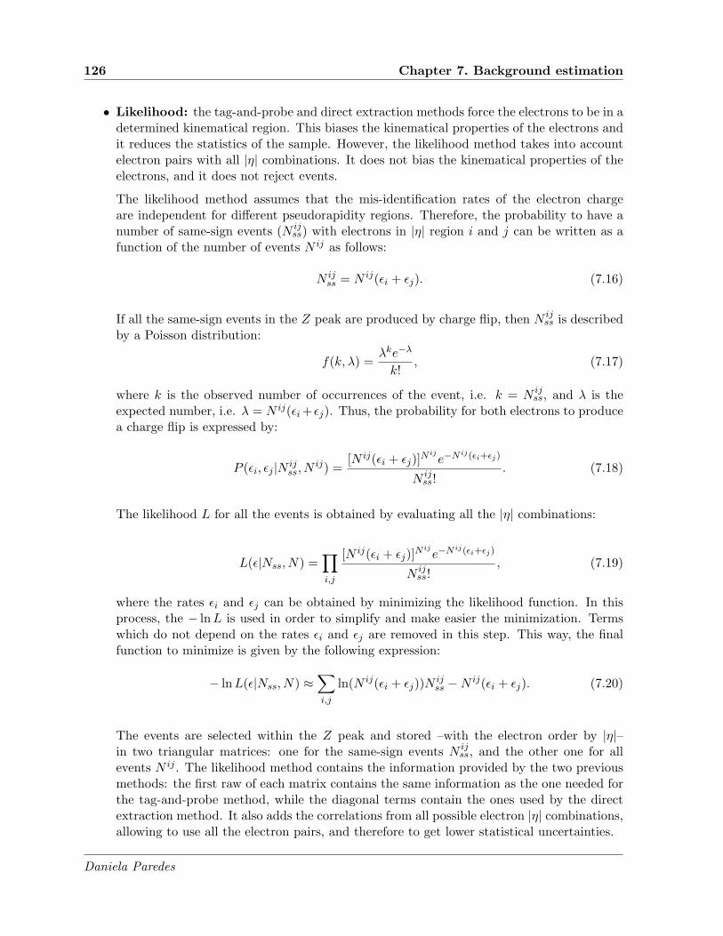
126 Chapter 7. Background estimation
• Likelihood: the tag-and-probe and direct extraction methods force the electrons to be in adetermined kinematical region. This biases the kinematical properties of the electrons andit reduces the statistics of the sample. However, the likelihood method takes into accountelectron pairs with all |η| combinations. It does not bias the kinematical properties of theelectrons, and it does not reject events.
The likelihood method assumes that the mis-identification rates of the electron chargeare independent for different pseudorapidity regions. Therefore, the probability to have anumber of same-sign events (N ij
ss) with electrons in |η| region i and j can be written as afunction of the number of events N ij as follows:
N ijss = N ij(ǫi + ǫj). (7.16)
If all the same-sign events in the Z peak are produced by charge flip, then N ijss is described
by a Poisson distribution:
f(k, λ) =λke−λ
k!, (7.17)
where k is the observed number of occurrences of the event, i.e. k = N ijss, and λ is the
expected number, i.e. λ = N ij(ǫi+ ǫj). Thus, the probability for both electrons to producea charge flip is expressed by:
P (ǫi, ǫj |N ijss, N
ij) =[N ij(ǫi + ǫj)]
N ij
e−N ij(ǫi+ǫj)
N ijss!
. (7.18)
The likelihood L for all the events is obtained by evaluating all the |η| combinations:
L(ǫ|Nss, N) =∏
i,j
[N ij(ǫi + ǫj)]N ij
e−N ij(ǫi+ǫj)
N ijss!
, (7.19)
where the rates ǫi and ǫj can be obtained by minimizing the likelihood function. In thisprocess, the − lnL is used in order to simplify and make easier the minimization. Termswhich do not depend on the rates ǫi and ǫj are removed in this step. This way, the finalfunction to minimize is given by the following expression:
− lnL(ǫ|Nss, N) ≈∑
i,j
ln(N ij(ǫi + ǫj))Nijss −N ij(ǫi + ǫj). (7.20)
The events are selected within the Z peak and stored –with the electron order by |η|–in two triangular matrices: one for the same-sign events N ij
ss, and the other one for allevents N ij . The likelihood method contains the information provided by the two previousmethods: the first raw of each matrix contains the same information as the one needed forthe tag-and-probe method, while the diagonal terms contain the ones used by the directextraction method. It also adds the correlations from all possible electron |η| combinations,allowing to use all the electron pairs, and therefore to get lower statistical uncertainties.
Daniela Paredes

7.3. False same-sign dilepton pairs 127
7.3.2.4 Estimation of the mis-identification rates at√s = 7 TeV
The rates of charge mis-identification for electrons were estimated as a function of the electron|η| for the three different methods as shown in Fig. 7.2(a), where they are denoted as ǫmis−id.The pT dependence of the rates was not considered in the analysis at
√s = 7 TeV. Differences
on the rates extracted from these methods come from the kinematic selection. The regions usedto subtract the background were defined as A ∈ [61, 81], B ∈ [81, 101] and C ∈ [101, 121].
|η|
0 0.5 1 1.5 2 2.5
mis
-id
∈
-410
-310
-210
-110
ATLAS Preliminary
= 7 TeVs
direct extraction
tag-and-probe
likelihood
(a)
[GeV]eem
60 70 80 90 100 110 120
# e
ve
nts
/Ge
V
0
100
200
300
400
500
600
700
800ATLAS Preliminary
= 7 TeVs
-1 Ldt = 4.7 fb∫
same-sign events
direct extraction
tag-and-probe
likelihood
(b)
Figure 7.2: a) Charge mis-identification rate as a function of the electron |η| b) Invariant mass distri-bution for same-sign and reweighed opposite-sign events around the Z-peak [18].
A closure test was performed by comparing the numbers of events selected in the Z-peakregion using same-sign electron pairs, and opposite-sign electron pairs reweighted by the mis-id weight depending on each method. These distributions are shown in Fig. 7.2(b). In thisfigure, the Z-peak for same-sign electrons is shifted to lower values with respect to opposite-signelectrons because a larger momentum fraction has been radiated for the same-sign case, dueto trident electrons. Around 5143 same-sign events are estimated in the Z-peak region. Thetag-and-probe method gives an under-estimation of the events with 3700 predicted events, whiledirect extraction predicts around 5500 events with an over-estimation. The likelihood methodgives the best agreement with 5000 events estimated. The differences on the rates estimation arewell-understood and come from the different kinematic requirements in the three methods. As aconsequence, the likelihood method was used to extract the nominal yield, while the other twomethods were used to estimate the systematic uncertainty. This background has been estimatedat 7 TeV by Saclay group7.
7Thanks to Lea Gauthier for producing these rates [148].
Daniela Paredes
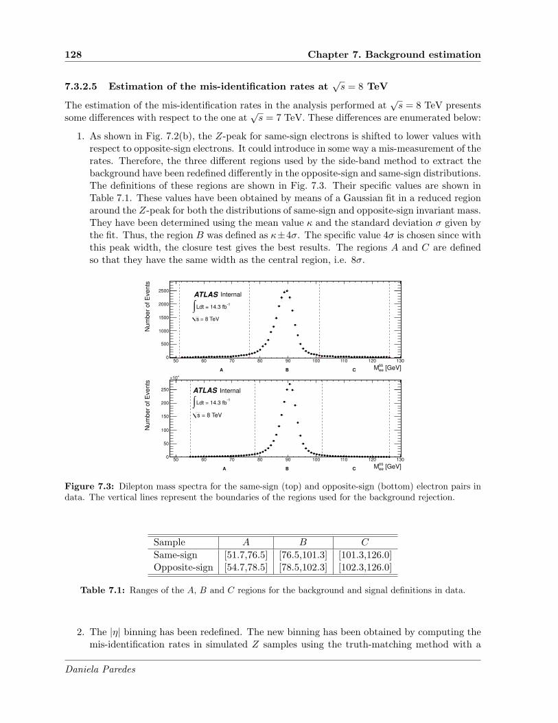
128 Chapter 7. Background estimation
7.3.2.5 Estimation of the mis-identification rates at√s = 8 TeV
The estimation of the mis-identification rates in the analysis performed at√s = 8 TeV presents
some differences with respect to the one at√s = 7 TeV. These differences are enumerated below:
1. As shown in Fig. 7.2(b), the Z-peak for same-sign electrons is shifted to lower values withrespect to opposite-sign electrons. It could introduce in some way a mis-measurement of therates. Therefore, the three different regions used by the side-band method to extract thebackground have been redefined differently in the opposite-sign and same-sign distributions.The definitions of these regions are shown in Fig. 7.3. Their specific values are shown inTable 7.1. These values have been obtained by means of a Gaussian fit in a reduced regionaround the Z-peak for both the distributions of same-sign and opposite-sign invariant mass.They have been determined using the mean value κ and the standard deviation σ given bythe fit. Thus, the region B was defined as κ±4σ. The specific value 4σ is chosen since withthis peak width, the closure test gives the best results. The regions A and C are definedso that they have the same width as the central region, i.e. 8σ.
[GeV]ss
eeM
50 60 70 80 90 100 110 120 130
Num
ber
of E
vents
0
500
1000
1500
2000
2500
A B C
-1Ldt = 14.3 fb∫ = 8 TeVs
ATLAS Internal
[GeV]os
eeM
50 60 70 80 90 100 110 120 130
Num
ber
of E
vents
0
50
100
150
200
250
310×
A B C
-1Ldt = 14.3 fb∫
ATLAS Internal
= 8 TeVs
Figure 7.3: Dilepton mass spectra for the same-sign (top) and opposite-sign (bottom) electron pairs indata. The vertical lines represent the boundaries of the regions used for the background rejection.
Sample A B C
Same-sign [51.7,76.5] [76.5,101.3] [101.3,126.0]Opposite-sign [54.7,78.5] [78.5,102.3] [102.3,126.0]
Table 7.1: Ranges of the A, B and C regions for the background and signal definitions in data.
2. The |η| binning has been redefined. The new binning has been obtained by computing themis-identification rates in simulated Z samples using the truth-matching method with a
Daniela Paredes
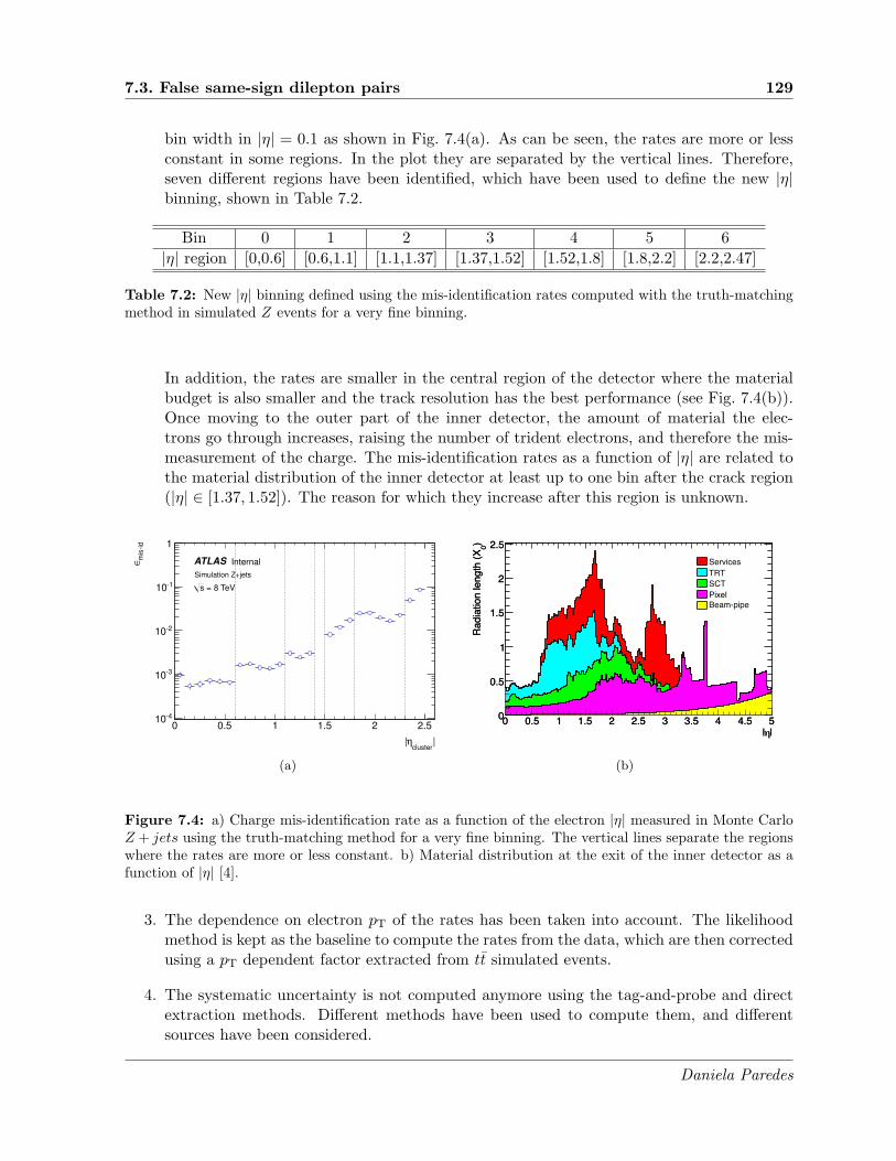
7.3. False same-sign dilepton pairs 129
bin width in |η| = 0.1 as shown in Fig. 7.4(a). As can be seen, the rates are more or lessconstant in some regions. In the plot they are separated by the vertical lines. Therefore,seven different regions have been identified, which have been used to define the new |η|binning, shown in Table 7.2.
Bin 0 1 2 3 4 5 6
|η| region [0,0.6] [0.6,1.1] [1.1,1.37] [1.37,1.52] [1.52,1.8] [1.8,2.2] [2.2,2.47]
Table 7.2: New |η| binning defined using the mis-identification rates computed with the truth-matchingmethod in simulated Z events for a very fine binning.
In addition, the rates are smaller in the central region of the detector where the materialbudget is also smaller and the track resolution has the best performance (see Fig. 7.4(b)).Once moving to the outer part of the inner detector, the amount of material the elec-trons go through increases, raising the number of trident electrons, and therefore the mis-measurement of the charge. The mis-identification rates as a function of |η| are related tothe material distribution of the inner detector at least up to one bin after the crack region(|η| ∈ [1.37, 1.52]). The reason for which they increase after this region is unknown.
|cluster
η|
0 0.5 1 1.5 2 2.5
mis
-id
∈
-410
-310
-210
-110
1
ATLAS Internal
Simulation Z+jets
= 8 TeVs
(a)
||0 0.5 1 1.5 2 2.5 3 3.5 4 4.5 5
)0
Ra
dia
tio
n le
ng
th (
X
0
0.5
1
1.5
2
2.5
||0 0.5 1 1.5 2 2.5 3 3.5 4 4.5 5
)0
Ra
dia
tio
n le
ng
th (
X
0
0.5
1
1.5
2
2.5
Services
TRT
SCT
Pixel
Beam-pipe
(b)
Figure 7.4: a) Charge mis-identification rate as a function of the electron |η| measured in Monte CarloZ + jets using the truth-matching method for a very fine binning. The vertical lines separate the regionswhere the rates are more or less constant. b) Material distribution at the exit of the inner detector as afunction of |η| [4].
3. The dependence on electron pT of the rates has been taken into account. The likelihoodmethod is kept as the baseline to compute the rates from the data, which are then correctedusing a pT dependent factor extracted from tt simulated events.
4. The systematic uncertainty is not computed anymore using the tag-and-probe and directextraction methods. Different methods have been used to compute them, and differentsources have been considered.
Daniela Paredes

130 Chapter 7. Background estimation
The last two points are developed in the next two sections. But before going to the pTcorrection it is necessary to validate the likelihood method. This is done by comparing the mis-identification rates computed with both likelihood and truth-matching methods on simulated Zevents. This comparison is shown in Fig. 7.5. As can be seen, the rates are compatible withinuncertainties.
mis
-id
∈
-410
-310
-210
-110
1
Likelihood
Truth-matching
ATLAS Preliminary
Simulation Z+jets
= 8 TeVs
|η|0 0.5 1 1.5 2 2.5
Lik
elih
oo
d/T
ruth
-ma
tch
ing
0.6
0.8
1
1.2
1.4
1.6
Figure 7.5: Comparison between the true and measured mis-identification rates as a function of |η| insimulated Z events.
All the simulated samples used in this section are detailed in Table 7.3.
Process Generator PDF Detector Simulation
Z → e+e− Np0 Alpgen+Pythia CTEQ6L1 Geant4
Z → e+e− Np1 Alpgen+Pythia CTEQ6L1 Geant4
Z → e+e− Np2 Alpgen+Pythia CTEQ6L1 Geant4
Z → e+e− Np3 Alpgen+Pythia CTEQ6L1 Geant4
Z → e+e− Np4 Alpgen+Pythia CTEQ6L1 Geant4
Z → e+e− Np5 Alpgen+Pythia CTEQ6L1 Geant4
tt MC@NLO+Herwig AUET2 CT10 Geant4
tt Powheg+Herwig AUET2 CT10 AtlFastII
tt Powheg+Pythia AUET2B CT10 AtlFastII
Table 7.3: Monte-Carlo samples used for the charge mis-identification studies, together with their gen-erators, PDF and detector simulation. The tt sample used as a baseline for the pT correction is the onegenerated with MC@NLO+Herwig. The other tt samples have been used to compute the systematicuncertainties.
Daniela Paredes

7.3. False same-sign dilepton pairs 131
7.3.2.5.1 Likelihood method and pT correction
As previously stated, the charge mis-identification rates are measured on Z → e+e− events. Theadvantage of this method is that a clean peak can be seen in the dilepton mass spectrum, at theZ mass. The drawback is that these rates depend also on the pT of the electrons and that thepT spectrum of the electrons coming from a Z decay is not the same as the one in the tt decay.Therefore, the rates measured in the Z decays must be corrected in order to take into accountthe dependence on pT.
This information is corroborated when computing the rates is simulated Z events with thetruth-matching method as a function of |η| and parametrized on pT. The full pT range has beendivided in three different regions: [15,100], [100,200] and [200,1000] GeV. As can be seen fromFig. 7.6, the rates measured with the Z events are clearly dominated by the low pT region, whilethe rates for tt events should be larger for larger pT.
|η|
0 0.5 1 1.5 2 2.5
|)η
(|∈
)/T
|,p
η(|
∈
2
4
6
8
10
12
14 [15,100] GeV∈ T
p
[100,200] GeV∈ T
p
[200,1000] GeV∈ T
p
ATLAS Preliminary
Simulation Z+jets
= 8 TeVs
Figure 7.6: Distribution of the ratio ǫ(|η|, pT)/ǫ(|η|) for Z events computed by truth-matching, as afunction of |η| and for different pT bins. It shows that the average rate ǫ(|η|) is largely dominated by thefirst bin in pT.
In Z events with high pT, the statistics is too low to give an accurate measurement of thecharge mis-identification rates in this region. Therefore, the low-pT measured rate in Z eventswill be corrected by a pT dependent factor. This factor is extracted from tt events and it isdefined as:
α(|η|, pT) =ǫ(|η|, pT)
ǫ(|η|, pT < 100 GeV). (7.21)
Fig. 7.7 shows the correction factor α as a function of |η| and parametrized in pT. Bydefinition, it is set to 1 in the low-pT region. Finally, the mis-identification rates after correctionwill be given by
ǫ(|η|, pT) = ǫ(|η|)Z × α(|η|, pT), (7.22)
where the first term ǫ(|η|)Z is determined in data with the likelihood method from Z eventswhere both electrons satisfy pT < 100 GeV. The rates after correction for data are shown inFig. 7.8.
Daniela Paredes

132 Chapter 7. Background estimation
|η|
0 0.5 1 1.5 2 2.5
)T
|,p
η(|
α
2
4
6
8
10
12 [15,100] GeV∈
Tp
[100,200] GeV∈ T
p
[200,1000] GeV∈ T
p
ATLAS Preliminary
tSimulation t
= 8 TeVs
Figure 7.7: Correction factor α(|η|, pT) = ǫ(|η|, pT)/ǫ(|η|, pT < 100 GeV) for tt events computed bytruth-matching, as a function of |η| and for different pT bins. By definition, the correction factor is 1 inthe first pT bin.
|η|
0 0.5 1 1.5 2 2.5
mis
-id
∈
-410
-310
-210
-110
1
[15,100] GeV∈ T
p
[100,200] GeV∈ T
p
[200,1000] GeV∈ T
p
ATLAS Preliminary
-1Ldt =14.3 fb∫ = 8 TeVs
Figure 7.8: Charge mis-identification rates, ǫmis−id, measured in data using the likelihood method onZ events, as a function of |η| (black points). Applying the pT dependent correction factor α(|η|, pT),determined with simulated tt events gives the final charge mis-identification rates ǫ(|η|, pT) (black points,red squares and blue triangles).
Daniela Paredes

7.3. False same-sign dilepton pairs 133
The rates after correction are finally validated by comparing the number of measuredsame-sign events with the estimated number of same-sign events, where these last ones havebeen computed by reweighting the measured number of opposite-sign events. This comparisonwas done in both, data and simulated Z → e+e− samples. The invariant mass of the Z can beseen on Figure 7.9. In the simulated Z samples, the number of same-sign Z events is 32 995±790while the estimation is 32 493+6364
−6306. In data, the number of same-sign Z events is 22 067 for an
estimate of 21 824+5678−5706. The uncertainties combine the statistical and systematic uncertainties,
and their computation is explained in the next section. In both cases, the closure test givescompatible results within uncertainties.
[GeV]eeM
60 70 80 90 100 110 120
Eve
nts
/ G
eV
0
1000
2000
3000
4000
5000 Same-sign events
correctionT
Estimate after p
ATLAS Preliminary
Simulation Z+jets
= 8 TeVs
[GeV]eeM
60 70 80 90 100 110 120
Eve
nts
/ G
eV
0
500
1000
1500
2000
2500
3000
3500Same-sign events
correctionT
Estimate after p
ATLAS Preliminary
-1Ldt =14.3 fb∫
= 8 TeVs
Figure 7.9: Closure test on simulated Z → e+e− (left) and data (right) events. The black circles showthe distribution of same-sign events while the blue histograms show the distribution of the reweightedopposite-sign events. The distributions are not expected to overlay exactly, due to the loss of energy ofthe trident electrons for the same-sign peak.
A final validation of the rates can be done on simulated samples. In this case, the mis-identification rates are computed using the likelihood method as a function of |η| in Z MonteCarlo, and they are after corrected using the pT correction factor extracted from simulated ttevents. The cross-check is done by comparing the number of same-sign events with the number ofreweighted opposite-sign events, obtained from the Monte Carlo tt sample. The pT distributionof these events can be seen in Fig. 7.10 and shows a very good agreement within uncertainties:above 100 GeV, the total number of same-sign events is 121± 19, for an estimate of 146± 36.
The nominal correction factor α(|η|, pT) has been extracted from a tt sample simulatedusing a specific framework, here MC@NLO+Herwig, with the detector response modelled byGeant4. The dependence of this factor on other frameworks need to be verified. Two othersimulated tt samples, one generated with Powheg+Herwig, and the other one generated withPowheg+Pythia, both with a detector response modelled by AtlFastII, have been used tocheck this dependence (see Table 7.3). A comparison of the different correction factors is shownin Fig. 7.11. There is a reasonable agreement between the three samples. The differences betweenthe three samples in the same (|η|, pT) configuration will be taken into account as a systematicuncertainty.
Daniela Paredes

134 Chapter 7. Background estimation
[GeV]T
Leading lepton p
0 50 100 150 200 250 300 350
Eve
nts
/ 3
3.3
Ge
V
1
10
210
310
410
Same-sign events
correctionT
Estimate after p
correctionT
Estimate without p
= 8 TeVs Simulation, tt
ATLAS Preliminary
Figure 7.10: Distribution of the leading lepton pT for the same-sign events (points) and reweightedopposite-sign events (histogram), in simulated tt events. The weights have been determined using thelikelihood method on simulated Z events and have been corrected using the factor α(|η|, pT) extractedfrom tt events. The uncertainty band includes all uncertainties. The dashed line shows the estimate whileusing the weights without applying the pT correction factor.
|η|0 0.5 1 1.5 2 2.5
MC
@N
LO
α/P
ow
heg+
Herw
igα
0.5
1
1.5
2
2.5
3
[100,200] GeV∈ T
p
[200,1000] GeV∈ T
ptSimulation t
= 8 TeVs
ATLAS Internal
|η|0 0.5 1 1.5 2 2.5
MC
@N
LO
α/P
ow
heg+
Pyth
iaα
0.5
1
1.5
2
2.5
3
[100,200] GeV∈ T
p
[200,1000] GeV∈ T
p
ATLAS
tSimulation t
= 8 TeVs
Internal
Figure 7.11: Comparison of the pT correction factors obtained with the Powheg+Herwig sample(top), αPowheg+Herwig, or the Powheg+Pythia sample (bottom), αPowheg+Pythia, with the one obtainedwith the MC@NLO sample, αMC@NLO, as a function of |η| and for different pT bins.
Daniela Paredes

7.3. False same-sign dilepton pairs 135
7.3.2.5.2 Estimation of the systematic uncertainty
Different sources of systematic uncertainties have been taken into account in the charge mis-identification rates. The final uncertainty σǫ on the rates is the quadratic sum of five differentcontributions. They are enumerated below:
• The statistical uncertainty from the likelihood method σlikelihoodǫ (|η|)× α(|η|, pT).
• The statistical uncertainty on the correction factor ǫ(|η|)likelihoodZ × σα(|η|, pT).
• The difference between the rates measured with the likelihood method after correction andtruth-matching on simulated Z → e+e− events.
• The difference between the rates measured after correction with the correction factor ex-tracted from the different tt simulated samples. In this case, the uncertainty is takeninto account only in the (|η|, pT) configurations where the ratio on the different correctionfactors is not around 1 within uncertainties.
• The variation of the rates due to the variation of the Z-peak region definition when thebackground is extracted. In this case, the different regions have been variated by 1 σ.
The contribution of each one of these factors to the final uncertainty for the different(|η|, pT) configurations is shown in Fig. 7.12. The main contribution comes from the differencebetween the rates measured with the likelihood method after correction and truth-matching onsimulated Z events. The systematic uncertainty coming from the variation of the rates due tothe variation of the Z-peak region definition is completely negligible.
7.3.3 Overlap between the electron charge mis-identification and fake elec-trons
As stated before, trident electrons are the main source of the background coming from the mis-identification of electron charge. Trident electrons have also a smaller probability of passingthe tight electron selection criteria in the fakes estimate, thus a fraction of them are partiallycaptured by the matrix method, and they are therefore included in the fakes background. Thismeans that there is an overlap between the fakes and mis-id background, which must be removed.
At 7 TeV, this overlap/double-counting between trident electrons and fake electrons isestimated and removed by applying the matrix method to the same-sign events with a dileptonmass inside the Z-peak, which is dominated by trident electrons. The result of this estimationindicates that around 22% of mis-id events are captured as fake background. Since tridentelectron background is estimated independently from the jet background, the estimated mis-identification of the electron charge is scaled down to 78% to remove the overlap between thetwo estimates.
At 8 TeV, the overlap is determined by recalculating the charge mis-identification rateswith the estimated fake electron contribution removed from the tight selection8. The correctionfactor is determined by taking the ratio between the rates computed with all tight electrons andthe recalculated rates. This factor is a function of |η| and pT as shown in Fig. 7.13.
8Just to remember, the mis-identification rates obtained in Section 7.3.2.5 have been computed using tight
electrons which fill all the requirements as in the analysis.
Daniela Paredes

136 Chapter 7. Background estimation
|η|
0 0.5 1 1.5 2 2.5
Re
lative
un
ce
rta
inty
-510
-410
-310
-210
-110
1
10
210
310
410 correction statistical uncertainty
Tp
Likelihood statistical uncertainty
Z peak definition
samplest correction using other tT
p
Difference between measured and true rates in MC
ATLAS Internal
= 8 TeVs
<100 GeVT
p
|η|
0 0.5 1 1.5 2 2.5
Re
lative
un
ce
rta
inty
-510
-410
-310
-210
-110
1
10
210
310
410 correction statistical uncertainty
Tp
Likelihood statistical uncertainty
Z peak definition
samplest correction using other tT
p
Difference between measured and true rates in MC
ATLAS Internal
= 8 TeVs
[100,200] GeV∈ T
p
|η|
0 0.5 1 1.5 2 2.5
Re
lative
un
ce
rta
inty
-510
-410
-310
-210
-110
1
10
210
310
410 correction statistical uncertainty
Tp
Likelihood statistical uncertainty
Z peak definition
samplest correction using other tT
p
Difference between measured and true rates in MC
ATLAS Internal
= 8 TeVs
[200,1000] GeV∈ T
p
Figure 7.12: Relative systematic uncertainty contributions on the charge mis-identification rate, fordifferent bins in pT and |η|.
|η|
0 0.5 1 1.5 2 2.5
Fa
ke
ove
rla
p r
em
ova
l fa
cto
r
0
0.2
0.4
0.6
0.8
1
1.2
1.4
1.6
< 50 GeVT
p
[ 50,100] GeV∈ T
p
> 100 GeVT
p
ATLAS Preliminary
-1Ldt =14.3 fb∫ = 8 TeVs
Figure 7.13: Factor to be binwise applied to charge mis-id rates to compensate for the double-countingwith background from fakes estimate [17].
Daniela Paredes
7.4. Background validation 137
7.4 Background validation
In order to validate the estimation of the SM background processes, several control regions areexamined. Control regions are orthogonal to the signal selection and defined by selections thatsuppress as much as possible signal contributions. As this analysis aims to look for objects withhigh HT, some Emiss
T , and b-tagged jets, each control region has been defined basically by lookingfor a low HT, by inverting the cut on Emiss
T with respect to the event preselection, or asking forno b-tagged jets. Then, the background estimation in this region is compared with the recordeddata. The control regions defined for the analysis at 7 TeV and 8 TeV are defined in the followingsections.
7.4.1 Control regions at√s = 7 TeV
Four different control regions have been defined in the analysis at 7 TeV. Three of them are relatedto the low HT region, the other one aims for a comparison of data and expected background inthe high HT region. These control regions are defined below.
7.4.1.1 Control region 1
This is the main control region (named here EmissT control region). It aims to compare the
recorded data with the estimated background in a low HT region. The cut on EmissT has been
removed in order to increase the statistics and to validate the EmissT distribution. It requires the
following event selection:
• Events must contain at least one same-sign pair of leptons.
• Events must contain at least one b-tagged jet.
• Z veto in the ee and µµ channels.
• HT ∈ [100, 500] GeV.
The distributions of some kinematical variables for the background estimation and thedata after applying this selection are shown in Figures 7.14, 7.15 and 7.16, for the ee, eµ andµµ channels, respectively. The inner shaded areas correspond to the statistical uncertainties.For the outer shaded areas, the systematic uncertainties on the production cross-sections forthe Monte Carlo samples, and global systematic uncertainties for the data-driven backgroundsare included. This is also valid for all the distributions of the kinematical variables shown inthis chapter. The estimation of these uncertainties is explained in Chapter 8. The agreementbetween the measured number of events and the predicted ones from the background estimationis reasonable. The significance does not exceed 3σ. The total number of events observed in dataand predicted by the background estimation for this first control region are shown in Table 7.4:they are compatible within the uncertainties. In order to investigate the small discrepancy inthe eµ channel, the low HT region has been restricted to HT ∈ [400, 500] GeV since this analysisfocuses on high HT. The results are in Table 7.5, where the agreement is better, although thestatistics is very small.
Daniela Paredes

138 Chapter 7. Background estimation
Events
0
2
4
6
8
10
12
14
Q Mis-idFakes
+Z/W(W)ttWZ/ZZ
±W±WDataUncertainty
=7 TeVsee channel,
InternalATLAS
-1Ldt = 4.7 fb∫
jetsN0 1 2 3 4 5 6 7 8 9
Sig
nific
ance
-4
-2
0
2
4
Events
0
5
10
15
20
25
30Q Mis-idFakes
+Z/W(W)ttWZ/ZZ
±W±WDataUncertainty
=7 TeVsee channel,
InternalATLAS
-1Ldt = 4.7 fb∫
b-jetsN0 1 2 3 4 5 6 7
Sig
nific
ance
-4
-2
0
2
4
Events
/100 G
eV
0
2
4
6
8
10
12
14 Q Mis-idFakes
+Z/W(W)ttWZ/ZZ
±W±WDataUncertainty
=7 TeVsee channel,
InternalATLAS
-1Ldt = 4.7 fb∫
[GeV]TH100 200 300 400 500 600 700 800 900 1000
Sig
nific
ance
-4
-2
0
2
4
Events
/40 G
eV
0
2
4
6
8
10
12
14
16
18Q Mis-idFakes
+Z/W(W)ttWZ/ZZ
±W±WDataUncertainty
=7 TeVsee channel,
InternalATLAS
-1Ldt = 4.7 fb∫
[GeV]miss
TE0 50 100 150 200 250 300 350 400
Sig
nific
ance
-4
-2
0
2
4
Events
/40 G
eV
0
5
10
15
20
25
Q Mis-idFakes
+Z/W(W)ttWZ/ZZ
±W±WDataUncertainty
=7 TeVsee channel,
InternalATLAS
-1Ldt = 4.7 fb∫
[GeV]T
Leading lepton p0 50 100 150 200 250 300 350
Sig
nific
ance
-4
-2
0
2
4
Events
/40 G
eV
0
5
10
15
20
25Q Mis-idFakes
+Z/W(W)ttWZ/ZZ
±W±WDataUncertainty
=7 TeVsee channel,
InternalATLAS
-1Ldt = 4.7 fb∫
[GeV]T
Sub-leading lepton p0 50 100 150 200 250 300
Sig
nific
ance
-4
-2
0
2
4
Figure 7.14: Distributions of some kinematical variables in the ee channel after the EmissT control region
selection at√s = 7 TeV for both the background estimation and the data. The bottom plots show the
significance of the measured number of events in the data compared to the estimated number of eventsfrom the backgrounds.
Daniela Paredes

7.4. Background validation 139
Events
0
5
10
15
20
25
30
35
Q Mis-idFakes
+Z/W(W)ttWZ/ZZ
±W±WDataUncertainty
=7 TeVs channel, µe
InternalATLAS
-1Ldt = 4.7 fb∫
jetsN0 1 2 3 4 5 6 7 8 9
Sig
nific
ance
-4
-2
0
2
4
Events
0
10
20
30
40
50
60
70
80Q Mis-idFakes
+Z/W(W)ttWZ/ZZ
±W±WDataUncertainty
=7 TeVs channel, µe
InternalATLAS
-1Ldt = 4.7 fb∫
b-jetsN0 1 2 3 4 5 6 7
Sig
nific
ance
-4
-2
0
2
4
Events
/100 G
eV
0
5
10
15
20
25
30
35
40 Q Mis-idFakes
+Z/W(W)ttWZ/ZZ
±W±WDataUncertainty
=7 TeVs channel, µe
InternalATLAS
-1Ldt = 4.7 fb∫
[GeV]TH100 200 300 400 500 600 700 800 900 1000
Sig
nific
ance
-4
-2
0
2
4
Events
/40 G
eV
0
5
10
15
20
25
30
35
40
45Q Mis-idFakes
+Z/W(W)ttWZ/ZZ
±W±WDataUncertainty
=7 TeVs channel, µe
InternalATLAS
-1Ldt = 4.7 fb∫
[GeV]miss
TE0 50 100 150 200 250 300 350 400
Sig
nific
ance
-4
-2
0
2
4
Events
/40 G
eV
0
10
20
30
40
50Q Mis-idFakes
+Z/W(W)ttWZ/ZZ
±W±WDataUncertainty
=7 TeVs channel, µe
InternalATLAS
-1Ldt = 4.7 fb∫
[GeV]T
Leading lepton p0 50 100 150 200 250 300 350
Sig
nific
ance
-4
-2
0
2
4
Events
/40 G
eV
0
10
20
30
40
50
Q Mis-idFakes
+Z/W(W)ttWZ/ZZ
±W±WDataUncertainty
=7 TeVs channel, µe
InternalATLAS
-1Ldt = 4.7 fb∫
[GeV]T
Sub-leading lepton p0 50 100 150 200 250 300
Sig
nific
ance
-4
-2
0
2
4
Figure 7.15: Distributions of some kinematical variables in the eµ channel after the EmissT control region
selection at√s = 7 TeV for both the background estimation and the data. The bottom plots show the
significance of the measured number of events in the data compared to the estimated number of eventsfrom the backgrounds.
Daniela Paredes

140 Chapter 7. Background estimation
Events
0
2
4
6
8
10
12
14
Fakes
+Z/W(W)tt
WZ/ZZ±W±W
Data
Uncertainty
=7 TeVs channel, µµ
InternalATLAS
-1Ldt = 4.7 fb∫
jetsN0 1 2 3 4 5 6 7 8 9
Sig
nific
ance
-4
-2
0
2
4
Events
0
5
10
15
20
25
30
35
Fakes
+Z/W(W)tt
WZ/ZZ±W±W
Data
Uncertainty
=7 TeVs channel, µµ
InternalATLAS
-1Ldt = 4.7 fb∫
b-jetsN0 1 2 3 4 5 6 7
Sig
nific
ance
-4
-2
0
2
4
Events
/100 G
eV
0
2
4
6
8
10
12
14
16
18
Fakes
+Z/W(W)tt
WZ/ZZ±W±W
Data
Uncertainty
=7 TeVs channel, µµ
InternalATLAS
-1Ldt = 4.7 fb∫
[GeV]TH100 200 300 400 500 600 700 800 900 1000
Sig
nific
ance
-4
-2
0
2
4
Events
/40 G
eV
0
2
4
6
8
10
12
14
16
18 Fakes
+Z/W(W)tt
WZ/ZZ±W±W
Data
Uncertainty
=7 TeVs channel, µµ
InternalATLAS
-1Ldt = 4.7 fb∫
[GeV]miss
TE0 50 100 150 200 250 300 350 400
Sig
nific
ance
-4
-2
0
2
4
Events
/40 G
eV
0
2
4
6
8
10
12
14
16
18
20
22 Fakes
+Z/W(W)tt
WZ/ZZ±W±W
Data
Uncertainty
=7 TeVs channel, µµ
InternalATLAS
-1Ldt = 4.7 fb∫
[GeV]T
Leading lepton p0 50 100 150 200 250 300 350
Sig
nific
ance
-4
-2
0
2
4
Events
/40 G
eV
0
5
10
15
20
25
30
35
Fakes
+Z/W(W)tt
WZ/ZZ±W±W
Data
Uncertainty
=7 TeVs channel, µµ
InternalATLAS
-1Ldt = 4.7 fb∫
[GeV]T
Sub-leading lepton p0 50 100 150 200 250 300
Sig
nific
ance
-4
-2
0
2
4
Figure 7.16: Distributions of some kinematical variables in the µµ channel after the EmissT control region
selection at√s = 7 TeV for both the background estimation and the data. The bottom plots show the
significance of the measured number of events in the data compared to the estimated number of eventsfrom the backgrounds.
Daniela Paredes

7.4. Background validation 141
ChannelSamples ee eµ µµ
Q Mis-id 8.1± 0.3± 1.0 10.0± 0.3± 1.2 —Fakes 13.1± 6.6± 6.6 45.8± 6.2± 18.3 21.3± 2.0± 6.4
Diboson• WZ/ZZ(+jets) 0.92± 0.26± 0.17 3.89± 0.55± 0.62 3.74± 0.51± 0.60• W±W±jj 0.08± 0.03± 0.04 0.32± 0.07± 0.16 0.15± 0.04± 0.07
tt+W/Z• ttW (j) 0.82± 0.04± 0.18 3.6± 0.1± 0.8 2.18± 0.07± 0.48• ttZ(j) 0.33± 0.02± 0.12 1.40± 0.05± 0.51 0.92± 0.04± 0.34• ttW+W− 0.008± 0.001± 0.002 0.033± 0.001± 0.010 0.025± 0.001± 0.007
Total 23.4± 6.6± 6.7 65.1± 6.2± 18.4 28.3± 2.1± 6.5
Observed 26 40 25
Signal contamination• tttt C.I. 0.012± 0.003 0.046± 0.005 0.027± 0.004(C/Λ2 = −4π TeV−2)
Table 7.4: Observed number of events and expected number of background events with statistical(first) and systematic (second) uncertainties for the first control region selection at 7 TeV. The signalcontamination in this region is also shown. For the Monte Carlo samples, the systematic uncertaintiesinclude only the production cross section uncertainty.
ChannelSamples ee eµ µµ
Q Mis-id 0.56± 0.08± 0.07 0.54± 0.05± 0.06 —Fakes 1.70± 3.33± 0.85 2.73± 1.81± 1.09 1.04± 0.40± 0.31
Diboson• WZ/ZZ(+jets) 0.07± 0.19± 0.02 0.94± 0.33± 0.15 0.62± 0.24± 0.14• W±W±jj 0± 0.01 0.08± 0.03± 0.04 0.09± 0.03± 0.05
tt+W/Z• ttW (+jet) 0.23± 0.02± 0.05 0.95± 0.05± 0.20 0.54± 0.03± 0.12• ttZ(+jet) 0.15± 0.02± 0.06 0.56± 0.03± 0.20 0.34± 0.03± 0.12• ttW+W− 0.004± 0.001± 0.001 0.015± 0.001± 0.005 0.012± 0.001± 0.003
Total 2.72± 3.34± 0.86 5.82± 1.84± 1.14 2.64± 0.47± 0.38
Observed 2 6 4
Signal contamination• tttt C.I. 0.009± 0.002 0.034± 0.005 0.018± 0.003(C/Λ2 = −4π TeV−2)
Table 7.5: Observed number of events and expected number of background events with statistical (first)and systematic (second) uncertainties for the first control region selection at 7 TeV, restricting to theregion HT ∈ [400, 500] GeV. The signal contamination in this region is also shown. For the Monte Carlosamples, the systematic uncertainties include only the production cross section uncertainty.
Daniela Paredes
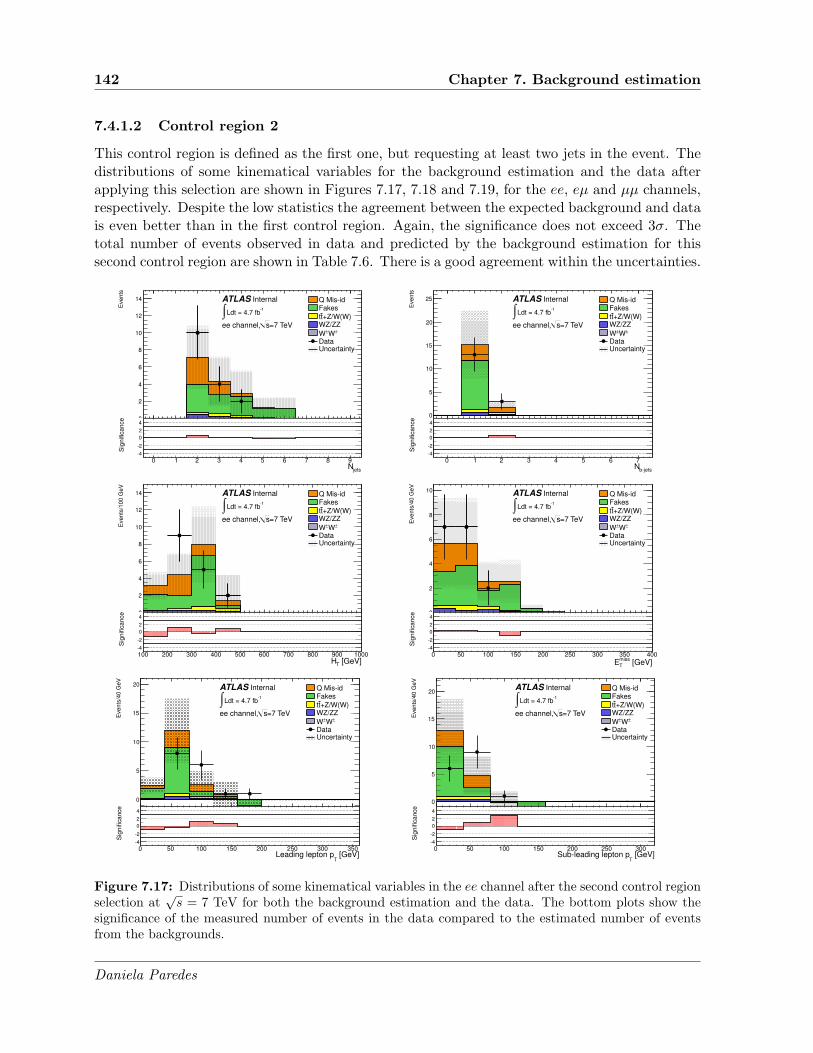
142 Chapter 7. Background estimation
7.4.1.2 Control region 2
This control region is defined as the first one, but requesting at least two jets in the event. Thedistributions of some kinematical variables for the background estimation and the data afterapplying this selection are shown in Figures 7.17, 7.18 and 7.19, for the ee, eµ and µµ channels,respectively. Despite the low statistics the agreement between the expected background and datais even better than in the first control region. Again, the significance does not exceed 3σ. Thetotal number of events observed in data and predicted by the background estimation for thissecond control region are shown in Table 7.6. There is a good agreement within the uncertainties.
Eve
nts
0
2
4
6
8
10
12
14 Q Mis-idFakes
+Z/W(W)ttWZ/ZZ
±W±WDataUncertainty
=7 TeVsee channel,
InternalATLAS
-1Ldt = 4.7 fb∫
jetsN0 1 2 3 4 5 6 7 8 9
Sig
nific
an
ce
-4
-2
0
2
4
Eve
nts
0
5
10
15
20
25 Q Mis-idFakes
+Z/W(W)ttWZ/ZZ
±W±WDataUncertainty
=7 TeVsee channel,
InternalATLAS
-1Ldt = 4.7 fb∫
b-jetsN0 1 2 3 4 5 6 7
Sig
nific
an
ce
-4
-2
0
2
4
Eve
nts
/10
0 G
eV
0
2
4
6
8
10
12
14 Q Mis-idFakes
+Z/W(W)ttWZ/ZZ
±W±WDataUncertainty
=7 TeVsee channel,
InternalATLAS
-1Ldt = 4.7 fb∫
[GeV]TH100 200 300 400 500 600 700 800 900 1000
Sig
nific
an
ce
-4
-2
0
2
4
Eve
nts
/40
Ge
V
0
2
4
6
8
10Q Mis-idFakes
+Z/W(W)ttWZ/ZZ
±W±WDataUncertainty
=7 TeVsee channel,
InternalATLAS
-1Ldt = 4.7 fb∫
[GeV]miss
TE0 50 100 150 200 250 300 350 400
Sig
nific
an
ce
-4
-2
0
2
4
Eve
nts
/40
Ge
V
0
5
10
15
20Q Mis-idFakes
+Z/W(W)ttWZ/ZZ
±W±WDataUncertainty
=7 TeVsee channel,
InternalATLAS
-1Ldt = 4.7 fb∫
[GeV]T
Leading lepton p0 50 100 150 200 250 300 350
Sig
nific
an
ce
-4
-2
0
2
4
Eve
nts
/40
Ge
V
0
5
10
15
20Q Mis-idFakes
+Z/W(W)ttWZ/ZZ
±W±WDataUncertainty
=7 TeVsee channel,
InternalATLAS
-1Ldt = 4.7 fb∫
[GeV]T
Sub-leading lepton p0 50 100 150 200 250 300
Sig
nific
an
ce
-4
-2
0
2
4
Figure 7.17: Distributions of some kinematical variables in the ee channel after the second control regionselection at
√s = 7 TeV for both the background estimation and the data. The bottom plots show the
significance of the measured number of events in the data compared to the estimated number of eventsfrom the backgrounds.
Daniela Paredes

7.4. Background validation 143
Events
0
5
10
15
20
25
30
35
Q Mis-idFakes
+Z/W(W)ttWZ/ZZ
±W±WDataUncertainty
=7 TeVs channel, µe
InternalATLAS
-1Ldt = 4.7 fb∫
jetsN0 1 2 3 4 5 6 7 8 9
Sig
nific
ance
-4
-2
0
2
4
Events
0
10
20
30
40
50Q Mis-idFakes
+Z/W(W)ttWZ/ZZ
±W±WDataUncertainty
=7 TeVs channel, µe
InternalATLAS
-1Ldt = 4.7 fb∫
b-jetsN0 1 2 3 4 5 6 7
Sig
nific
ance
-4
-2
0
2
4
Events
/100 G
eV
0
5
10
15
20
25
30
35 Q Mis-idFakes
+Z/W(W)ttWZ/ZZ
±W±WDataUncertainty
=7 TeVs channel, µe
InternalATLAS
-1Ldt = 4.7 fb∫
[GeV]TH100 200 300 400 500 600 700 800 900 1000
Sig
nific
ance
-4
-2
0
2
4
Events
/40 G
eV
0
5
10
15
20
25
30Q Mis-idFakes
+Z/W(W)ttWZ/ZZ
±W±WDataUncertainty
=7 TeVs channel, µe
InternalATLAS
-1Ldt = 4.7 fb∫
[GeV]miss
TE0 50 100 150 200 250 300 350 400
Sig
nific
ance
-4
-2
0
2
4
Events
/40 G
eV
0
10
20
30
40
Q Mis-idFakes
+Z/W(W)ttWZ/ZZ
±W±WDataUncertainty
=7 TeVs channel, µe
InternalATLAS
-1Ldt = 4.7 fb∫
[GeV]T
Leading lepton p0 50 100 150 200 250 300 350
Sig
nific
ance
-4
-2
0
2
4
Events
/40 G
eV
0
5
10
15
20
25
30
35
40 Q Mis-idFakes
+Z/W(W)ttWZ/ZZ
±W±WDataUncertainty
=7 TeVs channel, µe
InternalATLAS
-1Ldt = 4.7 fb∫
[GeV]T
Sub-leading lepton p0 50 100 150 200 250 300
Sig
nific
ance
-4
-2
0
2
4
Figure 7.18: Distributions of some kinematical variables in the eµ channel after the second controlregion selection at
√s = 7 TeV for both the background estimation and the data. The bottom plots
show the significance of the measured number of events in the data compared to the estimated numberof events from the backgrounds.
Daniela Paredes

144 Chapter 7. Background estimation
Events
0
2
4
6
8
10
12Fakes
+Z/W(W)tt
WZ/ZZ±W±W
Data
Uncertainty
=7 TeVs channel, µµ
InternalATLAS
-1Ldt = 4.7 fb∫
jetsN0 1 2 3 4 5 6 7 8 9
Sig
nific
ance
-4
-2
0
2
4
Events
0
5
10
15
20
25 Fakes
+Z/W(W)tt
WZ/ZZ±W±W
Data
Uncertainty
=7 TeVs channel, µµ
InternalATLAS
-1Ldt = 4.7 fb∫
b-jetsN0 1 2 3 4 5 6 7
Sig
nific
ance
-4
-2
0
2
4
Events
/100 G
eV
0
2
4
6
8
10
12
14
16 Fakes
+Z/W(W)tt
WZ/ZZ±W±W
Data
Uncertainty
=7 TeVs channel, µµ
InternalATLAS
-1Ldt = 4.7 fb∫
[GeV]TH100 200 300 400 500 600 700 800 900 1000
Sig
nific
ance
-4
-2
0
2
4
Events
/40 G
eV
0
2
4
6
8
10
12
14
16Fakes
+Z/W(W)tt
WZ/ZZ±W±W
Data
Uncertainty
=7 TeVs channel, µµ
InternalATLAS
-1Ldt = 4.7 fb∫
[GeV]miss
TE0 50 100 150 200 250 300 350 400
Sig
nific
ance
-4
-2
0
2
4
Events
/40 G
eV
0
2
4
6
8
10
12
14
16
18 Fakes
+Z/W(W)tt
WZ/ZZ±W±W
Data
Uncertainty
=7 TeVs channel, µµ
InternalATLAS
-1Ldt = 4.7 fb∫
[GeV]T
Leading lepton p0 50 100 150 200 250 300 350
Sig
nific
ance
-4
-2
0
2
4
Events
/40 G
eV
0
5
10
15
20
25Fakes
+Z/W(W)tt
WZ/ZZ±W±W
Data
Uncertainty
=7 TeVs channel, µµ
InternalATLAS
-1Ldt = 4.7 fb∫
[GeV]T
Sub-leading lepton p0 50 100 150 200 250 300
Sig
nific
ance
-4
-2
0
2
4
Figure 7.19: Distributions of some kinematical variables in the µµ channel after the second controlregion selection at
√s = 7 TeV for both the background estimation and the data. The bottom plots
show the significance of the measured number of events in the data compared to the estimated numberof events from the backgrounds.
Daniela Paredes

7.4. Background validation 145
ChannelSamples ee eµ µµ
Q Mis-id 5.2± 0.3± 0.6 7.9± 0.3± 1.0 —Fakes 10.0± 5.3± 5.0 34.0± 5.2± 13.6 17.4± 1.8± 5.2
Diboson• WZ/ZZ(+jets) 0.69± 0.23± 0.12 2.15± 0.36± 0.37 2.17± 0.40± 0.44• W±W±jj 0.06± 0.03± 0.03 0.27± 0.06± 0.14 0.15± 0.04± 0.07
tt+W/Z• ttW (+jet) 0.77± 0.04± 0.17 3.34± 0.09± 0.73 2.06± 0.07± 0.45• ttZ(+jet) 0.32± 0.02± 0.12 1.33± 0.05± 0.48 0.88± 0.04± 0.32• ttW+W− 0.008± 0.001± 0.002 0.033± 0.001± 0.010 0.024± 0.001± 0.007
Total 17.0± 5.3± 5.0 49.0± 5.2± 13.7 22.7± 1.8± 5.2
Observed 16 34 18
Signal contamination• tttt C.I. 0.012± 0.003 0.046± 0.005 0.027± 0.004(C/Λ2 = −4π TeV−2)
Table 7.6: Observed number of events and expected number of background events with statistical(first) and systematic (second) uncertainties for the second control region selection at 7 TeV. The signalcontamination in this region is also shown. For the Monte Carlo samples, the systematic uncertaintiesinclude only the production cross section uncertainty.
7.4.1.3 Control region 3
The third control region is defined as the second one, but with the additional requirement ofEmiss
T > 40 GeV. The distributions of some kinematical variables for the background estimationand the data after applying this selection are shown in Figures 7.20, 7.21 and 7.22, for the ee,eµ and µµ channels, respectively. In terms of significance there is a better agreement than inthe previous control regions since it does not exceed 2σ. The total number of events observedin data and predicted by the background estimation for this third control region are shown inTable 7.7. They are compatible within the uncertainties.
7.4.1.4 Control region 4
A last control region is defined, but this time in the high HT region. It requires the followingselection:
• Events must contain at least one same-sign pair of leptons.
• Events must contain at least one b-tagged jet. There is no other requirement on the numberof jets.
• Z veto in ee and µµ channels.
• HT > 400 GeV and EmissT < 40 GeV.
In this control region, the statistics here is very low as to show distributions. The totalnumber of events observed in data and predicted by the background estimation for this fourthcontrol region are shown in Table 7.8. They are compatible within the uncertainties.
Daniela Paredes

146 Chapter 7. Background estimation
Events
0
1
2
3
4
5
6
7
8Q Mis-idFakes
+Z/W(W)ttWZ/ZZ
±W±WDataUncertainty
=7 TeVsee channel,
InternalATLAS
-1Ldt = 4.7 fb∫
jetsN0 1 2 3 4 5 6 7 8 9
Sig
nific
ance
-4
-2
0
2
4
Events
0
2
4
6
8
10
12
14
16
18 Q Mis-idFakes
+Z/W(W)ttWZ/ZZ
±W±WDataUncertainty
=7 TeVsee channel,
InternalATLAS
-1Ldt = 4.7 fb∫
b-jetsN0 1 2 3 4 5 6 7
Sig
nific
ance
-4
-2
0
2
4
Events
/100 G
eV
0
1
2
3
4
5
6
7Q Mis-idFakes
+Z/W(W)ttWZ/ZZ
±W±WDataUncertainty
=7 TeVsee channel,
InternalATLAS
-1Ldt = 4.7 fb∫
[GeV]TH100 200 300 400 500 600 700 800 900 1000
Sig
nific
ance
-4
-2
0
2
4
Events
/40 G
eV
0
1
2
3
4
5
6
7
8
9 Q Mis-idFakes
+Z/W(W)ttWZ/ZZ
±W±WDataUncertainty
=7 TeVsee channel,
InternalATLAS
-1Ldt = 4.7 fb∫
[GeV]miss
TE0 50 100 150 200 250 300 350 400
Sig
nific
ance
-4
-2
0
2
4
Events
/40 G
eV
0
2
4
6
8
10
Q Mis-idFakes
+Z/W(W)ttWZ/ZZ
±W±WDataUncertainty
=7 TeVsee channel,
InternalATLAS
-1Ldt = 4.7 fb∫
[GeV]T
Leading lepton p0 50 100 150 200 250 300 350
Sig
nific
ance
-4
-2
0
2
4
Events
/40 G
eV
0
2
4
6
8
10
12Q Mis-idFakes
+Z/W(W)ttWZ/ZZ
±W±WDataUncertainty
=7 TeVsee channel,
InternalATLAS
-1Ldt = 4.7 fb∫
[GeV]T
Sub-leading lepton p0 50 100 150 200 250 300
Sig
nific
ance
-4
-2
0
2
4
Figure 7.20: Distributions of some kinematical variables in the ee channel after the third control regionselection at
√s = 7 TeV for both the background estimation and the data. The bottom plots show the
significance of the measured number of events in the data compared to the estimated number of eventsfrom the backgrounds
Daniela Paredes
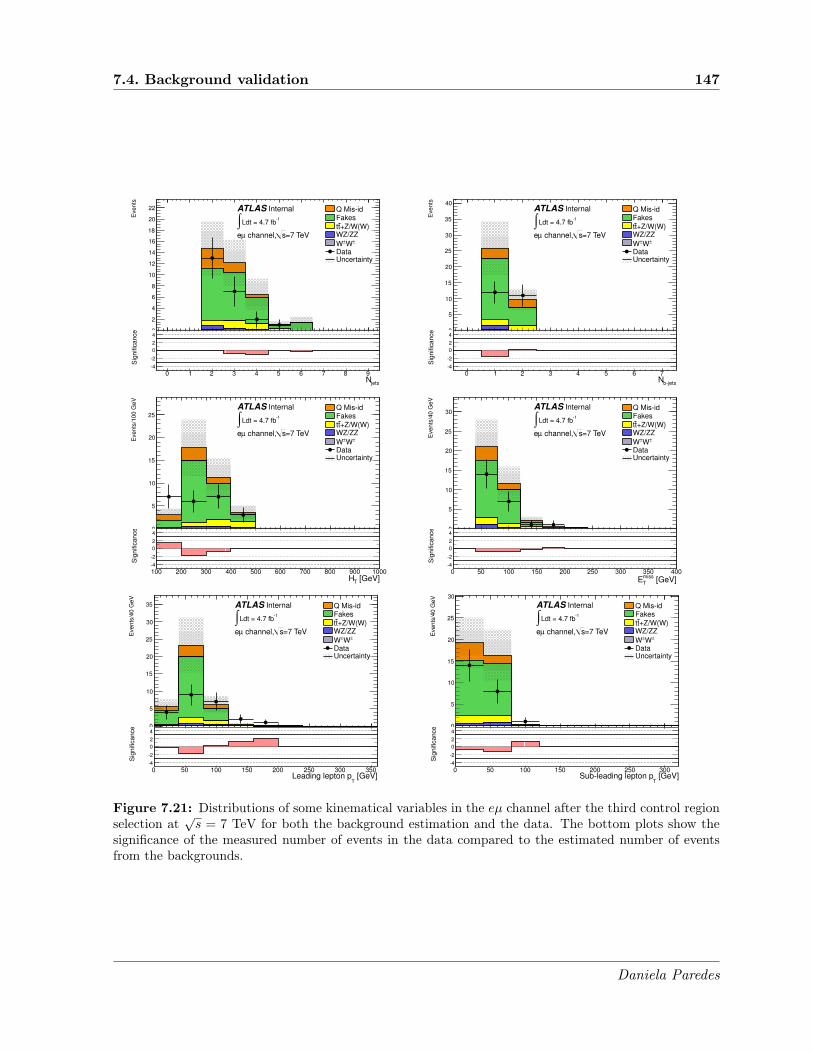
7.4. Background validation 147
Events
0
2
4
6
8
10
12
14
16
18
20
22 Q Mis-idFakes
+Z/W(W)ttWZ/ZZ
±W±WDataUncertainty
=7 TeVs channel, µe
InternalATLAS
-1Ldt = 4.7 fb∫
jetsN0 1 2 3 4 5 6 7 8 9
Sig
nific
ance
-4
-2
0
2
4
Events
0
5
10
15
20
25
30
35
40Q Mis-idFakes
+Z/W(W)ttWZ/ZZ
±W±WDataUncertainty
=7 TeVs channel, µe
InternalATLAS
-1Ldt = 4.7 fb∫
b-jetsN0 1 2 3 4 5 6 7
Sig
nific
ance
-4
-2
0
2
4
Events
/100 G
eV
0
5
10
15
20
25Q Mis-idFakes
+Z/W(W)ttWZ/ZZ
±W±WDataUncertainty
=7 TeVs channel, µe
InternalATLAS
-1Ldt = 4.7 fb∫
[GeV]TH100 200 300 400 500 600 700 800 900 1000
Sig
nific
ance
-4
-2
0
2
4
Events
/40 G
eV
0
5
10
15
20
25
30Q Mis-idFakes
+Z/W(W)ttWZ/ZZ
±W±WDataUncertainty
=7 TeVs channel, µe
InternalATLAS
-1Ldt = 4.7 fb∫
[GeV]miss
TE0 50 100 150 200 250 300 350 400
Sig
nific
ance
-4
-2
0
2
4
Events
/40 G
eV
0
5
10
15
20
25
30
35 Q Mis-idFakes
+Z/W(W)ttWZ/ZZ
±W±WDataUncertainty
=7 TeVs channel, µe
InternalATLAS
-1Ldt = 4.7 fb∫
[GeV]T
Leading lepton p0 50 100 150 200 250 300 350
Sig
nific
ance
-4
-2
0
2
4
Events
/40 G
eV
0
5
10
15
20
25
30
Q Mis-idFakes
+Z/W(W)ttWZ/ZZ
±W±WDataUncertainty
=7 TeVs channel, µe
InternalATLAS
-1Ldt = 4.7 fb∫
[GeV]T
Sub-leading lepton p0 50 100 150 200 250 300
Sig
nific
ance
-4
-2
0
2
4
Figure 7.21: Distributions of some kinematical variables in the eµ channel after the third control regionselection at
√s = 7 TeV for both the background estimation and the data. The bottom plots show the
significance of the measured number of events in the data compared to the estimated number of eventsfrom the backgrounds.
Daniela Paredes

148 Chapter 7. Background estimation
Events
0
2
4
6
8
10Fakes
+Z/W(W)tt
WZ/ZZ±W±W
Data
Uncertainty
=7 TeVs channel, µµ
InternalATLAS
-1Ldt = 4.7 fb∫
jetsN0 1 2 3 4 5 6 7 8 9
Sig
nific
ance
-4
-2
0
2
4
Events
0
2
4
6
8
10
12
14
16
18 Fakes
+Z/W(W)tt
WZ/ZZ±W±W
Data
Uncertainty
=7 TeVs channel, µµ
InternalATLAS
-1Ldt = 4.7 fb∫
b-jetsN0 1 2 3 4 5 6 7
Sig
nific
ance
-4
-2
0
2
4
Events
/100 G
eV
0
1
2
3
4
5
6
7
8
9 Fakes
+Z/W(W)tt
WZ/ZZ±W±W
Data
Uncertainty
=7 TeVs channel, µµ
InternalATLAS
-1Ldt = 4.7 fb∫
[GeV]TH100 200 300 400 500 600 700 800 900 1000
Sig
nific
ance
-4
-2
0
2
4
Events
/40 G
eV
0
2
4
6
8
10
12
14
16Fakes
+Z/W(W)tt
WZ/ZZ±W±W
Data
Uncertainty
=7 TeVs channel, µµ
InternalATLAS
-1Ldt = 4.7 fb∫
[GeV]miss
TE0 50 100 150 200 250 300 350 400
Sig
nific
ance
-4
-2
0
2
4
Events
/40 G
eV
0
2
4
6
8
10
12 Fakes
+Z/W(W)tt
WZ/ZZ±W±W
Data
Uncertainty
=7 TeVs channel, µµ
InternalATLAS
-1Ldt = 4.7 fb∫
[GeV]T
Leading lepton p0 50 100 150 200 250 300 350
Sig
nific
ance
-4
-2
0
2
4
Events
/40 G
eV
0
5
10
15
20Fakes
+Z/W(W)tt
WZ/ZZ±W±W
Data
Uncertainty
=7 TeVs channel, µµ
InternalATLAS
-1Ldt = 4.7 fb∫
[GeV]T
Sub-leading lepton p0 50 100 150 200 250 300
Sig
nific
ance
-4
-2
0
2
4
Figure 7.22: Distributions of some kinematical variables in the µµ channel after the third control regionselection at
√s = 7 TeV for both the background estimation and the data. The bottom plots show the
significance of the measured number of events in the data compared to the estimated number of eventsfrom the backgrounds.
Daniela Paredes

7.4. Background validation 149
ChannelSamples ee eµ µµ
Q Mis-id 2.88± 0.17± 0.35 6.01± 0.24± 0.72 —Fakes 7.10± 3.99± 3.55 24.9± 4.6± 9.9 12.2± 1.4± 3.6
Diboson• WZ/ZZ(+jets) 0.40± 0.21± 0.08 1.21± 0.29± 0.23 1.40± 0.33± 0.28• W±W±jj 0.05± 0.03± 0.03 0.19± 0.05± 0.09 0.13± 0.04± 0.07
tt+W/Z• ttW (+jet) 0.61± 0.04± 0.14 2.72± 0.08± 0.59 1.66± 0.06± 0.36• ttZ(+jet) 0.23± 0.02± 0.09 1.03± 0.04± 0.37 0.66± 0.03± 0.24• ttW+W− 0.006± 0.001± 0.002 0.028± 0.001± 0.008 0.021± 0.001± 0.006
Total 11.3± 4.0± 3.6 36.1± 4.6± 10.0 16.1± 1.4± 3.6
Observed 9 23 13
Signal contamination• tttt C.I. 0.010± 0.002 0.039± 0.005 0.022± 0.004(C/Λ2 = −4π TeV−2)
Table 7.7: Observed number of events and expected number of background events with statistical(first) and systematic (second) uncertainties for the third control region selection at 7 TeV. The signalcontamination in this region is also shown. For the Monte Carlo samples, the systematic uncertaintiesinclude only the production cross section uncertainty.
ChannelSamples ee eµ µµ
Q Mis-id 0.33± 0.08± 0.04 0.17± 0.04± 0.02 —Fakes 2.28± 3.21± 1.14 1.19± 1.19± 0.48 0.71± 0.32± 0.21
Diboson• WZ/ZZ(+jets) 0.20± 0.21± 0.05 0.92± 0.33± 0.15 0.25± 0.19± 0.06• W±W±jj 0± 0.01 0.014± 0.014± 0.007 0.03± 0.02± 0.01
tt+W/Z• ttW (+jet) 0.10± 0.02± 0.02 0.31± 0.03± 0.07 0.18± 0.02± 0.04• ttZ(+jet) 0.10± 0.01± 0.03 0.33± 0.02± 0.12 0.22± 0.02± 0.08• ttW+W− 0.0022± 0.0004± 0.0007 0.0064± 0.0007± 0.0019 0.0046± 0.0005± 0.0014
Total 3.01± 3.22± 1.14 2.94± 1.24± 0.52 1.39± 0.37± 0.24
Observed 1 4 0
Signal contamination• tttt C.I. 0.018± 0.004 0.058± 0.006 0.041± 0.005(C/Λ2 = −4π TeV−2)
Table 7.8: Observed number of events and expected number of background events with statistical(first) and systematic (second) uncertainties for the fourth control region selection at 7 TeV. The signalcontamination in this region is also shown. For the Monte Carlo samples, the systematic uncertaintiesinclude only the production cross section uncertainty.
Daniela Paredes

150 Chapter 7. Background estimation
7.4.2 Control regions at√s = 8 TeV
Three different control regions have been defined in the analysis at 8 TeV. They allow to controlthe Emiss
T , HT, and both distributions at the same time. They are defined as explained below.
7.4.2.1 Control region 1
This control region has been defined similarly as the EmissT control region as for the analysis at
7 TeV, but it restricts a little more the low HT region. It requires the following event selection:
• Events must contain exactly one same-sign pair of leptons.
• Events must contain at least two jets with one b-tagged jet
• Z veto in the ee and µµ channels.
• HT ∈ [100, 400] GeV.
The distributions of some kinematical variables for the background estimation and thedata after applying this selection are shown in Figures 7.23, 7.24 and 7.25, for the ee, eµ andµµ channels, respectively. The total number of events observed in data and predicted by thebackground estimation for this first control region are shown in Table 7.9. A good agreementwithin uncertainties is observed.
ChannelSamples ee eµ µµ
Q Mis-id 25.66± 0.68± 6.64 30.24± 0.64± 7.92 —Fakes 38.7± 3.67± 11.6 73.1± 5.3± 21.9 33.4± 8.5± 10.0
Diboson• WZ/ZZ(+jets) 3.85± 0.68± 1.31 10.92± 1.22± 3.71 5.10± 0.82± 1.73• W±W±jj 0.43± 0.16± 0.22 1.18± 0.26± 0.59 0.75± 0.20± 0.38
tt+W/Z• ttW (+jet(s)) 1.65± 0.10± 0.50 6.6± 0.2± 2.0 4.31± 0.17± 1.29• ttZ(+jet(s)) 0.48± 0.05± 0.14 1.50± 0.09± 0.45 0.79± 0.06± 0.24• ttW+W− 0.014± 0.002 0.050± 0.004 0.029± 0.003
Total 71± 5± 13 124± 8± 24 44± 11± 10
Observed 64 97 38
Signal contamination• tttt C.I. 0.009± 0.005 0.06± 0.02 0.02± 0.01(C/Λ2 = −4π TeV−2)
Table 7.9: Observed number of events and expected number of background events with statistical(first) and systematic (second) uncertainties for the Emiss
T control region selection at 8 TeV. The signalcontamination in this region is also shown. For the Monte Carlo samples, the systematic uncertaintiesinclude only the production cross section uncertainty
Daniela Paredes

7.4. Background validation 151
En
trie
s
0
10
20
30
40
50
Data
Q Mis-id
Fakes
+Z/W(W)tt
WZ/ZZ
±W±W
=8 TeVsee channel,
ATLASPreliminary
-1Ldt = 14.3 fb∫
jetsN0 2 4 6 8 10 12 14
Sig
nific
an
ce
-3
0
3
En
trie
s
0
10
20
30
40
50
60
70
Data
Q Mis-id
Fakes
+Z/W(W)tt
WZ/ZZ
±W±W
=8 TeVsee channel,
ATLASPreliminary
-1Ldt = 14.3 fb∫
b-jetsN0 1 2 3 4 5 6 7
Sig
nific
an
ce
-3
0
3
En
trie
s
0
5
10
15
20
25
30
35
40
Data
Q Mis-id
Fakes
+Z/W(W)tt
WZ/ZZ
±W±W
=8 TeVsee channel,
ATLASPreliminary
-1Ldt = 14.3 fb∫
[GeV]TH0 200 400 600 800 1000 1200 1400 1600 1800 2000
Sig
nific
an
ce
-3
0
3
En
trie
s
0
5
10
15
20
25
30
35
40
45
Data
Q Mis-id
Fakes
+Z/W(W)tt
WZ/ZZ
±W±W
=8 TeVsee channel,
ATLASPreliminary
-1Ldt = 14.3 fb∫
[GeV]miss
TE0 100 200 300 400 500 600 700 800
Sig
nific
an
ce
-3
0
3
En
trie
s
0
10
20
30
40
50
Data
Q Mis-id
Fakes
+Z/W(W)tt
WZ/ZZ
±W±W
=8 TeVsee channel,
ATLASPreliminary
-1Ldt = 14.3 fb∫
[GeV]T
Leading lepton p0 100 200 300 400 500
Sig
nific
an
ce
-3
0
3
En
trie
s
0
10
20
30
40
50
Data
Q Mis-id
Fakes
+Z/W(W)tt
WZ/ZZ
±W±W
=8 TeVsee channel,
ATLASPreliminary
-1Ldt = 14.3 fb∫
[GeV]T
Sub-leading lepton p0 50 100 150 200 250 300
Sig
nific
an
ce
-3
0
3
Figure 7.23: Distributions of some kinematical variables in the ee channel, after the EmissT control
region selection at 8 TeV, for both the background estimation and the data. The bottom plots show thesignificance of the measured number of events in the data compared to the estimated number of eventsfrom the backgrounds.
Daniela Paredes

152 Chapter 7. Background estimationE
ntr
ies
0
10
20
30
40
50
60
70
Data
Q Mis-id
Fakes
+Z/W(W)tt
WZ/ZZ
±W±W
=8 TeVs channel, µe
ATLASPreliminary
-1Ldt = 14.3 fb∫
jetsN0 2 4 6 8 10 12 14
Sig
nific
an
ce
-3
0
3
En
trie
s
0
20
40
60
80
100
120
Data
Q Mis-id
Fakes
+Z/W(W)tt
WZ/ZZ
±W±W
=8 TeVs channel, µe
ATLASPreliminary
-1Ldt = 14.3 fb∫
b-jetsN0 1 2 3 4 5 6 7
Sig
nific
an
ce
-3
0
3
En
trie
s
0
10
20
30
40
50
60
70
80
Data
Q Mis-id
Fakes
+Z/W(W)tt
WZ/ZZ
±W±W
=8 TeVs channel, µe
ATLASPreliminary
-1Ldt = 14.3 fb∫
[GeV]TH0 200 400 600 800 1000 1200 1400 1600 1800 2000
Sig
nific
an
ce
-3
0
3
En
trie
s
0
10
20
30
40
50
60
Data
Q Mis-id
Fakes
+Z/W(W)tt
WZ/ZZ
±W±W
=8 TeVs channel, µe
ATLASPreliminary
-1Ldt = 14.3 fb∫
[GeV]miss
TE0 100 200 300 400 500 600 700 800
Sig
nific
an
ce
-3
0
3
En
trie
s
0
10
20
30
40
50
60
70
80
90
Data
Q Mis-id
Fakes
+Z/W(W)tt
WZ/ZZ
±W±W
=8 TeVs channel, µe
ATLASPreliminary
-1Ldt = 14.3 fb∫
[GeV]T
Leading lepton p0 100 200 300 400 500
Sig
nific
an
ce
-3
0
3
En
trie
s
0
20
40
60
80
100
Data
Q Mis-id
Fakes
+Z/W(W)tt
WZ/ZZ
±W±W
=8 TeVs channel, µe
ATLASPreliminary
-1Ldt = 14.3 fb∫
[GeV]T
Sub-leading lepton p0 50 100 150 200 250 300
Sig
nific
an
ce
-3
0
3
Figure 7.24: Distributions of some kinematical variables in the eµ channel, after the EmissT control
region selection at 8 TeV, for both the background estimation and the data. The bottom plots show thesignificance of the measured number of events in the data compared to the estimated number of eventsfrom the backgrounds.
Daniela Paredes
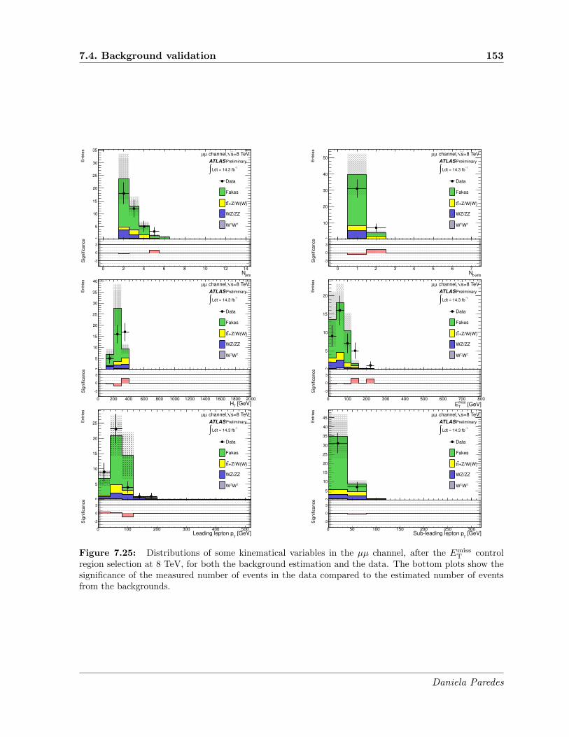
7.4. Background validation 153
En
trie
s
0
5
10
15
20
25
30
35
Data
Fakes
+Z/W(W)tt
WZ/ZZ
±W±W
=8 TeVs channel, µµ
ATLASPreliminary
-1Ldt = 14.3 fb∫
jetsN0 2 4 6 8 10 12 14
Sig
nific
an
ce
-3
0
3
En
trie
s
0
10
20
30
40
50
Data
Fakes
+Z/W(W)tt
WZ/ZZ
±W±W
=8 TeVs channel, µµ
ATLASPreliminary
-1Ldt = 14.3 fb∫
b-jetsN0 1 2 3 4 5 6 7
Sig
nific
an
ce
-3
0
3
En
trie
s
0
5
10
15
20
25
30
35
40
Data
Fakes
+Z/W(W)tt
WZ/ZZ
±W±W
=8 TeVs channel, µµ
ATLASPreliminary
-1Ldt = 14.3 fb∫
[GeV]TH0 200 400 600 800 1000 1200 1400 1600 1800 2000
Sig
nific
an
ce
-3
0
3
En
trie
s
0
5
10
15
20
Data
Fakes
+Z/W(W)tt
WZ/ZZ
±W±W
=8 TeVs channel, µµ
ATLASPreliminary
-1Ldt = 14.3 fb∫
[GeV]miss
TE0 100 200 300 400 500 600 700 800
Sig
nific
an
ce
-3
0
3
En
trie
s
0
5
10
15
20
25
Data
Fakes
+Z/W(W)tt
WZ/ZZ
±W±W
=8 TeVs channel, µµ
ATLASPreliminary
-1Ldt = 14.3 fb∫
[GeV]T
Leading lepton p0 100 200 300 400 500
Sig
nific
an
ce
-3
0
3
En
trie
s
0
5
10
15
20
25
30
35
40
45
Data
Fakes
+Z/W(W)tt
WZ/ZZ
±W±W
=8 TeVs channel, µµ
ATLASPreliminary
-1Ldt = 14.3 fb∫
[GeV]T
Sub-leading lepton p0 50 100 150 200 250 300
Sig
nific
an
ce
-3
0
3
Figure 7.25: Distributions of some kinematical variables in the µµ channel, after the EmissT control
region selection at 8 TeV, for both the background estimation and the data. The bottom plots show thesignificance of the measured number of events in the data compared to the estimated number of eventsfrom the backgrounds.
Daniela Paredes

154 Chapter 7. Background estimation
7.4.2.2 Control region 2
The second control region is called “HT control region”. The event selection is the following:
• Events must contain exactly one same-sign pair of leptons.
• Events must contain at least two jets with one b-tagged jet.
• Z veto in the ee or µµ channel.
• EmissT < 40 GeV.
• HT > 100 GeV.
Comparing to the event preselection, the cut on HT has been removed, and the one on EmissT
has been reverted. Therefore, this region allows to control the HT distribution, but in a lowEmiss
T region. The distributions of some kinematic variables for the background estimation andthe data after applying this HT control region selection are shown in Figures 7.26, 7.27 and 7.28for the ee, eµ and µµ channels, respectively. The total number of events observed in data andpredicted by the background estimation for this second control region are shown in Table 7.10.Again, the agreement between the measured number of events and the predicted one from thebackground estimation is good.
ChannelSamples ee eµ µµ
Q Mis-id 13.29± 0.52± 3.54 9.27± 0.37± 2.47 —Fakes 24.27± 3.33± 7.28 34.0± 3.9± 10.2 11.69± 6.86± 3.51
Diboson• WZ/ZZ(+jets) 2.60± 0.56± 0.88 7.09± 0.97± 2.41 2.40± 0.59± 0.82• W±W±jj 0.09± 0.06± 0.05 0.70± 0.20± 0.35 0.38± 0.14± 0.19
tt+W/Z• ttW (+jet(s)) 0.60± 0.06± 0.18 2.52± 0.12± 0.76 1.61± 0.10± 0.48• ttZ(+jet(s)) 0.38± 0.04± 0.11 0.96± 0.06± 0.29 0.54± 0.05± 0.16• ttW+W− 0.007± 0.001 0.034± 0.003 0.021± 0.003
Total 41± 5± 8 55± 6± 11 17± 9± 4
Observed 35 39 10
Signal contamination• tttt C.I. 0.10± 0.03 0.34± 0.05 0.41± 0.05(C/Λ2 = −4π TeV−2)
Table 7.10: Observed number of events and expected number of background events with statistical(first) and systematic (second) uncertainties for the HT control region selection at 8 TeV. The signalcontamination in this region is also shown. For the Monte Carlo samples, the systematic uncertaintiesinclude only the production cross section uncertainty.
Daniela Paredes

7.4. Background validation 155
En
trie
s
0
5
10
15
20
25
Data
Q Mis-id
Fakes
+Z/W(W)tt
WZ/ZZ
±W±W
=8 TeVsee channel,
ATLAS Internal
-1Ldt = 14.3 fb∫
jetsN0 2 4 6 8 10 12 14
Sig
nific
an
ce
-5-4-3-2-1012345
En
trie
s
0
5
10
15
20
25
30
35
40
Data
Q Mis-id
Fakes
+Z/W(W)tt
WZ/ZZ
±W±W
=8 TeVsee channel,
ATLAS Internal
-1Ldt = 14.3 fb∫
b-jetsN0 1 2 3 4 5 6 7
Sig
nific
an
ce
-5-4-3-2-1012345
En
trie
s
0
5
10
15
20
Data
Q Mis-id
Fakes
+Z/W(W)tt
WZ/ZZ
±W±W
=8 TeVsee channel,
ATLAS Internal
-1Ldt = 14.3 fb∫
[GeV]TH0 200 400 600 800 1000 1200 1400 1600 1800 2000
Sig
nific
an
ce
-5-4-3-2-1012345
En
trie
s
0
10
20
30
40
50
Data
Q Mis-id
Fakes
+Z/W(W)tt
WZ/ZZ
±W±W
=8 TeVsee channel,
ATLAS Internal
-1Ldt = 14.3 fb∫
[GeV]miss
TE0 100 200 300 400 500 600 700 800
Sig
nific
an
ce
-5-4-3-2-1012345
En
trie
s
0
5
10
15
20
25
30
Data
Q Mis-id
Fakes
+Z/W(W)tt
WZ/ZZ
±W±W
=8 TeVsee channel,
ATLAS Internal
-1Ldt = 14.3 fb∫
[GeV]T
Leading lepton p0 100 200 300 400 500
Sig
nific
an
ce
-5-4-3-2-1012345
En
trie
s
0
5
10
15
20
25
30
Data
Q Mis-id
Fakes
+Z/W(W)tt
WZ/ZZ
±W±W
=8 TeVsee channel,
ATLAS Internal
-1Ldt = 14.3 fb∫
[GeV]T
Sub-leading lepton p0 50 100 150 200 250 300
Sig
nific
an
ce
-5-4-3-2-1012345
Figure 7.26: Distributions of some kinematic variables in the ee channel, after the HT control regionselection at 8 TeV, for both the background estimation and the data. The bottom plots show the signif-icance of the measured number of events in the data compared to the estimated number of events fromthe backgrounds.
Daniela Paredes

156 Chapter 7. Background estimationE
ntr
ies
0
5
10
15
20
25
30
Data
Q Mis-id
Fakes
+Z/W(W)tt
WZ/ZZ
±W±W
=8 TeVs channel, µe
ATLAS Internal
-1Ldt = 14.3 fb∫
jetsN0 2 4 6 8 10 12 14
Sig
nific
an
ce
-5-4-3-2-1012345
En
trie
s
0
10
20
30
40
50
Data
Q Mis-id
Fakes
+Z/W(W)tt
WZ/ZZ
±W±W
=8 TeVs channel, µe
ATLAS Internal
-1Ldt = 14.3 fb∫
b-jetsN0 1 2 3 4 5 6 7
Sig
nific
an
ce
-5-4-3-2-1012345
En
trie
s
0
5
10
15
20
25
30
Data
Q Mis-id
Fakes
+Z/W(W)tt
WZ/ZZ
±W±W
=8 TeVs channel, µe
ATLAS Internal
-1Ldt = 14.3 fb∫
[GeV]TH0 200 400 600 800 1000 1200 1400 1600 1800 2000
Sig
nific
an
ce
-5-4-3-2-1012345
En
trie
s
0
10
20
30
40
50
60
Data
Q Mis-id
Fakes
+Z/W(W)tt
WZ/ZZ
±W±W
=8 TeVs channel, µe
ATLAS Internal
-1Ldt = 14.3 fb∫
[GeV]miss
TE0 100 200 300 400 500 600 700 800
Sig
nific
an
ce
-5-4-3-2-1012345
En
trie
s
0
5
10
15
20
25
30
35
Data
Q Mis-id
Fakes
+Z/W(W)tt
WZ/ZZ
±W±W
=8 TeVs channel, µe
ATLAS Internal
-1Ldt = 14.3 fb∫
[GeV]T
Leading lepton p0 100 200 300 400 500
Sig
nific
an
ce
-5-4-3-2-1012345
En
trie
s
0
5
10
15
20
25
30
35
40
45
Data
Q Mis-id
Fakes
+Z/W(W)tt
WZ/ZZ
±W±W
=8 TeVs channel, µe
ATLAS Internal
-1Ldt = 14.3 fb∫
[GeV]T
Sub-leading lepton p0 50 100 150 200 250 300
Sig
nific
an
ce
-5-4-3-2-1012345
Figure 7.27: Distributions of some kinematic variables in the eµ channel, after the HT control regionselection at 8 TeV, for both the background estimation and the data. The bottom plots show the signif-icance of the measured number of events in the data compared to the estimated number of events fromthe backgrounds.
Daniela Paredes

7.4. Background validation 157
En
trie
s
0
2
4
6
8
10
12
14
16
Data
Fakes
+Z/W(W)tt
WZ/ZZ
±W±W
=8 TeVs channel, µµ
ATLAS Internal
-1Ldt = 14.3 fb∫
jetsN0 2 4 6 8 10 12 14
Sig
nific
an
ce
-5-4-3-2-1012345
En
trie
s
0
2
4
6
8
10
12
14
16
18
20
22
Data
Fakes
+Z/W(W)tt
WZ/ZZ
±W±W
=8 TeVs channel, µµ
ATLAS Internal
-1Ldt = 14.3 fb∫
b-jetsN0 1 2 3 4 5 6 7
Sig
nific
an
ce
-5-4-3-2-1012345
En
trie
s
0
2
4
6
8
10
12
14
16
18
Data
Fakes
+Z/W(W)tt
WZ/ZZ
±W±W
=8 TeVs channel, µµ
ATLAS Internal
-1Ldt = 14.3 fb∫
[GeV]TH0 200 400 600 800 1000 1200 1400 1600 1800 2000
Sig
nific
an
ce
-5-4-3-2-1012345
En
trie
s
0
5
10
15
20
25
Data
Fakes
+Z/W(W)tt
WZ/ZZ
±W±W
=8 TeVs channel, µµ
ATLAS Internal
-1Ldt = 14.3 fb∫
[GeV]miss
TE0 100 200 300 400 500 600 700 800
Sig
nific
an
ce
-5-4-3-2-1012345
En
trie
s
0
2
4
6
8
10
12
14
16
Data
Fakes
+Z/W(W)tt
WZ/ZZ
±W±W
=8 TeVs channel, µµ
ATLAS Internal
-1Ldt = 14.3 fb∫
[GeV]T
Leading lepton p0 100 200 300 400 500
Sig
nific
an
ce
-5-4-3-2-1012345
En
trie
s
0
2
4
6
8
10
12
14
16
18
20
Data
Fakes
+Z/W(W)tt
WZ/ZZ
±W±W
=8 TeVs channel, µµ
ATLAS Internal
-1Ldt = 14.3 fb∫
[GeV]T
Sub-leading lepton p0 50 100 150 200 250 300
Sig
nific
an
ce
-5-4-3-2-1012345
Figure 7.28: Distributions of some kinematic variables in the µµ channel, after the HT control regionselection at 8 TeV, for both the background estimation and the data. The bottom plots show the signif-icance of the measured number of events in the data compared to the estimated number of events fromthe backgrounds.
Daniela Paredes

158 Chapter 7. Background estimation
7.4.2.3 Control region 3
The third control region is called “zero-b-tag control region”. The event selection is the following:
• Events must contain exactly one same-sign pair of leptons.
• Events must contain at least two jets but zero b-tagged jet.
• Z veto in the ee or µµ channel.
• HT > 100 GeV.
Comparing to the event preselection, the cuts on HT and EmissT have been removed, and
no b-jets are requested. Therefore, this region allows to control the HT and EmissT distributions,
but in a region without b-jets. The distributions of some kinematic variables for the backgroundestimation and the data after applying this zero-b-tag control region selection are shown inFigures 7.29, 7.30 and 7.31 for the ee, eµ and µµ channels, respectively. The total number ofevents observed in data and predicted by the background estimation for this third control regionare shown in Table 7.11. Despite the differences in the ee channel, the significance is less than 3σ.
ChannelSamples ee eµ µµ
Q Mis-id 99.07± 1.55± 26.29 11.95± 0.44± 3.23 —Fakes 80.22± 8.01± 24.1 80.72± 6.07± 24.2 21.34± 3.97± 6.40
Diboson• WZ/ZZ + jets 40.46± 2.05± 13.76 89.93± 3.03± 30.47 36.70± 1.97± 12.48• W±W±jj 6.03± 0.54± 3.02 21.95± 1.04± 10.98 12.03± 0.76± 6.02
tt+W/Z• ttW (+jet(s)) 0.89± 0.08± 0.27 2.85± 0.14± 0.86 2.01± 0.12± 0.60• ttZ(+jet(s)) 0.29± 0.04± 0.09 0.99± 0.07± 0.30 0.50± 0.06± 0.15• ttW+W− 0.021± 0.003 0.053± 0.004 0.039± 0.004
Total 227± 12± 38 208± 11± 41 73± 8± 15
Observed 281 205 80
Signal contamination• tttt C.I. 0.06± 0.02 0.17± 0.04 0.12± 0.03(C/Λ2 = −4π TeV−2)
Table 7.11: Observed number of events and expected number of background events with statistical (first)and systematic (second) uncertainties for the zero-b-tag control region selection at 8 TeV. The signalcontamination in this region is also shown. For the Monte Carlo samples, the systematic uncertaintiesinclude only the production cross section uncertainty.
Daniela Paredes

7.4. Background validation 159
En
trie
s
0
20
40
60
80
100
120
140
160
180
200
220
Data
Q Mis-id
Fakes
+Z/W(W)tt
WZ/ZZ
±W±W
=8 TeVsee channel,
ATLAS Internal
-1Ldt = 14.3 fb∫
jetsN0 2 4 6 8 10 12 14
Sig
nific
an
ce
-5-4-3-2-1012345
En
trie
s
0
50
100
150
200
250
300
Data
Q Mis-id
Fakes
+Z/W(W)tt
WZ/ZZ
±W±W
=8 TeVsee channel,
ATLAS Internal
-1Ldt = 14.3 fb∫
b-jetsN0 1 2 3 4 5 6 7
Sig
nific
an
ce
-5-4-3-2-1012345
En
trie
s
0
20
40
60
80
100
Data
Q Mis-id
Fakes
+Z/W(W)tt
WZ/ZZ
±W±W
=8 TeVsee channel,
ATLAS Internal
-1Ldt = 14.3 fb∫
[GeV]TH0 200 400 600 800 1000 1200 1400 1600 1800 2000
Sig
nific
an
ce
-5-4-3-2-1012345
En
trie
s
0
50
100
150
200
Data
Q Mis-id
Fakes
+Z/W(W)tt
WZ/ZZ
±W±W
=8 TeVsee channel,
ATLAS Internal
-1Ldt = 14.3 fb∫
[GeV]miss
TE0 100 200 300 400 500 600 700 800
Sig
nific
an
ce
-5-4-3-2-1012345
En
trie
s
0
20
40
60
80
100
120
140
Data
Q Mis-id
Fakes
+Z/W(W)tt
WZ/ZZ
±W±W
=8 TeVsee channel,
ATLAS Internal
-1Ldt = 14.3 fb∫
[GeV]T
Leading lepton p0 100 200 300 400 500
Sig
nific
an
ce
-5-4-3-2-1012345
En
trie
s
0
20
40
60
80
100
120
140
160
Data
Q Mis-id
Fakes
+Z/W(W)tt
WZ/ZZ
±W±W
=8 TeVsee channel,
ATLAS Internal
-1Ldt = 14.3 fb∫
[GeV]T
Sub-leading lepton p0 50 100 150 200 250 300
Sig
nific
an
ce
-5-4-3-2-1012345
Figure 7.29: Distributions of some kinematic variables in the ee channel, after the zero-b-tag controlregion selection at 8 TeV, for both the background estimation and the data. The bottom plots show thesignificance of the measured number of events in the data compared to the estimated number of eventsfrom the backgrounds.
Daniela Paredes

160 Chapter 7. Background estimationE
ntr
ies
0
20
40
60
80
100
120
140
160
Data
Q Mis-id
Fakes
+Z/W(W)tt
WZ/ZZ
±W±W
=8 TeVs channel, µe
ATLAS Internal
-1Ldt = 14.3 fb∫
jetsN0 2 4 6 8 10 12 14
Sig
nific
an
ce
-5-4-3-2-1012345
En
trie
s
0
50
100
150
200
250
Data
Q Mis-id
Fakes
+Z/W(W)tt
WZ/ZZ
±W±W
=8 TeVs channel, µe
ATLAS Internal
-1Ldt = 14.3 fb∫
b-jetsN0 1 2 3 4 5 6 7
Sig
nific
an
ce
-5-4-3-2-1012345
En
trie
s
0
10
20
30
40
50
60
70
80
Data
Q Mis-id
Fakes
+Z/W(W)tt
WZ/ZZ
±W±W
=8 TeVs channel, µe
ATLAS Internal
-1Ldt = 14.3 fb∫
[GeV]TH0 200 400 600 800 1000 1200 1400 1600 1800 2000
Sig
nific
an
ce
-5-4-3-2-1012345
En
trie
s
0
20
40
60
80
100
Data
Q Mis-id
Fakes
+Z/W(W)tt
WZ/ZZ
±W±W
=8 TeVs channel, µe
ATLAS Internal
-1Ldt = 14.3 fb∫
[GeV]miss
TE0 100 200 300 400 500 600 700 800
Sig
nific
an
ce
-5-4-3-2-1012345
En
trie
s
0
20
40
60
80
100
120
Data
Q Mis-id
Fakes
+Z/W(W)tt
WZ/ZZ
±W±W
=8 TeVs channel, µe
ATLAS Internal
-1Ldt = 14.3 fb∫
[GeV]T
Leading lepton p0 100 200 300 400 500
Sig
nific
an
ce
-5-4-3-2-1012345
En
trie
s
0
20
40
60
80
100
120
140
Data
Q Mis-id
Fakes
+Z/W(W)tt
WZ/ZZ
±W±W
=8 TeVs channel, µe
ATLAS Internal
-1Ldt = 14.3 fb∫
[GeV]T
Sub-leading lepton p0 50 100 150 200 250 300
Sig
nific
an
ce
-5-4-3-2-1012345
Figure 7.30: Distributions of some kinematic variables in the eµ channel, after the zero-b-tag controlregion selection at 8 TeV, for both the background estimation and the data. The bottom plots show thesignificance of the measured number of events in the data compared to the estimated number of eventsfrom the backgrounds.
Daniela Paredes

7.4. Background validation 161
En
trie
s
0
10
20
30
40
50
60
Data
Fakes
+Z/W(W)tt
WZ/ZZ
±W±W
=8 TeVs channel, µµ
ATLAS Internal
-1Ldt = 14.3 fb∫
jetsN0 2 4 6 8 10 12 14
Sig
nific
an
ce
-5-4-3-2-1012345
En
trie
s
0
10
20
30
40
50
60
70
80
90
Data
Fakes
+Z/W(W)tt
WZ/ZZ
±W±W
=8 TeVs channel, µµ
ATLAS Internal
-1Ldt = 14.3 fb∫
b-jetsN0 1 2 3 4 5 6 7
Sig
nific
an
ce
-5-4-3-2-1012345
En
trie
s
0
5
10
15
20
25
30
35
Data
Fakes
+Z/W(W)tt
WZ/ZZ
±W±W
=8 TeVs channel, µµ
ATLAS Internal
-1Ldt = 14.3 fb∫
[GeV]TH0 200 400 600 800 1000 1200 1400 1600 1800 2000
Sig
nific
an
ce
-5-4-3-2-1012345
En
trie
s
0
5
10
15
20
25
30
35
Data
Fakes
+Z/W(W)tt
WZ/ZZ
±W±W
=8 TeVs channel, µµ
ATLAS Internal
-1Ldt = 14.3 fb∫
[GeV]miss
TE0 100 200 300 400 500 600 700 800
Sig
nific
an
ce
-5-4-3-2-1012345
En
trie
s
0
5
10
15
20
25
30
35
40
45
Data
Fakes
+Z/W(W)tt
WZ/ZZ
±W±W
=8 TeVs channel, µµ
ATLAS Internal
-1Ldt = 14.3 fb∫
[GeV]T
Leading lepton p0 100 200 300 400 500
Sig
nific
an
ce
-5-4-3-2-1012345
En
trie
s
0
10
20
30
40
50
Data
Fakes
+Z/W(W)tt
WZ/ZZ
±W±W
=8 TeVs channel, µµ
ATLAS Internal
-1Ldt = 14.3 fb∫
[GeV]T
Sub-leading lepton p0 50 100 150 200 250 300
Sig
nific
an
ce
-5-4-3-2-1012345
Figure 7.31: Distributions of some kinematic variables in the µµ channel, after the zero-b-tag controlregion selection at 8 TeV, for both the background estimation and the data. The bottom plots show thesignificance of the measured number of events in the data compared to the estimated number of eventsfrom the backgrounds.
Daniela Paredes

162 Chapter 7. Background estimation
Daniela Paredes

Chapter 8
Final selection and results
Contents
8.1 Event selection optimization . . . . . . . . . . . . . . . . . . . . . . . . . . . . 163
8.2 Systematic uncertainties . . . . . . . . . . . . . . . . . . . . . . . . . . . . . . 166
8.2.1 Uncertainties on Monte Carlo samples . . . . . . . . . . . . . . . . . . . . . . . 166
8.2.2 Uncertainties on data-driven backgrounds . . . . . . . . . . . . . . . . . . . . . 167
8.2.3 Summary . . . . . . . . . . . . . . . . . . . . . . . . . . . . . . . . . . . . . . . 168
8.3 Results . . . . . . . . . . . . . . . . . . . . . . . . . . . . . . . . . . . . . . . . . 169
8.3.1 Data versus background expectation comparison . . . . . . . . . . . . . . . . . 169
8.3.2 Interpretation of results: setting limit . . . . . . . . . . . . . . . . . . . . . . . 170
8.4 Conclusion . . . . . . . . . . . . . . . . . . . . . . . . . . . . . . . . . . . . . . 173
This chapter presents the last step of the analysis. Once the methods to estimate thebackground have been established, the final event selection has to be done. The procedure todetermine the final event selection is presented in Section 8.1. The different systematic uncer-tainties taken into account in the analysis are listed in Section 8.2. Finally, the results of thesearch of New Physics in events with four top quarks are presented in Section 8.3.
8.1 Event selection optimization
This stage of the analysis aims to minimize the expected upper limit on the four tops contactinteraction production cross-section in the case of no signal event found. The optimization wasdone on the discriminant variables variating the cuts in the following way:
• HT > 350 GeV to HT > 650 (resp. 750) GeV per step of 50 GeV for the analysis done at√s = 7 (resp. 8) TeV.
• Njets ≥ 2 to Njets ≥ 4.
• Nb−jets ≥ 1 to Nb−jets ≥ 3.
Daniela Paredes

164 Chapter 8. Final selection and results
• EmissT > 40 GeV and Emiss
T > 60 GeV.
For each set of cuts, a new expected limit has been computed at 95% C.L. using the CLs
method [152, 153], including the full systematic uncertainties detailed in Section 8.2. Each limitis calculated using a cut&count experiment with 50 000 pseudo-experiments. The procedure tocompute the expected limit is explained in Section 8.3.2.
The expected limits as a function of the cut on HT for the various sets of cuts on thenumber of jets and b-jets are shown in Figs. 8.1 and 8.2 for the analysis done at
√s = 7 TeV
and 8 TeV, respectively, and for the two different cuts on the EmissT . From these figures, it is
clear that the best limits are obtained for Nb−jets ≥ 1, HT > 550 GeV and EmissT > 40 GeV at√
s = 7 TeV, and Nb−jets ≥ 2, HT > 650 GeV and EmissT > 40 GeV at
√s = 8 TeV. In both
cases, a harder cut than the one of the preselection on the number of jets just improves slightlythe limit, as a consequence, the less hard cut on Njets was chosen, i.e. Njets ≥ 2. The final eventselection is detailed in Table 8.1.
Final selection√s [TeV] HT [GeV] Njets Nb−jets Emiss
T [GeV]
7 > 550 ≥ 2 ≥ 1 > 40
8 > 650 ≥ 2 ≥ 2 > 40
Table 8.1: Final event selection for the signal region. The final selection has been obtained by minimizingthe expected limit on the four tops contact interaction production cross section. The optimization wasdone based on the discriminant variables.
Channel√s [TeV] Process ee eµ µµ
7 Contact Interaction 0.14± 0.01 0.48± 0.02 0.34± 0.02
8 Standard Model 0.011± 0.001 0.038± 0.002 0.028± 0.002Contact Interaction 0.93± 0.08 3.23± 0.16 2.49± 0.13
Table 8.2: Expected number of events after the final selection with Monte Carlo statistical uncertainties.The assumed strength of the tttt contact interaction is C/Λ2 = −4π TeV−2. The number of events hasbeen scaled using the total cross-section to be tested.
Channel√s [TeV] Process ee eµ µµ
7 Contact Interaction 0.23± 0.05 % 0.81± 0.10 % 0.58± 0.09 %
8 Standard Model 0.11± 0.01 % 0.39± 0.01 % 0.28± 0.01 %Contact Interaction 0.15± 0.01 % 0.53± 0.02 % 0.41± 0.02 %
Table 8.3: Signal acceptance for the final selection computed with respect to the full signal productionincluding all decays of the W bosons.
Daniela Paredes

8.1. Event selection optimization 165
[GeV]T
Cut on H
350 400 450 500 550 600 650 700
Exp
ecte
d 9
5%
C.L
. u
pp
er
limit [
pb
]
0.1
0.12
0.14
0.16
0.18
= 7 TeVsSimulation,
ATLAS Internal 1≥ b-jets
2, N≥ jets
N
2≥ b-jets
2, N≥ jets
N
1≥ b-jets
3, N≥ jets
N 2≥
b-jets 3, N≥
jetsN
3≥ b-jets
3, N≥ jets
N
1≥ b-jets
4, N≥ jets
N 2≥
b-jets 4, N≥
jetsN
3≥ b-jets
4, N≥ jets
N
(a)
[GeV]T
Cut on H
350 400 450 500 550 600 650 700
Exp
ecte
d 9
5%
C.L
. u
pp
er
limit [
pb
]
0.1
0.12
0.14
0.16
0.18
= 7 TeVsSimulation,
ATLAS Internal 1≥ b-jets
2, N≥ jets
N
2≥ b-jets
2, N≥ jets
N
1≥ b-jets
3, N≥ jets
N 2≥
b-jets 3, N≥
jetsN
3≥ b-jets
3, N≥ jets
N
1≥ b-jets
4, N≥ jets
N 2≥
b-jets 4, N≥
jetsN
3≥ b-jets
4, N≥ jets
N
(b)
Figure 8.1: Expected 95% C.L. upper limit on the four tops contact interaction production cross-sectionas a function of the cut on HT for various sets of cuts on the number of jets (different colors) and b-jets(different markers), using a cut on the Emiss
T > 40 GeV (a) and EmissT > 60 GeV (b) for the analysis done
at√s = 7 TeV. The final selection is chosen so that it can provide the minimum value on the cross-section.
[GeV]T
Cut on H
350 400 450 500 550 600 650 700 750 800
Exp
ecte
d 9
5%
C.L
. u
pp
er
limit [
pb
]
0.04
0.05
0.06
0.07
0.08
0.09
0.1
0.11
0.12
= 8 TeVsSimulation,
ATLAS Preliminary 1≥ b-jets
2, N≥ jets
N
2≥ b-jets
2, N≥ jets
N
1≥ b-jets
3, N≥ jets
N 2≥
b-jets 3, N≥
jetsN
3≥ b-jets
3, N≥ jets
N
1≥ b-jets
4, N≥ jets
N 2≥
b-jets 4, N≥
jetsN
3≥ b-jets
4, N≥ jets
N
(a)
[GeV]T
Cut on H
350 400 450 500 550 600 650 700 750 800
Exp
ecte
d 9
5%
C.L
. u
pp
er
limit [
pb
]
0.04
0.05
0.06
0.07
0.08
0.09
0.1
0.11
0.12
= 8 TeVsSimulation,
ATLAS Internal 1≥ b-jets
2, N≥ jets
N
2≥ b-jets
2, N≥ jets
N
1≥ b-jets
3, N≥ jets
N 2≥
b-jets 3, N≥
jetsN
3≥ b-jets
3, N≥ jets
N
1≥ b-jets
4, N≥ jets
N 2≥
b-jets 4, N≥
jetsN
3≥ b-jets
4, N≥ jets
N
(b)
Figure 8.2: Expected 95% C.L. upper limit on the four tops contact interaction production cross-sectionas a function of the cut on HT for various sets of cuts on the number of jets (different colors) and b-jets(different markers), using a cut on the Emiss
T > 40 GeV (a) and EmissT > 60 GeV (b) for the analysis done
at√s = 8 TeV. The final selection is chosen so that it can provide the minimum value on the cross-section.
The expected number of signal events for each channel after the final selection is shown inTable 8.2. Since the production cross-section for four top quarks is not predicted, the numberof events have been rescaled to the cross-section to be tested. For the contact interaction, itcorresponds to C/Λ2 = −4π TeV−2. The number of background events after the final selectionis presented in Section 8.3.1, where a comparison between data and expectation after the event
Daniela Paredes
166 Chapter 8. Final selection and results
selection is done. The signal acceptance after the respective final selection is shown in Table 8.3.The acceptance was computed with respect to the full signal production including all decays ofthe W bosons.
8.2 Systematic uncertainties
The imperfect knowledge of the parameters affecting the measurements either from simulatedsamples or from data-driven estimates leads to systematic uncertainties which have to be evalu-ated in dedicated studies.
Several systematic uncertainties have been considered in this analysis. They are classifiedhere depending on the samples that they are affecting. Thus, there are uncertainties affectingthe Monte Carlo samples and the data-driven backgrounds. They are described in this sectiontogether with their estimation. Their specific values are detailed in Appendix B.
8.2.1 Uncertainties on Monte Carlo samples
Trigger, identification and reconstruction for leptons: In the Monte Carlo samples, themodeling of lepton triggers as well as reconstruction and identification efficiencies are cor-rected by scale factors. These scale factors are a function of the lepton kinematics. Togetherwith their uncertainties, they are obtained from studies based on the decays of Z → µµ andZ → ee. The uncertainties on the overall yield are determined by varying each parameterby one standard deviation in each direction and recomputing the yield of each sample. Theuncertainties were computed independently for trigger, reconstruction and identificationefficiencies, and estimated to be smaller than 5%.
Energy scale and energy resolution of leptons: Correction factors on the energy or mo-mentum calibration and resolution of leptons have been used in order to take into accountdiscrepancies between simulation and data. For electrons, the electron energy for simu-lated events is smeared. For muons, the energy resolution is computed separately fromthe energy measured in the inner detector and the muon spectrometer. Uncertainties onthese correction factors lead to systematic uncertainties on the signal and background ac-ceptance. These uncertainties are evaluated by shifting the energy or momenta of leptonsup and down by one standard deviation. As for the trigger, identification and lepton recon-struction, the uncertainties are computed independently for the energy scale and energyresolution of the leptons, by recomputing the yield for each sample after variations. Formuons, the uncertainties on the energy resolution are added in quadrature.
Energy scale, energy resolution and reconstruction efficiency of jets: As for the lep-tons, correction factors have to be applied to the jets in order to take into account discrep-ancies between data and simulation. The uncertainties on jets considered in this analysisare related to the jet energy scale, the jet energy resolution, and the jet reconstructionefficiency. Uncertainties on these factors result from uncertainties on calorimeter response,dead material description, calorimeter cell noise thresholds description, fragmentation, un-derlying event modeling and flavor composition. These uncertainties are computed byvariating each parameter independently within uncertainties and recomputing the yield foreach sample. In order to take into account the pile-up, uncertainties on JVF were alsoconsidered.
Daniela Paredes
8.2. Systematic uncertainties 167
b-tagging: Uncertainties on the b-tagging, c-tagging and light-jets tagging scale factors havebeen considered. These uncertainties were computed by variating the scale factors inde-pendently within uncertainties. They were evaluated separately for each scale factor, andadded in quadrature.
Luminosity: The uncertainty on the integrated luminosity of the real data leads to an un-certainty on the overall scale of all samples that are derived using Monte Carlo. Thisuncertainty was determined using van der Meer scans and estimated to be 3.9% at 7 TeVand 3.6% at 8 TeV [115, 125].
Production cross sections: Uncertainties on the production cross-sections are included sep-arately for each Monte Carlo background considered. At 7 TeV, they are taken to be 30%for the ttW (+jet) [154] sample, 34% for the WZ and ZZ samples, +35% and −24% forthe ttW+W− sample, and 50% for the W±W±jj and ttZ(+jets) [155] samples. At 8 TeV,the same values as for 7 TeV were used for the samples ttW (jet(s)), WW and ZZ, whileuncertainties of +38/-26% were set for the ttW+W− sample, 30% for the ttZ(+jets(s))and 25% for the W±W±jj sample. For the samples ttW+W− and W±W±jj, the uncer-tainties have been evaluated by setting the renormalization and factorization scales to thevalues of 0.5 and 2, and rerunning the MadGraph event generator in these two config-urations. Uncertainties on the cross-section production constitute the largest systematicuncertainties for the backgrounds estimated from simulation. For the four tops signal, thesystematic uncertainty on the production cross-section was not considered, since as statedbefore, the cross-section in this model is a free parameter which depends on C/Λ2.
Parton Distribution Function (PDF): The PDFs are determined experimentally with un-certainties coming from experimental measurements and theoretical models used to extractPDFs. The usage of any PDF in the calculations introduces an additional systematic un-certainty to the calculated cross-section. This effect also affects the signal event selectionefficiency from a Monte Carlo simulation. The uncertainty has been estimated using theReweighting method [156] applied to the analysis searching for fourth generation down-type quark b′, for a mass point of 500 GeV, in the process pp → b′b′ → tW−tW+ →bW+W−bW−W+ with two same-sign leptons (electrons or muons) in the final state, whichis similar to the four tops topology. For this particular case, the uncertainty coming fromthe PDF choice was determined to be +1% and −0.9%. The same values were applied tothe four tops signal.
ISR/FSR: This uncertainty has been computed for a four tops sample (produced via pairproduction of sgluon) and it is around 5%. However, at the time when the analyses weredone, it was not available for the four tops signal through contact interaction due to atechnical problem with Pythia 8, so it was not included in the analysis.
8.2.2 Uncertainties on data-driven backgrounds
Mis-identification of the electron charge: At 7 TeV, the uncertainty for this backgroundwas determined by means of a comparison on the charge-flip rate extracted by the tag-and-probe, direct extraction and likelihood methods. Based on this comparison, the systematicuncertainty attributed to the mis-identification of the electron charge was estimated to be
Daniela Paredes
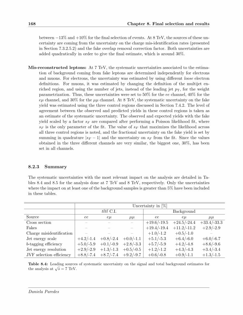
168 Chapter 8. Final selection and results
between −13% and +10% for the final selection of events. At 8 TeV, the sources of these un-certainty are coming from the uncertainty on the charge mis-identification rates (presentedin Section 7.3.2.5.2) and the fake overlap removal correction factor. Both uncertainties areadded quadratically in order to give the final estimate, which is around 30%.
Mis-reconstructed leptons: At 7 TeV, the systematic uncertainties associated to the estima-tion of background coming from fake leptons are determined independently for electronsand muons. For electrons, the uncertainty was estimated by using different loose electrondefinitions. For muons, it was estimated by changing the definition of the multijet en-riched region, and using the number of jets, instead of the leading jet pT, for the weightparametrization. Thus, these uncertainties were set to 50% for the ee channel, 40% for theeµ channel, and 30% for the µµ channel. At 8 TeV, the systematic uncertainty on the fakeyield was estimated using the three control regions discussed in Section 7.4.2. The level ofagreement between the observed and predicted yields in these control regions is taken asan estimate of the systematic uncertainty. The observed and expected yields with the fakeyield scaled by a factor sF are compared after performing a Poisson likelihood fit, wheresF is the only parameter of the fit. The value of sF that maximizes the likelihood acrossall three control regions is noted, and the fractional uncertainty on the fake yield is set bysumming in quadrature |sF − 1| and the uncertainty on sF from the fit. Since the valuesobtained in the three different channels are very similar, the biggest one, 30%, has beenset in all channels.
8.2.3 Summary
The systematic uncertainties with the most relevant impact on the analysis are detailed in Ta-bles 8.4 and 8.5 for the analysis done at 7 TeV and 8 TeV, respectively. Only the uncertaintieswhere the impact on at least one of the background samples is greater than 5% have been includedin these tables.
Uncertainty in [%]
tttt C.I. Background
Source ee eµ µµ ee eµ µµ
Cross section – – – +19.6/-19.5 +24.5/-24.4 +33.4/-33.3Fakes – – – +19.4/-19.4 +11.2/-11.2 +2.9/-2.9Charge misidentification – – – +1.0/-1.2 +0.5/-1.0 –Jet energy scale +4.2/-1.4 +0.8/-2.4 +0.0/-1.1 +5.1/-5.3 +6.4/-6.0 +6.0/-6.7b-tagging efficiency +5.0/-5.9 +0.1/-0.9 +2.8/-3.3 +5.7/-5.9 +4.2/-4.8 +8.6/-9.6Jet energy resolution +2.9/-2.9 +1.3/-1.3 +0.5/-0.5 +1.2/-1.2 +4.3/-4.3 +3.4/-3.4JVF selection efficiency +8.8/-7.4 +8.7/-7.4 +9.2/-9.7 +0.6/-0.8 +0.9/-1.1 +1.3/-1.5
Table 8.4: Leading sources of systematic uncertainty on the signal and total background estimates forthe analysis at
√s = 7 TeV.
Daniela Paredes

8.3. Results 169
Uncertainty in [%]
tttt C.I. Background
Source ee eµ µµ ee eµ µµ
Cross section – – – +16.6/-16.4 +22.4/-22.2 +30.2/-29.9Fakes – – – +7.2/-7.2 +1.1/-1.1 –Charge misidentification – – – +6.8/-6.8 +6.3/-6.3 –Jet energy scale +1.5/-2.8 +3.1/-3.3 +0.0/-2.4 +6.6/-9.6 +6.4/-6.2 +9.0/-8.0b-tagging efficiency +2.0/-2.9 +5.3/-8.2 +7.0/-8.2 +10.1/-9.2 +16.2/-15.2 +21.6/-19.8Jet energy resolution +1.1/-1.1 +1.2/-1.2 +1.6/-1.6 +1.7/-1.7 +1.5/-1.5 +0.9/-0.9JVF selection efficiency +8.8/-7.4 +2.4/-2.8 +2.2/-2.9 +1.0/-1.2 +1.6/-1.7 +2.0/-2.2
Table 8.5: Leading sources of systematic uncertainty on the signal and total background estimates forthe analysis at
√s = 8 TeV.
8.3 Results
In this section the results of the search of New Physics in events with four top quarks are pre-sented. First, a comparison between the expected background and data is done in Section 8.3.1.Then, the results of this comparison are interpreted in Section 8.3.2, where an upper limit onthe four tops production cross-section is set.
8.3.1 Data versus background expectation comparison
In the analysis performed with the data taken at√s = 7 TeV, and after applying the final
selection, 5.6± 1.7 events are expected from SM background, while 4 events have been observedin data. The details of the observed number of events are shown in Table 8.6, as well as the totalexpected number of background events for the three different channels. The total number ofexpected and observed events agree within uncertainties, which means that no significant excessis observed in data.
In the analysis performed with the data taken at√s = 8 TeV, 8 events are observed with
3.6 ± 1.3 expected from background. The details of the observed number of events are shownin Table 8.7, as well as the total expected number of background events for the three differentchannels. As can be seen, there is a small excess of observed events with respect to the totalbackground, which is coming from the eµ channel, since the yields in the ee and µµ channels areconsistent with the background expectations. For the eµ channel, the probability of observing sixor more events, given the expected background and the statistical and systematic uncertaintieson that expectation, is 3.9%. Since this probability is not small enough as to claim observation ofnew physics, the data is interpreted as constraining the four tops contact interaction productioncross-section.
The distributions of some kinematical variables after the final selection are shown in Ap-pendix C.
Daniela Paredes

170 Chapter 8. Final selection and results
ChannelBackgrounds ee eµ µµ
Q Mis-id 0.13± 0.04± 0.02 0.23± 0.04± 0.03 —Fakes 0.5± 1.1± 0.3 0.8± 1.1± 0.3 0.13± 0.13± 0.04
Diboson• WZ/ZZ(+jets) 0.19± 0.20± 0.07 0.34± 0.21± 0.13 0.28± 0.22± 0.10• W±W±jj 0.06± 0.03± 0.03 0.07± 0.03± 0.03 0.03± 0.02± 0.03
tt+W/Z• ttW (+jet) 0.23± 0.02± 0.07 0.79± 0.04± 0.24 0.57± 0.04± 0.18• ttZ(+jet) 0.17± 0.02± 0.09 0.61± 0.03± 0.31 0.33± 0.02± 0.17• ttW+W− 0.008± 0.001± 0.002 0.023± 0.001± 0.007 0.016± 0.001± 0.005
Total expected 1.3± 1.1± 0.3 2.9± 1.1± 0.5 1.36± 0.26± 0.27
Observed 2 2 0
Table 8.6: Expected number of background events with statistical (first) uncertainties and the dominantsystematic (second) uncertainties for the final signal selection at
√s = 7 TeV, compared to the number
of events observed in data.
ChannelSamples ee eµ µµ
Q Mis-id 0.16± 0.04± 0.05 0.41± 0.07± 0.12 —Fakes 0.18± 0.17± 0.05 0.07± 0.28± 0.02 < 1.14
Diboson• WZ/ZZ(+jets) < 0.11 0.01± 0.09± 0.01 < 0.11• W±W±jj < 0.03 0.18± 0.16± 0.07 < 0.03
tt+W/Z• ttW (+jet(s)) 0.31± 0.04± 0.12 0.93± 0.06± 0.35 0.65± 0.06± 0.25• ttZ(+jet(s)) 0.09± 0.02± 0.04 0.34± 0.04± 0.14 0.14± 0.02± 0.06• ttW+W− 0.012± 0.002± 0.005 0.039± 0.003± 0.016 0.024± 0.003± 0.01
Total 0.75± 0.21± 0.14 1.98± 0.35± 0.40 0.82± 1.15± 0.26
Observed 1 6 1
Table 8.7: Expected number of background events with statistical (first) uncertainties and the dominantsystematic (second) uncertainties for the final signal selection at
√s = 8 TeV, compared to the number
of events observed in data.
8.3.2 Interpretation of results: setting limit
Because no significant excess of events has been found in data, an upper limit at 95% C.L.on the four tops production cross-section has been computed using CLs method with the LLR(Log-Likelihood Ratio) as a test statistic. This is defined as
LLR = −2 logLs+b
Lb, (8.1)
Daniela Paredes

8.3. Results 171
where Ls+b (Lb) is the Poisson likelihood to observe the data under the signal-plus-background(background-only) hypothesis. Pseudo-experiments are generated under each of both hypothesis,taking into account statistical fluctuations of the total predictions according to Poisson statistics,as well as Gaussian fluctuations in the signal and background expectations describing the effectof systematic uncertainties. Correlations of the systematic uncertainties across the samples andchannels are taken into account. Each sample is statistically varied independently, using aGaussian function truncated at zero, in order to avoid negative contributions, in particular forthe samples which have a very low yield and a large statistical uncertainty. When no event isselected for a given sample, its yield is set to 0 with a statistical uncertainty given by the 68%C.L. upper limit using Poisson statistics, which is then rescaled to the data integrated luminosity.The fraction of s + b and b pseudo-experiments with LLR larger than the expected median orobserved LLR defines CLs+b and CLb for the expected and observed limits, respectively. Signalcross-sections for which CLs = CLs+b/CLb < 0.05 are considered excluded at the 95% C.L.
Single-bin counting experiments have been used to compute the limits. The combinedlimits have been calculated by considering each channel separately and summing their LLR.The corresponding upper limits on the four tops contact interaction production cross-section,channel by channel, and for the combination, obtained for the analyses performed at
√s = 7 TeV
and 8 TeV, and considering all the systematic uncertainties are shown in Tables 8.8 and 8.9,respectively.
95% C.L. upper limit [fb]
Channel Observed Expected 1σ range 2σ range
ee alone 473 474 280-706 280-954eµ alone 122 148 101-208 82-307µµ alone 113 150 112-241 112-244
Combination 61 90 63-133 39-194
Table 8.8: Upper limits at 95% C.L. obtained for each channel and their combination on σ(pp → tttt)for the contact interaction model at 7 TeV.
95% C.L. upper limit [fb]
Channel Observed Expected 1σ range 2σ range
ee alone 196 197 141-260 142-326eµ alone 133 66 53-97 42-133µµ alone 70 90 54-112 53-182
Combination 59 42 29-61 23-90
Table 8.9: Upper limits at 95% C.L. obtained for each channel and their combination on σ(pp → tttt)for the contact interaction model at 8 TeV.
In the analysis at√s = 8 TeV, and in the µµ channel, the estimate of the fakes contribution
is vanishing after the final selection. However, a statistical uncertainty on this yield is computedas the 68% C.L. upper limit. Since this background is extracted from data, this yield, andtherefore its uncertainty, are not rescaled to the luminosity. Thus, an upper limit of 1.14 events
Daniela Paredes
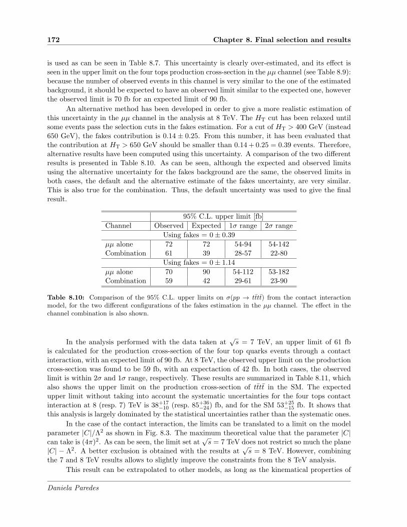
172 Chapter 8. Final selection and results
is used as can be seen in Table 8.7. This uncertainty is clearly over-estimated, and its effect isseen in the upper limit on the four tops production cross-section in the µµ channel (see Table 8.9):because the number of observed events in this channel is very similar to the one of the estimatedbackground, it should be expected to have an observed limit similar to the expected one, howeverthe observed limit is 70 fb for an expected limit of 90 fb.
An alternative method has been developed in order to give a more realistic estimation ofthis uncertainty in the µµ channel in the analysis at 8 TeV. The HT cut has been relaxed untilsome events pass the selection cuts in the fakes estimation. For a cut of HT > 400 GeV (instead650 GeV), the fakes contribution is 0.14 ± 0.25. From this number, it has been evaluated thatthe contribution at HT > 650 GeV should be smaller than 0.14 + 0.25 = 0.39 events. Therefore,alternative results have been computed using this uncertainty. A comparison of the two differentresults is presented in Table 8.10. As can be seen, although the expected and observed limitsusing the alternative uncertainty for the fakes background are the same, the observed limits inboth cases, the default and the alternative estimate of the fakes uncertainty, are very similar.This is also true for the combination. Thus, the default uncertainty was used to give the finalresult.
95% C.L. upper limit [fb]
Channel Observed Expected 1σ range 2σ range
Using fakes = 0± 0.39
µµ alone 72 72 54-94 54-142Combination 61 39 28-57 22-80
Using fakes = 0± 1.14
µµ alone 70 90 54-112 53-182Combination 59 42 29-61 23-90
Table 8.10: Comparison of the 95% C.L. upper limits on σ(pp → tttt) from the contact interactionmodel, for the two different configurations of the fakes estimation in the µµ channel. The effect in thechannel combination is also shown.
In the analysis performed with the data taken at√s = 7 TeV, an upper limit of 61 fb
is calculated for the production cross-section of the four top quarks events through a contactinteraction, with an expected limit of 90 fb. At 8 TeV, the observed upper limit on the productioncross-section was found to be 59 fb, with an expectaction of 42 fb. In both cases, the observedlimit is within 2σ and 1σ range, respectively. These results are summarized in Table 8.11, whichalso shows the upper limit on the production cross-section of tttt in the SM. The expectedupper limit without taking into account the systematic uncertainties for the four tops contactinteraction at 8 (resp. 7) TeV is 38+17
−10 (resp. 85+36−24) fb, and for the SM 53+25
−15 fb. It shows thatthis analysis is largely dominated by the statistical uncertainties rather than the systematic ones.
In the case of the contact interaction, the limits can be translated to a limit on the modelparameter |C|/Λ2 as shown in Fig. 8.3. The maximum theoretical value that the parameter |C|can take is (4π)2. As can be seen, the limit set at
√s = 7 TeV does not restrict so much the plane
|C| − Λ2. A better exclusion is obtained with the results at√s = 8 TeV. However, combining
the 7 and 8 TeV results allows to slightly improve the constraints from the 8 TeV analysis.
This result can be extrapolated to other models, as long as the kinematical properties of
Daniela Paredes
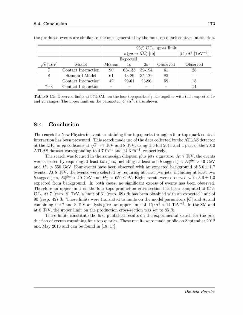
8.4. Conclusion 173
the produced events are similar to the ones generated by the four top quark contact interaction.
95% C.L. upper limit
σ(pp→ tttt) [fb] |C|/Λ2 [TeV−2]
Expected√s [TeV] Model Median 1σ 2σ Observed Observed
7 Contact Interaction 90 63-133 39-194 61 28
8 Standard Model 61 43-89 35-129 85 —Contact Interaction 42 29-61 23-90 59 15
7+8 Contact Interaction – – – – 14
Table 8.11: Observed limits at 95% C.L. on the four top quarks signals together with their expected 1σand 2σ ranges. The upper limit on the parameter |C|/Λ2 is also shown.
8.4 Conclusion
The search for New Physics in events containing four top quarks through a four-top quark contactinteraction has been presented. This search made use of the data collected by the ATLAS detectorat the LHC in pp collisions at
√s = 7 TeV and 8 TeV, using the full 2011 and a part of the 2012
ATLAS dataset corresponding to 4.7 fb−1 and 14.3 fb−1, respectively.The search was focused in the same-sign dilepton plus jets signature. At 7 TeV, the events
were selected by requiring at least two jets, including at least one b-tagged jet, EmissT > 40 GeV
and HT > 550 GeV. Four events have been observed with an expected background of 5.6 ± 1.7events. At 8 TeV, the events were selected by requiring at least two jets, including at least twob-tagged jets, Emiss
T > 40 GeV and HT > 650 GeV. Eight events were observed with 3.6 ± 1.3expected from background. In both cases, no significant excess of events has been observed.Therefore an upper limit on the four tops production cross-section has been computed at 95%C.L. At 7 (resp. 8) TeV, a limit of 61 (resp. 59) fb has been obtained with an expected limit of90 (resp. 42) fb. These limits were translated to limits on the model parameters |C| and Λ, andcombining the 7 and 8 TeV analysis gives an upper limit of |C|/Λ2 < 14 TeV−2. In the SM andat 8 TeV, the upper limit on the production cross-section was set to 85 fb.
These limits constitute the first published results on the experimental search for the pro-duction of events containing four top quarks. These results were made public on September 2012and May 2013 and can be found in [18, 17].
Daniela Paredes

174 Chapter 8. Final selection and results
[TeV]Λ
2 2.2 2.4 2.6 2.8 3 3.2 3.4
|C|
40
60
80
100
120
140
160
Excluded region at 95% CL
Observed limit at 95% CL
Expected limit at 95% CL
σ 1±Expected limit
σ 2±Expected limit
ATLAS Internal
-1Ldt = 4.7 fb∫ = 7 TeVs
(a)
[TeV]Λ
2 2.2 2.4 2.6 2.8 3 3.2 3.4
|C|
40
60
80
100
120
140
160
Excluded region at 95% CL
Observed limit at 95% CL
Expected limit at 95% CL
σ 1±Expected limit
σ 2±Expected limit
ATLAS Internal
-1Ldt = 14.3 fb∫
= 8 TeVs
(b)
[TeV]Λ
2 2.2 2.4 2.6 2.8 3 3.2 3.4
|C|
40
60
80
100
120
140
160
Excluded region at 95% CL
Observed limit at 95% CL
Expected limit at 95% CL
σ 1±Expected limit
σ 2±Expected limit
ATLAS Internal
= 7 TeVs, -1
Ldt = 4.7 fb∫ = 8 TeVs,
-1Ldt = 14.3 fb∫
(c)
Figure 8.3: Observed and expected limits obtained in the analysis performed with the data taken at√s = 7 TeV (a), 8 TeV (b), and combination of both (c), on the contact interaction model parameters |C|
and Λ. The region above the observed line is excluded at 95% C.L. The signal sample has been generatedwith a value of C/Λ2 = −4π TeV−2. Below Λ = 2 TeV the low energy effective field theory with the fourtops contact interaction is not expected to be valid anymore.
Daniela Paredes

Conclusion
Currently, the LHC is capable of colliding particles up to energies never reached by the humanbeing, providing access to a yet unexplored energy regime. It is hoped that it clarifies at leastsome of the questions not answered by the Standard Model and helps to construct that sowished Theory of Everything. Many beyond-the-SM theories could be tested at the LHC. Someof these theories predict final states involving four top quarks (tttt). Therefore, this kind ofevents provides an open window in order to look for new physics phenomena.
In this thesis, two topics have been treated. The main one has been focused in the searchfor New Physics in events with four top quarks in a model-independent approach, using the datacollected by the ATLAS detector at LHC in pp collisions at
√s = 7 TeV and 8 TeV during 2011
and a part of 2012, corresponding to 4.7 fb−1 and 14.3 fb−1, respectively. The other topic isrelated to the LASER calibration system of the ATLAS Tile calorimeter.
For this last topic, the stability and linearity of the electronics of the photodiodes, usedto measure the intensity of the laser light, was monitored using the data collected between 2011and the first months of 2013. The monitoring activity was split in four different periods, wheretwo periods are separated by a hardware intervention. One of these interventions in particularmade the system much more stable: the change of the motherboard inside the photodiodes box.After this intervention (made on July 6th, 2011) the photodiodes absolute response was stablewithin a range of 0.5%. This measurement was done with a new method used to determinethe stability of the alpha spectra: the scale factor. It was demonstrated that this method ismore stable than the normalized mean value (default method used in studies previous to thisone). To finalize this part, the study of the photodiodes response is the first step towards theunderstanding of the LASER system. This calibration system is crucial to monitor correctly theTile calorimeter readout electronics, which is essential for measuring the energy and direction ofthe hadrons produced in the collisions, as well as the missing transverse momentum.
Concerning the search for New Physics in events with four top quarks, the analysis wasfocused in a final state with two leptons (electrons or muons) with the same electric charge. Thischannel was chosen since this kind of events is rarely produced in Standard Model processes.Different event selections were used in each one of the two analyses performed at 7 TeV and8 TeV. In both cases, no significant excess of events has been observed. Therefore an upper limiton the four tops contact interaction production cross-section has been computed at 95% C.L.At 7 (resp. 8) TeV, a limit of 61 (resp. 59) fb has been obtained with an expected limit of 90(resp. 42) fb. In the SM and at 8 TeV, the upper limit on the production cross-section was set to
Daniela Paredes

176 CONCLUSION
85 fb with an expected limit of 61 fb. In the case of the contact interaction, the upper limit on theproduction cross-section can be translated to a limit on the model parameter |C|/Λ2. Combiningthe 7 and 8 TeV analyses the upper limit on this parameter is |C|/Λ2 < 14 TeV−2. The limitspresented in this thesis constitute the first published results on the experimental search for theproduction of events containing four top quarks. They can be found in [18, 17].
Although no new physics phenomena were observed in this analysis, the model-independentnature of the framework used to set the upper limits on the four tops contact interaction produc-tion cross-sections allows to extrapolate to other models, as long as the kinematical properties ofthe produced events are similar to the ones generated by the four top quark contact interaction.
About the estimation of the background coming from the mis-identification of the electroncharge, a new method was developed in order to take into account the dependence on the elec-tron pT of the mis-identification rates. Basically, the likelihood method is kept as the baseline inorder to compute the rates as a function of |η|, which are then corrected using a pT dependentfactor extracted from tt simulated events. The regions used by the side-band method to extractthe background from the Z-peak have been also redefined. It now takes into account the shiftof the same-sign invariant mass distribution to lower values with respect to the opposite-signdistribution. The computation of the systematic uncertainty has also been improved. Differentsources of systematics are now considered, which are related to the change of the Z peak defini-tion, the use of different tt samples to extract the pT correction factor, the differences betweenthe measured and true rates extracted from simulated samples, and the statistical uncertaintiescoming from the likelihood method and the pT correction.
Future improvements of the present analysis can include an event selection optimizationperformed channel by channel (i.e. ee, eµ and µµ). As it was shown, the analysis is largelydominated by the statistical uncertainties. Thus, the inclusion of more data, providing muchmore statistics could help to reduce the impact of these uncertainties, and therefore to set strongerlimits on the production cross-sections. The analysis will be redone with the full 2012 dataset,corresponding to 20.3 fb−1, which does not increase so much the statistics, but which will allow,in principle, to provide better measurements. The analysis could also be extended to otherchannels (i.e. not only same-sign dilepton), with a final result coming from the combination ofall these channels.
Finally, after the long shutdown, it is expected that the LHC delivers around∼ 75−100 fb−1
over a period of three years at a center-of-mass energy of 13−14 TeV. In these conditions, the SMproduction of four top quarks (σtttt ∼ 7− 11 fb) will not be negligible anymore, and hundreds offour tops events are expected to be produced at the LHC. It will therefore be possible to measurethe four tops events production cross-section and compare it to the SM prediction in order toconstrain a possible enhancement from New Physics.
Daniela Paredes

Appendices
Daniela Paredes


Appendix A
Study of the four top eventskinematic
This appendix is dedicated to the study of the four top events kinematic at the parton level.These studies were done by E. Busato.
A.1 Four top events kinematic for large Mρ
In order to demonstrate that the event kinematics do not depend on Mρ and gρ when Mρ islarge (i.e. when the four top interaction can be approximated by a contact interaction), threedifferent configurations were compared:
• gρ = 10√8π, Mρ = 10 TeV,
• gρ = 100√8π, Mρ = 100 TeV (values used to generate the signal in this analysis),
• gρ = 1000√8π, Mρ = 1000 TeV.
The Fig. A.1 shows the inclusive distributions of η and energy at parton level for topquarks, W bosons, electrons and muons, neutrinos and b quarks for the configurations studied.It demonstrates that the event kinematics is the same for the three configurations, and thatit does not depend on the values of Mρ and gρ when Mρ is large. That means that the signalacceptance is the same for allMρ in the contact interaction regime, and that only the cross-sectiondepends on the parameters Mρ and gρ.
A.2 Four top events kinematic for low Mρ and comparison tothe large Mρ case
This section is dedicated to give an estimation of the signal acceptance for lowMρ and comparingthe result to the acceptance for large Mρ. In order to do that, the following configurations werecompared:
Daniela Paredes

180 Chapter A. Study of the four top events kinematic
• gρ =√2π, Mρ = 500 GeV,
• gρ =√8π, Mρ = 1 TeV,
• gρ = 10√8π, Mρ = 10 TeV,
• gρ = 100√8π, Mρ = 100 TeV (values used to generate the signal in this analysis),
• Standard Model.
A comparison of the first three configurations is shown in Fig. A.2. As can be seen, asMρ decreases, the objets get softer, meaning that the event kinematic starts to change. Thesechanges are quantified at parton level by computing the acceptances. These values are shownin Table A.1 for the µµ channel. Similar results are obtained in ee and eµ channel. Due tothe absence of trigger, reconstruction and identification efficiencies, all analysis cuts cannot beapplied. Only these relevant at the parton level were therefore applied. For that reason, theacceptances calculated at the parton level are very different from the ones used in the analysis,which are computed after full detector simulation. Thus, the information of interest residesin their relative differences rather than in their absolute values. This way, the acceptance forMρ = 500 GeV is about 30% lower than the one in the contact interaction regime. It meansthat upper limits on the production cross-section for low Mρ are approximately 30% worse thanin the large Mρ case. However, it should be noted that cross sections generally increase as Mρ
decreases, so the analysis sensitivity decreases by less than 30%. Table A.1 also shows that theacceptance for the Standard Model production of 4 top events is close to the one for gρ = 100
√8π,
Mρ = 100 TeV. Summarizing, even if the analysis described is based on a large value of Mρ, itis also sensitive to configurations where the contact interaction approximation is not valid.
gρ =√2π gρ =
√8π gρ = 10
√8π gρ = 100
√8π
Cut Mρ = 500 GeV Mρ = 1 TeV Mρ = 10 TeV Mρ = 100 TeV SM
≥ 2 muons 4.6 4.7 4.9 5.1 4.8Same sign 1.6 1.8 1.9 2 1.9Z veto 1.4 1.6 1.7 1.9 1.6Njets ≥ 2 1.4 1.6 1.7 1.9 1.6
EmissT > 40 GeV 1.1 1.4 1.5 1.7 1.5HT > 500 GeV 1 1.3 1.4 1.5 1.3
Table A.1: Parton level acceptance (in %) for all the configurations described in the text after analysiscuts in the µµ channel.
Daniela Paredes

A.2. Four top events kinematic for low Mρ and comparison to the large Mρ case181
η
-4 -3 -2 -1 0 1 2 3 40
0.01
0.02
0.03
0.04
0.05
0.06
0.07
0.08particle : top
= 10 TeV ρ
; Mπ8= 100 ρ
g
= 100 TeV ρ
; Mπ8= 100 ρ
g
= 1000 TeV ρ
; Mπ8= 100 ρ
g
E [GeV]
0 200 400 600 800 1000 1200 14000
0.02
0.04
0.06
0.08
0.1
0.12
1.3±mean = 422.6
1.3±mean = 421.2
1.3±mean = 421.2
particle : top
= 10 TeV ρ
; Mπ8= 100 ρ
g
= 100 TeV ρ
; Mπ8= 100 ρ
g
= 1000 TeV ρ
; Mπ8= 100 ρ
g
(a)
η
-4 -3 -2 -1 0 1 2 3 40
0.01
0.02
0.03
0.04
0.05
0.06
0.07
0.08 particle : W
= 10 TeV ρ
; Mπ8= 100 ρ
g
= 100 TeV ρ
; Mπ8= 100 ρ
g
= 1000 TeV ρ
; Mπ8= 100 ρ
g
E [GeV]
0 200 400 600 800 1000 1200 14000
0.02
0.04
0.06
0.08
0.1
0.12
0.14
0.16
0.18
1.0±mean = 257.7
1.0±mean = 258.0
1.0±mean = 258.2
particle : W
= 10 TeV ρ
; Mπ8= 100 ρ
g
= 100 TeV ρ
; Mπ8= 100 ρ
g
= 1000 TeV ρ
; Mπ8= 100 ρ
g
(b)
η
-4 -3 -2 -1 0 1 2 3 40
0.02
0.04
0.06
0.08
0.1µparticle : e,
= 10 TeV ρ
; Mπ8= 100 ρ
g
= 100 TeV ρ
; Mπ8= 100 ρ
g
= 1000 TeV ρ
; Mπ8= 100 ρ
g
E [GeV]
0 200 400 600 800 1000 1200 14000
0.05
0.1
0.15
0.2
0.25
0.3
1.4±mean = 116.0
1.4±mean = 115.0
1.5±mean = 118.3
µparticle : e,
= 10 TeV ρ
; Mπ8= 100 ρ
g
= 100 TeV ρ
; Mπ8= 100 ρ
g
= 1000 TeV ρ
; Mπ8= 100 ρ
g
(c)
Daniela Paredes
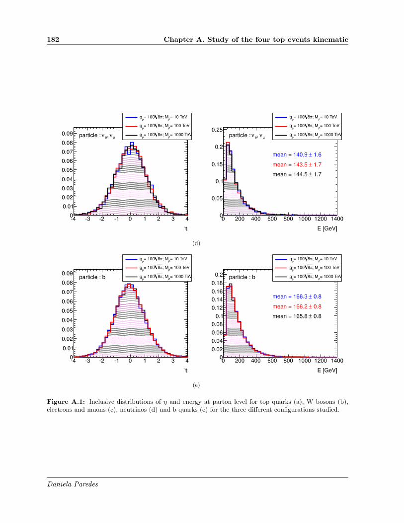
182 Chapter A. Study of the four top events kinematic
η
-4 -3 -2 -1 0 1 2 3 40
0.01
0.02
0.03
0.04
0.05
0.06
0.07
0.08
0.09µν, eνparticle :
= 10 TeV ρ
; Mπ8= 100 ρ
g
= 100 TeV ρ
; Mπ8= 100 ρ
g
= 1000 TeV ρ
; Mπ8= 100 ρ
g
E [GeV]
0 200 400 600 800 1000 1200 14000
0.05
0.1
0.15
0.2
0.25
1.6±mean = 140.9
1.7±mean = 143.5
1.7±mean = 144.5
µν, eνparticle :
= 10 TeV ρ
; Mπ8= 100 ρ
g
= 100 TeV ρ
; Mπ8= 100 ρ
g
= 1000 TeV ρ
; Mπ8= 100 ρ
g
(d)
η
-4 -3 -2 -1 0 1 2 3 40
0.01
0.02
0.03
0.04
0.05
0.06
0.07
0.08
0.09particle : b
= 10 TeV ρ
; Mπ8= 100 ρ
g
= 100 TeV ρ
; Mπ8= 100 ρ
g
= 1000 TeV ρ
; Mπ8= 100 ρ
g
E [GeV]
0 200 400 600 800 1000 1200 14000
0.02
0.04
0.06
0.08
0.1
0.12
0.14
0.16
0.18
0.2
0.8±mean = 166.3
0.8±mean = 166.2
0.8±mean = 165.8
particle : b
= 10 TeV ρ
; Mπ8= 100 ρ
g
= 100 TeV ρ
; Mπ8= 100 ρ
g
= 1000 TeV ρ
; Mπ8= 100 ρ
g
(e)
Figure A.1: Inclusive distributions of η and energy at parton level for top quarks (a), W bosons (b),electrons and muons (c), neutrinos (d) and b quarks (e) for the three different configurations studied.
Daniela Paredes

A.2. Four top events kinematic for low Mρ and comparison to the large Mρ case183
η
-4 -3 -2 -1 0 1 2 3 40
0.01
0.02
0.03
0.04
0.05
0.06
0.07particle : top
= 500 GeV ρ
; Mπ2= ρ
g
= 1 TeV ρ
; Mπ8= ρ
g
= 10 TeV ρ
; Mπ8= 10 ρ
g
E [GeV]
0 200 400 600 800 1000 1200 14000
0.02
0.04
0.06
0.08
0.1
0.12
0.14
0.16
1.1±mean = 362.0
1.3±mean = 408.6
1.3±mean = 422.4
particle : top
= 500 GeV ρ
; Mπ2= ρ
g
= 1 TeV ρ
; Mπ8= ρ
g
= 10 TeV ρ
; Mπ8= 10 ρ
g
(a)
η
-4 -3 -2 -1 0 1 2 3 40
0.01
0.02
0.03
0.04
0.05
0.06
0.07
0.08particle : W
= 500 GeV ρ
; Mπ2= ρ
g
= 1 TeV ρ
; Mπ8= ρ
g
= 10 TeV ρ
; Mπ8= 10 ρ
g
E [GeV]
0 200 400 600 800 1000 1200 14000
0.02
0.04
0.06
0.08
0.1
0.12
0.14
0.16
0.18
0.2
0.22
0.9±mean = 221.6
1.0±mean = 250.4
1.0±mean = 258.4
particle : W
= 500 GeV ρ
; Mπ2= ρ
g
= 1 TeV ρ
; Mπ8= ρ
g
= 10 TeV ρ
; Mπ8= 10 ρ
g
(b)
η
-4 -3 -2 -1 0 1 2 3 40
0.01
0.02
0.03
0.04
0.05
0.06
0.07
0.08
0.09µparticle : e,
= 500 GeV ρ
; Mπ2= ρ
g
= 1 TeV ρ
; Mπ8= ρ
g
= 10 TeV ρ
; Mπ8= 10 ρ
g
E [GeV]
0 200 400 600 800 1000 1200 14000
0.05
0.1
0.15
0.2
0.25
0.3
1.2±mean = 97.6
1.4±mean = 113.6
1.4±mean = 114.4
µparticle : e,
= 500 GeV ρ
; Mπ2= ρ
g
= 1 TeV ρ
; Mπ8= ρ
g
= 10 TeV ρ
; Mπ8= 10 ρ
g
(c)
Daniela Paredes

184 Chapter A. Study of the four top events kinematic
η
-4 -3 -2 -1 0 1 2 3 40
0.01
0.02
0.03
0.04
0.05
0.06
0.07
0.08
0.09µν, eνparticle :
= 500 GeV ρ
; Mπ2= ρ
g
= 1 TeV ρ
; Mπ8= ρ
g
= 10 TeV ρ
; Mπ8= 10 ρ
g
E [GeV]
0 200 400 600 800 1000 1200 14000
0.05
0.1
0.15
0.2
0.25
1.4±mean = 124.0
1.6±mean = 140.9
1.6±mean = 141.7
µν, eνparticle :
= 500 GeV ρ
; Mπ2= ρ
g
= 1 TeV ρ
; Mπ8= ρ
g
= 10 TeV ρ
; Mπ8= 10 ρ
g
(d)
η
-4 -3 -2 -1 0 1 2 3 40
0.01
0.02
0.03
0.04
0.05
0.06
0.07
0.08
0.09particle : b
= 500 GeV ρ
; Mπ2= ρ
g
= 1 TeV ρ
; Mπ8= ρ
g
= 10 TeV ρ
; Mπ8= 10 ρ
g
E [GeV]
0 200 400 600 800 1000 1200 14000
0.02
0.04
0.06
0.08
0.1
0.12
0.14
0.16
0.18
0.2
0.22
0.24
0.7±mean = 141.9
0.8±mean = 160.5
0.8±mean = 165.9
particle : b
= 500 GeV ρ
; Mπ2= ρ
g
= 1 TeV ρ
; Mπ8= ρ
g
= 10 TeV ρ
; Mπ8= 10 ρ
g
(e)
Figure A.2: Inclusive distributions of η and energy at parton level for top quarks (a), W bosons (b),electrons and muons (c), neutrinos (d) and b quarks (e) for (gρ =
√2π,Mρ = 500 GeV), (gρ =
√8π,Mρ =
1 TeV) and (gρ = 10√8π,Mρ = 10 TeV).
Daniela Paredes

Appendix B
Systematic uncertainties used in thelimit computation
B.1 Uncertainties affecting the Monte Carlo samples
The list of the systematic uncertainties affecting the Monte Carlo samples used for the limit com-putation on the four tops production cross-section at 7 (resp. 8) TeV can be found in Tables B.1,B.2 and B.3 (resp. B.4, B.5 and B.6) for the ee, eµ and µµ channels, respectively. In the tables,the name of the uncertainties follows the following notation:
• BTagSF(b,c,l): Uncertainties on the b-tagging, c-tagging and light-jets tagging scalefactors.
• EE(R,S): Uncertainties on the electron energy resolution and electron energy scale.
• JEFFSF: Uncertainty on the jet efficiency scale factor.
• JERSF: Uncertainty on the jet energy resolution scale factor.
• JES: Uncertainty on jet energy scale.
• JVFSF: Uncertainty on the JVF scale factor.
• Luminosity: Uncertainty on the integrated luminosity.
• MuER(ID,MS): Uncertainty on the muon energy resolution coming from the inner de-tector (ID) and muon spectrometer (MS).
• MuES: Uncertainty on the muon energy scale.
• PDF: Uncertainty on the PDF.
• SSW(id,rec,trg): Uncertainty on the lepton scale factors of the same-sign pair comingfrom identification (id), reconstruction (rec) and trigger (trg).
• XS: Uncertainty on the cross-section production.
Daniela Paredes
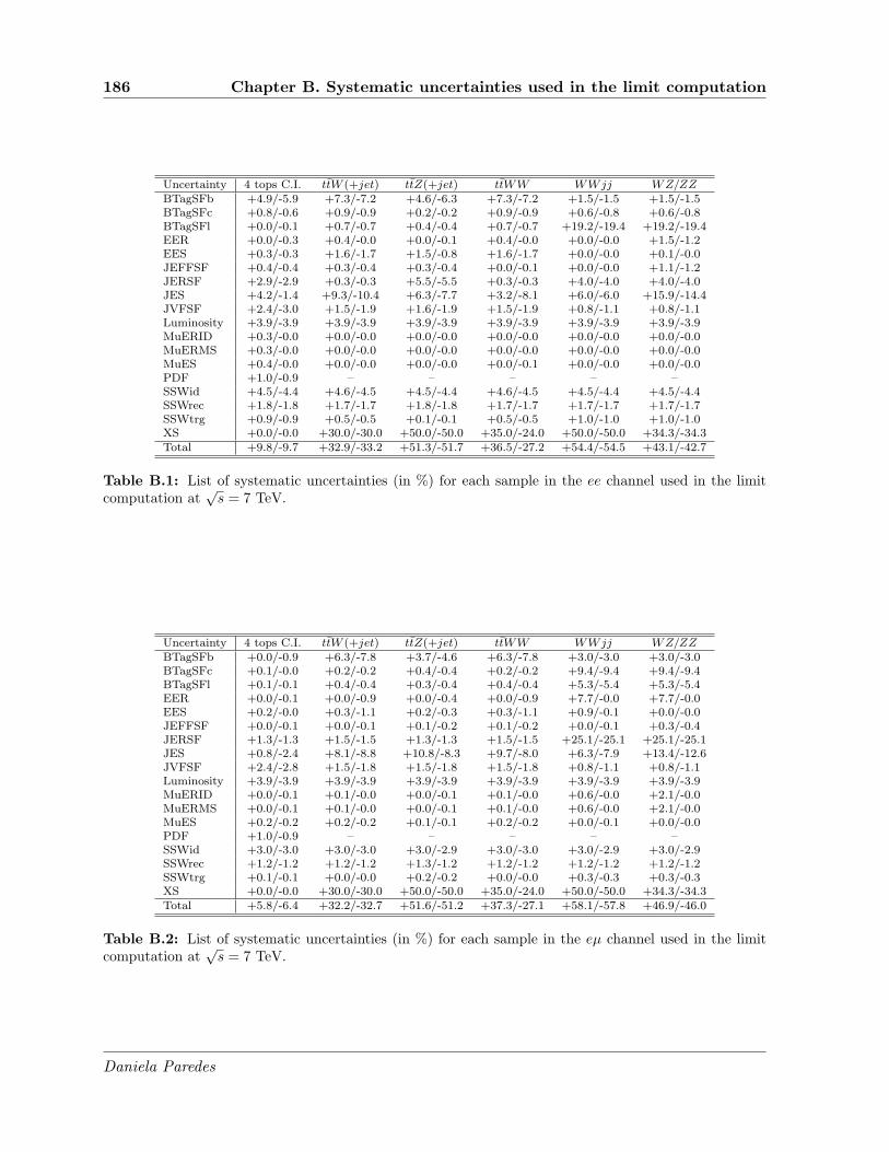
186 Chapter B. Systematic uncertainties used in the limit computation
Uncertainty 4 tops C.I. ttW (+jet) ttZ(+jet) ttWW WWjj WZ/ZZBTagSFb +4.9/-5.9 +7.3/-7.2 +4.6/-6.3 +7.3/-7.2 +1.5/-1.5 +1.5/-1.5BTagSFc +0.8/-0.6 +0.9/-0.9 +0.2/-0.2 +0.9/-0.9 +0.6/-0.8 +0.6/-0.8BTagSFl +0.0/-0.1 +0.7/-0.7 +0.4/-0.4 +0.7/-0.7 +19.2/-19.4 +19.2/-19.4EER +0.0/-0.3 +0.4/-0.0 +0.0/-0.1 +0.4/-0.0 +0.0/-0.0 +1.5/-1.2EES +0.3/-0.3 +1.6/-1.7 +1.5/-0.8 +1.6/-1.7 +0.0/-0.0 +0.1/-0.0JEFFSF +0.4/-0.4 +0.3/-0.4 +0.3/-0.4 +0.0/-0.1 +0.0/-0.0 +1.1/-1.2JERSF +2.9/-2.9 +0.3/-0.3 +5.5/-5.5 +0.3/-0.3 +4.0/-4.0 +4.0/-4.0JES +4.2/-1.4 +9.3/-10.4 +6.3/-7.7 +3.2/-8.1 +6.0/-6.0 +15.9/-14.4JVFSF +2.4/-3.0 +1.5/-1.9 +1.6/-1.9 +1.5/-1.9 +0.8/-1.1 +0.8/-1.1Luminosity +3.9/-3.9 +3.9/-3.9 +3.9/-3.9 +3.9/-3.9 +3.9/-3.9 +3.9/-3.9MuERID +0.3/-0.0 +0.0/-0.0 +0.0/-0.0 +0.0/-0.0 +0.0/-0.0 +0.0/-0.0MuERMS +0.3/-0.0 +0.0/-0.0 +0.0/-0.0 +0.0/-0.0 +0.0/-0.0 +0.0/-0.0MuES +0.4/-0.0 +0.0/-0.0 +0.0/-0.0 +0.0/-0.1 +0.0/-0.0 +0.0/-0.0PDF +1.0/-0.9 – – – – –SSWid +4.5/-4.4 +4.6/-4.5 +4.5/-4.4 +4.6/-4.5 +4.5/-4.4 +4.5/-4.4SSWrec +1.8/-1.8 +1.7/-1.7 +1.8/-1.8 +1.7/-1.7 +1.7/-1.7 +1.7/-1.7SSWtrg +0.9/-0.9 +0.5/-0.5 +0.1/-0.1 +0.5/-0.5 +1.0/-1.0 +1.0/-1.0XS +0.0/-0.0 +30.0/-30.0 +50.0/-50.0 +35.0/-24.0 +50.0/-50.0 +34.3/-34.3Total +9.8/-9.7 +32.9/-33.2 +51.3/-51.7 +36.5/-27.2 +54.4/-54.5 +43.1/-42.7
Table B.1: List of systematic uncertainties (in %) for each sample in the ee channel used in the limitcomputation at
√s = 7 TeV.
Uncertainty 4 tops C.I. ttW (+jet) ttZ(+jet) ttWW WWjj WZ/ZZBTagSFb +0.0/-0.9 +6.3/-7.8 +3.7/-4.6 +6.3/-7.8 +3.0/-3.0 +3.0/-3.0BTagSFc +0.1/-0.0 +0.2/-0.2 +0.4/-0.4 +0.2/-0.2 +9.4/-9.4 +9.4/-9.4BTagSFl +0.1/-0.1 +0.4/-0.4 +0.3/-0.4 +0.4/-0.4 +5.3/-5.4 +5.3/-5.4EER +0.0/-0.1 +0.0/-0.9 +0.0/-0.4 +0.0/-0.9 +7.7/-0.0 +7.7/-0.0EES +0.2/-0.0 +0.3/-1.1 +0.2/-0.3 +0.3/-1.1 +0.9/-0.1 +0.0/-0.0JEFFSF +0.0/-0.1 +0.0/-0.1 +0.1/-0.2 +0.1/-0.2 +0.0/-0.1 +0.3/-0.4JERSF +1.3/-1.3 +1.5/-1.5 +1.3/-1.3 +1.5/-1.5 +25.1/-25.1 +25.1/-25.1JES +0.8/-2.4 +8.1/-8.8 +10.8/-8.3 +9.7/-8.0 +6.3/-7.9 +13.4/-12.6JVFSF +2.4/-2.8 +1.5/-1.8 +1.5/-1.8 +1.5/-1.8 +0.8/-1.1 +0.8/-1.1Luminosity +3.9/-3.9 +3.9/-3.9 +3.9/-3.9 +3.9/-3.9 +3.9/-3.9 +3.9/-3.9MuERID +0.0/-0.1 +0.1/-0.0 +0.0/-0.1 +0.1/-0.0 +0.6/-0.0 +2.1/-0.0MuERMS +0.0/-0.1 +0.1/-0.0 +0.0/-0.1 +0.1/-0.0 +0.6/-0.0 +2.1/-0.0MuES +0.2/-0.2 +0.2/-0.2 +0.1/-0.1 +0.2/-0.2 +0.0/-0.1 +0.0/-0.0PDF +1.0/-0.9 – – – – –SSWid +3.0/-3.0 +3.0/-3.0 +3.0/-2.9 +3.0/-3.0 +3.0/-2.9 +3.0/-2.9SSWrec +1.2/-1.2 +1.2/-1.2 +1.3/-1.2 +1.2/-1.2 +1.2/-1.2 +1.2/-1.2SSWtrg +0.1/-0.1 +0.0/-0.0 +0.2/-0.2 +0.0/-0.0 +0.3/-0.3 +0.3/-0.3XS +0.0/-0.0 +30.0/-30.0 +50.0/-50.0 +35.0/-24.0 +50.0/-50.0 +34.3/-34.3Total +5.8/-6.4 +32.2/-32.7 +51.6/-51.2 +37.3/-27.1 +58.1/-57.8 +46.9/-46.0
Table B.2: List of systematic uncertainties (in %) for each sample in the eµ channel used in the limitcomputation at
√s = 7 TeV.
Daniela Paredes

B.1. Uncertainties affecting the Monte Carlo samples 187
Uncertainty 4 tops C.I. ttW (+jet) ttZ(+jet) ttWW WWjj WZ/ZZBTagSFb +2.8/-3.3 +3.8/-5.5 +5.4/-6.1 +3.8/-5.5 +0.8/-0.8 +0.8/-0.8BTagSFc +0.4/-0.4 +0.2/-0.2 +0.6/-0.7 +0.2/-0.2 +0.1/-0.2 +0.1/-0.2BTagSFl +0.0/-0.0 +0.2/-0.2 +0.3/-0.3 +0.2/-0.2 +24.6/-24.9 +24.6/-24.9EER +0.0/-0.0 +0.0/-0.0 +0.0/-0.0 +0.0/-0.0 +0.0/-0.0 +0.0/-0.0EES +0.0/-0.0 +0.0/-0.1 +0.0/-0.0 +0.0/-0.0 +0.0/-0.0 +0.0/-0.0JEFFSF +0.2/-0.3 +0.0/-0.1 +0.6/-0.7 +0.1/-0.2 +0.0/-0.0 +0.4/-0.5JERSF +0.5/-0.5 +1.0/-1.0 +6.4/-6.4 +1.0/-1.0 +6.3/-6.3 +6.3/-6.3JES +0.0/-1.1 +8.1/-9.9 +5.4/-6.9 +5.1/-4.0 +0.5/-10.9 +6.0/-2.7JVFSF +2.2/-2.9 +1.5/-1.8 +1.4/-1.8 +1.5/-1.8 +1.2/-1.3 +1.2/-1.3Luminosity +3.9/-3.9 +3.9/-3.9 +3.9/-3.9 +3.9/-3.9 +3.9/-3.9 +3.9/-3.9MuERID +0.0/-0.0 +0.0/-0.0 +0.0/-0.9 +0.0/-0.0 +1.1/-1.1 +3.3/-0.6MuERMS +0.0/-0.0 +0.0/-0.0 +0.0/-0.9 +0.0/-0.0 +1.1/-1.1 +3.3/-0.6MuES +0.4/-0.4 +0.3/-0.3 +0.6/-0.6 +0.3/-0.3 +0.0/-0.0 +0.0/-0.0PDF +1.0/-0.9 – – – – –SSWid +1.5/-1.5 +1.5/-1.5 +1.5/-1.5 +1.5/-1.5 +1.5/-1.5 +1.5/-1.5SSWrec +0.7/-0.7 +0.7/-0.7 +0.7/-0.7 +0.7/-0.7 +0.7/-0.7 +0.7/-0.7SSWtrg +0.5/-0.5 +0.3/-0.4 +0.5/-0.5 +0.3/-0.4 +2.3/-2.2 +2.3/-2.2XS +0.0/-0.0 +30.0/-30.0 +50.0/-50.0 +35.0/-24.0 +50.0/-50.0 +34.3/-34.3Total +5.6/-6.2 +31.6/-32.4 +51.2/-51.5 +35.9/-25.4 +56.3/-57.5 +43.6/-43.2
Table B.3: List of systematic uncertainties (in %) for each sample in the µµ channel used in the limitcomputation at
√s = 7 TeV.
4 tops SM 4 tops C.I. ttW (jet(s)) ttZ(jet(s)) WWjj ttWW WZ/ZZBTagSFb +6.2/-7.1 +0.0/-2.2 +19.1/-17.4 +15.6/-14.3 +0.0/+0.0 +16.9/-16.1 +0.0/+0.0BTagSFc +3.0/-2.7 +2.0/-1.9 +2.1/-2.2 +1.1/-0.5 +0.0/+0.0 +0.6/-0.8 +0.0/+0.0BTagSFl +0.8/-0.8 +0.1/-0.1 +0.9/-0.8 +0.3/-0.3 +0.0/+0.0 +0.3/-0.3 +0.0/+0.0EER +0.0/-0.4 +1.2/-0.0 +0.0/-1.0 +0.0/-0.0 +0.0/+0.0 +1.2/-0.0 +0.0/+0.0EES +0.0/-0.0 +0.0/-0.0 +0.0/-0.0 +0.0/-0.0 +0.0/+0.0 +0.0/-0.0 +0.0/+0.0JEFFSF +0.0/-0.0 +0.0/-0.0 +0.0/-0.0 +0.0/-0.0 +0.0/+0.0 +0.0/-0.0 +0.0/+0.0JERSF +2.2/-2.2 +1.1/-1.1 +2.6/-2.6 +5.2/-5.2 +0.0/+0.0 +2.7/-2.7 +0.0/+0.0JES +5.2/-7.8 +1.5/-2.8 +12.9/-12.0 +9.0/-26.1 +0.0/+0.0 +10.0/-9.4 +12.2/+0.0JVFSF +8.3/-7.0 +8.8/-7.4 +1.8/-2.2 +2.2/-2.3 +0.0/+0.0 +2.2/-2.3 +0.0/+0.0Luminosity +3.6/-3.6 +3.6/-3.6 +3.6/-3.6 +3.6/-3.6 +3.6/-3.6 +3.6/-3.6 +3.6/-3.6MuERID +0.0/-0.0 +0.0/-0.0 +0.0/-0.0 +0.0/-0.0 +0.0/+0.0 +0.0/-0.0 +0.0/+0.0MuERMS +0.0/-0.0 +0.0/-0.0 +0.0/-0.0 +0.0/-0.0 +0.0/+0.0 +0.0/-0.0 +0.0/+0.0MuES +0.0/-0.0 +0.0/-0.0 +0.0/-0.0 +0.0/-0.0 +0.0/+0.0 +0.0/-0.0 +0.0/+0.0PDF +1.0/-0.9 +1.0/-0.9 – – – – –SSWid +4.8/-4.7 +4.8/-4.7 +4.8/-4.7 +4.8/-4.7 +0.0/+0.0 +4.8/-4.7 +0.0/+0.0SSWrec +1.3/-1.3 +1.4/-1.3 +1.3/-1.3 +1.4/-1.4 +0.0/+0.0 +1.3/-1.3 +0.0/+0.0SSWtrg +0.0/-0.0 +0.5/-0.5 +0.5/-0.5 +0.2/-0.2 +0.0/+0.0 +0.2/-0.2 +0.0/+0.0XS – – +30.0/-30.0 +30.0/-30.0 +25.0/-25.0 +38.0/-26.0 +34.3/-34.3Total +13.6/-14.6 +11.2/-10.5 +38.5/-37.4 +36.0/-43.1 +25.3/-25.3 +43.4/-32.7 +36.6/-34.5
Table B.4: List of systematic uncertainties (in %) for each sample in the ee channel used in the limitcomputation at
√s = 8 TeV.
Daniela Paredes

188 Chapter B. Systematic uncertainties used in the limit computation
4 tops SM 4 tops C.I. ttW (jet(s)) ttZ(jet(s)) WWjj ttWW WZ/ZZBTagSFb +8.4/-9.9 +2.7/-6.2 +20.9/-19.2 +18.3/-17.0 +0.0/-0.0 +15.8/-14.9 +13.5/-13.5BTagSFc +1.3/-1.3 +4.6/-5.3 +4.3/-4.9 +4.3/-3.2 +15.6/-15.6 +0.0/-0.9 +11.3/-13.4BTagSFl +0.3/-0.3 +0.0/-0.1 +1.2/-1.2 +1.5/-1.4 +22.6/-22.8 +0.8/-0.8 +0.6/-0.6EER +0.0/-0.1 +0.0/-0.0 +1.5/-0.0 +0.5/-1.2 +0.1/-0.1 +0.0/-0.5 +0.0/-0.0EES +0.0/-0.0 +0.0/-0.0 +0.0/-0.0 +0.0/-0.0 +0.0/-0.0 +0.0/-0.0 +0.0/-0.0JEFFSF +0.0/-0.0 +0.0/-0.0 +0.2/-0.2 +0.0/-0.0 +0.0/-0.0 +0.0/-0.0 +0.0/-0.0JERSF +0.2/-0.2 +1.2/-1.2 +0.2/-0.2 +4.9/-4.9 +0.1/-0.1 +4.1/-4.1 +100.0/-100.0JES +4.2/-7.1 +3.1/-3.3 +7.1/-8.0 +17.0/-12.8 +0.0/-0.1 +4.9/-11.2 +0.3/-0.2JVFSF +8.9/-7.5 +8.7/-7.4 +1.8/-2.1 +2.5/-2.5 +3.0/-2.6 +1.8/-2.2 +3.3/-2.7Luminosity +3.6/-3.6 +3.6/-3.6 +3.6/-3.6 +3.6/-3.6 +3.6/-3.6 +3.6/-3.6 +3.6/-3.6MuERID +0.0/-0.0 +0.2/-0.0 +0.4/-0.0 +0.0/-0.0 +0.0/-0.0 +0.0/-0.0 +0.0/-0.0MuERMS +0.0/-0.0 +0.2/-0.0 +0.4/-0.0 +0.0/-0.0 +0.0/-0.0 +0.0/-0.0 +0.0/-0.0MuES +0.0/-0.0 +0.0/-0.0 +0.0/-0.0 +0.0/-0.0 +0.0/-0.0 +0.0/-0.0 +0.0/-0.0PDF +1.0/-0.9 +1.0/-0.9 – – – – –SSWid +4.4/-4.3 +4.4/-4.3 +4.4/-4.3 +4.4/-4.3 +4.4/-4.3 +4.4/-4.3 +4.4/-4.3SSWrec +1.0/-1.0 +1.0/-1.0 +1.0/-1.0 +1.0/-1.0 +1.0/-1.0 +1.0/-1.0 +0.9/-0.9SSWtrg +1.1/-1.1 +0.9/-0.9 +1.8/-1.8 +1.7/-1.7 +2.4/-2.4 +0.3/-0.4 +2.1/-2.1XS – – +30.0/-30.0 +30.0/-30.0 +25.0/-25.0 +38.0/-26.0 +34.3/-34.3Total +14.3/-13.6 +12.3/-13.0 +38.1/-37.4 +40.1/-37.9 +37.8/-37.9 +42.1/-32.8 +107.4/-107.6
Table B.5: List of systematic uncertainties (in %) for each sample in the eµ channel used in the limitcomputation at
√s = 8 TeV.
4 tops SM 4 tops C.I. ttW (jet(s)) ttZ(jet(s)) WWjj ttWW WZ/ZZBTagSFb +3.6/-6.9 +6.1/-7.7 +20.5/-19.0 +26.5/-23.4 +0.0/+0.0 +18.1/-16.5 +0.0/+0.0BTagSFc +4.0/-4.4 +3.3/-2.8 +0.4/-0.5 +5.3/-5.3 +0.0/+0.0 +1.0/-1.4 +0.0/+0.0BTagSFl +0.1/-0.1 +0.5/-0.5 +1.0/-1.0 +1.3/-1.4 +0.0/+0.0 +1.8/-1.8 +0.0/+0.0EER +0.0/-0.0 +0.0/-0.0 +0.0/-0.0 +0.0/-0.0 +0.0/+0.0 +0.0/-0.0 +0.0/+0.0EES +0.0/-0.0 +0.0/-0.0 +0.0/-0.0 +0.0/-0.0 +0.0/+0.0 +0.0/-0.0 +0.0/+0.0JEFFSF +0.0/-0.0 +0.0/-0.0 +0.1/-0.1 +0.0/-0.0 +0.0/+0.0 +1.6/-1.6 +0.0/+0.0JERSF +1.1/-1.1 +1.6/-1.6 +0.6/-0.6 +1.9/-1.9 +0.0/+0.0 +2.8/-2.8 +0.0/+0.0JES +2.5/-6.2 +0.0/-2.4 +8.6/-8.1 +10.9/-8.1 +0.0/+0.0 +8.2/-5.6 +0.0/+0.0JVFSF +9.2/-8.1 +9.2/-7.7 +1.7/-2.0 +3.2/-2.9 +0.0/+0.0 +1.9/-2.4 +0.0/+0.0Luminosity +3.6/-3.6 +3.6/-3.6 +3.6/-3.6 +3.6/-3.6 +3.6/-3.6 +3.6/-3.6 +3.6/-3.6MuERID +0.3/-0.0 +0.0/-0.0 +0.0/-0.0 +0.0/-0.0 +0.0/+0.0 +0.0/-0.0 +0.0/+0.0MuERMS +0.3/-0.0 +0.0/-0.0 +0.0/-0.0 +0.0/-0.0 +0.0/+0.0 +0.0/-0.0 +0.0/+0.0MuES +0.0/-0.0 +0.0/-0.0 +0.0/-0.0 +0.0/-0.0 +0.0/+0.0 +0.0/-0.0 +0.0/+0.0PDF 1.0/-0.9 +1.0/-0.9 – – – – –SSWid +4.0/-4.0 +4.0/-4.0 +4.0/-4.0 +4.0/-4.0 +0.0/+0.0 +4.0/-4.0 +0.0/+0.0SSWrec +0.6/-0.6 +0.6/-0.6 +0.7/-0.7 +0.6/-0.6 +0.0/+0.0 +0.6/-0.6 +0.0/+0.0SSWtrg +2.4/-2.4 +2.1/-2.1 +2.1/-2.1 +1.9/-1.8 +0.0/+0.0 +2.4/-2.4 +0.0/+0.0XS – – +30.0/-30.0 +30.0/-30.0 +25.0/-25.0 +38.0/-26.0 +34.3/-34.3Total +12.6/-14.5 +13.0/-13.0 +37.9/-36.9 +42.4/-39.8 +25.3/-25.3 +43.5/-32.2 +34.5/-34.5
Table B.6: List of systematic uncertainties (in %) for each sample in the µµ channel used in the limitcomputation at
√s = 8 TeV.
B.2 Uncertainties affecting the data-driven background
The systematic uncertainties affecting the data-driven background used for the limit computationat 7 (resp. 8) TeV are listed in Table B.7 (resp. B.8).
Daniela Paredes

B.2. Uncertainties affecting the data-driven background 189
Sample ee eµ µµ
Q Mis-id +9.7/-11.8 +6.4/-12.8 –Fakes +50.0/-50.0 +40.0/-40.0 +30.0/-30.0
Table B.7: Systematic uncertainties (in %) affecting the data-driven background used for the limitcomputation for the three different channels in the analysis at
√s = 7 TeV.
Sample ee eµ µµ
Q Mis-id +32.1/-32.0 +30.4/-30.3 –Fakes +30.0/-30.0 +30.0/-30.0 +30.0/-30.0
Table B.8: Systematic uncertainties (in %) affecting the data-driven background used for the limitcomputation for the three different channels in the analysis at
√s = 8 TeV.
Daniela Paredes

190 Chapter B. Systematic uncertainties used in the limit computation
Daniela Paredes

Appendix C
Kinematical variables after finalselection
The distribution of some kinematical variables after the final selection at 7 (resp. 8) TeV areshown in Figures C.1, C.2 and C.3 (resp. C.4, C.5 and C.6) for the ee, eµ and µµ channel,respectively.
Daniela Paredes

192 Chapter C. Kinematical variables after final selection
Events
/100 G
eV
-0.5
0
0.5
1
1.5
2
2.5 Q Mis-idFakes
+Z/W(W)ttWZ/ZZ
±W±WDataUncertainty
=7 TeVsee channel,
InternalATLAS
-1Ldt = 4.7 fb∫
[GeV]TH400 500 600 700 800 900 1000 1100 1200 1300
Sig
nific
an
ce
-4
-2
0
2
4
Events
/40 G
eV
0
0.5
1
1.5
2
2.5
3
3.5Q Mis-idFakes
+Z/W(W)ttWZ/ZZ
±W±WDataUncertainty
=7 TeVsee channel,
InternalATLAS
-1Ldt = 4.7 fb∫
[GeV]miss
TE0 50 100 150 200 250 300 350 400
Sig
nific
an
ce
-4
-2
0
2
4
Events
-0.5
0
0.5
1
1.5
2
2.5 Q Mis-idFakes
+Z/W(W)ttWZ/ZZ
±W±WDataUncertainty
=7 TeVsee channel,
InternalATLAS
-1Ldt = 4.7 fb∫
jetsN1 2 3 4 5 6 7 8 9 10
Sig
nific
an
ce
-4
-2
0
2
4
Events
0
0.5
1
1.5
2
2.5
3
3.5Q Mis-idFakes
+Z/W(W)ttWZ/ZZ
±W±WDataUncertainty
=7 TeVsee channel,
InternalATLAS
-1Ldt = 4.7 fb∫
b-jetsN0 1 2 3 4 5 6 7
Sig
nific
an
ce
-4
-2
0
2
4
Events
/40 G
eV
-0.5
0
0.5
1
1.5
2
2.5
3
3.5Q Mis-idFakes
+Z/W(W)ttWZ/ZZ
±W±WDataUncertainty
=7 TeVsee channel,
InternalATLAS
-1Ldt = 4.7 fb∫
[GeV]T
Leading lepton p0 50 100 150 200 250 300 350
Sig
nific
an
ce
-4
-2
0
2
4
Events
/40 G
eV
-0.5
0
0.5
1
1.5
2
2.5
3
3.5Q Mis-idFakes
+Z/W(W)ttWZ/ZZ
±W±WDataUncertainty
=7 TeVsee channel,
InternalATLAS
-1Ldt = 4.7 fb∫
[GeV]T
Sub-leading lepton p0 50 100 150 200 250 300
Sig
nific
an
ce
-4
-2
0
2
4
Figure C.1: Distribution of some kinematical variables for the data (points) and for the estimatedbackground (histogram), after applying the final selection in the ee channel at
√s = 7 TeV. The internal
shaded areas correspond to the statistical uncertainties on the background while the external shaded areascorrespond to the total uncertainties. For the Monte Carlo samples, systematic uncertainties include onlythe production cross section uncertainties.
Daniela Paredes

193
Events
/100 G
eV
0
0.5
1
1.5
2
2.5
3Q Mis-idFakes
+Z/W(W)ttWZ/ZZ
±W±WDataUncertainty
=7 TeVs channel, µe
InternalATLAS
-1Ldt = 4.7 fb∫
[GeV]TH400 500 600 700 800 900 1000 1100 1200 1300
Sig
nific
an
ce
-4
-2
0
2
4
Events
/40 G
eV
0
0.5
1
1.5
2
2.5 Q Mis-idFakes
+Z/W(W)ttWZ/ZZ
±W±WDataUncertainty
=7 TeVs channel, µe
InternalATLAS
-1Ldt = 4.7 fb∫
[GeV]miss
TE0 50 100 150 200 250 300 350 400
Sig
nific
an
ce
-4
-2
0
2
4
Events
0
0.5
1
1.5
2
2.5
3
3.5Q Mis-idFakes
+Z/W(W)ttWZ/ZZ
±W±WDataUncertainty
=7 TeVs channel, µe
InternalATLAS
-1Ldt = 4.7 fb∫
jetsN1 2 3 4 5 6 7 8 9 10
Sig
nific
an
ce
-4
-2
0
2
4
Events
0
0.5
1
1.5
2
2.5
3
3.5 Q Mis-idFakes
+Z/W(W)ttWZ/ZZ
±W±WDataUncertainty
=7 TeVs channel, µe
InternalATLAS
-1Ldt = 4.7 fb∫
b-jetsN0 1 2 3 4 5 6 7
Sig
nific
an
ce
-4
-2
0
2
4
Events
/40 G
eV
0
0.5
1
1.5
2
2.5Q Mis-idFakes
+Z/W(W)ttWZ/ZZ
±W±WDataUncertainty
=7 TeVs channel, µe
InternalATLAS
-1Ldt = 4.7 fb∫
[GeV]T
Leading lepton p0 50 100 150 200 250 300 350
Sig
nific
an
ce
-4
-2
0
2
4
Events
/40 G
eV
0
0.5
1
1.5
2
2.5
Q Mis-idFakes
+Z/W(W)ttWZ/ZZ
±W±WDataUncertainty
=7 TeVs channel, µe
InternalATLAS
-1Ldt = 4.7 fb∫
[GeV]T
Sub-leading lepton p0 50 100 150 200 250 300
Sig
nific
an
ce
-4
-2
0
2
4
Figure C.2: Distribution of some kinematical variables for the data (points) and for the estimatedbackground (histogram), after applying the final selection in the eµ channel at
√s = 7 TeV. The internal
shaded areas correspond to the statistical uncertainties on the background while the external shaded areascorrespond to the total uncertainties. For the Monte Carlo samples, systematic uncertainties include onlythe production cross section uncertainties.
Daniela Paredes

194 Chapter C. Kinematical variables after final selection
Events
/100 G
eV
0
0.1
0.2
0.3
0.4
0.5
0.6
0.7Fakes
+Z/W(W)tt
WZ/ZZ±W±W
Data
Uncertainty
=7 TeVs channel, µµ
InternalATLAS
-1Ldt = 4.7 fb∫
[GeV]TH400 500 600 700 800 900 1000 1100 1200 1300
Sig
nific
an
ce
-4
-2
0
2
4
Events
/40 G
eV
0
0.1
0.2
0.3
0.4
0.5
0.6Fakes
+Z/W(W)tt
WZ/ZZ±W±W
Data
Uncertainty
=7 TeVs channel, µµ
InternalATLAS
-1Ldt = 4.7 fb∫
[GeV]miss
TE0 50 100 150 200 250 300 350 400
Sig
nific
an
ce
-4
-2
0
2
4
Events
0
0.1
0.2
0.3
0.4
0.5
0.6
0.7
0.8 Fakes
+Z/W(W)tt
WZ/ZZ±W±W
Data
Uncertainty
=7 TeVs channel, µµ
InternalATLAS
-1Ldt = 4.7 fb∫
jetsN1 2 3 4 5 6 7 8 9 10
Sig
nific
an
ce
-4
-2
0
2
4
Events
0
0.2
0.4
0.6
0.8
1
1.2 Fakes
+Z/W(W)tt
WZ/ZZ±W±W
Data
Uncertainty
=7 TeVs channel, µµ
InternalATLAS
-1Ldt = 4.7 fb∫
b-jetsN0 1 2 3 4 5 6 7
Sig
nific
an
ce
-4
-2
0
2
4
Events
/40 G
eV
0
0.05
0.1
0.15
0.2
0.25
0.3
0.35
0.4 Fakes
+Z/W(W)tt
WZ/ZZ±W±W
Data
Uncertainty
=7 TeVs channel, µµ
InternalATLAS
-1Ldt = 4.7 fb∫
[GeV]T
Leading lepton p0 50 100 150 200 250 300 350
Sig
nific
an
ce
-4
-2
0
2
4
Events
/40 G
eV
0
0.1
0.2
0.3
0.4
0.5
0.6
0.7
0.8Fakes
+Z/W(W)tt
WZ/ZZ±W±W
Data
Uncertainty
=7 TeVs channel, µµ
InternalATLAS
-1Ldt = 4.7 fb∫
[GeV]T
Sub-leading lepton p0 50 100 150 200 250 300
Sig
nific
an
ce
-4
-2
0
2
4
Figure C.3: Distribution of some kinematical variables for the data (points) and for the estimatedbackground (histogram), after applying the final selection in the µµ channel at
√s = 7 TeV. The internal
shaded areas correspond to the statistical uncertainties on the background while the external shaded areascorrespond to the total uncertainties. For the Monte Carlo samples, systematic uncertainties include onlythe production cross section uncertainties.
Daniela Paredes

195
[GeV]TH0 200 400 600 800 1000 1200 1400 1600 1800 2000
Eve
nts
/10
0 G
eV
0
0.5
1
1.5
2
Data
Q Mis-id
Fakes
+Z/W(W)tt
WZ/ZZ
±W±W
=8 TeVsee channel, ATLAS Internal
-1Ldt = 14.3 fb∫
[GeV]miss
TE0 100 200 300 400 500 600 700 800
En
ve
nts
/40
Ge
V
0
0.5
1
1.5
2
Data
Q Mis-id
Fakes
+Z/W(W)tt
WZ/ZZ
±W±W
=8 TeVsee channel, ATLAS Internal
-1Ldt = 14.3 fb∫
jetsN0 2 4 6 8 10 12 14
Eve
nts
0
0.5
1
1.5
2
Data
Q Mis-id
Fakes
+Z/W(W)tt
WZ/ZZ
±W±W
=8 TeVsee channel, ATLAS Internal
-1Ldt = 14.3 fb∫
b-jetsN0 1 2 3 4 5 6 7
Eve
nts
0
0.2
0.4
0.6
0.8
1
1.2
1.4
1.6
1.8
2
Data
Q Mis-id
Fakes
+Z/W(W)tt
WZ/ZZ
±W±W
=8 TeVsee channel, ATLAS Internal
-1Ldt = 14.3 fb∫
[GeV]T
Leading lepton p0 100 200 300 400 500 600
Eve
nts
/40
Ge
V
0
0.5
1
1.5
2
Data
Q Mis-id
Fakes
+Z/W(W)tt
WZ/ZZ
±W±W
=8 TeVsee channel, ATLAS Internal
-1Ldt = 14.3 fb∫
[GeV]T
Sub-leading lepton p0 50 100 150 200 250 300
Eve
nts
/40
Ge
V
0
0.2
0.4
0.6
0.8
1
1.2
1.4
1.6
1.8
2
Data
Q Mis-id
Fakes
+Z/W(W)tt
WZ/ZZ
±W±W
=8 TeVsee channel, ATLAS Internal
-1Ldt = 14.3 fb∫
Figure C.4: Distribution of some kinematical variables for the data (points) and for the estimatedbackground (histogram), after applying the final selection in the ee channel at
√s = 8 TeV. The internal
shaded areas correspond to the statistical uncertainties on the background while the external shaded areascorrespond to the total uncertainties. For the Monte Carlo samples, systematic uncertainties include onlythe production cross section uncertainties.
Daniela Paredes

196 Chapter C. Kinematical variables after final selection
[GeV]TH0 200 400 600 800 1000 1200 1400 1600 1800 2000
Eve
nts
/10
0 G
eV
0
1
2
3
4
Data
Q Mis-id
Fakes
+Z/W(W)tt
WZ/ZZ
±W±W
=8 TeVs channel, µe ATLAS Internal
-1Ldt = 14.3 fb∫
[GeV]miss
TE0 100 200 300 400 500 600 700 800
En
ve
nts
/40
Ge
V
0
0.5
1
1.5
2
2.5
3
3.5
Data
Q Mis-id
Fakes
+Z/W(W)tt
WZ/ZZ
±W±W
=8 TeVs channel, µe ATLAS Internal
-1Ldt = 14.3 fb∫
jetsN0 2 4 6 8 10 12 14
Eve
nts
0
0.5
1
1.5
2
2.5
3
3.5
Data
Q Mis-id
Fakes
+Z/W(W)tt
WZ/ZZ
±W±W
=8 TeVs channel, µe ATLAS Internal
-1Ldt = 14.3 fb∫
b-jetsN0 1 2 3 4 5 6 7
Eve
nts
0
1
2
3
4
5
6
Data
Q Mis-id
Fakes
+Z/W(W)tt
WZ/ZZ
±W±W
=8 TeVs channel, µe ATLAS Internal
-1Ldt = 14.3 fb∫
[GeV]T
Leading lepton p0 100 200 300 400 500 600
Eve
nts
/40
Ge
V
0
1
2
3
4
Data
Q Mis-id
Fakes
+Z/W(W)tt
WZ/ZZ
±W±W
=8 TeVs channel, µe ATLAS Internal
-1Ldt = 14.3 fb∫
[GeV]T
Sub-leading lepton p0 50 100 150 200 250 300
Eve
nts
/40
Ge
V
0
1
2
3
4
Data
Q Mis-id
Fakes
+Z/W(W)tt
WZ/ZZ
±W±W
=8 TeVs channel, µe ATLAS Internal
-1Ldt = 14.3 fb∫
Figure C.5: Distribution of some kinematical variables for the data (points) and for the estimatedbackground (histogram), after applying the final selection in the eµ channel at
√s = 8 TeV. The internal
shaded areas correspond to the statistical uncertainties on the background while the external shaded areascorrespond to the total uncertainties. For the Monte Carlo samples, systematic uncertainties include onlythe production cross section uncertainties.
Daniela Paredes

197
[GeV]TH0 200 400 600 800 1000 1200 1400 1600 1800 2000
Eve
nts
/10
0 G
eV
0
0.5
1
1.5
2
Data
Fakes
+Z/W(W)tt
WZ/ZZ
±W±W
=8 TeVs channel, µµ ATLAS Internal
-1Ldt = 14.3 fb∫
[GeV]miss
TE0 100 200 300 400 500 600 700 800
En
ve
nts
/40
Ge
V
0
0.5
1
1.5
2
Data
Fakes
+Z/W(W)tt
WZ/ZZ
±W±W
=8 TeVs channel, µµ ATLAS Internal
-1Ldt = 14.3 fb∫
jetsN0 2 4 6 8 10 12 14
Eve
nts
0
0.5
1
1.5
2
Data
Fakes
+Z/W(W)tt
WZ/ZZ
±W±W
=8 TeVs channel, µµ ATLAS Internal
-1Ldt = 14.3 fb∫
b-jetsN0 1 2 3 4 5 6 7
Eve
nts
0
0.5
1
1.5
2
Data
Fakes
+Z/W(W)tt
WZ/ZZ
±W±W
=8 TeVs channel, µµ ATLAS Internal
-1Ldt = 14.3 fb∫
[GeV]T
Leading lepton p0 100 200 300 400 500 600
Eve
nts
/40
Ge
V
0
0.5
1
1.5
2
Data
Fakes
+Z/W(W)tt
WZ/ZZ
±W±W
=8 TeVs channel, µµ ATLAS Internal
-1Ldt = 14.3 fb∫
[GeV]T
Sub-leading lepton p0 50 100 150 200 250 300
Eve
nts
/40
Ge
V
0
0.5
1
1.5
2
Data
Fakes
+Z/W(W)tt
WZ/ZZ
±W±W
=8 TeVs channel, µµ ATLAS Internal
-1Ldt = 14.3 fb∫
Figure C.6: Distribution of some kinematical variables for the data (points) and for the estimatedbackground (histogram), after applying the final selection in the µµ channel at
√s = 8 TeV. The internal
shaded areas correspond to the statistical uncertainties on the background while the external shaded areascorrespond to the total uncertainties. For the Monte Carlo samples, systematic uncertainties include onlythe production cross section uncertainties.
Daniela Paredes

198 Chapter C. Kinematical variables after final selection
Daniela Paredes
List of Figures
1.1 The Higgs potential as a function of Φ in the plane R(Φ)-I(Φ) for µ2 < 0 andλ > 0 [43]. . . . . . . . . . . . . . . . . . . . . . . . . . . . . . . . . . . . . . . . . 13
1.2 Production of four top quarks via gluon-gluon fusion (a) and quark-antiquarkannihilation (b). . . . . . . . . . . . . . . . . . . . . . . . . . . . . . . . . . . . . 15
1.3 Feynman diagrams examples illustrating the different final states of four topquarks in the full-hadronic (a), most-hadronic (b), semi-leptonic/hadronic (c),most-leptonic (d) and full-leptonic channels (e). . . . . . . . . . . . . . . . . . . 17
1.4 Branching fractions for the different decays of the four top quarks, depending onwhether the W boson decays hadronically (h) or leptonically (ℓ). . . . . . . . . 18
1.5 Feynman diagram example illustrating the production of four top quarks in anextended version of the Randall-Sundrum model. . . . . . . . . . . . . . . . . . 20
1.6 Feynman diagram example illustrating the production of four top quarks via con-tact interaction. . . . . . . . . . . . . . . . . . . . . . . . . . . . . . . . . . . . . 21
1.7 Feynman diagram example illustrating the four tops production in the UED/RPPmodel. . . . . . . . . . . . . . . . . . . . . . . . . . . . . . . . . . . . . . . . . . 24
1.8 Feynman diagram example illustrating the production of four top quarks via pairproduction of sgluon. . . . . . . . . . . . . . . . . . . . . . . . . . . . . . . . . . 25
2.1 Cross-section of superconducting LHC dipole magnet placed throughout the LHCring showing its main components. . . . . . . . . . . . . . . . . . . . . . . . . . . 29
2.2 The LHC accelerator complex. Protons are accelerated by the LINAC 2, theBOOSTER, the PS, and the SPS accelerators prior to injection into the LHC. . . 30
2.3 Total integrated luminosity delivered by the LHC and recorded by the ATLASexperiment during 2011 (left) and 2012 (right). . . . . . . . . . . . . . . . . . . . 33
2.4 The peak instantaneous luminosity delivered to ATLAS per day versus time duringthe pp runs of 2010, 2011 and 2012. . . . . . . . . . . . . . . . . . . . . . . . . . . 34
2.5 Maximum mean number of events per beam crossing versus day during the ppcollisions runs of 2010, 2011 and 2012. . . . . . . . . . . . . . . . . . . . . . . . . 35
3.1 The Atlas detector. . . . . . . . . . . . . . . . . . . . . . . . . . . . . . . . . . . . 38
3.2 Cut-away view of the ATLAS inner detector showing each one of the sub-detectors. 40
Daniela Paredes

200 LIST OF FIGURES
3.3 The barrel (a) and endcap (b) tracking system of the ATLAS inner detector. Thebarrels of each sub-detector are arrayed in concentric cylinders around the beamline, while the endcaps are mounted on disks perpendicular to it. . . . . . . . . 41
3.4 A schematic view of the active region of the pixel detector consisting of barrel andend cap layers. . . . . . . . . . . . . . . . . . . . . . . . . . . . . . . . . . . . . . 42
3.5 An SCT barrel module [101]. . . . . . . . . . . . . . . . . . . . . . . . . . . . . . 43
3.6 One of the types of SCT endcap modules [101]. . . . . . . . . . . . . . . . . . . . 44
3.7 Cut-away view of the ATLAS calorimeter system. Calorimeters with LAr as activemedium are situated in the inner section, while in the outer section the samplingmedium consists of scintillator tiles [4]. . . . . . . . . . . . . . . . . . . . . . . . . 47
3.8 a) One example of a barrel module of the EM calorimeter showing its three dif-ferent layers, the granularity in η and φ of the cells of each of the three layers,the trigger towers, and its accordion structure. b) Cut-away view of an endcapcryostat showing the positions of the three endcap calorimeters [4]. . . . . . . . . 49
3.9 a) Cut-away view of the Tile calorimeter. b) Structure of a module of the Tilecalorimeter, showing the placement of the scintillator tiles, the steel plates andthe readout components [4]. . . . . . . . . . . . . . . . . . . . . . . . . . . . . . . 50
3.10 Segmentation in depth in η of the TileCal modules in the central (left) and ex-tended (right) barrels [4]. . . . . . . . . . . . . . . . . . . . . . . . . . . . . . . . 51
3.11 a) Cut-away view of a HEC module. b) Arrangement of the HEC readout structurein a LAr gap [4]. . . . . . . . . . . . . . . . . . . . . . . . . . . . . . . . . . . . . 52
3.12 a) Diagram showing the modules located in one endcap cryostat. The structuralparts of the cryostat are shown in black. b) View of the FCal hadronic moduleabsorber matrix [4]. . . . . . . . . . . . . . . . . . . . . . . . . . . . . . . . . . . 53
3.13 Cut-away view of the muon spectrometer showing the positions of the four differentkind of chambers [4]. . . . . . . . . . . . . . . . . . . . . . . . . . . . . . . . . . . 54
3.14 a) Mechanical structure of a MDT chamber showing the multilayers and the align-ment system. b) Layout of a CSC endcap showing the eight small and eight largechambers [4]. . . . . . . . . . . . . . . . . . . . . . . . . . . . . . . . . . . . . . . 56
3.15 Schematics of the muon trigger system showing the positions of the RPC layersin the barrel and the TGC layers in the endcap region [4]. . . . . . . . . . . . . . 57
3.16 Schematics showing the positions along the beam axis of the forward detectors. . 58
3.17 Geometry of magnet windings and Tile calorimeter steel. The solenoid magnetlies inside the calorimeter system. The eight barrel toroid coils interleaved withthe endcap coils are also visible. . . . . . . . . . . . . . . . . . . . . . . . . . . . . 60
3.18 ATLAS trigger and data acquisition system [118]. . . . . . . . . . . . . . . . . . . 62
4.1 Hardware calibration chain of ATLAS TileCal. . . . . . . . . . . . . . . . . . . . 67
4.2 The LASER box (a) contains the light source and the internal calibration system.The photodiodes used to measure the intensity of the laser light are located insidethe photodiodes box (b). . . . . . . . . . . . . . . . . . . . . . . . . . . . . . . . . 68
4.3 Left: A typical spectrum acquired for one of the photodiodes. Right: Response ofone photodiode in presence of the alpha source. . . . . . . . . . . . . . . . . . . . 70
Daniela Paredes

LIST OF FIGURES 201
4.4 Evolution of the mean pedestal value in the pedestal run and the one extractedfrom the alpha scan (top), and their ratio (bottom) for the photodiode 1 fromFebruary 2011 to February 2013. The error bars represent the statistical uncer-tainties on the averages and the ratios. . . . . . . . . . . . . . . . . . . . . . . . . 73
4.5 Evolution of the mean pedestal value in the pedestal run and the one extractedfrom the alpha scan (top), and their ratio (bottom) for the photodiode 2 fromFebruary 2011 to February 2013. The error bars represent the statistical uncer-tainties on the averages and the ratios. . . . . . . . . . . . . . . . . . . . . . . . . 73
4.6 Evolution of the mean pedestal value in the pedestal run and the one extractedfrom the alpha scan (top), and their ratio (bottom) for the photodiode 3 fromFebruary 2011 to February 2013. The error bars represent the statistical uncer-tainties on the averages and the ratios. . . . . . . . . . . . . . . . . . . . . . . . . 74
4.7 Evolution of the mean pedestal value in the pedestal run and the one extractedfrom the alpha scan (top), and their ratio (bottom) for the photodiode 4 fromFebruary 2011 to February 2013. The error bars represent the statistical uncer-tainties on the averages and the ratios. . . . . . . . . . . . . . . . . . . . . . . . . 74
4.8 Distributions of the ratios RPedα/Ped (left), RRMS
α/Ped (center) and RMSα/RefRMSα (right)
for the period C for the photodiodes 1, 2, 3 and 4, from top to bottom, respectively. 75
4.9 Distributions of the ratios RPedα/Ped (left), RRMS
α/Ped (center) and RMSα/RefRMSα (right)
for the period D for the photodiodes 1, 2, 3 and 4, from top to bottom, respectively. 76
4.10 Evolution of the noise measured in the pedestal run and the one extracted fromthe alpha scan (top), and their ratio (bottom) for the photodiode 1 from February2011 to February 2013. The error bars represent the statistical uncertainties onthe averages and the ratios. . . . . . . . . . . . . . . . . . . . . . . . . . . . . . . 78
4.11 Evolution of the noise measured in the pedestal run and the one extracted fromthe alpha scan (top), and their ratio (bottom) for the photodiode 2 from February2011 to February 2013. The error bars represent the statistical uncertainties onthe averages and the ratios. . . . . . . . . . . . . . . . . . . . . . . . . . . . . . . 78
4.12 Evolution of the noise measured in the pedestal run and the one extracted fromthe alpha scan (top), and their ratio (bottom) for the photodiode 3 from February2011 to February 2013. The error bars represent the statistical uncertainties onthe averages and the ratios. . . . . . . . . . . . . . . . . . . . . . . . . . . . . . . 79
4.13 Evolution of the noise measured in the pedestal run and the one extracted fromthe alpha scan (top), and their ratio (bottom) for the photodiode 4 from February2011 to February 2013. The error bars represent the statistical uncertainties onthe averages and the ratios. . . . . . . . . . . . . . . . . . . . . . . . . . . . . . . 79
4.14 Response of the photodiodes electronics versus the injected charge for the pho-todiodes 1 (a), 2 (b), 3 (c) and 4 (d), in the single charge injection mode afterpedestal subtraction. . . . . . . . . . . . . . . . . . . . . . . . . . . . . . . . . . . 81
4.15 Distributions of the response of the electronics of the photodiodes 1 (a), 2 (b),3 (c) and 4 (d). The distribution of the injected charge to the electronics of allphotodiodes is shown in (e). All the distributions correspond to the single chargeinjection mode. . . . . . . . . . . . . . . . . . . . . . . . . . . . . . . . . . . . . 82
Daniela Paredes

202 LIST OF FIGURES
4.16 Response of the photodiodes electronics versus the injected charge with the cor-responding fitted line (top) for the photodiodes 1 (a), 2 (b), 3 (c) and 4 (d). Therelative distance to the linear fit as a function of the injected charge is shown inthe bottom plots. . . . . . . . . . . . . . . . . . . . . . . . . . . . . . . . . . . . 83
4.17 Distributions of the relative residuals for the photodiodes 1 (a), 2 (b), 3 (c) and4 (d). Values at low injected charge have been excluded in these distributions. . 84
4.18 Evolution of the relative slopem/p1 (a) and p/p0 (b) as function of the run numberfor all the runs taken on July, 2012. . . . . . . . . . . . . . . . . . . . . . . . . . 85
4.19 From the reference data is generated a distribution with a low statistics, whichis then multiplied by the scale factor SF0 in order to obtain the simulated alphascan. In this example SF0 = 0.8. . . . . . . . . . . . . . . . . . . . . . . . . . . . 86
4.20 Example of a plot of χ2/ndf (left) and p-value (right) as a function of the scalefactor SF1 for a simulated alpha scan. Both plots correspond to a scale factorSF0 = 1. The best scale factor found in both cases corresponds to SF1 = 1.0001. 87
4.21 Distributions of SF1/SF0 obtained using the χ2 test (a) and the Kolmogorov test(b). The distribution of µ1/(µ0 × SF0) is shown in (c). The comparison of thesethree distributions is shown in (d). In this example 50 000 pseudoexperimentswere generated and SF0 = 1. . . . . . . . . . . . . . . . . . . . . . . . . . . . . . 88
4.22 χ2/ndf (left) and p-value (right) as a function of the best scale factor found SF1
for each simulated alpha scan. These values have been computed using the χ2 testand the Kolmogorov test, respectively. In this example SF0 = 1. . . . . . . . . . 88
4.23 Distributions of 〈SF1/SF0〉 obtained using both methods, χ2 and the Kolmogorovtest for alpha spectra with 750 (a), 500 (b) and 250 (c) bins. The distribution of〈µ1/(µ0 × SF0)〉 is also shown in each plot. The values of SF0 used go from 0.8 to1.2 per steps of 0.002. . . . . . . . . . . . . . . . . . . . . . . . . . . . . . . . . . 89
4.24 Standard deviation of µ1/(µ0 × SF0) (black) and SF1/SF0 (red) for SF0 = 0.8 toSF0 = 1.2 per steps of 0.002. . . . . . . . . . . . . . . . . . . . . . . . . . . . . . . 90
4.25 An example of the distributions ∆SF(%) and ∆µ(%) for a pedestal variation ∆p = 1%. . 91
4.26 Variation of the scale factor (left side) and of the mean value (right side) as afunction of the pedestal variation ∆p. . . . . . . . . . . . . . . . . . . . . . . . . 91
4.27 Left: an example of the distributions ∆SF(%) and ∆µ(%) for a noise variation ∆σ = 50%.
Right: variation of the scale factor as a function of the noise variation. . . . . . . . . . 92
4.28 Left: One example of the probability as a function of the scale factor SF1. Right:Comparison between the reference data and the alpha response of the alpha scanfor the scale factor with the highest probability extracted from the plot in the left,SF1 = 1.0001. The alpha scan corresponds to a run taken on March 15th, 2012.The photodiode under study here is the photodiode 2. . . . . . . . . . . . . . . . 93
4.29 Evolution of the scale factor and the normalized mean value for the photodiodes1 between 2011 and the first months of 2013. . . . . . . . . . . . . . . . . . . . . 94
4.30 Evolution of the scale factor and the normalized mean value for the photodiodes2 between 2011 and the first months of 2013. . . . . . . . . . . . . . . . . . . . . 94
4.31 Evolution of the scale factor and the normalized mean value for the photodiodes3 between 2011 and the first months of 2013. . . . . . . . . . . . . . . . . . . . . 95
4.32 Evolution of the scale factor and the normalized mean value for the photodiodes3 between 2011 and the first months of 2013. . . . . . . . . . . . . . . . . . . . . 95
Daniela Paredes

LIST OF FIGURES 203
4.33 Normalized mean value as a function of the scale factor found of the photodiodes1 (a), 2 (b), 3 (c) and 4 (d) for all the alpha scans taken in the period D. . . . . 96
4.34 Distributions of the probabilities of the scale factors found of the photodiodes1 (a), 2 (b), 3 (c) and 4 (d) for all the alpha scans taken in the period C. . . . . 96
4.35 Distributions of the probabilities of the scale factors found of the photodiodes 1(a), 2 (b), 3 (c) and 4 (d) for all the alpha scans taken in the period D. . . . . . 97
4.36 Distributions of the scale factors of the photodiodes 1 (a), 2 (b), 3 (c) and 4 (d)for all the alpha scans in the period C. . . . . . . . . . . . . . . . . . . . . . . . . 98
4.37 Distributions of the scale factors of the photodiodes 1 (a), 2 (b), 3 (c) and 4 (d)for all the alpha scans in the period D. . . . . . . . . . . . . . . . . . . . . . . . . 98
6.1 Distribution of the kinematical variables in the ee channel at√s = 7 TeV after
preselection removing the cut on EmissT and HT. The cross section of the signal
is scaled up so that the signal integral is equal to the background integral. Thebackground histograms are stacked to show the total expected background. . . . 111
6.2 Distribution of the kinematical variables in the eµ channel at√s = 7 TeV after
preselection removing the cut on EmissT and HT. The cross section of the signal
is scaled up so that the signal integral is equal to the background integral. Thebackground histograms are stacked to show the total expected background. . . . 112
6.3 Distribution of the kinematical variables in the µµ channel at√s = 7 TeV after
preselection removing the cut on EmissT and HT. The cross section of the signal
is scaled up so that the signal integral is equal to the background integral. Thebackground histograms are stacked to show the total expected background. . . . 113
6.4 Distribution of the kinematical variables in the ee channel at√s = 8 TeV after
preselection removing the cut on EmissT and HT . The cross section of the signal
is scaled up so that the signal integral is equal to the background integral. Thebackground histograms are stacked to show the total expected background. . . . 114
6.5 Distribution of the kinematical variables in the eµ channel at√s = 8 TeV after
preselection removing the cut on EmissT and HT . The cross section of the signal
is scaled up so that the signal integral is equal to the background integral. Thebackground histograms are stacked to show the total expected background. . . . 115
6.6 Distribution of the kinematical variables in the µµ channel at√s = 8 TeV after
preselection removing the cut on EmissT and HT . The cross section of the signal
is scaled up so that the signal integral is equal to the background integral. Thebackground histograms are stacked to show the total expected background. . . . 116
7.1 Examples of Feynman diagrams illustrating the WZ (a), ZZ (b), W±W±jj (c),ttW (d), ttZ (e) and ttW+W− (f) productions. . . . . . . . . . . . . . . . . . . 119
7.2 a) Charge mis-identification rate as a function of the electron |η| b) Invariant massdistribution for same-sign and reweighed opposite-sign events around the Z-peak[18]. . . . . . . . . . . . . . . . . . . . . . . . . . . . . . . . . . . . . . . . . . . . 127
7.3 Dilepton mass spectra for the same-sign (top) and opposite-sign (bottom) electronpairs in data. The vertical lines represent the boundaries of the regions used forthe background rejection. . . . . . . . . . . . . . . . . . . . . . . . . . . . . . . . 128
Daniela Paredes
204 LIST OF FIGURES
7.4 a) Charge mis-identification rate as a function of the electron |η| measured inMonte Carlo Z + jets using the truth-matching method for a very fine binning.The vertical lines separate the regions where the rates are more or less constant.b) Material distribution at the exit of the inner detector as a function of |η| [4]. . 129
7.5 Comparison between the true and measured mis-identification rates as a functionof |η| in simulated Z events. . . . . . . . . . . . . . . . . . . . . . . . . . . . . . . 130
7.6 Distribution of the ratio ǫ(|η|, pT)/ǫ(|η|) for Z events computed by truth-matching,as a function of |η| and for different pT bins. It shows that the average rate ǫ(|η|)is largely dominated by the first bin in pT. . . . . . . . . . . . . . . . . . . . . . . 131
7.7 Correction factor α(|η|, pT) = ǫ(|η|, pT)/ǫ(|η|, pT < 100 GeV) for tt events com-puted by truth-matching, as a function of |η| and for different pT bins. By defini-tion, the correction factor is 1 in the first pT bin. . . . . . . . . . . . . . . . . . . 132
7.8 Charge mis-identification rates, ǫmis−id, measured in data using the likelihoodmethod on Z events, as a function of |η| (black points). Applying the pT depen-dent correction factor α(|η|, pT), determined with simulated tt events gives thefinal charge mis-identification rates ǫ(|η|, pT) (black points, red squares and bluetriangles). . . . . . . . . . . . . . . . . . . . . . . . . . . . . . . . . . . . . . . . . 132
7.9 Closure test on simulated Z → e+e− (left) and data (right) events. The blackcircles show the distribution of same-sign events while the blue histograms showthe distribution of the reweighted opposite-sign events. The distributions are notexpected to overlay exactly, due to the loss of energy of the trident electrons forthe same-sign peak. . . . . . . . . . . . . . . . . . . . . . . . . . . . . . . . . . . . 133
7.10 Distribution of the leading lepton pT for the same-sign events (points) and reweightedopposite-sign events (histogram), in simulated tt events. The weights have beendetermined using the likelihood method on simulated Z events and have beencorrected using the factor α(|η|, pT) extracted from tt events. The uncertaintyband includes all uncertainties. The dashed line shows the estimate while usingthe weights without applying the pT correction factor. . . . . . . . . . . . . . . . 134
7.11 Comparison of the pT correction factors obtained with the Powheg+Herwig
sample (top), αPowheg+Herwig, or thePowheg+Pythia sample (bottom), αPowheg+Pythia,with the one obtained with the MC@NLO sample, αMC@NLO, as a function of |η|and for different pT bins. . . . . . . . . . . . . . . . . . . . . . . . . . . . . . . . . 134
7.12 Relative systematic uncertainty contributions on the charge mis-identificationrate, for different bins in pT and |η|. . . . . . . . . . . . . . . . . . . . . . . . . . 136
7.13 Factor to be binwise applied to charge mis-id rates to compensate for the double-counting with background from fakes estimate [17]. . . . . . . . . . . . . . . . . . 136
7.14 Distributions of some kinematical variables in the ee channel after the EmissT control
region selection at√s = 7 TeV for both the background estimation and the data.
The bottom plots show the significance of the measured number of events in thedata compared to the estimated number of events from the backgrounds. . . . . 138
7.15 Distributions of some kinematical variables in the eµ channel after the EmissT con-
trol region selection at√s = 7 TeV for both the background estimation and the
data. The bottom plots show the significance of the measured number of eventsin the data compared to the estimated number of events from the backgrounds. . 139
Daniela Paredes

LIST OF FIGURES 205
7.16 Distributions of some kinematical variables in the µµ channel after the EmissT
control region selection at√s = 7 TeV for both the background estimation and
the data. The bottom plots show the significance of the measured number of eventsin the data compared to the estimated number of events from the backgrounds. . 140
7.17 Distributions of some kinematical variables in the ee channel after the secondcontrol region selection at
√s = 7 TeV for both the background estimation and
the data. The bottom plots show the significance of the measured number of eventsin the data compared to the estimated number of events from the backgrounds. . 142
7.18 Distributions of some kinematical variables in the eµ channel after the secondcontrol region selection at
√s = 7 TeV for both the background estimation and
the data. The bottom plots show the significance of the measured number of eventsin the data compared to the estimated number of events from the backgrounds. . 143
7.19 Distributions of some kinematical variables in the µµ channel after the secondcontrol region selection at
√s = 7 TeV for both the background estimation and
the data. The bottom plots show the significance of the measured number of eventsin the data compared to the estimated number of events from the backgrounds. . 144
7.20 Distributions of some kinematical variables in the ee channel after the third controlregion selection at
√s = 7 TeV for both the background estimation and the data.
The bottom plots show the significance of the measured number of events in thedata compared to the estimated number of events from the backgrounds . . . . . 146
7.21 Distributions of some kinematical variables in the eµ channel after the third controlregion selection at
√s = 7 TeV for both the background estimation and the data.
The bottom plots show the significance of the measured number of events in thedata compared to the estimated number of events from the backgrounds. . . . . . 147
7.22 Distributions of some kinematical variables in the µµ channel after the third con-trol region selection at
√s = 7 TeV for both the background estimation and the
data. The bottom plots show the significance of the measured number of eventsin the data compared to the estimated number of events from the backgrounds. . 148
7.23 Distributions of some kinematical variables in the ee channel, after the EmissT
control region selection at 8 TeV, for both the background estimation and thedata. The bottom plots show the significance of the measured number of eventsin the data compared to the estimated number of events from the backgrounds. . 151
7.24 Distributions of some kinematical variables in the eµ channel, after the EmissT
control region selection at 8 TeV, for both the background estimation and thedata. The bottom plots show the significance of the measured number of eventsin the data compared to the estimated number of events from the backgrounds. . 152
7.25 Distributions of some kinematical variables in the µµ channel, after the EmissT
control region selection at 8 TeV, for both the background estimation and thedata. The bottom plots show the significance of the measured number of eventsin the data compared to the estimated number of events from the backgrounds. . 153
7.26 Distributions of some kinematic variables in the ee channel, after the HT controlregion selection at 8 TeV, for both the background estimation and the data. Thebottom plots show the significance of the measured number of events in the datacompared to the estimated number of events from the backgrounds. . . . . . . . 155
Daniela Paredes

206 LIST OF FIGURES
7.27 Distributions of some kinematic variables in the eµ channel, after the HT controlregion selection at 8 TeV, for both the background estimation and the data. Thebottom plots show the significance of the measured number of events in the datacompared to the estimated number of events from the backgrounds. . . . . . . . 156
7.28 Distributions of some kinematic variables in the µµ channel, after the HT controlregion selection at 8 TeV, for both the background estimation and the data. Thebottom plots show the significance of the measured number of events in the datacompared to the estimated number of events from the backgrounds. . . . . . . . 157
7.29 Distributions of some kinematic variables in the ee channel, after the zero-b-tagcontrol region selection at 8 TeV, for both the background estimation and thedata. The bottom plots show the significance of the measured number of eventsin the data compared to the estimated number of events from the backgrounds. . 159
7.30 Distributions of some kinematic variables in the eµ channel, after the zero-b-tagcontrol region selection at 8 TeV, for both the background estimation and thedata. The bottom plots show the significance of the measured number of eventsin the data compared to the estimated number of events from the backgrounds. . 160
7.31 Distributions of some kinematic variables in the µµ channel, after the zero-b-tagcontrol region selection at 8 TeV, for both the background estimation and thedata. The bottom plots show the significance of the measured number of eventsin the data compared to the estimated number of events from the backgrounds. . 161
8.1 Expected 95% C.L. upper limit on the four tops contact interaction productioncross-section as a function of the cut on HT for various sets of cuts on the numberof jets (different colors) and b-jets (different markers), using a cut on the Emiss
T >40 GeV (a) and Emiss
T > 60 GeV (b) for the analysis done at√s = 7 TeV. The final
selection is chosen so that it can provide the minimum value on the cross-section. 165
8.2 Expected 95% C.L. upper limit on the four tops contact interaction productioncross-section as a function of the cut on HT for various sets of cuts on the numberof jets (different colors) and b-jets (different markers), using a cut on the Emiss
T >40 GeV (a) and Emiss
T > 60 GeV (b) for the analysis done at√s = 8 TeV. The final
selection is chosen so that it can provide the minimum value on the cross-section. 165
8.3 Observed and expected limits obtained in the analysis performed with the datataken at
√s = 7 TeV (a), 8 TeV (b), and combination of both (c), on the contact
interaction model parameters |C| and Λ. The region above the observed lineis excluded at 95% C.L. The signal sample has been generated with a value ofC/Λ2 = −4π TeV−2. Below Λ = 2 TeV the low energy effective field theory withthe four tops contact interaction is not expected to be valid anymore. . . . . . . 174
A.1 Inclusive distributions of η and energy at parton level for top quarks (a), W bosons(b), electrons and muons (c), neutrinos (d) and b quarks (e) for the three differentconfigurations studied. . . . . . . . . . . . . . . . . . . . . . . . . . . . . . . . . . 182
A.2 Inclusive distributions of η and energy at parton level for top quarks (a), W bosons(b), electrons and muons (c), neutrinos (d) and b quarks (e) for (gρ =
√2π,Mρ =
500 GeV), (gρ =√8π,Mρ = 1 TeV) and (gρ = 10
√8π,Mρ = 10 TeV). . . . . . . 184
Daniela Paredes

LIST OF FIGURES 207
C.1 Distribution of some kinematical variables for the data (points) and for the esti-mated background (histogram), after applying the final selection in the ee channelat
√s = 7 TeV. The internal shaded areas correspond to the statistical uncertain-
ties on the background while the external shaded areas correspond to the totaluncertainties. For the Monte Carlo samples, systematic uncertainties include onlythe production cross section uncertainties. . . . . . . . . . . . . . . . . . . . . . . 192
C.2 Distribution of some kinematical variables for the data (points) and for the esti-mated background (histogram), after applying the final selection in the eµ channelat
√s = 7 TeV. The internal shaded areas correspond to the statistical uncertain-
ties on the background while the external shaded areas correspond to the totaluncertainties. For the Monte Carlo samples, systematic uncertainties include onlythe production cross section uncertainties. . . . . . . . . . . . . . . . . . . . . . . 193
C.3 Distribution of some kinematical variables for the data (points) and for the esti-mated background (histogram), after applying the final selection in the µµ channelat
√s = 7 TeV. The internal shaded areas correspond to the statistical uncertain-
ties on the background while the external shaded areas correspond to the totaluncertainties. For the Monte Carlo samples, systematic uncertainties include onlythe production cross section uncertainties. . . . . . . . . . . . . . . . . . . . . . . 194
C.4 Distribution of some kinematical variables for the data (points) and for the esti-mated background (histogram), after applying the final selection in the ee channelat
√s = 8 TeV. The internal shaded areas correspond to the statistical uncertain-
ties on the background while the external shaded areas correspond to the totaluncertainties. For the Monte Carlo samples, systematic uncertainties include onlythe production cross section uncertainties. . . . . . . . . . . . . . . . . . . . . . . 195
C.5 Distribution of some kinematical variables for the data (points) and for the esti-mated background (histogram), after applying the final selection in the eµ channelat
√s = 8 TeV. The internal shaded areas correspond to the statistical uncertain-
ties on the background while the external shaded areas correspond to the totaluncertainties. For the Monte Carlo samples, systematic uncertainties include onlythe production cross section uncertainties. . . . . . . . . . . . . . . . . . . . . . . 196
C.6 Distribution of some kinematical variables for the data (points) and for the esti-mated background (histogram), after applying the final selection in the µµ channelat
√s = 8 TeV. The internal shaded areas correspond to the statistical uncertain-
ties on the background while the external shaded areas correspond to the totaluncertainties. For the Monte Carlo samples, systematic uncertainties include onlythe production cross section uncertainties. . . . . . . . . . . . . . . . . . . . . . . 197
Daniela Paredes

208 LIST OF FIGURES
Daniela Paredes

List of Tables
1.1 The SM divides the fermions in leptons and quarks. They are organized intothree different generations. Each generation consists of one electrically chargedlepton, one electrically neutral lepton, two quarks, and their respective antipar-ticles. Fermions in each generation have similar physical behavior but differentmasses. The electric charge Q is given in fractions of the proton charge. Massvalues have been obtained from Ref. [22]. . . . . . . . . . . . . . . . . . . . . . . 7
1.2 Force carrier particles for the three fundamental interactions included in the SM.The electric charge Q is given in fractions of the proton charge. Mass values havebeen extracted from Ref. [22]. The gluon and photon masses are the theoreticalvalues. . . . . . . . . . . . . . . . . . . . . . . . . . . . . . . . . . . . . . . . . . 8
1.3 Branching fractions of the different decay modes of the W boson [22]. . . . . . . 15
2.1 LHC running conditions for the nominal design and during the data taking in2011 and 2012. . . . . . . . . . . . . . . . . . . . . . . . . . . . . . . . . . . . . . 31
4.1 The second column shows to the total number of calibrations taken during eachperiod. The third and fourth columns indicate the date when the reference datawere taken and their data taking mode, respectively. . . . . . . . . . . . . . . . 71
4.2 Number of pedestal events extracted from the reference alpha scan for each period. 77
4.3 Number of recorded events of the reference data used for each period for eachphotodiode. . . . . . . . . . . . . . . . . . . . . . . . . . . . . . . . . . . . . . . 92
6.1 Electron and muon triggers used in the different data periods in 2011 and 2012. . 104
6.2 Monte Carlo samples for the various four top quarks signals together with theirgenerators, PDFs, cross-sections, integrated luminosities and detector simulation.All decays of the W bosons (leptonic and hadronic) are included. . . . . . . . . . 106
6.3 Monte Carlo samples used for the background estimation at√s = 7 TeV together
with their generators, PDFs, cross-sections, K-factors (the rescaling factor betweenLO and NLO cross sections), integrated luminosities and detector simulation. . . 107
6.4 Monte Carlo samples used for the background estimation at√s = 8 TeV together
with their generators, PDFs, cross-sections, K-factors (the rescaling factor betweenLO and NLO cross sections), integrated luminosities and detector simulation. . . 107
Daniela Paredes

210 LIST OF TABLES
7.1 Ranges of the A, B and C regions for the background and signal definitions in data.128
7.2 New |η| binning defined using the mis-identification rates computed with the truth-matching method in simulated Z events for a very fine binning. . . . . . . . . . 129
7.3 Monte-Carlo samples used for the charge mis-identification studies, together withtheir generators, PDF and detector simulation. The tt sample used as a baselinefor the pT correction is the one generated with MC@NLO+Herwig. The othertt samples have been used to compute the systematic uncertainties. . . . . . . . 130
7.4 Observed number of events and expected number of background events with sta-tistical (first) and systematic (second) uncertainties for the first control regionselection at 7 TeV. The signal contamination in this region is also shown. For theMonte Carlo samples, the systematic uncertainties include only the productioncross section uncertainty. . . . . . . . . . . . . . . . . . . . . . . . . . . . . . . . . 141
7.5 Observed number of events and expected number of background events with sta-tistical (first) and systematic (second) uncertainties for the first control regionselection at 7 TeV, restricting to the region HT ∈ [400, 500] GeV. The signalcontamination in this region is also shown. For the Monte Carlo samples, thesystematic uncertainties include only the production cross section uncertainty. . . 141
7.6 Observed number of events and expected number of background events with sta-tistical (first) and systematic (second) uncertainties for the second control regionselection at 7 TeV. The signal contamination in this region is also shown. For theMonte Carlo samples, the systematic uncertainties include only the productioncross section uncertainty. . . . . . . . . . . . . . . . . . . . . . . . . . . . . . . . . 145
7.7 Observed number of events and expected number of background events with sta-tistical (first) and systematic (second) uncertainties for the third control regionselection at 7 TeV. The signal contamination in this region is also shown. For theMonte Carlo samples, the systematic uncertainties include only the productioncross section uncertainty. . . . . . . . . . . . . . . . . . . . . . . . . . . . . . . . . 149
7.8 Observed number of events and expected number of background events with sta-tistical (first) and systematic (second) uncertainties for the fourth control regionselection at 7 TeV. The signal contamination in this region is also shown. For theMonte Carlo samples, the systematic uncertainties include only the productioncross section uncertainty. . . . . . . . . . . . . . . . . . . . . . . . . . . . . . . . . 149
7.9 Observed number of events and expected number of background events with sta-tistical (first) and systematic (second) uncertainties for the Emiss
T control regionselection at 8 TeV. The signal contamination in this region is also shown. For theMonte Carlo samples, the systematic uncertainties include only the productioncross section uncertainty . . . . . . . . . . . . . . . . . . . . . . . . . . . . . . . . 150
7.10 Observed number of events and expected number of background events with sta-tistical (first) and systematic (second) uncertainties for the HT control regionselection at 8 TeV. The signal contamination in this region is also shown. For theMonte Carlo samples, the systematic uncertainties include only the productioncross section uncertainty. . . . . . . . . . . . . . . . . . . . . . . . . . . . . . . . . 154
Daniela Paredes

LIST OF TABLES 211
7.11 Observed number of events and expected number of background events with statis-tical (first) and systematic (second) uncertainties for the zero-b-tag control regionselection at 8 TeV. The signal contamination in this region is also shown. For theMonte Carlo samples, the systematic uncertainties include only the productioncross section uncertainty. . . . . . . . . . . . . . . . . . . . . . . . . . . . . . . . . 158
8.1 Final event selection for the signal region. The final selection has been obtainedby minimizing the expected limit on the four tops contact interaction productioncross section. The optimization was done based on the discriminant variables. . 164
8.2 Expected number of events after the final selection with Monte Carlo statisticaluncertainties. The assumed strength of the tttt contact interaction is C/Λ2 =−4π TeV−2. The number of events has been scaled using the total cross-sectionto be tested. . . . . . . . . . . . . . . . . . . . . . . . . . . . . . . . . . . . . . . 164
8.3 Signal acceptance for the final selection computed with respect to the full signalproduction including all decays of the W bosons. . . . . . . . . . . . . . . . . . 164
8.4 Leading sources of systematic uncertainty on the signal and total backgroundestimates for the analysis at
√s = 7 TeV. . . . . . . . . . . . . . . . . . . . . . . 168
8.5 Leading sources of systematic uncertainty on the signal and total backgroundestimates for the analysis at
√s = 8 TeV. . . . . . . . . . . . . . . . . . . . . . . 169
8.6 Expected number of background events with statistical (first) uncertainties andthe dominant systematic (second) uncertainties for the final signal selection at√s = 7 TeV, compared to the number of events observed in data. . . . . . . . . . 170
8.7 Expected number of background events with statistical (first) uncertainties andthe dominant systematic (second) uncertainties for the final signal selection at√s = 8 TeV, compared to the number of events observed in data. . . . . . . . . 170
8.8 Upper limits at 95% C.L. obtained for each channel and their combination onσ(pp→ tttt) for the contact interaction model at 7 TeV. . . . . . . . . . . . . . 171
8.9 Upper limits at 95% C.L. obtained for each channel and their combination onσ(pp→ tttt) for the contact interaction model at 8 TeV. . . . . . . . . . . . . . 171
8.10 Comparison of the 95% C.L. upper limits on σ(pp→ tttt) from the contact inter-action model, for the two different configurations of the fakes estimation in theµµ channel. The effect in the channel combination is also shown. . . . . . . . . . 172
8.11 Observed limits at 95% C.L. on the four top quarks signals together with theirexpected 1σ and 2σ ranges. The upper limit on the parameter |C|/Λ2 is alsoshown. . . . . . . . . . . . . . . . . . . . . . . . . . . . . . . . . . . . . . . . . . 173
A.1 Parton level acceptance (in %) for all the configurations described in the text afteranalysis cuts in the µµ channel. . . . . . . . . . . . . . . . . . . . . . . . . . . . 180
B.1 List of systematic uncertainties (in %) for each sample in the ee channel used inthe limit computation at
√s = 7 TeV. . . . . . . . . . . . . . . . . . . . . . . . . 186
B.2 List of systematic uncertainties (in %) for each sample in the eµ channel used inthe limit computation at
√s = 7 TeV. . . . . . . . . . . . . . . . . . . . . . . . . 186
B.3 List of systematic uncertainties (in %) for each sample in the µµ channel used inthe limit computation at
√s = 7 TeV. . . . . . . . . . . . . . . . . . . . . . . . . 187
Daniela Paredes

212 LIST OF TABLES
B.4 List of systematic uncertainties (in %) for each sample in the ee channel used inthe limit computation at
√s = 8 TeV. . . . . . . . . . . . . . . . . . . . . . . . . 187
B.5 List of systematic uncertainties (in %) for each sample in the eµ channel used inthe limit computation at
√s = 8 TeV. . . . . . . . . . . . . . . . . . . . . . . . . 188
B.6 List of systematic uncertainties (in %) for each sample in the µµ channel used inthe limit computation at
√s = 8 TeV. . . . . . . . . . . . . . . . . . . . . . . . . 188
B.7 Systematic uncertainties (in %) affecting the data-driven background used for thelimit computation for the three different channels in the analysis at
√s = 7 TeV. 189
B.8 Systematic uncertainties (in %) affecting the data-driven background used for thelimit computation for the three different channels in the analysis at
√s = 8 TeV. 189
Daniela Paredes

Bibliography
[1] P. Aurenche. The Standard Model of Particle Physics. arXiv:hep-ph/9712342 [hep-ph].
[2] G. Altarelli. The Standard Model of Particle Physics. arXiv:hep-ph/0510281 [hep-ph].
[3] L. Evans and P. Bryant. LHC Machine. Journal of Instrumentation, 3(08):S08001, 2008.http://stacks.iop.org/1748-0221/3/i=08/a=S08001.
[4] G. Aad et al – ATLAS Collaboration. The ATLAS Experiment at the CERN LargeHadron Collider. JINST, 3:S08003, 2008.
[5] S. Chatrchyan et al – CMS Collaboration. The CMS Experiment at the CERN LHC.JINST, 3:S08004, 2008.
[6] K. Cheung. Four Top Production and Electroweak Symmetry Breaking.arXiv:hep-ph/9507411 [hep-ph].
[7] M. Spira and J. D. Wells. Higgs Bosons Strongly Coupled to the Top Quark. Nucl.Phys.,B523:3–16, 1998, arXiv:hep-ph/9711410 [hep-ph].
[8] S. Jung and J. D. Wells. Low-scale warped extra dimension and its predilection for multipletop quarks. JHEP, 1011:001, 2010, arXiv:1008.0870 [hep-ph].
[9] G. Cacciapaglia, R. Chierici, A. Deandrea, L. Panizzi, S. Perries, et al. Four tops on thereal projective plane at LHC. JHEP, 1110:042, 2011, arXiv:1107.4616 [hep-ph].
[10] A. Pomarol and J. Serra. Top Quark Compositeness: Feasibility and Implications.Phys.Rev., D78:074026, 2008, arXiv:0806.3247 [hep-ph].
[11] K. Kumar, T. M. Tait, and R. Vega-Morales. Manifestations of Top Compositeness atColliders. JHEP, 0905:022, 2009, arXiv:0901.3808 [hep-ph].
[12] G. L. Kane, E. Kuflik, R. Lu, and L. Wang. Top Channel for Early SUSY Discovery atthe LHC. Phys.Rev., D84:095004, 2011, arXiv:1101.1963 [hep-ph].
[13] C. Degrande, J.-M. Gerard, C. Grojean, F. Maltoni, and G. Servant. Non-resonantNew Physics in Top Pair Production at Hadron Colliders. JHEP, 1103:125, 2011,arXiv:1010.6304 [hep-ph].
Daniela Paredes
214 BIBLIOGRAPHY
[14] S. Viret – LPC ATLAS Collaboration. LASER Monitoring System for the ATLASTile Calorimeter. Nucl.Instrum.Meth., A617:120–122, 2010.
[15] D. Paredes and D. Calvet. Stability of the photodiodes and their electronics in the LASERsystem of the ATLAS Tile Calorimeter in 2011. Tech. Rep. ATL-TILECAL-INT-2012-006,CERN, Geneva, Sep, 2012.
[16] D. Paredes and D. Calvet. Stability of the photodiodes and their electronics in the LASERsystem of the ATLAS Tile Calorimeter in 2012 and 2013. Tech. Rep. ATL-COM-TILECAL-2013-028, CERN, Geneva, Jun, 2013.
[17] ATLAS Collaboration. Search for anomalous production of events with same-signdileptons and b-jets in 14.3 fb−1 of pp collisions at
√s = 8 tev with the ATLAS detector.
Tech. Rep. ATLAS-CONF-2013-051, CERN, Geneva, May, 2013.
[18] ATLAS Collaboration. Search for exotic same-sign dilepton signatures (b′ quark, T5/3and four top quarks production) in 4.7/fb of pp collisions at
√s = 7 tev with the ATLAS
detector. Tech. Rep. ATLAS-CONF-2012-130, CERN, Geneva, Sep, 2012.
[19] M. K. Gaillard, P. D. Grannis, and F. J. Sciulli. The Standard Model of Particle Physics.Rev.Mod.Phys., 71:S96–S111, 1999, arXiv:hep-ph/9812285 [hep-ph].
[20] F. Halzen and A. Martin, Quarks & Leptons: An introductory course in modern particlephysics. John Wiley & Sons, New York, USA, 1984.
[21] D. Perkins, Introduction to High Energy Physics. Cambridge University Press, 2000. http://books.google.fr/books?id=e63cNigcmOUC.
[22] J. Beringer et al – Particle Data Group. Review of Particle Physics. Phys. Rev. D,86:010001, Jul 2012. http://link.aps.org/doi/10.1103/PhysRevD.86.010001.
[23] Y. Fukuda et al – Super-Kamiokande Collaboration. Evidence for Oscillation ofAtmospheric Neutrinos. Phys. Rev. Lett., 81:1562–1567, Aug 1998. http://link.aps.org/doi/10.1103/PhysRevLett.81.1562.
[24] Y. Ashie et al – Super-Kamiokande Collaboration. Evidence for an oscilla-tory signature in atmospheric neutrino oscillation. Phys.Rev.Lett., 93:101801, 2004,arXiv:hep-ex/0404034 [hep-ex].
[25] S. Ahmed et al – SNO Collaboration. Measurement of the total active B-8 solar neu-trino flux at the Sudbury Neutrino Observatory with enhanced neutral current sensitivity.Phys.Rev.Lett., 92:181301, 2004, arXiv:nucl-ex/0309004 [nucl-ex].
[26] K. Eguchi et al – KamLAND Collaboration. First results from KamLAND:Evidence for reactor anti-neutrino disappearance. Phys.Rev.Lett., 90:021802, 2003,arXiv:hep-ex/0212021 [hep-ex].
[27] M. Ahn et al – K2K Collaboration. Indications of neutrino oscillation in a 250 km longbaseline experiment. Phys.Rev.Lett., 90:041801, 2003, arXiv:hep-ex/0212007 [hep-ex].
Daniela Paredes

BIBLIOGRAPHY 215
[28] G. Aad et al – ATLAS Collaboration. Observation of a new particle in the searchfor the Standard Model Higgs boson with the ATLAS detector at the LHC. Phys.Lett.,B716:1–29, 2012, arXiv:1207.7214 [hep-ex].
[29] S. Chatrchyan et al – CMS Collaboration. Observation of a new boson at amass of 125 GeV with the CMS experiment at the LHC. Phys.Lett., B716:30–61, 2012,arXiv:1207.7235 [hep-ex].
[30] H. D. Politzer. Reliable Perturbative Results for Strong Interactions?. Phys.Rev.Lett.,30:1346–1349, 1973.
[31] H. D. Politzer. Asymptotic Freedom: An Approach to Strong Interactions. Phys.Rept.,14:129–180, 1974.
[32] D. J. Gross and F. Wilczek. Asymptotically Free Gauge Theories. I. Phys. Rev. D, 8:3633–3652, Nov 1973. http://link.aps.org/doi/10.1103/PhysRevD.8.3633.
[33] D. Gross and F. Wilczek. Ultraviolet Behavior of Nonabelian Gauge Theories.Phys.Rev.Lett., 30:1343–1346, 1973.
[34] S. Glashow. Partial Symmetries of Weak Interactions. Nucl.Phys., 22:579–588, 1961.
[35] S. Weinberg. A Model of Leptons. Phys. Rev. Lett., 19:1264–1266, Nov 1967. http://link.aps.org/doi/10.1103/PhysRevLett.19.1264.
[36] A. Salam. Weak and Electromagnetic Interactions. Conf.Proc., C680519:367–377, 1968.
[37] P. W. Higgs. Spontaneous symmetry breakdown without massless bosons. Physical Review,145(4):1156, 1966.
[38] P. Z. Skands. QCD for Collider Physics. arXiv:1104.2863 [hep-ph].
[39] G. P. Salam. Elements of QCD for hadron colliders. arXiv:1011.5131 [hep-ph].
[40] F. Englert and R. Brout. Broken Symmetry and the Mass of Gauge Vector Mesons. Phys.Rev. Lett., 13:321–323, Aug 1964. http://link.aps.org/doi/10.1103/PhysRevLett.13.321.
[41] P. W. Higgs. Broken Symmetries and the Masses of Gauge Bosons. Phys. Rev. Lett.,13:508–509, Oct 1964. http://link.aps.org/doi/10.1103/PhysRevLett.13.508.
[42] P. W. Anderson. Plasmons, Gauge Invariance, and Mass. Phys. Rev., 130:439–442, Apr1963. http://link.aps.org/doi/10.1103/PhysRev.130.439.
[43] L. Alvarez-Gaume and J. Ellis. Eyes on a prize particle. Nature Physics, 7(1):2 – 3, 2011.
[44] N. Cabibbo. Unitary Symmetry and Leptonic Decays. Phys. Rev. Lett., 10:531–533, Jun1963. http://link.aps.org/doi/10.1103/PhysRevLett.10.531.
[45] M. Kobayashi and T. Maskawa. CP-Violation in the Renormalizable Theory of WeakInteraction. Progress of Theoretical Physics, 49(2):652–657, 1973. http://ptp.ipap.jp/link?PTP/49/652/.
Daniela Paredes
216 BIBLIOGRAPHY
[46] Z. Maki, M. Nakagawa, and S. Sakata. Remarks on the unified model of elementaryparticles. Prog.Theor.Phys., 28:870–880, 1962.
[47] B. Pontecorvo. Neutrino Experiments and the Problem of Conservation of Leptonic Charge.Soviet Journal of Experimental and Theoretical Physics, 26:984, May 1968.
[48] S. Abachi et al – D0 Collaboration. Observation of the top quark. Phys. Rev.Lett., 74(14):2632–2637, April 1995. http://link.aps.org/doi/10.1103/PhysRevLett.74.2632.
[49] F. Abe et al – CDF Collaboration. Observation of top quark production in pp collisionswith the collider detector at Fermilab. Phys. Rev. Lett., 74(14):2626–2631, April 1995.http://link.aps.org/doi/10.1103/PhysRevLett.74.2626.
[50] Tevatron Electroweak Working Group, CDF Collaboration, D0 Collabo-
ration. Combination of CDF and DO results on the mass of the top quark using up to8.7 fb−1 at the Tevatron. arXiv:1305.3929 [hep-ex].
[51] V. Barger, W.-Y. Keung, and B. Yencho. Triple-Top Signal of New Physics at the LHC.Phys.Lett., B687:70–74, 2010, arXiv:1001.0221 [hep-ph].
[52] G. Arnison et al – UA1 Collaboration. Experimental Observation of Isolated LargeTransverse Energy Electrons with Associated Missing Energy at
√s = 540 GeV. Phys.Lett.,
B122:103–116, 1983.
[53] G. Arnison et al – UA1 Collaboration. Experimental Observation of Lepton Pairs ofInvariant Mass Around 95-GeV/c2 at the CERN SPS Collider. Phys.Lett., B126:398–410,1983.
[54] P. Ade et al – Planck Collaboration. Planck 2013 results. I. Overview of productsand scientific results. arXiv:1303.5062 [astro-ph.CO].
[55] V. Trimble. Existence and Nature of Dark Matter in the Universe.Ann.Rev.Astron.Astrophys., 25:425–472, 1987.
[56] R. Durrer. What do we really know about Dark Energy?. Phil.Trans.Roy.Soc.Lond.,A369:5102–5114, 2011, arXiv:1103.5331 [astro-ph.CO].
[57] J. Frieman, M. Turner, and D. Huterer. Dark Energy and the Accelerating Universe.Ann.Rev.Astron.Astrophys., 46:385–432, 2008, arXiv:0803.0982 [astro-ph].
[58] F. Stecker. The Matter-Antimatter Asymmetry of the Universe. arXiv:hep-ph/0207323[hep-ph].
[59] T. Hambye. CP Violation and the Matter-Antimatter Asymmetry of the Universe. ComptesRendus Physique, 13:193–203, 2012.
[60] J. R. Ellis. Limits of the Standard Model. arXiv:hep-ph/0211168 [hep-ph].
[61] L. Randall and R. Sundrum. A Large mass hierarchy from a small extra dimension.Phys.Rev.Lett., 83:3370–3373, 1999, arXiv:hep-ph/9905221 [hep-ph].
Daniela Paredes

BIBLIOGRAPHY 217
[62] H. Davoudiasl, J. Hewett, and T. Rizzo. Experimental probes of localized gravity: On andoff the wall. Phys.Rev., D63:075004, 2001, arXiv:hep-ph/0006041 [hep-ph].
[63] A. Pomarol. Gauge bosons in a five-dimensional theory with localized gravity. Phys.Lett.,B486:153–157, 2000, arXiv:hep-ph/9911294 [hep-ph].
[64] Y. Grossman and M. Neubert. Neutrino masses and mixings in nonfactorizable geometry.Phys.Lett., B474:361–371, 2000, arXiv:hep-ph/9912408 [hep-ph].
[65] T. Gherghetta and A. Pomarol. Bulk fields and supersymmetry in a slice of AdS.Nucl.Phys., B586:141–162, 2000, arXiv:hep-ph/0003129 [hep-ph].
[66] K. Agashe, A. Delgado, M. J. May, and R. Sundrum. RS1, custodial isospin and precisiontests. JHEP, 0308:050, 2003, arXiv:hep-ph/0308036 [hep-ph].
[67] M. Guchait, F. Mahmoudi, and K. Sridhar. Associated production of a Kaluza-Klein excita-tion of a gluon with a tt pair at the LHC. Phys.Lett., B666:347–351, 2008, arXiv:0710.2234[hep-ph].
[68] A. Djouadi, G. Moreau, and R. K. Singh. Kaluza-Klein excitations of gauge bosons at theLHC. Nucl.Phys., B797:1–26, 2008, arXiv:0706.4191 [hep-ph].
[69] M. Strassler. Generating a Fermion Mass Hierarchy in a Composite Supersymmetric Stan-dard Model. Phys.Lett., B376:119–126, 1996, arXiv:hep-ph/9510342 [hep-ph].
[70] A. E. Nelson and M. J. Strassler. A Realistic supersymmetric model with composite quarks.Phys.Rev., D56:4226–4237, 1997, arXiv:hep-ph/9607362 [hep-ph].
[71] A. Delgado and T. M. Tait. A Fat Higgs with a Fat top. JHEP, 0507:023, 2005,arXiv:hep-ph/0504224 [hep-ph].
[72] B. Lillie, J. Shu, and T. M. Tait. Top Compositeness at the Tevatron and LHC. JHEP,0804:087, 2008, arXiv:0712.3057 [hep-ph].
[73] A. Pomarol and J. Serra. Top quark compositeness: Feasibility and implications. Phys.Rev. D, 78:074026, Oct 2008. http://link.aps.org/doi/10.1103/PhysRevD.78.074026.
[74] M. Bona et al – UTfit Collaboration. Model-independent constraints on ∆ F=2 op-erators and the scale of new physics. JHEP, 0803:049, 2008, arXiv:0707.0636 [hep-ph].
[75] H. Georgi. Generalized dimensional analysis. Phys.Lett., B298:187–189, 1993,arXiv:hep-ph/9207278 [hep-ph].
[76] A. Manohar and H. Georgi. Chiral Quarks and the Nonrelativistic Quark Model.Nucl.Phys., B234:189, 1984.
[77] H. Georgi, L. Kaplan, D. Morin, and A. Schenk. Effects of top quark compositeness.Phys. Rev. D, 51:3888–3894, Apr 1995. http://link.aps.org/doi/10.1103/PhysRevD.51.3888.
[78] G. Cacciapaglia, A. Deandrea, and J. Llodra-Perez. A Dark Matter candidate from LorentzInvariance in 6D. JHEP, 1003:083, 2010, arXiv:0907.4993 [hep-ph].
Daniela Paredes

218 BIBLIOGRAPHY
[79] G. Cacciapaglia, A. Deandrea, and J. Llodra-Perez. The Universal Real Projective Plane:LHC phenomenology at one Loop. JHEP, 1110:146, 2011, arXiv:1104.3800 [hep-ph].
[80] T. Plehn and T. M. Tait. Seeking Sgluons. J.Phys., G36:075001, 2009, arXiv:0810.3919[hep-ph].
[81] S. Choi, M. Drees, J. Kalinowski, J. Kim, E. Popenda, et al. Color-Octet Scalars of N=2Supersymmetry at the LHC. Phys.Lett., B672:246–252, 2009, arXiv:0812.3586 [hep-ph].
[82] C. Kilic, T. Okui, and R. Sundrum. Vectorlike Confinement at the LHC. JHEP, 1002:018,2010, arXiv:0906.0577 [hep-ph].
[83] C. Kilic, T. Okui, and R. Sundrum. Colored Resonances at the Tevatron: Phenomenologyand Discovery Potential in Multijets. JHEP, 0807:038, 2008, arXiv:0802.2568 [hep-ph].
[84] G. Burdman, B. A. Dobrescu, and E. Ponton. Resonances from two universal extra dimen-sions. Phys.Rev., D74:075008, 2006, arXiv:hep-ph/0601186 [hep-ph].
[85] S. Schumann, A. Renaud, and D. Zerwas. Hadronically decaying color-adjoint scalars atthe LHC. JHEP, 1109:074, 2011, arXiv:1108.2957 [hep-ph].
[86] S. Calvet, B. Fuks, P. Gris, and L. Valery. Searching for sgluons in multitop events at acenter-of-mass energy of 8 TeV. JHEP, 1304:043, 2013, arXiv:1212.3360 [hep-ph].
[87] R. Bailey and P. Collier. Standard Filling Schemes for Various LHC Operation Modes.Tech. Rep. LHC-PROJECT-NOTE-323, CERN, Geneva, Sep, 2003.
[88] K. Schindl. The Injector Chain for the LHC. Tech. Rep. CERN-PS-99-018-DI, CERN,Mar, 1999.
[89] A. Alves et al – LHCb Collaboration. The LHCb Detector at the LHC. Journalof Instrumentation, 3(08):S08005, 2008. http://stacks.iop.org/1748-0221/3/i=08/a=S08005.
[90] K. Aamodt et al – ALICE Collaboration. The ALICE Experiment at the CERN LHC.Journal of Instrumentation, 3(08):S08002, 2008. http://stacks.iop.org/1748-0221/3/i=08/a=S08002.
[91] G. Anelli et al – TOTEM Collaboration. The TOTEM Experiment at the CERNLarge Hadron Collider. JINST, 3:S08007, 2008.
[92] O. Adriani et al – LHCf Collaboration. The LHCf Detector at the CERN LargeHadron Collider. Journal of Instrumentation, 3(08):S08006, 2008. http://stacks.iop.org/1748-0221/3/i=08/a=S08006.
[93] J. Pinfold, R. Soluk, Y. Yao, S. Cecchini, G. Giacomelli, M. Giorgini, L. Patrizii, G. Sirri,D. H. Lacarrere, K. Kinoshita, J. Jakubek, M. Platkevic, S. Pospısil, Z. Vykydal, T. Hott,A. Houdayer, C. Leroy, J. Swain, D. Felea, D. Hasegan, G. E. Pavalas, and V. Popa.Technical Design Report of the MoEDAL Experiment. Tech. Rep. CERN-LHCC-2009-006.MoEDAL-TDR-001, CERN, Geneva, Jun, 2009.
Daniela Paredes

BIBLIOGRAPHY 219
[94] ATLAS Collaboration, ATLAS inner detector: Technical Design Report, 1. TechnicalDesign Report ATLAS. CERN, Geneva, 1997.
[95] ATLAS Collaboration, ATLAS inner detector: Technical Design Report, 2. TechnicalDesign Report ATLAS. CERN, Geneva, 1997.
[96] V. I. Martinez Outschoorn and J. Guimaraes da Costa, Measurement of the Charge Asym-metry of W Bosons Produced in pp Collisions at
√s = 7 TeV with the ATLAS Detector.
PhD thesis, Harvard U., Cambridge, MA, USA, 2011. Presented 19 May 2011.
[97] N. Wermes and G. Hallewel, ATLAS pixel detector: Technical Design Report. TechnicalDesign Report ATLAS. CERN, Geneva, 1998.
[98] I. Peric, L. Blanquart, G. Comes, P. Denes, K. Einsweiler, P. Fischer, E. Mandelli, andG. Meddeler. The FEI3 readout chip for the ATLAS pixel detector. Nuclear Instrumentsand Methods in Physics Research Section A: Accelerators, Spectrometers, Detectors and As-sociated Equipment, 565(1):178 – 187, 2006. http://www.sciencedirect.com/science/article/pii/S0168900206007649. Proceedings of the International Workshop on Semi-conductor Pixel Detectors for Particles and Imaging.
[99] G. Aad et al – ATLAS Collaboration. ATLAS Pixel Detector Electronics and Sensors.Journal of Instrumentation, 3(07):P07007, 2008. http://stacks.iop.org/1748-0221/3/i=07/a=P07007.
[100] Y. Unno. ATLAS silicon microstrip detector system (SCT). Nuclear Instruments and Meth-ods in Physics Research Section A: Accelerators, Spectrometers, Detectors and AssociatedEquipment, 511(1-2):58 – 63, 2003. http://www.sciencedirect.com/science/article/pii/S0168900203017510. Proceedings of the 11th International Workshop on Vertex De-tectors.
[101] J. R. Pater. The ATLAS SemiConductor Tracker operation and performance. Journalof Instrumentation, 7(04):C04001, 2012. http://stacks.iop.org/1748-0221/7/i=04/a=C04001.
[102] F. Campabadal, C. Fleta, M. Key, M. Lozano, C. Martinez, et al. Design and performanceof the ABCD3TA ASIC for readout of silicon strip detectors in the ATLAS semiconductortracker. Nuclear Instruments and Methods in Physics Research Section A: Accelerators,Spectrometers, Detectors and Associated Equipment, 552(3):292 – 328, 2005. http://www.sciencedirect.com/science/article/pii/S0168900205013926.
[103] S. D’Auria. The ATLAS semiconductor tracker: operations and performance. Tech. Rep.ATL-INDET-PROC-2012-027, CERN, Geneva, Nov, 2012.
[104] E. Abat et al. The ATLAS TRT Barrel Detector. Journal of Instrumentation, 3(02):P02014,2008. http://stacks.iop.org/1748-0221/3/i=02/a=P02014.
[105] E. Abat et al. The ATLAS TRT end-cap detectors. Journal of Instrumentation,3(10):P10003, 2008. http://stacks.iop.org/1748-0221/3/i=10/a=P10003.
[106] ATLAS Collaboration, ATLAS calorimeter performance: Technical Design Report.Technical Design Report ATLAS. CERN, Geneva, 1996.
Daniela Paredes

220 BIBLIOGRAPHY
[107] ATLAS Collaboration, ATLAS detector and physics performance: Technical DesignReport, 1. Technical Design Report ATLAS. CERN, Geneva, 1999. Electronic version notavailable.
[108] ATLAS Collaboration, ATLAS liquid-argon calorimeter: Technical Design Report.Technical Design Report ATLAS. CERN, Geneva, 1996.
[109] ATLAS Collaboration, ATLAS tile calorimeter: Technical Design Report. TechnicalDesign Report ATLAS. CERN, Geneva, 1996.
[110] E. A. Starchenko, G. Blanchot, M. Bosman, M. Cavalli-Sforza, A. N. Karyukhin,S. Kopikov, A. Myagkov, M. Nessi, A. Shalimov, N. A. Shalanda, M. Soldatov, A. Solod-kov, A. Soloviev, V. M. Tsoupko-Sitnikov, and A. Zaitsev. Cesium Monitoring System forATLAS Tile Hadron Calorimeter. Tech. Rep. ATL-TILECAL-2002-003, CERN, Geneva,Feb, 2002.
[111] K. J. Anderson, M. H. Hurwitz, I. Jen-La Plante, J. E. Pilcher, and R. Teuscher. Perfor-mance and Calibration of the Tilecal Fast Readout Using the Charge Injection System.Tech. Rep. ATL-TILECAL-INT-2008-002, CERN, Geneva, Mar, 2008.
[112] European Organization for Nuclear Research (Ginebra), ATLAS Muon Spectrometer:Technical Design Report. ATLAS technical design report. CERN, 1997. http://books.
google.fr/books?id=Re-SPQAACAAJ.
[113] G. Aad et al – ATLAS Collaboration. Expected Performance of the ATLAS Experi-ment - Detector, Trigger and Physics. arXiv:0901.0512 [hep-ex].
[114] A. G. Brandt. ATLAS Forward Detectors. Tech. Rep. ATL-LUM-PROC-2010-003, CERN,Geneva, Jul, 2010.
[115] G. Aad et al – ATLAS Collaboration. Luminosity Determination in pp Collisionsat
√s = 7 TeV Using the ATLAS Detector at the LHC. Eur.Phys.J., C71:1630, 2011,
arXiv:1101.2185 [hep-ex].
[116] S. Ask. Status of the Forward Physics Projects in ATLAS. arXiv:0706.0644 [hep-ex].
[117] C. Gabaldon. Performance of the ATLAS Trigger System. Journal of Instrumentation,7(01):C01092, 2012. http://stacks.iop.org/1748-0221/7/i=01/a=C01092.
[118] S. Kama. Evolution of the Trigger and Data Acquisition System in the ATLAS experiment.Tech. Rep. ATL-DAQ-PROC-2012-061, CERN, Geneva, Nov, 2012.
[119] M. Elsing, L. Goossens, A. Nairz, and G. Negri. The ATLAS Tier-0: Overview andOperational Experience. Journal of Physics: Conference Series, 219(7):072011, 2010.http://stacks.iop.org/1742-6596/219/i=7/a=072011.
[120] M. Branco, D. Cameron, B. Gaidioz, V. Garonne, B. Koblitz, M. Lassnig, R. Rocha,P. Salgado, and T. Wenaus. Managing ATLAS data on a petabyte-scale with DQ2. Journalof Physics: Conference Series, 119(6):062017, 2008. http://stacks.iop.org/1742-6596/119/i=6/a=062017.
Daniela Paredes

BIBLIOGRAPHY 221
[121] C. Eck, J. Knobloch, L. Robertson, I. Bird, K. Bos, N. Brook, D. Dullmann, I. Fisk,D. Foster, B. Gibbard, C. Grandi, F. Grey, J. Harvey, A. Heiss, F. Hemmer, S. Jarp,R. Jones, D. Kelsey, M. Lamanna, H. Marten, P. Mato-Vila, F. Ould-Saada, B. Panzer-Steindel, L. Perini, Y. Schutz, U. Schwickerath, J. Shiers, and T. Wenaus, LHC computingGrid: Technical Design Report. Version 1.06 (20 Jun 2005). Technical Design ReportLCG. CERN, Geneva, 2005.
[122] Z. J. Ajaltouni, F. Badaud, N. Bouhemaid, P. Brette, M. Brossard, R. Chadelas, J. Cheva-leyre, M. Crouau, F. Daudon, J. Dugne, F. Durand, C. Fayard, G. Lentignac, S. Mayade,B. Michel, G. Montarou, G. S. Muanza, J. Nigon, D. Pallin, F. Pozzobon, S. Poirot,E. Sahuc, R. Saigne, G. Savinel, L. Says, F. Vazeille, and D. Vincent. The tilecal lasermonitoring. Tech. Rep. ATL-TILECAL-94-039. ATL-L-PN-39, CERN, Geneva, Dec, 1994.
[123] A. Bamberger, J. Lehmann, D. Schacke, and M. Wulker. Calibration of the ZEUScalorimeter. Nuclear Instruments and Methods in Physics Research Section A: Acceler-ators, Spectrometers, Detectors and Associated Equipment, 277(1):46 – 55, 1989. http://www.sciencedirect.com/science/article/pii/0168900289905342.
[124] T. Golling, H. Hayward, P. Onyisi, H. Stelzer, and P. Waller. The ATLAS data qualitydefect database system. The European Physical Journal C, 72(4):1–6, 2012. http://dx.doi.org/10.1140/epjc/s10052-012-1960-y.
[125] ATLAS Collaboration. Luminosity Determination in pp Collisions at√s = 7 TeV
using the ATLAS Detector in 2011. Tech. Rep. ATLAS-CONF-2011-116, CERN, Geneva,Aug, 2011.
[126] J. Pumplin, D. Stump, J. Huston, H. Lai, P. M. Nadolsky, et al. New generation ofparton distributions with uncertainties from global QCD analysis. JHEP, 0207:012, 2002,arXiv:hep-ph/0201195 [hep-ph].
[127] A. Martin, W. Stirling, R. Thorne, and G. Watt. Parton distributions for the LHC.Eur.Phys.J., C63:189–285, 2009, arXiv:0901.0002 [hep-ph].
[128] M. Guzzi, P. Nadolsky, E. Berger, H.-L. Lai, F. Olness, et al. CT10 parton distributionsand other developments in the global QCD analysis. arXiv:1101.0561 [hep-ph].
[129] Geant4 Collaboration. Geant4: a simulation toolkit. Nuclear Instruments and Meth-ods in Physics Research Section A: Accelerators, Spectrometers, Detectors and AssociatedEquipment, 506(3):250 – 303, 2003. http://www.sciencedirect.com/science/article/pii/S0168900203013688.
[130] E. Richter-Was, D. Froidevaux, and L. Poggioli. ATLFAST 2.0 a fast simulation packagefor ATLAS. Tech. Rep. ATL-PHYS-98-131, CERN, Geneva, Nov, 1998.
[131] J. Alwall, M. Herquet, F. Maltoni, O. Mattelaer, and T. Stelzer. MadGraph 5 : GoingBeyond. JHEP, 1106:128, 2011, arXiv:1106.0522 [hep-ph].
[132] T. Sjostrand, S. Mrenna, and P. Z. Skands. PYTHIA 6.4 Physics and Manual. JHEP,0605:026, 2006, arXiv:hep-ph/0603175 [hep-ph].
Daniela Paredes

222 BIBLIOGRAPHY
[133] T. Sjostrand, S. Mrenna, and P. Z. Skands. A Brief Introduction to PYTHIA 8.1. Com-put.Phys.Commun., 178:852–867, 2008, arXiv:0710.3820 [hep-ph].
[134] M. L. Mangano, M. Moretti, F. Piccinini, R. Pittau, and A. D. Polosa. ALPGEN, agenerator for hard multiparton processes in hadronic collisions. JHEP, 0307:001, 2003,arXiv:hep-ph/0206293 [hep-ph].
[135] G. Corcella, I. Knowles, G. Marchesini, S. Moretti, K. Odagiri, et al. HERWIG 6: An Eventgenerator for hadron emission reactions with interfering gluons (including supersymmetricprocesses). JHEP, 0101:010, 2001, arXiv:hep-ph/0011363 [hep-ph].
[136] J. Butterworth, J. R. Forshaw, and M. Seymour. Multiparton interactions in photopro-duction at HERA. Z.Phys., C72:637–646, 1996, arXiv:hep-ph/9601371 [hep-ph].
[137] T. Gleisberg, S. Hoeche, F. Krauss, M. Schonherr, S. Schumann, et al. Event generationwith SHERPA 1.1. JHEP, 0902:007, 2009, arXiv:0811.4622 [hep-ph].
[138] S. Frixione and B. R. Webber. Matching NLO QCD computations and parton showersimulations. JHEP, 0206:029, 2002, arXiv:hep-ph/0204244 [hep-ph].
[139] J. Alwall, P. Demin, S. de Visscher, R. Frederix, M. Herquet, et al. MadGraph/MadEventv4: The New Web Generation. JHEP, 0709:028, 2007, arXiv:0706.2334 [hep-ph].
[140] J. M. Campbell and R. K. Ellis. ttW± production and decay at NLO. JHEP, 1207:052,2012, arXiv:1204.5678 [hep-ph].
[141] M. Garzelli, A. Kardos, C. Papadopoulos, and Z. Trocsanyi. Z0 - boson production inassociation with a top anti-top pair at NLO accuracy with parton shower effects. Phys.Rev.,D85:074022, 2012, arXiv:1111.1444 [hep-ph].
[142] M. Cacciari, G. P. Salam, and G. Soyez. The Anti-k(t) jet clustering algorithm. JHEP,0804:063, 2008, arXiv:0802.1189 [hep-ph].
[143] G. Aad et al – ATLAS Collaboration. Jet energy measurement with the ATLASdetector in proton-proton collisions at
√s = 7 TeV. arXiv:1112.6426 [hep-ex].
[144] ATLAS Collaboration. Measurement of the b-tag efficiency in a sample of jets contain-ing muons with 5 fb−1 of data from the atlas detector. Tech. Rep. ATLAS-CONF-2012-043,CERN, Geneva, Mar, 2012.
[145] G. Aad et al – ATLAS Collaboration. Electron performance measurements with theATLAS detector using the 2010 LHC proton-proton collision data. Eur.Phys.J., C72:1909,2012, arXiv:1110.3174 [hep-ex].
[146] ATLAS Collaboration. Muon reconstruction efficiency in reprocessed 2010 LHCproton-proton collision data recorded with the ATLAS detector. Tech. Rep. ATLAS-CONF-2011-063, CERN, Geneva, Apr, 2011.
[147] G. Aad et al – ATLAS Collaboration. Performance of Missing Transverse MomentumReconstruction in Proton-Proton Collisions at 7 TeV with ATLAS. Eur.Phys.J., C72:1844,2012, arXiv:1108.5602 [hep-ex].
Daniela Paredes
BIBLIOGRAPHY 223
[148] L. Gauthier, A.-I. Etienvre, and G. Servant, Etudes dans le canal avec deux leptons dememe signe de la physique du top au-dela du Modele Standard. PhD thesis, U. Paris-Sud11, Dept. Phys., Orsay, Sep, 2012. Presented 14 Sep 2012.
[149] G. Aad et al – Atlas Collaboration. Measurement of the top quark-pair productioncross section with ATLAS in pp collisions at
√s = 7 TeV. Eur.Phys.J., C71:1577, 2011,
arXiv:1012.1792 [hep-ex].
[150] T. Theveneaux-Pelzer and F. Derue, Etudes sur la reconstruction des electrons et mesurede la section efficace de production de paires de quarks top dans les canaux dileptoniquesdans l’experience ATLAS aupres du LHC. PhD thesis, LPNHE, Paris, 2012. Presented 02Jul 2012.
[151] A. Alonso, O. Smirnova, and A. Torsten, Transition Radiation Tracker calibration, searchesbeyond the Standard Model and multiparticle correlations in ATLAS. PhD thesis, LundU., Apr, 2012. Presented 20 May 2012.
[152] T. Junk. Confidence level computation for combining searches with small statistics.Nucl.Instrum.Meth., A434:435–443, 1999, arXiv:hep-ex/9902006 [hep-ex].
[153] A. L. Read. Presentation of search results: The CL(s) technique. J.Phys., G28:2693–2704,2002.
[154] J. M. Campbell and R. K. Ellis. ttW± production and decay at NLO. JHEP, 1207:052,2012, arXiv:1204.5678 [hep-ph].
[155] M. Garzelli, A. Kardos, C. Papadopoulos, and Z. Trocsanyi. ttW± and ttZ Hadropro-duction at NLO accuracy in QCD with Parton Shower and Hadronization effects. JHEP,1211:056, 2012, arXiv:1208.2665 [hep-ph].
[156] D. Bourilkov, R. C. Group, and M. R. Whalley. LHAPDF: PDF use from the Tevatron tothe LHC. arXiv:hep-ph/0605240 [hep-ph].
Daniela Paredes