Embed Size (px)
Citation preview
8/3/2019 Hard Interactions of Quarks and Gluons a Primer for LHC Physics
http://slidepdf.com/reader/full/hard-interactions-of-quarks-and-gluons-a-primer-for-lhc-physics 1/118
a r X i v : h e p - p h / 0 6 1 1 1 4 8 v 1 1
0 N o v 2 0 0 6
REVIEW ARTICLE
Hard Interactions of Quarks and Gluons: a Primerfor LHC Physics
J. M. Campbell
Department of Physics and Astronomy
University of Glasgow
Glasgow G12 8QQ
United Kingdom
J. W. Huston
Department of Physics and Astronomy
Michigan State University
East Lansing, MI 48824
USA
W. J. Stirling
Institute for Particle Physics Phenomenology
University of Durham
Durham DH1 3LE
United Kingdom
Abstract. In this review article, we will develop the perturbative framework for
the calculation of hard scattering processes. We will undertake to provide both a
reasonably rigorous development of the formalism of hard scattering of quarks and
gluons as well as an intuitive understanding of the physics behind the scattering. We
will emphasize the role of logarithmic corrections as well as power counting in αS in
order to understand the behaviour of hard scattering processes. We will include “rules
of thumb” as well as “official recommendations”, and where possible will seek to dispel
some myths. We will also discuss the impact of soft processes on the measurements of
hard scattering processes. Experiences that have been gained at the Fermilab Tevatronwill be recounted and, where appropriate, extrapolated to the LHC.
Submitted to: Rep. Prog. Phys.

8/3/2019 Hard Interactions of Quarks and Gluons a Primer for LHC Physics
http://slidepdf.com/reader/full/hard-interactions-of-quarks-and-gluons-a-primer-for-lhc-physics 2/118
Hard Interactions of Quarks and Gluons: a Primer for LHC Physics 2
Contents
1 Introduction 3
2 Hard scattering formalism and the QCD factorization theorem 42.1 Introduction . . . . . . . . . . . . . . . . . . . . . . . . . . . . . . . . . . 4
2.2 The Drell–Yan process . . . . . . . . . . . . . . . . . . . . . . . . . . . . 8
2.3 Heavy quark production . . . . . . . . . . . . . . . . . . . . . . . . . . . 11
2.4 Higgs boson production . . . . . . . . . . . . . . . . . . . . . . . . . . . . 12
2.5 W and Z transverse momentum distributions . . . . . . . . . . . . . . . 13
3 Partonic cross sections 15
3.1 Introduction . . . . . . . . . . . . . . . . . . . . . . . . . . . . . . . . . . 15
3.2 Lowest order calculations . . . . . . . . . . . . . . . . . . . . . . . . . . . 15
3.2.1 W + 1 jet production . . . . . . . . . . . . . . . . . . . . . . . . . 153.2.2 W + 2 jet production . . . . . . . . . . . . . . . . . . . . . . . . . 18
3.2.3 Leading order tools . . . . . . . . . . . . . . . . . . . . . . . . . . 22
3.3 Next-to-leading order calculations . . . . . . . . . . . . . . . . . . . . . . 23
3.3.1 Virtual and real radiation . . . . . . . . . . . . . . . . . . . . . . 23
3.3.2 Scale dependence . . . . . . . . . . . . . . . . . . . . . . . . . . . 25
3.3.3 The NLO K -factor . . . . . . . . . . . . . . . . . . . . . . . . . . 27
3.4 Next-to-next-to-leading order . . . . . . . . . . . . . . . . . . . . . . . . 29
3.5 All orders approaches . . . . . . . . . . . . . . . . . . . . . . . . . . . . . 32
3.5.1 Sudakov form factors . . . . . . . . . . . . . . . . . . . . . . . . . 34
3.6 Partons and jet algorithms . . . . . . . . . . . . . . . . . . . . . . . . . . 36
3.7 Merging parton showers and fixed order . . . . . . . . . . . . . . . . . . . 40
3.8 Merging NLO calculations and parton showers . . . . . . . . . . . . . . . 41
4 Parton distribution functions 43
4.1 Introduction . . . . . . . . . . . . . . . . . . . . . . . . . . . . . . . . . . 43
4.2 Processes involved in global analysis fits . . . . . . . . . . . . . . . . . . 43
4.3 Parameterizations and schemes . . . . . . . . . . . . . . . . . . . . . . . 44
4.4 Uncertainties on pdfs . . . . . . . . . . . . . . . . . . . . . . . . . . . . . 45
4.5 NLO and LO pdfs . . . . . . . . . . . . . . . . . . . . . . . . . . . . . . . 494.6 Pdf uncertainties and Sudakov form factors . . . . . . . . . . . . . . . . . 52
4.7 LHAPDF . . . . . . . . . . . . . . . . . . . . . . . . . . . . . . . . . . . 53
5 Comparisons to Tevatron data 55
5.1 W /Z production . . . . . . . . . . . . . . . . . . . . . . . . . . . . . . . 55
5.2 Underlying event . . . . . . . . . . . . . . . . . . . . . . . . . . . . . . . 59
5.3 Inclusive jet production . . . . . . . . . . . . . . . . . . . . . . . . . . . . 60
5.3.1 Corrections . . . . . . . . . . . . . . . . . . . . . . . . . . . . . . 61
5.3.2 Results . . . . . . . . . . . . . . . . . . . . . . . . . . . . . . . . . 65

8/3/2019 Hard Interactions of Quarks and Gluons a Primer for LHC Physics
http://slidepdf.com/reader/full/hard-interactions-of-quarks-and-gluons-a-primer-for-lhc-physics 3/118
Hard Interactions of Quarks and Gluons: a Primer for LHC Physics 3
5.3.3 Jet algorithms and data . . . . . . . . . . . . . . . . . . . . . . . 66
5.3.4 Inclusive jet production at the Tevatron and global pdf fits . . . . 70
5.4 W /Z + jets . . . . . . . . . . . . . . . . . . . . . . . . . . . . . . . . . . 72
5.5 tt production at the Tevatron . . . . . . . . . . . . . . . . . . . . . . . . 76
6 Benchmarks for the LHC 81
6.1 Introduction . . . . . . . . . . . . . . . . . . . . . . . . . . . . . . . . . . 81
6.2 Parton-parton luminosities at the LHC ‡ . . . . . . . . . . . . . . . . . . 81
6.3 Stability of NLO global analyses . . . . . . . . . . . . . . . . . . . . . . . 88
6.4 The future for NLO calculations . . . . . . . . . . . . . . . . . . . . . . . 90
6.5 A realistic NLO wishlist for multi-parton final states at the LHC . . . . . 92
6.6 Some Standard Model cross sections for the LHC . . . . . . . . . . . . . 94
6.6.1 Underlying event at the LHC . . . . . . . . . . . . . . . . . . . . 94
6.6.2 W /Z production . . . . . . . . . . . . . . . . . . . . . . . . . . . 946.6.3 W/Z + jets . . . . . . . . . . . . . . . . . . . . . . . . . . . . . . . 99
6.6.4 Top quark production . . . . . . . . . . . . . . . . . . . . . . . . 100
6.6.5 Higgs boson production . . . . . . . . . . . . . . . . . . . . . . . 104
6.6.6 Inclusive jet production . . . . . . . . . . . . . . . . . . . . . . . 109
7 Summary 112
1. Introduction
Scattering processes at high energy hadron colliders can be classified as either hard orsoft. Quantum Chromodynamics (QCD) is the underlying theory for all such processes,
but the approach and level of understanding is very different for the two cases. For hard
processes, e.g. Higgs boson or high pT jet production, the rates and event properties
can be predicted with good precision using perturbation theory. For soft processes,
e.g. the total cross section, the underlying event etc., the rates and properties are
dominated by non-perturbative QCD effects, which are less well understood. For many
hard processes, soft interactions are occurring along with the hard interactions and their
effects must be understood for comparisons to be made to perturbative predictions.
An understanding of the rates and characteristics of predictions for hard processes,
both signals and backgrounds, using perturbative QCD (pQCD) is crucial for both theTevatron and LHC.
In this review article, we will develop the perturbative framework for the calculation
of hard scattering processes. We will undertake to provide both a reasonably rigorous
development of the formalism of hard scattering of quarks and gluons as well as an
intuitive understanding of the physics behind the scattering. We will emphasize the
role of logarithmic corrections as well as power counting in αS in order to understand
‡ Parts of this discussion also appeared in a contribution to the Les Houches 2005 proceedings [149]
by A. Belyaev, J. Huston and J. Pumplin

8/3/2019 Hard Interactions of Quarks and Gluons a Primer for LHC Physics
http://slidepdf.com/reader/full/hard-interactions-of-quarks-and-gluons-a-primer-for-lhc-physics 4/118
Hard Interactions of Quarks and Gluons: a Primer for LHC Physics 4
the behaviour of hard scattering processes. We will include “rules of thumb” as well
as “official recommendations”, and where possible will seek to dispel some myths. We
will also discuss the impact of soft processes on the measurements of hard scattering
processes. Given the limitations of space, we will concentrate on a few processes, mostly
inclusive jet, W/Z production, and W/Z +jets, but the lessons should be useful for
other processes at the Tevatron and LHC as well. As a bonus feature, this paper is
accompanied by a “benchmark website” §, where updates and more detailed discussions
than are possible in this limited space will be available. We will refer to this website on
several occasions in the course of this review article.
In Section 2, we introduce the hard scattering formalism and the QCD factorization
theorem. In Section 3, we apply this formalism to some basic processes at leading order,
next-to-leading order and next-to-next-to-leading order. Section 4 provides a detailed
discussion of parton distribution functions (pdfs) and global pdf fits and in Section 5 we
compare the predictions of pQCD to measurements at the Tevatron. Lastly, in Section 6,we provide some benchmarks and predictions for measurements to be performed at the
LHC.
2. Hard scattering formalism and the QCD factorization theorem
2.1. Introduction
In this section we will discuss in more detail how the QCD factorization theorem can
be used to calculate a wide variety of hard scattering cross sections in hadron-hadron
collisions. For simplicity we will restrict our attention to leading-order processes andcalculations; the extension of the formalism to more complicated processes and to include
higher-order perturbative contributions will be discussed in Sections 3 and 6.
We begin with a brief review of the factorization theorem. It was first pointed out
by Drell and Yan [1] more than 30 years ago that parton model ideas developed for deep
inelastic scattering could be extended to certain processes in hadron-hadron collisions.
The paradigm process was the production of a massive lepton pair by quark-antiquark
annihilation — the Drell–Yan process — and it was postulated that the hadronic cross
section σ(AB → µ+µ−+X ) could be obtained by weighting the subprocess cross section
σ for qq
→µ+µ− with the parton distribution functions (pdfs) f q/A(x) extracted from
deep inelastic scattering:
σAB =
dxadxb f a/A(xa)f b/B(xb) σab→X , (1)
where for the Drell–Yan process, X = l+l− and ab = qq, qq. The domain of validity
is the asymptotic “scaling” limit (the analogue of the Bjorken scaling limit in deep
inelastic scattering) M X ≡ M 2l+l−, s → ∞, τ = M 2l+l−/s fixed. The good agreement
between theoretical predictions and the measured cross sections provided confirmation
of the parton model formalism, and allowed for the first time a rigorous, quantitative
§ www.pa.msu.edu/˜huston/Les Houches 2005/Les Houches SM.html

8/3/2019 Hard Interactions of Quarks and Gluons a Primer for LHC Physics
http://slidepdf.com/reader/full/hard-interactions-of-quarks-and-gluons-a-primer-for-lhc-physics 5/118
Hard Interactions of Quarks and Gluons: a Primer for LHC Physics 5
treatment of certain hadronic cross sections. Studies were extended to other “hard
scattering” processes, for example the production of hadrons and photons with large
transverse momentum, with equally successful results. Problems, however, appeared to
arise when perturbative corrections from real and virtual gluon emission were calculated.
Large logarithms from gluons emitted collinear with the incoming quarks appeared to
spoil the convergence of the perturbative expansion. It was subsequently realized that
these logarithms were the same as those that arise in deep inelastic scattering structure
function calculations, and could therefore be absorbed, via the DGLAP equations, in
the definition of the parton distributions, giving rise to logarithmic violations of scaling.
The key point was that all logarithms appearing in the Drell–Yan corrections could be
factored into renormalized parton distributions in this way, and factorization theorems
which showed that this was a general feature of hard scattering processes were derived [2].
Taking into account the leading logarithm corrections, (1) simply becomes:
σAB =
dxadxb f a/A(xa, Q2)f b/B(xb, Q2) σab→X . (2)
corresponding to the structure depicted in Figure 1. The Q2 that appears in the
parton distribution functions (pdfs) is a large momentum scale that characterizes
the hard scattering, e.g. M 2l+l− , p2T , ... . Changes to the Q2 scale of O(1), e.g.
Q2 = 2M 2l+l−, M 2l+l−/2 are equivalent in this leading logarithm approximation.
Figure 1. Diagrammatic structure of a generic hard scattering process.
The final step in the theoretical development was the recognition that the finite
corrections left behind after the logarithms had been factored were not universal and
had to be calculated separately for each process, giving rise to perturbative O(αnS )
corrections to the leading logarithm cross section of (2). Schematically
σAB =
dxadxb f a/A(xa, µ2F ) f b/B(xb, µ2
F ) × [ σ0 + αS (µ2R) σ1 + ... ]ab→X . (3)
Here µF is the factorization scale, which can be thought of as the scale that separates
the long- and short-distance physics, and µR is the renormalization scale for the QCD
running coupling. Formally, the cross section calculated to all orders in perturbation

8/3/2019 Hard Interactions of Quarks and Gluons a Primer for LHC Physics
http://slidepdf.com/reader/full/hard-interactions-of-quarks-and-gluons-a-primer-for-lhc-physics 6/118
Hard Interactions of Quarks and Gluons: a Primer for LHC Physics 6
theory is invariant under changes in these parameters, the µ2F and µ2
R dependence of the
coefficients, e.g. σ1, exactly compensating the explicit scale dependence of the parton
distributions and the coupling constant. This compensation becomes more exact as
more terms are included in the perturbation series, as will be discussed in more detail
in Section 3.3.2. In the absence of a complete set of higher order corrections, it is
necessary to make a specific choice for the two scales in order to make cross section
predictions. Different choices will yield different (numerical) results, a reflection of the
uncertainty in the prediction due to unknown higher order corrections, see Section 3. To
avoid unnaturally large logarithms reappearing in the perturbation series it is sensible
to choose µF and µR values of the order of the typical momentum scales of the hard
scattering process, and µF = µR is also often assumed. For the Drell-Yan process, for
example, the standard choice is µF = µR = M , the mass of the lepton pair.
The recipe for using the above leading-order formalism to calculate a cross section
for a given (inclusive) final state X +anything is very simple: (i) identify the leading-order partonic process that contributes to X , (ii) calculate the corresponding σ0, (iii)
combine with an appropriate combination (or combinations) of pdfs for the initial-state
partons a and b, (iv) make a specific choice for the scales µF and µR, and (v) perform
a numerical integration over the variables xa, xb and any other phase-space variables
associated with the final state X . Some simple examples are
Z production qq → Z
top quark production qq → tt, gg → tt
large E T jet production gg
→gg, qg
→qg, qq
→qq etc.
where appropriate scale choices are M Z , mt, E T respectively. Expressions for the
corresponding subprocess cross sections σ0 are widely available in the literature, see
for example [8].
The parton distributions used in these hard-scattering calculations are solutions of
the DGLAP equations [9] ∂qi(x, µ2)
∂ log µ2=
αS
2π
1x
dz
z
P qiqj (z, αS )q j(
x
z, µ2) + P qig(z, αS ) g(
x
z, µ2)
∂g(x, µ2)
∂ log µ2
=αS
2π
1
x
dz
zP gqj(z, αS )q j(
x
z, µ2) + P gg(z, αS )g(
x
z, µ2) (4)
where the splitting functions have perturbative expansions:
P ab(x, αS ) = P (0)ab (x) +
αS
2πP
(1)ab (x) + ... (5)
Expressions for the leading order (LO) and next-to-leading order (NLO) splitting
functions can be found in [8]. The DGLAP equations determine the Q2 dependence
of the pdfs. The x dependence, on the other hand, has to be obtained from fitting
The DGLAP equations effectively sum leading powers of [αS log µ2]n generated by multiple gluon
emission in a region of phase space where the gluons are strongly ordered in transverse momentum.
These are the dominant contributions when log(µ)
≫log(1/x).

8/3/2019 Hard Interactions of Quarks and Gluons a Primer for LHC Physics
http://slidepdf.com/reader/full/hard-interactions-of-quarks-and-gluons-a-primer-for-lhc-physics 7/118
Hard Interactions of Quarks and Gluons: a Primer for LHC Physics 7
0.1 1 1010
-7
10-6
10-5
10-4
10-3
10-2
10-1
100
101
102
103
104
105
106
107
108
109
10-7
10-6
10-5
10-4
10-3
10-2
10-1
100
101
102
103
104
105
106
107
108
109
σ jet(ET
jet
> √s/4)
LHCTevatron
σt
σHiggs
(MH
= 500 GeV)
σZ
σ jet
(ET
jet> 100 GeV)
σHiggs
(MH
= 150 GeV)
σW
σ jet
(ET
jet> √s/20)
σb
σtot
proton - (anti)proton cross sections
σ ( n b )
√s (TeV)
e v e n t s / s e c f o r L = 1 0 3 3 c
m - 2 s
- 1
Figure 2. Standard Model cross sections at the Tevatron and LHC colliders.
deep inelastic and other hard-scattering data. This will be discussed in more detail inSection 4. Note that for consistency, the order of the expansion of the splitting functions
should be the same as that of the subprocess cross section, see (3). Thus, for example,
a full NLO calculation will include both the σ1 term in (3) and the P (1)ab terms in the
determination of the pdfs via (4) and (5).
Figure 2 shows the predictions for some important Standard Model cross sections
at p¯ p and pp colliders, calculated using the above formalism (at next-to-leading order
in perturbation theory, i.e. including also the σ1 term in (3)).
We have already mentioned that the Drell–Yan process is the paradigm hadron–
collider hard scattering process, and so we will discuss this in some detail in what
8/3/2019 Hard Interactions of Quarks and Gluons a Primer for LHC Physics
http://slidepdf.com/reader/full/hard-interactions-of-quarks-and-gluons-a-primer-for-lhc-physics 8/118
Hard Interactions of Quarks and Gluons: a Primer for LHC Physics 8
follows. Many of the remarks apply also to other processes, in particular those shown
in Figure 2, although of course the higher–order corrections and the initial–state parton
combinations are process dependent.
2.2. The Drell–Yan process
The Drell–Yan process is the production of a lepton pair (e+e− or µ+µ− in practice)
of large invariant mass M in hadron-hadron collisions by the mechanism of quark–
antiquark annihilation [1]. In the basic Drell–Yan mechanism, a quark and antiquark
annihilate to produce a virtual photon, qq → γ ∗ → l+l−. At high-energy colliders, such
as the Tevatron and LHC, there is of course sufficient centre–of–mass energy for the
production of on–shell W and Z bosons as well. The cross section for quark-antiquark
annihilation to a lepton pair via an intermediate massive photon is easily obtained from
the fundamental QED e+e−
→µ+µ− cross section, with the addition of the appropriate
colour and charge factors.
σ(qq → e+e−) =4πα2
3s
1
N Q2
q , (6)
where Qq is the quark charge: Qu = +2/3, Qd = −1/3 etc. The overall colour factor of
1/N = 1/3 is due to the fact that only when the colour of the quark matches with the
colour of the antiquark can annihilation into a colour–singlet final state take place.
In general, the incoming quark and antiquark will have a spectrum of centre–
of–mass energies√
s, and so it is more appropriate to consider the differential mass
distribution:
dσdM 2
= σ0
N Q2
qδ(s − M 2), σ0 = 4πα2
3M 2, (7)
where M is the mass of the lepton pair. In the centre–of–mass frame of the two hadrons,
the components of momenta of the incoming partons may be written as
pµ1 =
√s
2(x1, 0, 0, x1)
pµ2 =
√s
2(x2, 0, 0, −x2) . (8)
The square of the parton centre–of–mass energy s is related to the corresponding
hadronic quantity by s = x1x2s. Folding in the pdfs for the initial state quarks and
antiquarks in the colliding beams gives the hadronic cross section:
dσ
dM 2=
σ0
N
10
dx1dx2δ(x1x2s − M 2)
×
k
Q2k (qk(x1, M 2)qk(x2, M 2) + [1 ↔ 2])
. (9)
From (8), the rapidity of the produced lepton pair is found to be y = 1/2log(x1/x2),
and hence
x1 =M √
sey , x2 =
M √s
e−y. (10)
8/3/2019 Hard Interactions of Quarks and Gluons a Primer for LHC Physics
http://slidepdf.com/reader/full/hard-interactions-of-quarks-and-gluons-a-primer-for-lhc-physics 9/118
Hard Interactions of Quarks and Gluons: a Primer for LHC Physics 9
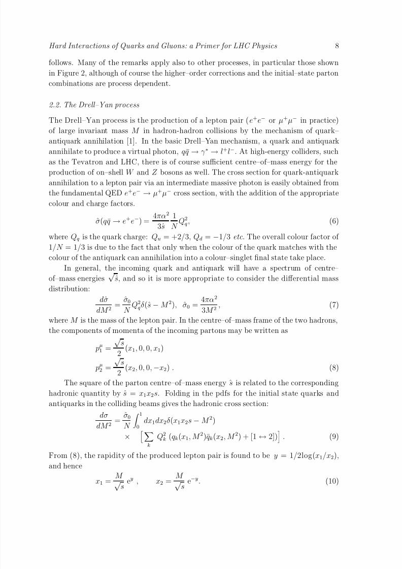
Figure 3. Graphical representation of the relationship between parton (x, Q2)
variables and the kinematic variables corresponding to a final state of mass M produced
with rapidity y at the LHC collider with√
s = 14 TeV.
The double–differential cross section is therefore
dσ
dM 2dy=
σ0
Ns
k
Q2k(qk(x1, M 2)qk(x2, M 2) + [1 ↔ 2])
. (11)
with x1 and x2 given by (10). Thus different values of M and y probe different values
of the parton x of the colliding beams. The formulae relating x1 and x2 to M and y
of course also apply to the production of any final state with this mass and rapidity.
Assuming the factorization scale (Q) is equal to M , the mass of the final state, the
relationship between the parton (x, Q2) values and the kinematic variables M and y is
illustrated pictorially in Figure 3, for the LHC collision energy √s = 14 TeV. For a
given rapidity y there are two (dashed) lines, corresponding to the values of x1 and x2.
For y = 0, x1 = x2 = M/√
s.
In analogy with the Drell–Yan cross section derived above, the subprocess cross
sections for (on–shell) W and Z production are readily calculated to be
σqq′→W =π
3
√2GF M 2W |V qq′|2δ(s − M 2W ),
σqq→Z =π
3
√2GF M 2Z (v2
q + a2q)δ(s − M 2Z ), (12)

8/3/2019 Hard Interactions of Quarks and Gluons a Primer for LHC Physics
http://slidepdf.com/reader/full/hard-interactions-of-quarks-and-gluons-a-primer-for-lhc-physics 10/118
Hard Interactions of Quarks and Gluons: a Primer for LHC Physics 10
Figure 4. Predictions for the W and Z total cross sections at the Tevatron and LHC,
using MRST2004 [10] and CTEQ6.1 pdfs [11], compared with recent data from CDF
and D0. The MRST predictions are shown at LO, NLO and NNLO. The CTEQ6.1
NLO predictions and the accompanying pdf error bands are also shown.
where V qq ′ is the appropriate Cabibbo–Kobayashi–Maskawa matrix element, and vq (aq)
is the vector (axial vector) coupling of the Z to the quarks. These formulae are valid in
the narrow width production in which the decay width of the gauge boson is neglected.
The resulting cross sections can then be multiplied by the branching ratio for any
particular hadronic or leptonic final state of interest.
High-precision measurements of W and Z production cross sections from the
Fermilab Tevatron p¯ p collider are available and allow the above formalism to be tested
quantitatively. Thus Figure 4 shows the cross sections for W ± and Z 0 production and
decay into various leptonic final states from the CDF [12] and D0 [13] collaborationsat the Tevatron. The theoretical predictions are calculated at LO (i.e. using (12)),
NLO and NNLO (next-to-next-to-leading order) in perturbation theory using the MS
scheme MRST parton distributions of [10], with renormalization and factorization scales
µF = µR = M W , M Z . The net effect of the NLO and NNLO corrections, which will be
discussed in more detail in Sections 3.3 and 3.4, is to increase the lowest-order cross
section by about 25% and 5% respectively.
Perhaps the most important point to note from Figure 4 is that, aside from unknown
(and presumably small) O(α3S ) corrections, there is virtually no theoretical uncertainty
associated with the predictions – the parton distributions are being probed in a range of x ∼ M W /√s where they are constrained from deep inelastic scattering, see Figure 3, and
the scale dependence is weak [10]. This overall agreement with experiment, therefore,
provides a powerful test of the whole theoretical edifice that goes into the calculation.
Figure 4 also illustrates the importance of higher-order perturbative corrections when
making detailed comparisons of data and theory.
8/3/2019 Hard Interactions of Quarks and Gluons a Primer for LHC Physics
http://slidepdf.com/reader/full/hard-interactions-of-quarks-and-gluons-a-primer-for-lhc-physics 11/118
Hard Interactions of Quarks and Gluons: a Primer for LHC Physics 11
p1
p2
p1
p2
Q
Q
Q
Q
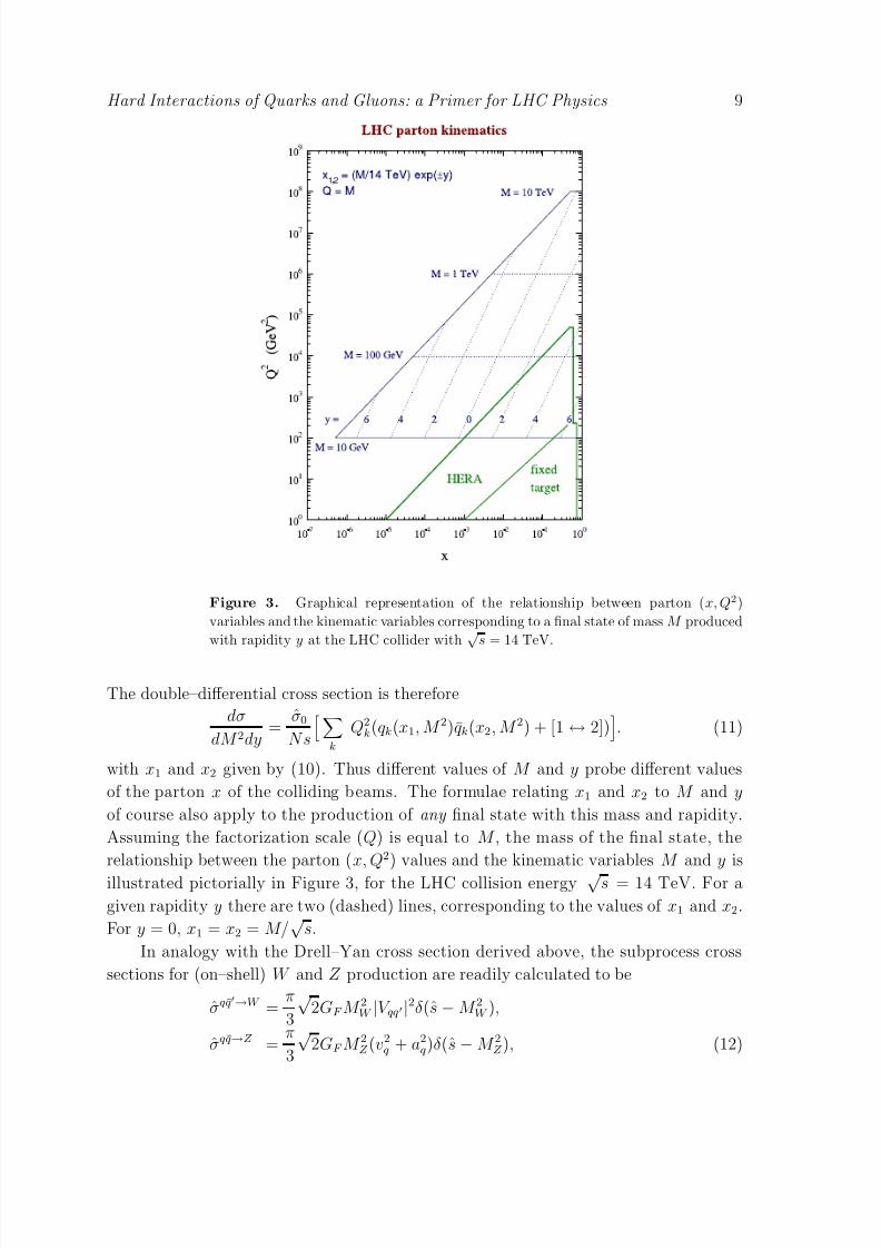
Figure 5. Representative Feynman diagrams for the production of a pair of heavy
quarks at hadron colliders, via gg (left) and qq (right) initial states.
2.3. Heavy quark production
The production of heavy quarks at hadron colliders proceeds via Feynman diagrams
such as the ones shown in Figure 5. Therefore, unlike the Drell-Yan process that we
have just discussed, in this case the cross section is sensitive to the gluon content of the incoming hadrons as well as the valence and sea quark distributions. The pdfs are
probed at values of x1 and x2 given by (c.f. equation (10)),
x1 =mT √
s(eyQ + eyQ) and x2 =
mT √s
e−yQ + e−yQ
, (13)
where mT is the transverse mass given by mT =
m2Q + p2
T , pT is the transverse
momentum of the quarks and yQ, yQ are the quark and antiquark rapidities. Although
more complicated than in the Drell-Yan case, these relations may be simply derived
using the same frame and notation as in (8) and writing, for instance, the 4-momentum
of the outgoing heavy quark as,
pµQ = (mT cosh yQ, pT , mT sinh yQ) , (14)
where pT is the 2-component transverse momentum. From examining (13) it is clear that
the dependence on the quark and gluon pdfs can vary considerably at different colliders
(√
s) and when producing different flavours of heavy quark (for instance, mc ≈ 1.5 GeV
compared to mt ≈ 175 GeV).
In this frame the heavy quark propagator that appears in the left-hand diagram of
Figure 5 can easily be evaluated. It is given by,
( pQ − p1)2 − m2Q = −2 pQ · p1 = −√
s x1mT (cosh yQ − sinh yQ) , (15)
which, when inserting the expression for x1 in (13) reduces to the simple relation,
( pQ − p1)2 − m2Q = −m2
T
1 + e(yQ−yQ)
. (16)
Thus the propagator always remains off-shell, since m2T ≥ m2
Q. This is in fact true for all
the propagators that appear in the diagrams for heavy quark production. The addition
of the mass scale mQ sets a lower bound for the propagators – which would not occur if
we considered the production of massless (or light) quarks, where the appropriate cut-off
would be the scale ΛQCD. Since the calculation would then enter the non-perturbative
domain, such processes cannot be calculated in the same way as for heavy quarks;
instead one must introduce a separate hard scale to render the calculation perturbative,

8/3/2019 Hard Interactions of Quarks and Gluons a Primer for LHC Physics
http://slidepdf.com/reader/full/hard-interactions-of-quarks-and-gluons-a-primer-for-lhc-physics 12/118
Hard Interactions of Quarks and Gluons: a Primer for LHC Physics 12
t
Figure 6. The one-loop diagram representing Higgs production via gluon fusion at
hadron colliders. The dominant contribution is from a top quark circulating in the
loop, as illustrated.
as we shall discuss at more length in Section 3.2. In contrast, as long as the quark is
sufficiently heavy, mQ ≫ ΛQCD (as is certainly the case for top and bottom quarks), themass sets a scale at which perturbation theory is expected to hold.
Although we shall not concentrate on the many aspects of heavy quark processes
in this article, we will examine the success of perturbation theory for the case of top
production at the Tevatron in Section 5.5.
2.4. Higgs boson production
The search for the elusive Higgs boson has been the focus of much analysis at both
the Tevatron and the LHC. As such, many different channels have been proposed in
which to observe events containing Higgs bosons, including the production of a Higgs
boson in association with a W or a Z as well as Higgs production with a pair of heavy
quarks. However, the largest rate for a putative Higgs boson at both the Tevatron and
the LHC results from the gluon fusion process depicted in Figure 6. Since the Higgs
boson is responsible for giving mass to the particles in the Standard Model, it couples
to fermions with a strength proportional to the fermion mass. Therefore, although any
quark may circulate in the loop, the largest contribution by far results from the top
quark. Since the LO diagram already contains a loop, the production of a Higgs boson
in this way is considerably harder to calculate than the tree level processes mentioned
thus far – particularly when one starts to consider higher orders in perturbation theory
or the radiation of additional hard jets.For this reason it is convenient to formulate the diagram in Figure 6 as an effective
coupling of the Higgs boson to two gluons in the limit that the top quark is infinitely
massive. Although formally one would expect that this approximation is valid only
when all other scales in the problem are much smaller than mt, in fact one finds that
only mH < mt (and pT (jet) < mt, when additional jets are present) is necessary for an
accurate approximation [3]. Using this approach the Higgs boson cross section via gluon
fusion has been calculated to NNLO [4, 5], as we shall discuss further in Section 3.4.
The second-largest Higgs boson cross section at the LHC is provided by the weak-
boson fusion (WBF) mechanism, which proceeds via the exchange of W or Z bosons

8/3/2019 Hard Interactions of Quarks and Gluons a Primer for LHC Physics
http://slidepdf.com/reader/full/hard-interactions-of-quarks-and-gluons-a-primer-for-lhc-physics 13/118
Hard Interactions of Quarks and Gluons: a Primer for LHC Physics 13
q
q
q
q
W
W H
q
q
q
q
Z
Z H
Figure 7. Diagrams representing the production of a Higgs boson via the weak boson
fusion mechanism.
from incoming quarks, as shown in Figure 7. Although this process is an electroweak one
and therefore proceeds at a slower rate (about an order of magnitude lower than gluon
fusion) it has a very clear experimental signature. The incoming quarks only receive
a very small kick in their direction when radiating the W or Z bosons, so they can in
principle be detected as jets very forward and backward at large absolute rapidities. At
the same time, since no coloured particles are exchanged between the quark lines, very
little hadronic radiation is expected in the central region of the detector. Therefore the
type of event that is expected from this mechanism is often characterized by a “rapidity
gap” in the hadronic calorimeters of the experiment. As well as forming part of the
search strategy for the Higgs boson, this channel opens up the possibility of measuring
the nature of the Higgs coupling to vector bosons [6].
Although the scope of this review does not allow a lengthy discussion of the manyfacets of Higgs physics, including all its production mechanisms, decay modes, search
strategies and properties, we will touch on a few important aspects of Higgs boson
phenomenology, particularly in Section 2.4. For a recent and more complete review of
Higgs physics we refer the reader to [7].
2.5. W and Z transverse momentum distributions
Like Drell-Yan lepton pairs, most W and Z bosons (here collectively denoted by V ) are
produced with relatively little transverse momentum, i.e. pT ≪ M V . In the leading-
order model discussed in Section 2.2, in which the colliding partons are assumed tobe exactly collinear with the colliding beam particles, the gauge bosons are produced
with zero transverse momentum. This approach does not take account of the intrinsic
(non-perturbative) transverse motion of the quarks and gluons inside the colliding
hadrons, nor of the possibility of generating large transverse momentum by recoil against
additional energetic partons produced in the hard scattering.
At very small pT , the intrinsic transverse motion of the quarks and gluons inside the
colliding hadrons, kT ∼ ΛQCD, cannot be neglected. Indeed the measured pT distribution
of Drell–Yan lepton pairs produced in fixed-target pN collisions is well parametrized
by assuming a Gaussian distribution for the intrinsic transverse momentum with

8/3/2019 Hard Interactions of Quarks and Gluons a Primer for LHC Physics
http://slidepdf.com/reader/full/hard-interactions-of-quarks-and-gluons-a-primer-for-lhc-physics 14/118
Hard Interactions of Quarks and Gluons: a Primer for LHC Physics 14
kT ∼ 700 MeV, see for example [8]. However the data on the pT distribution also
show clear evidence of a hard, power-law tail, and it is natural to attribute this to the
(perturbative) emission of one or more hard partons, i.e. qq → V g, qg → V q etc. The
Feynman diagrams for these processes are identical to those for large pT direct photon
production, and the corresponding annihilation and Compton matrix elements are, for
W production,
|Mqq′→Wg|2 = παS
√2GF M 2W |V qq′|2 8
9
t2 + u2 + 2M 2W s
tu,
|Mgq→Wq′|2 = παS
√2GF M 2W |V qq′|2 1
3
s2 + u2 + 2tM 2W
−su, (17)
with similar results for the Z boson and for Drell–Yan lepton pairs. The sum is over
colours and spins in the final and initial states, with appropriate averaging factors for the
latter. The transverse momentum distribution dσ/dp2T is then obtained by convoluting
these matrix elements with parton distributions in the usual way. In principle, onecan combine the hard (perturbative) and intrinsic (non-perturbative) contributions, for
example using a convolution integral in transverse momentum space, to give a theoretical
prediction valid for all pT . A more refined prediction would then include next-to-leading-
order (O(α2S )) perturbative corrections, for example from processes like qq → V gg , to
the high pT tail. Some fraction of the O(αS ) and O(α2S ) contributions could be expected
to correspond to distinct V + 1 jet and V + 2 jet final states respectively.
However, a major problem in carrying out the above procedure is that the 2 → 2
matrix elements are singular when the final-state partons become soft and/or are emitted
collinear with the initial-state partons. These singularities are related to the poles at
t = 0 and u = 0 in the above matrix elements. In addition, processes like qq → V gg are
singular when the two final-state gluons become collinear. This means in practice that
the lowest-order perturbative contribution to the pT distribution is singular as pT → 0,
and that higher-order contributions from processes like qq → V gg are singular for any
pT .
The fact that the predictions of perturbative QCD are in fact finite for physical
processes is due to a number of deep and powerful theorems (applicable to any quantum
field theory) that guarantee that for suitably defined cross sections and distributions,
the singularities arising from real and virtual parton emissions at intermediate stages
of the calculation cancel when all contributions are included. We have already seen anexample of this in the discussion above. The O(αS ) contribution to the total W cross
section from the process qq → W g is singular when pT (W ) = 0, but this singularity
is exactly cancelled by a O(αS ) contribution from a virtual gluon loop correction to
qq → W . The net result is the finite NLO contribution to the cross section displayed
in Figure 4. The details of how and under what circumstances these cancellations take
place will be discussed in the following section.
8/3/2019 Hard Interactions of Quarks and Gluons a Primer for LHC Physics
http://slidepdf.com/reader/full/hard-interactions-of-quarks-and-gluons-a-primer-for-lhc-physics 15/118
Hard Interactions of Quarks and Gluons: a Primer for LHC Physics 15
W +
u
d
W +
u
d
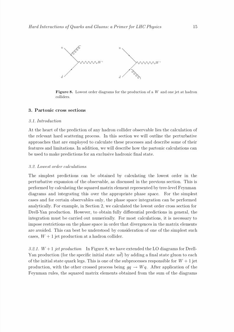
Figure 8. Lowest order diagrams for the production of a W and one jet at hadron
colliders.
3. Partonic cross sections
3.1. Introduction
At the heart of the prediction of any hadron collider observable lies the calculation of
the relevant hard scattering process. In this section we will outline the perturbative
approaches that are employed to calculate these processes and describe some of their
features and limitations. In addition, we will describe how the partonic calculations can
be used to make predictions for an exclusive hadronic final state.
3.2. Lowest order calculations
The simplest predictions can be obtained by calculating the lowest order in theperturbative expansion of the observable, as discussed in the previous section. This is
performed by calculating the squared matrix element represented by tree-level Feynman
diagrams and integrating this over the appropriate phase space. For the simplest
cases and for certain observables only, the phase space integration can be performed
analytically. For example, in Section 2, we calculated the lowest order cross section for
Drell-Yan production. However, to obtain fully differential predictions in general, the
integration must be carried out numerically. For most calculations, it is necessary to
impose restrictions on the phase space in order that divergences in the matrix elements
are avoided. This can best be understood by consideration of one of the simplest suchcases, W + 1 jet production at a hadron collider.
3.2.1. W + 1 jet production In Figure 8, we have extended the LO diagrams for Drell-
Yan production (for the specific initial state ud) by adding a final state gluon to each
of the initial state quark legs. This is one of the subprocesses responsible for W + 1 jet
production, with the other crossed process being gq → W q. After application of the
Feynman rules, the squared matrix elements obtained from the sum of the diagrams

8/3/2019 Hard Interactions of Quarks and Gluons a Primer for LHC Physics
http://slidepdf.com/reader/full/hard-interactions-of-quarks-and-gluons-a-primer-for-lhc-physics 16/118
Hard Interactions of Quarks and Gluons: a Primer for LHC Physics 16
take the form:
|Mud→W +g|2 ∼
t2 + u2 + 2Q2 s
tu
, (18)
where Q2
is the virtuality of the W boson, s = sud, t = sug, and u = sdg , c.f. (17) of Section 2. This expression diverges in the limit where the gluon is unresolved – either it
is collinear to one of the quarks (t → 0 or u → 0), or it is soft (both invariants vanish, so
E g → 0). Let us consider the impact of these divergences on the calculation of this cross
section. In order to turn the matrix elements into a cross section, one must convolute
with pdfs and perform the integration over the appropriate phase space,
σ =
dx1dx2f u(x1, Q2)f d(x2, Q2)|M|232π2s
d3 pW
E W
d3 pg
E gδ( pu + pd − pg − pW ), (19)
where x1, x2 are the momentum fractions of the u and d quarks. These momentum
fractions are of course related to the centre-of-mass energy squared of the collider s by
the relation, s = x1x2s.
After suitable manipulations, this can be transformed into a cross section that
is differential in Q2 and the transverse momentum ( pT ) and rapidity (y) of the W
boson [39],
dσ
dQ2dydp2T ∼ 1
s
dyg f u(x1, Q2)f d(x2, Q2)
|M|2s
(20)
The remaining integral to be done is over the rapidity of the gluon, yg. Note that the pT
of the gluon is related to the invariants of the process by p2T = tu/s. Thus the leading
divergence represented by the third term of (18), where t and u both approach zero and
the gluon is soft, can be written as 1/p2T . Furthermore, in this limit s → Q2, so thatthe behaviour of the cross section becomes,
dσ
dQ2dydp2T
∼ 2
s
1
p2T
dyg f u(x1, Q2)f d(x2, Q2) + (sub-leading in p2T ) . (21)
As the pT of the W boson becomes small, the limits on the yg integration are given by
± log(√
s/pT ). Under the assumption that the rest of the integrand is approximately
constant, the integral can be simply performed. This yields,
dσ
dQ2dydp2T ∼ log(s/p2T )
p2T , (22)
so that the differential cross section contains a logarithmic dependence on pT . If no cutis applied on the gluon pT then the integral over pT diverges – only after applying
a minimum value of the pT do we obtain a finite result. Once we apply a cutoff
at pT = pT,min and then perform the integration, we find a result proportional to
log2(s/p2T,min). This is typical of a fixed order expansion – it is not merely an expansion
in αS , but in αS log(. . .), where the argument of the logarithm depends upon the process
and cuts under consideration. As we shall discuss later, these logarithms may be
systematically accounted for in various all-orders treatments.
In Figure 9 we show the rapidity distribution of the jet, calculated using this lowest
order process. In the calculation, a sum over all species of quarks has been performed

8/3/2019 Hard Interactions of Quarks and Gluons a Primer for LHC Physics
http://slidepdf.com/reader/full/hard-interactions-of-quarks-and-gluons-a-primer-for-lhc-physics 17/118
Hard Interactions of Quarks and Gluons: a Primer for LHC Physics 17
Figure 9. The rapidity distribution of the final state parton found in a lowest order
calculation of the W + 1 jet cross section at the LHC. The parton is required to have
a pT larger than 2 GeV (left) or 50 GeV(right). Contributions from qq annihilation
(solid red line) and the qg process (dashed blue line) are shown separately.
u
d
u
dW +
W +
Figure 10. An alternative way of drawing the diagrams of Figure 8.
and the contribution from the quark-gluon process included. The rapidity distribution
is shown for two different choices of minimum jet transverse momentum, which is the
cut-off used to regulate the collinear divergences discussed above. For very small values
of pT , we can view the radiated gluon as being emitted from the quark line at an early
time, typically termed “initial-state radiation”. From the left-hand plot, this radiation is
indeed produced quite often at large rapidities, although it is also emitted centrally with
a large probability. The canonical “wisdom” is that initial-state radiation is primarily
found in the forward region. There is indeed a collinear pole in the matrix element
so that a fixed energy gluon tends to be emitted close to the original parton direction.However, we are interested not in fixed energy but rather in fixed transverse momentum.
When using a higher pT cut-off the gluon is emitted less often at large rapidities and is
more central, as shown by the plot on the right-hand side. In this case, one can instead
think of the diagrams as a 2 → 2 scattering as depicted in Figure 10. Of course, the
manner in which such Feynman diagrams are drawn is purely a matter of convention.
The diagrams are exactly the same as in Figure 8, but re-drawing them in this way is
suggestive of the different kinematic region that is probed with a gluon at high pT .
There is also a collinear pole involved for the emission of gluons from final state
partons. Thus, the gluons will be emitted preferentially near the direction of the emitting

8/3/2019 Hard Interactions of Quarks and Gluons a Primer for LHC Physics
http://slidepdf.com/reader/full/hard-interactions-of-quarks-and-gluons-a-primer-for-lhc-physics 18/118
Hard Interactions of Quarks and Gluons: a Primer for LHC Physics 18
Figure 11. The 4 diagrams that contribute to the matrix elements for the production
of W + 2 gluons when gluon 1 is soft.
parton. In fact, it is just such emissions that give rise to the finite size of the jet arising
from a single final state parton originating from the hard scatter. Much of the jet
structure is determined by the hardest gluon emission; thus NLO theory, in which a jet
consists of at most 2 partons, provides a good description of the jet shape observed in
data [14].
3.2.2. W + 2 jet production By adding a further parton, one can simulate the
production of a W + 2 jet final state. Many different partonic processes contribute
in general, so for the sake of illustration we just consider the production of a W boson
in association with two gluons.
First, we shall study the singularity structure of the matrix elements in more detail.
In the limit that one of the gluons, p1, is soft the singularities in the matrix elements
occur in 4 diagrams only. These diagrams, in which gluon p1 is radiated from an external
line, are depicted in Figure 11. The remaining diagrams, in which gluon p1 is attached
to an internal line, do not give rise to singularities because the adjacent propagator doesnot vanish in this limit.
This is the first of our examples in which the matrix elements contain non-trivial
colour structure. Denoting the colour labels of gluons p1 and p2 by tA and tB respectively,
diagram (1) is proportional to tBtA, whilst (2) is proportional to tAtB. The final two
diagrams, (3a) and (3b) are each proportional to f ABC tC , which can of course be written
as (tAtB − tBtA). Using this identity, the amplitude (in the limit that p1 is soft) can be
written in a form in which the dependence on the colour matrices is factored out,
Mqq→Wgg = tAtB(D2 + D3) + tBtA(D1 − D3) (23)

8/3/2019 Hard Interactions of Quarks and Gluons a Primer for LHC Physics
http://slidepdf.com/reader/full/hard-interactions-of-quarks-and-gluons-a-primer-for-lhc-physics 19/118
Hard Interactions of Quarks and Gluons: a Primer for LHC Physics 19
so that the kinematic structures obtained from the Feynman rules are collected in the
functions D1, D2 (for diagrams (1) and (2)) and D3 (the sum of diagrams (3a) and (3b)).
The combinations of these that appear in (23) are often referred to as colour-ordered
amplitudes.
With the colour factors stripped out, it is straightforward to square the amplitude
in (23) using the identities tr(tAtBtBtA) = NC 2F and tr(tAtBtAtB) = −C F /2,
|Mqq→Wgg|2 = NC 2F |D2 + D3|2 + |D1 − D3|2
− C F Re[(D2 + D3)(D1 − D3)⋆]
=C F N 2
2
|D2 + D3|2 + |D1 − D3|2 − 1
N 2|D1 + D2|2
. (24)
Moreover, these colour-ordered amplitudes possess special factorization properties in
the limit that gluon p1 is soft. They can be written as the product of an eikonal term
and the matrix elements containing only one gluon,
D2 + D3 −→ ǫµ
qµ
p1.q − p
µ
2 p1.p2
Mqq→Wg
D1 − D3 −→ ǫµ
pµ2
p1.p2− qµ
p1.q
Mqq→Wg (25)
where ǫµ is the polarization vector for gluon p1. The squares of these eikonal terms are
easily computed using the replacement ǫµǫ⋆ν → −gµν to sum over the gluon polarizations.
This yields terms of the form,
a.b
p1.a p1.b≡ [a b], (26)
so that the final result is,
|Mqq→Wgg|2 soft−→ C F N 2
2
[q p2] + [ p2 q] − 1
N 2[q q]
Mqq→Wg. (27)
Inspecting this equation, one can see that the leading term (in the number of colours)
contains singularities along two lines of colour flow – one connecting the gluon p2 to the
quark, the other connecting it to the antiquark. On the other hand, the sub-leading
term has singularities along the line connecting the quark and antiquark. It is these
lines of colour flow that indicate the preferred directions for the emission of additional
gluons. In the sub-leading term the colour flow does not relate the gluon colour to the
parent quarks at all. The matrix elements are in fact the same as those for the emission
of two photons from a quark line (apart from overall coupling factors) with no unique
assignment to either diagram 1 or diagram 2, unlike the leading term. For this reason
only the information about the leading colour flow is used by parton shower Monte
Carlos such as HERWIG [15] and PYTHIA [16]. These lines of colour flow generalize in
an obvious manner to higher multiplicity final states. As as example, the lines of colour
flow in a W + 2 jet event are shown in Figure 12.
Since all the partons are massless, it is trivial to re-write the eikonal factor of (26)
in terms of the energy of the radiated gluon, E and the angle it makes with the hard

8/3/2019 Hard Interactions of Quarks and Gluons a Primer for LHC Physics
http://slidepdf.com/reader/full/hard-interactions-of-quarks-and-gluons-a-primer-for-lhc-physics 20/118
Hard Interactions of Quarks and Gluons: a Primer for LHC Physics 20
W
1
2
q
q W
1
2
q
q
Figure 12. Two examples of colour flow in a W + 2 jet event, shown in red. In the
left hand diagram, a leading colour flow is shown. The right-hand diagram depicts the
sub-leading colour flow resulting from interference.
partons, θa, θb. It can then be combined with the phase space for the emitted gluon to
yield a contribution such as,
[a b] dP S gluon =
1
E 2
1
1 − cos θa EdE d cos θa . (28)
In this form, it is clear that the cross section diverges as either cos θa → 1 (the gluon
is emitted collinear to parton a) or E → 0 (for any angle of radiation). Moreover,
each divergence is logarithmic and regulating the divergence, by providing a fixed cutoff
(either in angle or energy), will produce a single logarithm from collinear configurations
and another from soft ones – just as we found when considering the specific case of
W + 1 jet production in the previous subsection.
This argument can be applied at successively higher orders of perturbation theory.
Each gluon that is added yields an additional power of αS and, via the eikonal
factorization outlined above, can produce an additional two logarithms. This meansthat we can write the W + 1 jet cross section schematically as a sum of contributions,
dσ = σ0(W + 1 jet)1 + αS (c12L2 + c11L + c10)
+α2S (c24L4 + c23L3 + c22L2 + c21L + c20) + . . .
(29)
where L represents the logarithm controlling the divergence, either soft or collinear. The
size of L depends upon the criteria used to define the jets – the minimum transverse
energy of a jet and the jet cone size. The coefficients cij in front of the logarithms
depend upon colour factors. Note that the addition of each gluon results not just in
an additional factor of αS , but in a factor of αS times logarithms. For many important
kinematic configurations, the logs can be large, leading to an enhanced probability foradditional gluon emissions to occur. For inclusive quantities, where the same cuts are
applied to every jet, the logs tends to be small, and counting powers of αS becomes a
valid estimator for the rate of production of additional jets.
Noticing that the factor (αS L) appears throughout (29), it is useful to re-write the
expansion in brackets as,. . .
= 1 + αS L
2c12 + (αS L2)2c24 + αS Lc11(1 + αS L
2c23/c11 + . . .) + . . .
= expc12αS L
2 + c11αS L
, (30)

8/3/2019 Hard Interactions of Quarks and Gluons a Primer for LHC Physics
http://slidepdf.com/reader/full/hard-interactions-of-quarks-and-gluons-a-primer-for-lhc-physics 21/118
Hard Interactions of Quarks and Gluons: a Primer for LHC Physics 21
where the infinite series have been resummed into an exponential form†. The first term in
the exponent is commonly referred to as the leading logarithmic term, with the second
being required in order to reproduce next-to-leading logarithms. This reorganization
of the perturbative expansion is especially useful when the product αS L is large, for
instance when the logarithm is a ratio of two physical scales that are very different such
as log(mH /mb). This exponential form is the basis of all orders predictions and can be
interpreted in terms of Sudakov probabilities, both subjects that we will return to in
later discussions.
It is instructive to recast the discussion of the total W cross section in these terms,
where the calculation is decomposed into components that each contain a given number
of jets:
σW = σW +0 j + σW +1 j + σW +2 j + σW +3 j + . . . (31)
Now, as in (29), we can further write out each contribution as an expansion in powersof αS and logarithms,
σW +0 j = a0 + αS (a12L2 + a11L + a10)
+ α2S (a24L4 + a23L3 + a22L2 + a21L + a20) + . . .
σW +1 j = αS (b12L2 + b11L + b10)
+ α2S (b24L4 + b23L3 + b22L2 + b21L + b20) + . . .
σW +2 j = . . . . (32)
As the jet definitions change, the size of the logarithms shuffle the contributions from
one jet cross section to another, whilst keeping the sum over all jet contributions the
same. For example, as the jet cone size is decreased the logarithm L increases. As a
result, the average jet multiplicity goes up and terms in (31) that represent relatively
higher multiplicities will become more important.
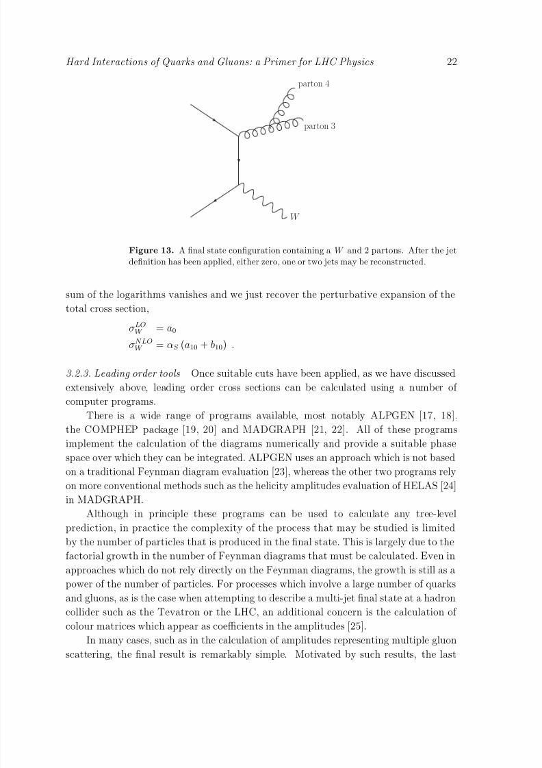
This is illustrated in Figure 13. Such a configuration may be reconstructed as an
event containing up to two jets, depending upon the jet definition and the momenta
of the partons. The matrix elements for this process contain terms proportional to
αS log( pT,3/pT,4) and αS log(1/∆R34) which is the reason that minimum values for the
transverse energy and separation must be imposed. We shall see later that this is not the
case in a full next-to-leading order calculation where these soft and collinear divergences
are cancelled.Finally, we note that although the decomposition in (31) introduces quantities
which are dependent upon the jet definition, we can recover results that are independent
of these parameters by simply summing up the terms in the expansion that enter at the
same order of perturbation theory, i.e. the aij and bij in equation 32 are not independent.
As we will discuss shortly, in Section 3.3, at a given order of perturbation theory the
† Unfortunately, systematically collecting the terms in this way is far from trivial and only possible
when considering certain observables and under specific choices of jet definition (such as when using
the kT -clustering algorithm).
8/3/2019 Hard Interactions of Quarks and Gluons a Primer for LHC Physics
http://slidepdf.com/reader/full/hard-interactions-of-quarks-and-gluons-a-primer-for-lhc-physics 22/118
Hard Interactions of Quarks and Gluons: a Primer for LHC Physics 22
W
parton 3
parton 4
Figure 13. A final state configuration containing a W and 2 partons. After the jet
definition has been applied, either zero, one or two jets may be reconstructed.
sum of the logarithms vanishes and we just recover the perturbative expansion of the
total cross section,
σLOW = a0
σNLOW = αS (a10 + b10) .
3.2.3. Leading order tools Once suitable cuts have been applied, as we have discussed
extensively above, leading order cross sections can be calculated using a number of
computer programs.There is a wide range of programs available, most notably ALPGEN [17, 18],
the COMPHEP package [19, 20] and MADGRAPH [21, 22]. All of these programs
implement the calculation of the diagrams numerically and provide a suitable phase
space over which they can be integrated. ALPGEN uses an approach which is not based
on a traditional Feynman diagram evaluation [23], whereas the other two programs rely
on more conventional methods such as the helicity amplitudes evaluation of HELAS [24]
in MADGRAPH.
Although in principle these programs can be used to calculate any tree-level
prediction, in practice the complexity of the process that may be studied is limited
by the number of particles that is produced in the final state. This is largely due to thefactorial growth in the number of Feynman diagrams that must be calculated. Even in
approaches which do not rely directly on the Feynman diagrams, the growth is still as a
power of the number of particles. For processes which involve a large number of quarks
and gluons, as is the case when attempting to describe a multi-jet final state at a hadron
collider such as the Tevatron or the LHC, an additional concern is the calculation of
colour matrices which appear as coefficients in the amplitudes [25].
In many cases, such as in the calculation of amplitudes representing multiple gluon
scattering, the final result is remarkably simple. Motivated by such results, the last
8/3/2019 Hard Interactions of Quarks and Gluons a Primer for LHC Physics
http://slidepdf.com/reader/full/hard-interactions-of-quarks-and-gluons-a-primer-for-lhc-physics 23/118
Hard Interactions of Quarks and Gluons: a Primer for LHC Physics 23
couple of years has seen remarkable progress in the development of new approaches
to QCD tree-level calculations. Some of the structure behind the amplitudes can be
understood by transforming to “twistor space” [26], in which amplitudes are represented
by intersecting lines. This idea can be taken further with the introduction of “MHV”
rules [27], which use the simplest (maximally helicity-violating, or MHV) amplitudes
as the building blocks of more complicated ones. Although these rules at first only
applied to amplitudes containing gluons, they were soon extended to cases of more
general interest at hadron colliders [28, 29, 30, 31, 32, 33]. Even more recently,
further simplification of amplitudes has been obtained by using “on-shell recursion
relations” [34, 35]. As well as providing very compact expressions, this approach has
the advantage of being both easily proven and readily extendible to processes involving
fermions and vector bosons.
3.3. Next-to-leading order calculations
Although lowest order calculations can in general describe broad features of a particular
process and provide the first estimate of its cross section, in many cases this
approximation is insufficient. The inherent uncertainty in a lowest order calculation
derives from its dependence on the unphysical renormalization and factorization scales,
which is often large. In addition, some processes may contain large logarithms that
need to be resummed or extra partonic processes may contribute only when going
beyond the first approximation. Thus, in order to compare with predictions that have
smaller theoretical uncertainties, next-to-leading order calculations are imperative for
experimental analyses in Run II of the Tevatron and at the LHC.
3.3.1. Virtual and real radiation A next-to-leading order QCD calculation requires the
consideration of all diagrams that contribute an additional strong coupling factor, αS .
These diagrams are obtained from the lowest order ones by adding additional quarks and
gluons and they can be divided into two categories, virtual (or loop) contributions and
the real radiation component. We shall illustrate this by considering the next-to-leading
order corrections to Drell-Yan production at a hadron collider. The virtual diagrams
for this process are shown in Figure 14 whilst the real diagrams are exactly the ones
that enter the W + 1 jet calculation (in Figure 8).
Let us first consider the virtual contributions. In order to evaluate the diagrams inFigure 14, it is necessary to introduce an additional loop momentum ℓ which circulates
around the loop in each diagram and is unconstrained. To complete the evaluation
of these diagrams, one must therefore integrate over the momentum ℓ. However, the
resulting contribution is not finite but contains infrared divergences – in the same way
that the diagrams of Figure 8 contain infrared (soft and collinear) singularities. By
isolating the singularities appropriately, one can see that the divergences that appear
in each contribution are equal, but of opposite sign. The fact that the sum is finite is
a demonstration of the theorems of Bloch and Nordsieck [36] and Kinoshita, Lee and

8/3/2019 Hard Interactions of Quarks and Gluons a Primer for LHC Physics
http://slidepdf.com/reader/full/hard-interactions-of-quarks-and-gluons-a-primer-for-lhc-physics 24/118
Hard Interactions of Quarks and Gluons: a Primer for LHC Physics 24
W +
u
d
W +
u
d
W +
u
d
Figure 14. Virtual diagrams included in the next-to-leading order corrections to
Drell-Yan production of a W at hadron colliders.
Nauenberg [37, 38], which guarantee that this is the case at all orders in perturbation
theory and for any number of final state particles.
The real contribution consists of the diagrams in Figure 8, together with a quark-gluon scattering piece that can be obtained from these diagrams by interchanging the
gluon in the final state with a quark (or antiquark) in the initial state. As discussed in
Section 3.2.1, the quark-antiquark matrix elements contain a singularity as the gluon
transverse momentum vanishes.
In our NLO calculation we want to carefully regulate and then isolate these
singularities in order to extend the treatment down to zero transverse momentum. The
most common method to regulate the singularities is dimensional regularization. In this
approach the number of dimensions is continued to D = 4 − 2ǫ, where ǫ < 0, so that
in intermediate stages the singularities appear as single and double poles in ǫ. After
they have cancelled, the limit D → 4 can be safely taken. Within this scheme, thecancellation of divergences between real and virtual terms can be seen schematically by
consideration of a toy calculation [40],
I = limǫ→0
10
dx
xx−ǫM(x) +
1
ǫM(0)
. (33)
Here, M(x) represents the real radiation matrix elements which are integrated over
the extra phase space of the gluon emission, which contains a regulating factor x−ǫ. x
represents a kinematic invariant which vanishes as the gluon becomes unresolved. The
second term is representative of the virtual contribution, which contains an explicit pole,
1/ǫ, multiplying the lowest order matrix elements, M(0).Two main techniques have been developed for isolating the singularities, which
are commonly referred to as the subtraction method [41, 42, 43, 44] and phase-space
slicing [45, 46]. For the sake of illustration, we shall consider only the subtraction
method. In this approach, one explicitly adds and subtracts a divergent term such that
the new real radiation integral is manifestly finite. In the toy integral this corresponds
to,
I = limǫ→0
10
dx
xx−ǫ [M(x) − M(0)] + M(0)
10
dx
xx−ǫ +
1
ǫM(0)

8/3/2019 Hard Interactions of Quarks and Gluons a Primer for LHC Physics
http://slidepdf.com/reader/full/hard-interactions-of-quarks-and-gluons-a-primer-for-lhc-physics 25/118
Hard Interactions of Quarks and Gluons: a Primer for LHC Physics 25
u
u
u
u
Figure 15. The leading order diagrams representing inclusive jet production from a
quark antiquark initial state.
= 10
dx
x[M(x) − M(0)] . (34)
This idea can be generalized in order to render finite the real radiation contribution
to any process, with a separate counter-term for each singular region of phase space.Processes with a complicated phase space, such as W + 2 jet production, can end up
with a large number of counterterms. NLO calculations are often set up to generate
cross sections by histogramming “events” generated with the relevant matrix elements.
Such events can not be directly interfaced to parton shower programs, which we will
discuss later in Section 3.5, as the presence of virtual corrections means that many of
the events will have (often large) negative weights. Only the total sum of events over
all relevant subprocesses will lead to a physically meaningful cross section.
The inclusion of real radiation diagrams in a NLO calculation extends the range
of predictions that may be described by a lowest order calculation. For instance, in
the example above the W boson is produced with zero transverse momentum at lowest
order and only acquires a finite pT at NLO. Even then, the W transverse momentum
is exactly balanced by that of a single parton. In a real event, the W pT is typically
balanced by the sum of several jet transverse momenta. In a fixed order calculation,
these contributions would be included by moving to even higher orders so that, for
instance, configurations where the W transverse momentum is balanced by two jets
enter at NNLO. Although this feature is clear for the pT distribution of the W , the
same argument applies for other distributions and for more complex processes.
3.3.2. Scale dependence One of the benefits of performing a calculation to higherorder in perturbation theory is the reduction of the dependence of related predictions
on the unphysical renormalization (µR) and factorization scales (µF ). This can be
demonstrated by considering inclusive jet production from a quark antiquark initial
state [11], which is represented by the lowest order diagrams shown in Figure 15. This
is a simplification of the full calculation, but is the dominant contribution when the
typical jet transverse momentum is large.
For this process, we can write the lowest order prediction for the single jet inclusive

8/3/2019 Hard Interactions of Quarks and Gluons a Primer for LHC Physics
http://slidepdf.com/reader/full/hard-interactions-of-quarks-and-gluons-a-primer-for-lhc-physics 26/118
Hard Interactions of Quarks and Gluons: a Primer for LHC Physics 26
distribution as,
dσ
dE T = α2
S (µR) σ0 ⊗ f q(µF ) ⊗ f q(µF ), (35)
where σ0 represents the lowest order partonic cross section calculated from the diagramsof Figure 15 and f i(µF ) is the parton distribution function for a parton i. Similarly,
after including the next-to-leading order corrections, the prediction can be written as,
dσ
dE T =
α2S (µR)σ0 + α3
S (µR)
σ1 + 2b0 log(µR/E T )σ0 − 2P qq log(µF /E T )σ0
⊗f q(µF ) ⊗ f q(µF ). (36)
In this expression the logarithms that explicitly involve the renormalization and
factorization scales have been exposed. The remainder of the O(α3S ) corrections lie
in the function σ1.
From this expression, the sensitivity of the distribution to the renormalization scaleis easily calculated using,
µR∂αS (µR)
∂µR= −b0α2
S (µR) − b1α3S (µR) + O(α4
S ), (37)
where the two leading coefficients in the beta-function, b0 and b1, are given by
b0 = (33 − 2nf )/6π, b1 = (102 − 38nf /3)/8π2. The contributions from the first and
third terms in (36) cancel and the result vanishes, up to O(α4S ) .
In a similar fashion, the factorization scale dependence can be calculated using the
non-singlet DGLAP equation,
µF ∂f i(µF )
∂µF = αS (µF )P qq ⊗ f i(µF ). (38)
This time, the partial derivative of each parton distribution function, multiplied by the
first term in (36), cancels with the final term. Thus, once again, the only remaining
terms are of order α4S .
This is a generic feature of a next-to-leading order calculation. An observable
that is predicted to order αnS is independent of the choice of either renormalization or
factorization scale, up to the next higher order in αS .
This discussion can be made more concrete by inserting numerical results into the
formulae indicated above. For simplicity, we will consider only the renormalization scale
dependence, with the factorization scale held fixed at µF = E T . In this case it is simpleto extend (36) one higher order in αS [51],
dσ
dE T =
α2S (µR) σ0 + α3
S (µR)
σ1 + 2b0L σ0
+α4S (µR)
σ2 + 3b0L σ1 + (3b20L2 + 2b1L) σ0
⊗ f q(µF ) ⊗ f q(µF ), (39)
where the logarithm is abbreviated as L ≡ log(µR/E T ). For a realistic example at the
Tevatron Run I, σ0 = 24.4 and σ1 = 101.5. With these values the LO and NLO scale
dependence can be calculated; the result is shown in Figure 16, adapted from [51]. At
8/3/2019 Hard Interactions of Quarks and Gluons a Primer for LHC Physics
http://slidepdf.com/reader/full/hard-interactions-of-quarks-and-gluons-a-primer-for-lhc-physics 27/118
Hard Interactions of Quarks and Gluons: a Primer for LHC Physics 27
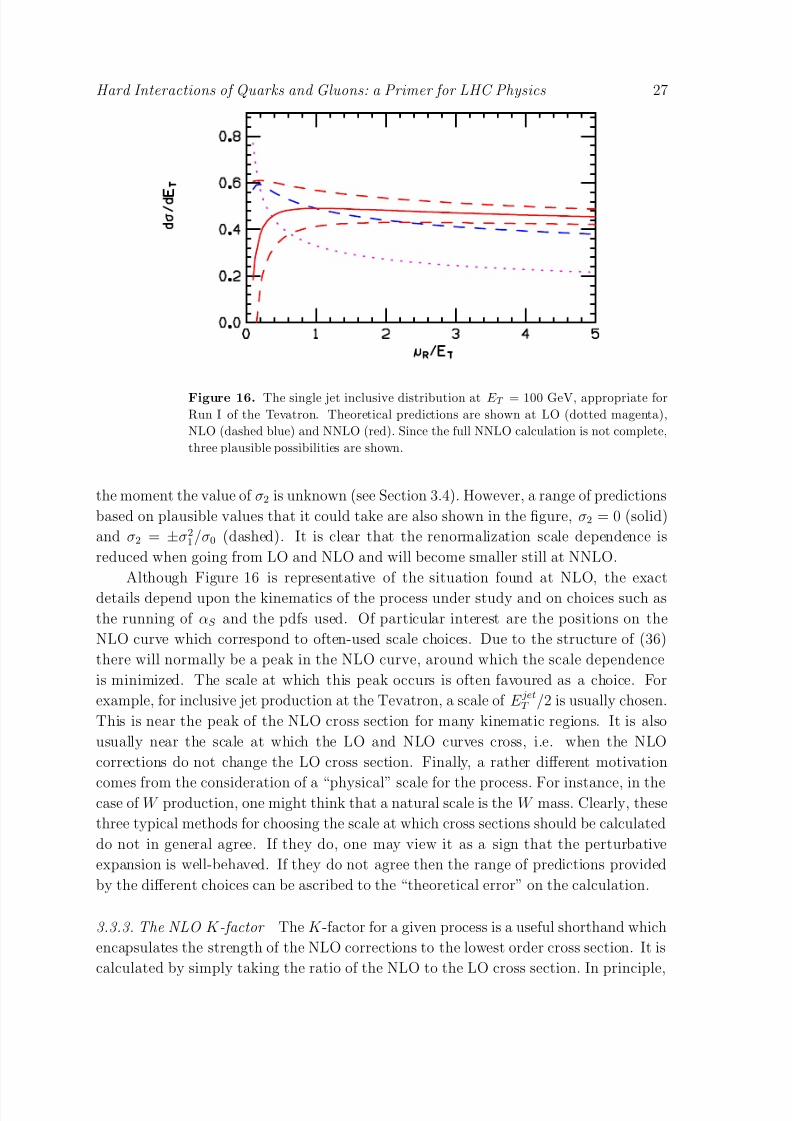
Figure 16. The single jet inclusive distribution at E T = 100 GeV, appropriate forRun I of the Tevatron. Theoretical predictions are shown at LO (dotted magenta),
NLO (dashed blue) and NNLO (red). Since the full NNLO calculation is not complete,
three plausible possibilities are shown.
the moment the value of σ2 is unknown (see Section 3.4). However, a range of predictions
based on plausible values that it could take are also shown in the figure, σ2 = 0 (solid)
and σ2 = ±σ21/σ0 (dashed). It is clear that the renormalization scale dependence is
reduced when going from LO and NLO and will become smaller still at NNLO.
Although Figure 16 is representative of the situation found at NLO, the exact
details depend upon the kinematics of the process under study and on choices such as
the running of αS and the pdfs used. Of particular interest are the positions on the
NLO curve which correspond to often-used scale choices. Due to the structure of (36)
there will normally be a peak in the NLO curve, around which the scale dependence
is minimized. The scale at which this peak occurs is often favoured as a choice. For
example, for inclusive jet production at the Tevatron, a scale of E jetT /2 is usually chosen.
This is near the peak of the NLO cross section for many kinematic regions. It is also
usually near the scale at which the LO and NLO curves cross, i.e. when the NLO
corrections do not change the LO cross section. Finally, a rather different motivation
comes from the consideration of a “physical” scale for the process. For instance, in thecase of W production, one might think that a natural scale is the W mass. Clearly, these
three typical methods for choosing the scale at which cross sections should be calculated
do not in general agree. If they do, one may view it as a sign that the perturbative
expansion is well-behaved. If they do not agree then the range of predictions provided
by the different choices can be ascribed to the “theoretical error” on the calculation.
3.3.3. The NLO K -factor The K -factor for a given process is a useful shorthand which
encapsulates the strength of the NLO corrections to the lowest order cross section. It is
calculated by simply taking the ratio of the NLO to the LO cross section. In principle,
8/3/2019 Hard Interactions of Quarks and Gluons a Primer for LHC Physics
http://slidepdf.com/reader/full/hard-interactions-of-quarks-and-gluons-a-primer-for-lhc-physics 28/118
Hard Interactions of Quarks and Gluons: a Primer for LHC Physics 28
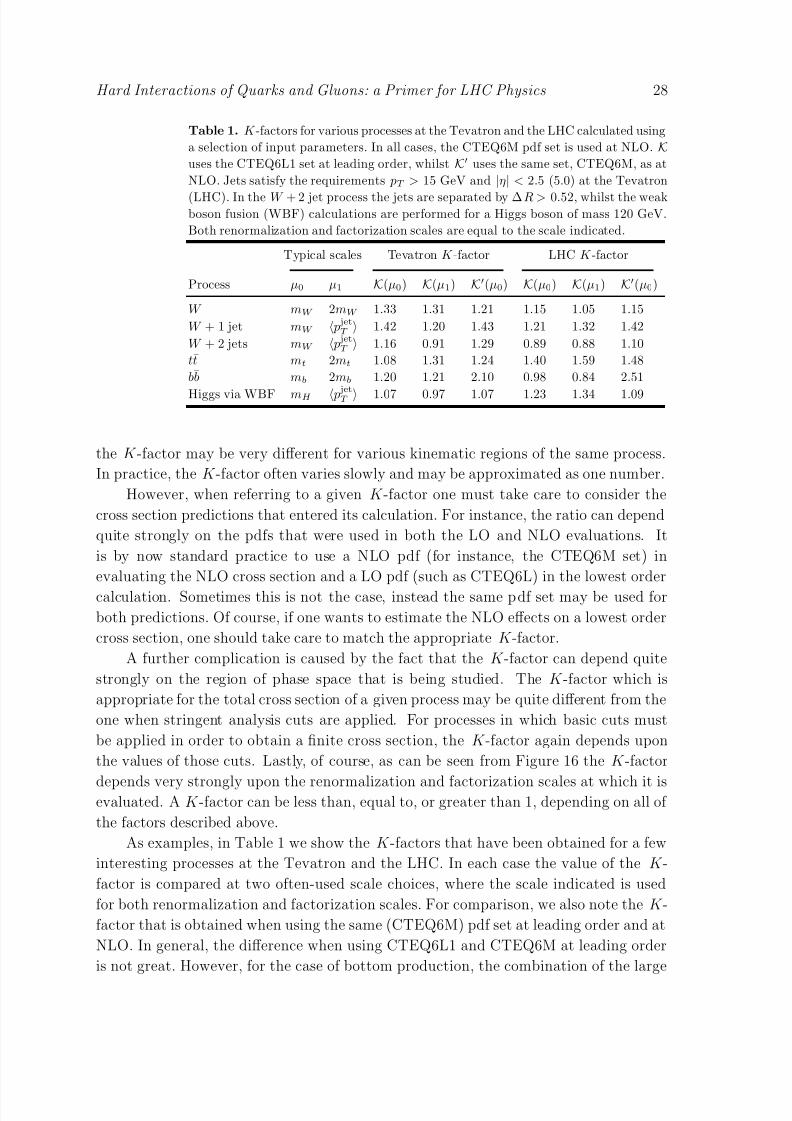
Table 1. K -factors for various processes at the Tevatron and the LHC calculated using
a selection of input parameters. In all cases, the CTEQ6M pdf set is used at NLO. Kuses the CTEQ6L1 set at leading order, whilst K′ uses the same set, CTEQ6M, as at
NLO. Jets satisfy the requirements pT > 15 GeV and
|η
|< 2.5 (5.0) at the Tevatron
(LHC). In the W + 2 jet process the jets are separated by ∆R > 0.52, whilst the weakboson fusion (WBF) calculations are performed for a Higgs boson of mass 120 GeV.
Both renormalization and factorization scales are equal to the scale indicated.
Typical scales Tevatron K -factor LHC K -factor
Process µ0 µ1 K(µ0) K(µ1) K′(µ0) K(µ0) K(µ1) K′(µ0)
W mW 2mW 1.33 1.31 1.21 1.15 1.05 1.15
W + 1 jet mW p jetT 1.42 1.20 1.43 1.21 1.32 1.42
W + 2 jets mW p jetT 1.16 0.91 1.29 0.89 0.88 1.10
tt mt 2mt 1.08 1.31 1.24 1.40 1.59 1.48
bb mb 2mb 1.20 1.21 2.10 0.98 0.84 2.51
Higgs via WBF mH p jetT 1.07 0.97 1.07 1.23 1.34 1.09
the K -factor may be very different for various kinematic regions of the same process.
In practice, the K -factor often varies slowly and may be approximated as one number.
However, when referring to a given K -factor one must take care to consider the
cross section predictions that entered its calculation. For instance, the ratio can depend
quite strongly on the pdfs that were used in both the LO and NLO evaluations. It
is by now standard practice to use a NLO pdf (for instance, the CTEQ6M set) in
evaluating the NLO cross section and a LO pdf (such as CTEQ6L) in the lowest order
calculation. Sometimes this is not the case, instead the same pdf set may be used for
both predictions. Of course, if one wants to estimate the NLO effects on a lowest order
cross section, one should take care to match the appropriate K -factor.
A further complication is caused by the fact that the K -factor can depend quite
strongly on the region of phase space that is being studied. The K -factor which is
appropriate for the total cross section of a given process may be quite different from the
one when stringent analysis cuts are applied. For processes in which basic cuts must
be applied in order to obtain a finite cross section, the K -factor again depends upon
the values of those cuts. Lastly, of course, as can be seen from Figure 16 the K -factor
depends very strongly upon the renormalization and factorization scales at which it isevaluated. A K -factor can be less than, equal to, or greater than 1, depending on all of
the factors described above.
As examples, in Table 1 we show the K -factors that have been obtained for a few
interesting processes at the Tevatron and the LHC. In each case the value of the K -
factor is compared at two often-used scale choices, where the scale indicated is used
for both renormalization and factorization scales. For comparison, we also note the K -
factor that is obtained when using the same (CTEQ6M) pdf set at leading order and at
NLO. In general, the difference when using CTEQ6L1 and CTEQ6M at leading order
is not great. However, for the case of bottom production, the combination of the large
8/3/2019 Hard Interactions of Quarks and Gluons a Primer for LHC Physics
http://slidepdf.com/reader/full/hard-interactions-of-quarks-and-gluons-a-primer-for-lhc-physics 29/118
Hard Interactions of Quarks and Gluons: a Primer for LHC Physics 29
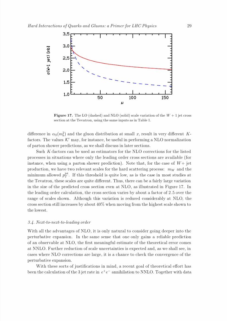
Figure 17. The LO (dashed) and NLO (solid) scale variation of the W + 1 jet cross
section at the Tevatron, using the same inputs as in Table 1.
difference in αS (m2b) and the gluon distribution at small x, result in very different K -
factors. The values K′ may, for instance, be useful in performing a NLO normalization
of parton shower predictions, as we shall discuss in later sections.
Such K -factors can be used as estimators for the NLO corrections for the listed
processes in situations where only the leading order cross sections are available (for
instance, when using a parton shower prediction). Note that, for the case of W + jet
production, we have two relevant scales for the hard scattering process: mW and theminimum allowed p jetT . If this threshold is quite low, as is the case in most studies at
the Tevatron, these scales are quite different. Thus, there can be a fairly large variation
in the size of the predicted cross section even at NLO, as illustrated in Figure 17. In
the leading order calculation, the cross section varies by about a factor of 2.5 over the
range of scales shown. Although this variation is reduced considerably at NLO, the
cross section still increases by about 40% when moving from the highest scale shown to
the lowest.
3.4. Next-to-next-to-leading order
With all the advantages of NLO, it is only natural to consider going deeper into the
perturbative expansion. In the same sense that one only gains a reliable prediction
of an observable at NLO, the first meaningful estimate of the theoretical error comes
at NNLO. Further reduction of scale uncertainties is expected and, as we shall see, in
cases where NLO corrections are large, it is a chance to check the convergence of the
perturbative expansion.
With these sorts of justifications in mind, a recent goal of theoretical effort has
been the calculation of the 3 jet rate in e+e− annihilation to NNLO. Together with data
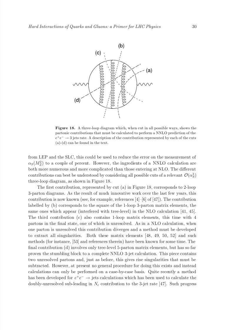
8/3/2019 Hard Interactions of Quarks and Gluons a Primer for LHC Physics
http://slidepdf.com/reader/full/hard-interactions-of-quarks-and-gluons-a-primer-for-lhc-physics 30/118
Hard Interactions of Quarks and Gluons: a Primer for LHC Physics 30
Figure 18. A three-loop diagram which, when cut in all possible ways, shows the
partonic contributions that must be calculated to perform a NNLO prediction of the
e+e− → 3 jets rate. A description of the contribution represented by each of the cuts
(a)-(d) can be found in the text.
from LEP and the SLC, this could be used to reduce the error on the measurement of
αS (M 2Z ) to a couple of percent. However, the ingredients of a NNLO calculation are
both more numerous and more complicated than those entering at NLO. The different
contributions can best be understood by considering all possible cuts of a relevant O(α3S )
three-loop diagram, as shown in Figure 18.
The first contribution, represented by cut (a) in Figure 18, corresponds to 2-loop
3-parton diagrams. As the result of much innovative work over the last few years, this
contribution is now known (see, for example, references [4]–[6] of [47]). The contribution
labelled by (b) corresponds to the square of the 1-loop 3-parton matrix elements, the
same ones which appear (interfered with tree-level) in the NLO calculation [41, 45].
The third contribution (c) also contains 1-loop matrix elements, this time with 4
partons in the final state, one of which is unresolved. As in a NLO calculation, when
one parton is unresolved this contribution diverges and a method must be developedto extract all singularities. Both these matrix elements [48, 49, 50, 52] and such
methods (for instance, [53] and references therein) have been known for some time. The
final contribution (d) involves only tree-level 5-parton matrix elements, but has so far
proven the stumbling block to a complete NNLO 3-jet calculation. This piece contains
two unresolved partons and, just as before, this gives rise singularities that must be
subtracted. However, at present no general procedure for doing this exists and instead
calculations can only be performed on a case-by-case basis. Quite recently a method
has been developed for e+e− → jets calculations which has been used to calculate the
doubly-unresolved sub-leading in N c contribution to the 3-jet rate [47]. Such progress
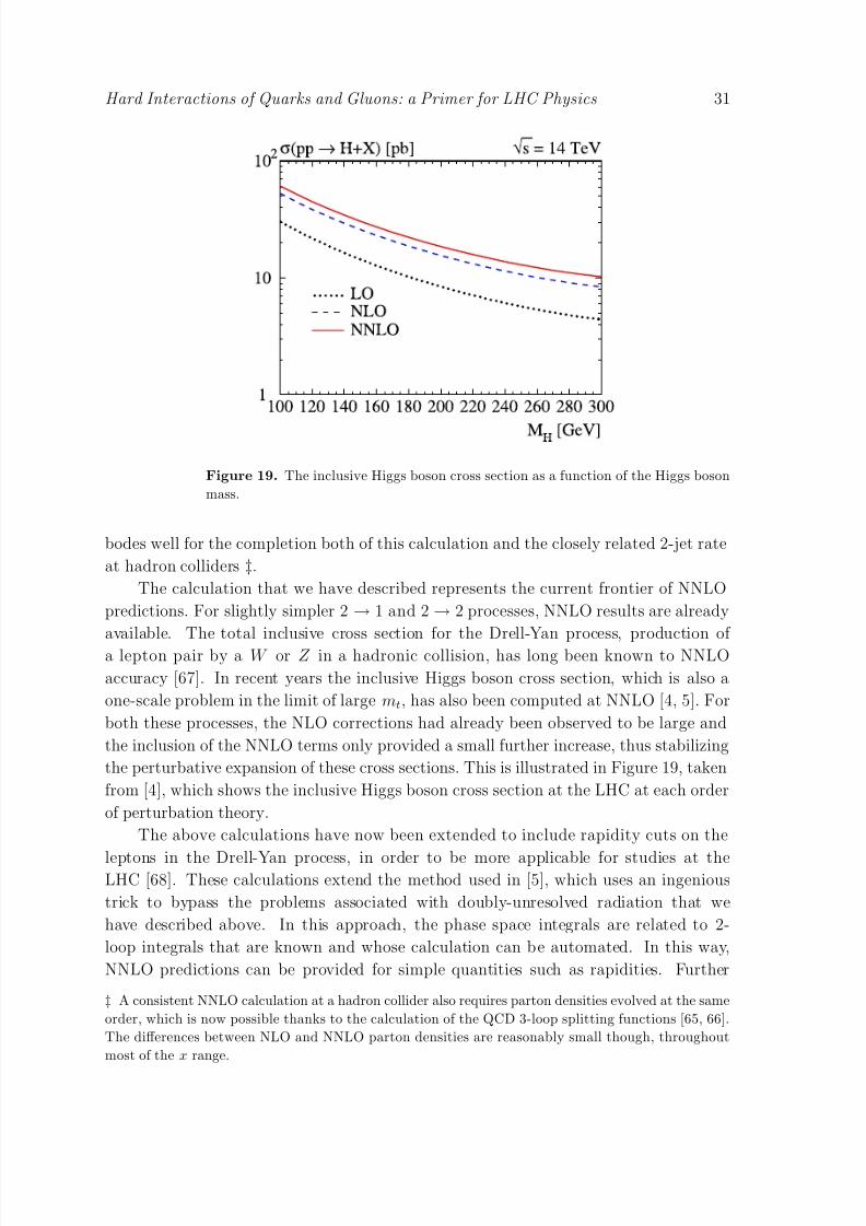
8/3/2019 Hard Interactions of Quarks and Gluons a Primer for LHC Physics
http://slidepdf.com/reader/full/hard-interactions-of-quarks-and-gluons-a-primer-for-lhc-physics 31/118
Hard Interactions of Quarks and Gluons: a Primer for LHC Physics 31
Figure 19. The inclusive Higgs boson cross section as a function of the Higgs boson
mass.
bodes well for the completion both of this calculation and the closely related 2-jet rate
at hadron colliders ‡.
The calculation that we have described represents the current frontier of NNLO
predictions. For slightly simpler 2 → 1 and 2 → 2 processes, NNLO results are already
available. The total inclusive cross section for the Drell-Yan process, production of
a lepton pair by a W or Z in a hadronic collision, has long been known to NNLO
accuracy [67]. In recent years the inclusive Higgs boson cross section, which is also a
one-scale problem in the limit of large mt, has also been computed at NNLO [4, 5]. For
both these processes, the NLO corrections had already been observed to be large and
the inclusion of the NNLO terms only provided a small further increase, thus stabilizing
the perturbative expansion of these cross sections. This is illustrated in Figure 19, taken
from [4], which shows the inclusive Higgs boson cross section at the LHC at each order
of perturbation theory.
The above calculations have now been extended to include rapidity cuts on the
leptons in the Drell-Yan process, in order to be more applicable for studies at theLHC [68]. These calculations extend the method used in [5], which uses an ingenious
trick to bypass the problems associated with doubly-unresolved radiation that we
have described above. In this approach, the phase space integrals are related to 2-
loop integrals that are known and whose calculation can be automated. In this way,
NNLO predictions can be provided for simple quantities such as rapidities. Further
‡ A consistent NNLO calculation at a hadron collider also requires parton densities evolved at the same
order, which is now possible thanks to the calculation of the QCD 3-loop splitting functions [65, 66].
The differences between NLO and NNLO parton densities are reasonably small though, throughout
most of the x range.

8/3/2019 Hard Interactions of Quarks and Gluons a Primer for LHC Physics
http://slidepdf.com/reader/full/hard-interactions-of-quarks-and-gluons-a-primer-for-lhc-physics 32/118
Hard Interactions of Quarks and Gluons: a Primer for LHC Physics 32
developments now allow for the introduction of generic cuts, paving the way for more
detailed experimental analyses [69].
3.5. All orders approaches
Rather than systematically calculating to higher and higher orders in the perturbative
expansion of a given observable, a number of different “all-orders” approaches are also
commonly used to describe the phenomena observed at high-energy colliders. These
alternative descriptions are typically most useful under a different set of conditions than
a fixed order approach. The merging of such a description with fixed-order calculations,
in order to offer the best of both worlds, is of course highly desirable.
Resummation is one such approach, in which the dominant contributions from each
order in perturbation theory are singled out and “resummed” by the use of an evolution
equation. Near the boundaries of phase space, fixed order predictions break down due
to large logarithmic corrections, as we have seen above. A straightforward example is
provided by the production of a vector boson at hadron colliders. In this case, two
large logarithms can be generated. One is associated with the production of the vector
boson close to threshold (s = Q2) and takes the form αnS log2n−1(1 − z)/(1 − z), where
z = Q2/s − 1. The other logarithm, as illustrated earlier, is associated with the recoil
of the vector boson at very small transverse momenta pT , so that logarithms appear as
αnS log2n−1(Q2/p2T ), c.f. (22). Various methods for performing these resummations are
available [70, 71, 72, 73, 74, 75, 76, 77], with some techniques including both effects at
the same time [78, 79, 80]. As we shall see later, the inclusion of such effects is crucial in
order to describe data at the Tevatron and to estimate genuine non-perturbative effects.The ResBos program § [81] is a publicly available program that provides NLO resummed
predictions for processes such as W,Z,γγ and Higgs boson production at hadron-hadron
colliders. Resummation is of course not restricted to the study of these processes alone,
with much progress recently in the resummation of event shape variables at hadron
colliders (for a recent review, see [82]).
The expression for the W boson transverse momentum in which the leading
logarithms have been resummed to all orders is given by (c.f. (22) and (30)),
dσ
dp2T = σ
d
dp2T exp−αS C F
2πlog2 M 2W /p2T . (40)
This describes the basic shape for the transverse distribution for W production, which
is shown in Figure 20. Note that in this approximation the p2T distribution vanishes as
pT → 0, a feature which is not seen experimentally. However this can be explained by
the fact that the only configuration included as pT → 0 is the one in which all emitted
gluons are soft. In reality (and in a more complete resummed prediction), multiple
gluon emissions with a vector sum equal to pT contribute and fill in the dip at pT = 0.
A different, but related, approach is provided by parton showers. The numerical
implementation of a parton shower, for instance in the programs PYTHIA, HERWIG
§http://hep.pa.msu.edu/people/cao/ResBos-A.html
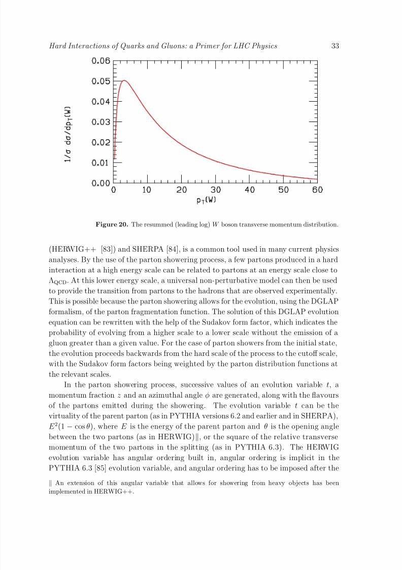
8/3/2019 Hard Interactions of Quarks and Gluons a Primer for LHC Physics
http://slidepdf.com/reader/full/hard-interactions-of-quarks-and-gluons-a-primer-for-lhc-physics 33/118
Hard Interactions of Quarks and Gluons: a Primer for LHC Physics 33
Figure 20. The resummed (leading log) W boson transverse momentum distribution.
(HERWIG++ [83]) and SHERPA [84], is a common tool used in many current physics
analyses. By the use of the parton showering process, a few partons produced in a hard
interaction at a high energy scale can be related to partons at an energy scale close to
ΛQCD. At this lower energy scale, a universal non-perturbative model can then be used
to provide the transition from partons to the hadrons that are observed experimentally.
This is possible because the parton showering allows for the evolution, using the DGLAPformalism, of the parton fragmentation function. The solution of this DGLAP evolution
equation can be rewritten with the help of the Sudakov form factor, which indicates the
probability of evolving from a higher scale to a lower scale without the emission of a
gluon greater than a given value. For the case of parton showers from the initial state,
the evolution proceeds backwards from the hard scale of the process to the cutoff scale,
with the Sudakov form factors being weighted by the parton distribution functions at
the relevant scales.
In the parton showering process, successive values of an evolution variable t, a
momentum fraction z and an azimuthal angle φ are generated, along with the flavours
of the partons emitted during the showering. The evolution variable t can be the
virtuality of the parent parton (as in PYTHIA versions 6.2 and earlier and in SHERPA),
E 2(1 − cos θ), where E is the energy of the parent parton and θ is the opening angle
between the two partons (as in HERWIG), or the square of the relative transverse
momentum of the two partons in the splitting (as in PYTHIA 6.3). The HERWIG
evolution variable has angular ordering built in, angular ordering is implicit in the
PYTHIA 6.3 [85] evolution variable, and angular ordering has to be imposed after the
An extension of this angular variable that allows for showering from heavy objects has been
implemented in HERWIG++.

8/3/2019 Hard Interactions of Quarks and Gluons a Primer for LHC Physics
http://slidepdf.com/reader/full/hard-interactions-of-quarks-and-gluons-a-primer-for-lhc-physics 34/118
Hard Interactions of Quarks and Gluons: a Primer for LHC Physics 34
fact for the PYTHIA 6.2 evolution variable. Angular ordering represents an attempt to
simulate more precisely those higher order contributions that are enhanced due to soft
gluon emission (colour coherence). Fixed order calculations explicitly account for colour
coherence, while parton shower Monte Carlos that include colour flow information model
it only approximately.
Note that with parton showering, we in principle introduce two new scales, one for
initial state parton showering and one for the shower in the final state. In the PYTHIA
Monte Carlo, the scale used is most often related to the maximum virtuality in the
hard scattering, although a larger ad hoc scale, such as the total centre-of-mass energy,
can also be chosen by the user. The HERWIG showering scale is determined by the
specific colour flow in the hard process and is related to the invariant mass of the colour
connected partons.
We can write an expression for the Sudakov form factor of an initial state parton
in the form shown in (41), where t is the hard scale, t0 is the cutoff scale and P (z) isthe splitting function for the branching under consideration.
∆(t) ≡ exp
− tt0
dt′
t′
dz
z
αS
2πP (z)
f (x/z,t)
f (x, t)
(41)
The Sudakov form factor has a similar form for the final state but without the pdf
weighting. The introduction of the Sudakov form factor resums all the effects of soft and
collinear gluon emission, which leads to well-defined predictions even in these regions.
However, this ability comes at a price. Although the soft and collinear regions are
logarithmically enhanced and thus the dominant effect, this method does not attempt
to correctly include the non-singular contributions that are due to large energy, wideangle gluon emission. We shall return to this discussion later.
3.5.1. Sudakov form factors As discussed in the previous section, the Sudakov form
factor gives the probability for a parton to evolve from a harder scale to a softer scale
without emitting a parton harder than some resolution scale, either in the initial state
or in the final state. Sudakov form factors form the basis for both parton showering and
resummation. Typically, the details of the form factors are buried inside the interior of
such programs. It is useful, however, to generate plots of the initial state Sudakov form
factors for the kinematic conditions encountered at both the Tevatron and LHC. Such
plots indicate the likelihood for the non-radiation of gluons from the initial state partons,and thus conversely for the radiation of at least one such gluon. Thus, they can also serve
as a handy reference for the probability of jets from initial state radiation. A Sudakov
form factor will depend on: (1) the parton type (quark or gluon), (2) the momentum
fraction x of the initial state parton, (3) the hard and cutoff scales for the process and
(4) the resolution scale for the emission. Several examples are discussed below. These
plots were generated with the HERWIG++ parton shower formalism [86] ¶.
¶ We thank Stefan Gieseke for providing us with the relevant information.

8/3/2019 Hard Interactions of Quarks and Gluons a Primer for LHC Physics
http://slidepdf.com/reader/full/hard-interactions-of-quarks-and-gluons-a-primer-for-lhc-physics 35/118
Hard Interactions of Quarks and Gluons: a Primer for LHC Physics 35
(GeV/c)gluon
TP
10 15 20 25 30
S u d a k o v f o r m f a
c t o r
0
0.2
0.4
0.6
0.8
1
ScaleT
Jet20 corrected Mulitple Interactions and Hadron P
(GeV/c)gluon
TP
10 15 20 25 30
S u d a k o v f o r m f a
c t o r
0
0.2
0.4
0.6
0.8
1
10 15 20 25 300
0.2
0.4
0.6
0.8
1
Figure 21. The Sudakov form factors for initial state gluons at a hard scale of 100 GeV
as a function of the transverse momentum of the emitted gluon. The form factors arefor (top to bottom) parton x values of 0.3, 0.1, 0.03, 0.01, 0.001 and 0.0001.
(GeV/c)gluon
TP
10 15 20 25 30
S u d a k o v f o r m f a
c t o r
0
0.2
0.4
0.6
0.8
1
ScaleT
Jet20 corrected Mulitple Interactions and Hadron P
(GeV/c)gluon
TP
10 15 20 25 30
S u d a k o v f o r m f a
c t o r
0
0.2
0.4
0.6
0.8
1
Figure 22. The Sudakov form factors for initial state gluons at a hard scale of 500 GeV
as a function of the transverse momentum of the emitted gluon. The form factors are
for (top to bottom) parton x values of 0.3, 0.1, 0.03, 0.01, 0.001 and 0.0001.
In Figure 21 are plotted the Sudakov form factors for the splitting g → gg, ata hard scale of 100 GeV, and for several different values of the parton x value. The
form factors are plotted versus the resolution scale for the emitted gluon, which can be
thought of roughly as the transverse momentum of the emitted gluon. The probability
for no emission decreases as the transverse momentum of the emitted gluon decreases
and as the parton x decreases. The former is fairly obvious; the latter may not be so.
The smaller the value of the initial parton momentum fraction, the larger is the possible
phase space for gluon emission.
For example, the probability for a gluon with an x value of 0.03 to evolve from
100 GeV down to 10 GeV without emitting a gluon of 10 GeV or greater can be read

8/3/2019 Hard Interactions of Quarks and Gluons a Primer for LHC Physics
http://slidepdf.com/reader/full/hard-interactions-of-quarks-and-gluons-a-primer-for-lhc-physics 36/118
Hard Interactions of Quarks and Gluons: a Primer for LHC Physics 36
(GeV/c)gluon
TP
10 15 20 25 30
S u d a k o v f o r m f a
c t o r
0
0.2
0.4
0.6
0.8
1
ScaleT
Jet20 corrected Mulitple Interactions and Hadron P
(GeV/c)gluon
TP
10 15 20 25 30
S u d a k o v f o r m f a
c t o r
0
0.2
0.4
0.6
0.8
1
Figure 23. The Sudakov form factors for initial state quarks at a hard scale of
100 GeV as a function of the transverse momentum of the emitted gluon. The formfactors are for (top to bottom) parton x values of 0.3, 0.1 and 0.03.
off the plot as being 60%; thus the probability for at least one such emission is 40%.
This is another example where the probability of emission of a hard gluon is enhanced
by a logarithm (in this case the ratio of the hard scale to the resolution scale) compared
to the naive expectation of a factor of αS . The probability of emission of such a gluon
from an initial state gluon on the opposite side of the collision would of course be the
same.
In Figure 22, the same Sudakov form factors are plotted but now using a hard scaleof 500 GeV. The increased probability of a hard gluon emission can be observed. In
Figures 23 and 24, the Sudakov form factors are plotted for the hard scales of 100 GeV
and 500 GeV as before, but now for the splitting q → qg. The probability of no emission
is larger, due to the smaller colour factor of the initial state quark compared to the gluon.
Note that the form factor curves for x values of less than 0.03 have not been plotted
as they would essentially lie on top of the x = 0.03 curve. It is not the smaller colour
factor that causes the difference with the gluon but rather the splitting function. The
splitting function for g → gg has singularities both as z → 0 and as z → 1, while the
q
→qg has only the z
→1 singularity. Thus, for the q
→qg splitting, there is not much
to gain from decreasing x on a logarithmic scale, as there is no singularity at z = 0 inthe splitting function.
3.6. Partons and jet algorithms
In the detectors of experiments at the Tevatron and the LHC, collimated beams of
particles are observed. In order to categorize these events, the hadrons are collected
into jets using a jet algorithm. To make a comparison with a theoretical calculation of
the types we have been discussing, it is necessary to also apply a jet algorithm at the
parton level. Ideally, one would like an algorithm which yields similar results at the

8/3/2019 Hard Interactions of Quarks and Gluons a Primer for LHC Physics
http://slidepdf.com/reader/full/hard-interactions-of-quarks-and-gluons-a-primer-for-lhc-physics 37/118
Hard Interactions of Quarks and Gluons: a Primer for LHC Physics 37
(GeV/c)gluon
TP
10 15 20 25 30
S u d a k o v f o r m f a
c t o r
0
0.2
0.4
0.6
0.8
1
ScaleT
Jet20 corrected Mulitple Interactions and Hadron P
(GeV/c)gluon
TP
10 15 20 25 30
S u d a k o v f o r m f a
c t o r
0
0.2
0.4
0.6
0.8
1
Figure 24. The Sudakov form factors for initial state quarks at a hard scale of
500 GeV as a function of the transverse momentum of the emitted gluon. The formfactors are for (top to bottom) parton x values of 0.3, 0.1 and 0.03.
experimental (hadron) and theoretical (parton) levels. The goal is to characterize the
short-distance physics event-by-event, in terms of the jets formed by the algorithm.
There are two essential stages for any jet algorithm. First, the objects belonging to
a cluster are identified. Second, the kinematic variables defining the jet are calculated
from the objects defining the cluster. The two stages are independent. For the latter
stage, using the jet algorithms developed for Run 2 at the Tevatron, the jet kinematic
properties are defined (using a 4-vector recombination scheme) in terms of: p jet, p
jet
T ,y jet and φ jet.
At the experimental or simulated data level, jet algorithms cluster together objects
such as particles or energies measured in calorimeter cells. At the theoretical level,
partons are clustered. The goal of a jet algorithm is to produce similar results no
matter the level it is applied. For a 2 → 2 LO calculation, a jet consists simply of 1
parton and no jet algorithm is necessary. As more partons are added to a calculation, the
complexity of a jet grows and approaches the complexity found either in parton shower
Monte Carlos or in data. For all situations in which a jet can consist of more than 1
parton, a completely specified jet algorithm is needed. The clustering algorithms rely on
the association of these objects based on transverse momentum (the kT algorithm) [87]or angles (the cone algorithm), relative to a jet axis.
For NLO calculations, as for example W + 2 jets, a jet can consist of either 1 or
2 partons. Cone jet algorithms as currently used by the Tevatron experiments require
the use of seeds (initial directions for jet cones)as the starting points for jet searches.
For a partonic level final state, the seeds are the partons themselves. The Run 2 cone
algorithm (midpoint) places additional seeds between stable cones having a separation of
less than twice the size of the clustering cones; the use of these additional seeds removes
problems with infrared instabilities in theoretical calculations. Without a midpoint seed,
8/3/2019 Hard Interactions of Quarks and Gluons a Primer for LHC Physics
http://slidepdf.com/reader/full/hard-interactions-of-quarks-and-gluons-a-primer-for-lhc-physics 38/118
Hard Interactions of Quarks and Gluons: a Primer for LHC Physics 38
a jet could be formed/not formed depending on the presence of a soft gluon between two
hard partons; this leads to an undesirable logarithmic dependence of the cross section
on the energy of this soft gluon.
With a cone algorithm, two partons are nominally included in the same jet if they
are within Rcone of the pT -weighted jet centroid, and so within a maximum ∆R of 1.4
of each other if a cone radius of 0.7 is used. However, it was noted that with the
experimental jet algorithms used at the Tevatron, that two jets would not be merged
into a single jet if they were separated by a distance greater than 1 .3 times the cone
radius. Thus, a phenomenological parameter Rsep = 1.3 was added to the theoretical
prediction; two partons would not be merged into a single jet if they were separated
by more than Rsep × Rcone from each other. So, in a parton level calculation having
at most 3 partons in the final state, two partons are merged into the same jet if they
are within Rcone of the pT -weighted jet centroid and within Rsep × Rcone of each other;
otherwise the two partons are termed separate jets. Thus, for W + 2 jet production atNLO, the final state can consist of either 2 or 3 partons. The 2 parton final state will
always be reconstructed as 2 jets; the 3 parton final state may be reconstructed as either
2 or 3 jets depending on whether the 2 lowest pT partons satisfy the clustering criteria
described above. Note that for some partonic level programs such as JETRAD [88] ,
the clustering is not performed prior to the evaluation of the matrix element. Thus,
the individual transverse momenta of the jets are also not known at this time; only the
transverse momentum of the highest pT parton, which by momentum conservation must
remain unclustered, is known. For this reason, a renormalization/factorization scale of
pmaxT (the pT of this parton) is used in calculating the cross section for each jet.
A schematic diagram indicating the regions in which two partons will be includedin the same jet is shown in Figure 25 [89]. All partons within Rcone of each other
will always be clustered in the same jet. This corresponds to the region labeled I. An
ideal cone algorithm acting on data would cluster together only the underlying parton
level configurations corresponding to region II and not configurations in region III.
However, as will be seen in Section 5, the stochastic character of the parton showering
and hadronization process makes such a clean division difficult in either real data or
with a parton shower Monte Carlo. Because the matrix element for the emission of an
additional real parton has both a collinear and soft pole, configurations in regions II and
III with two partons having ∆R near 0.7 and z near 0 will be most heavily populated.The fractional contribution to the inclusive jet cross section of the merged two parton
configurations in Region II is proportional to αS ( p2T ) and thus should decrease with
increasing jet transverse momentum.
The kT algorithm [87] is conceptually simpler at all levels. Two partons (or particles,
or energies) in calorimeter towers are combined if their relative transverse momentum is
less than a given measure. At the parton level, each parton is considered as a proto-jet.
The quantities k2T,i = P 2T,i and kT,(i,j) = min(P 2T,i, P 2T,j).∆R2
i,j/D2 are computed for each
parton and each pair of partons respectively. P T,i is the transverse momentum of the
ith parton, ∆Ri,j is the distance (in y, φ space) between each pair of partons, and D is

8/3/2019 Hard Interactions of Quarks and Gluons a Primer for LHC Physics
http://slidepdf.com/reader/full/hard-interactions-of-quarks-and-gluons-a-primer-for-lhc-physics 39/118
Hard Interactions of Quarks and Gluons: a Primer for LHC Physics 39
Figure 25. The parameter space (d, Z ) for which two partons will be merged into a
single jet.
a parameter that controls the size of the jet. If the smallest of the above quantities is
a kT,i then that parton becomes a jet; if the smallest quantity is a kT,(i,j), then the two
partons are combined into a single proto-jet by summing their four-vector components.
In a NLO inclusive jet calculation, the two lowest pT partons may be combined into a
single jet, and thus the final state can consist of either 2 or 3 jets, as was also true for
the case of the cone algorithm. The kT algorithm merges two partons into a single jet if
∆Rij ¡ D. In Figure 25, if D is set to Rcone, the kT algorithm would merge partons for
which d ¡ R, or in the language used above for the cone algorithm, Rsep = 1. Since the
cone algorithm merges the partons not only for d ¡ R, but also in the triangular regionabove the line d = R(1 + z), a cone jet cross section at the parton level, for cone radius
R, will necessarily be larger than a kT jet cross section with D=R. If we use an Rsep
value of 1.3 rather than 2 for the cone algorithm, the difference in relative cross sections
between the two algorithms will be reduced. As we will see in Section 5, this relative
behaviour of the two algorithms does not hold at the hadron level.
The assumption we are making above is that the jets of hadrons measured in
a collider experiment can be represented by the 1 or 2 partons that comprise a jet
at the NLO theoretical level. That is, the 1 or 2 partons present in a NLO jet
effectively represent the many partons produced by a parton shower. For example,
an equivalent description of the jet shape is provided by the two types of calculation.This approximation has been borne out in practice with one remaining correction being
necessary. Partons whose trajectories lie inside the jet cone eventually produce hadrons,
some of which may land outside the cone due to the fragmentation process. The
fragmentation correction takes a particularly simple form. For a cone of radius 0.7,
each jet loses approximately 1 GeV due to fragmentation, basically independent of the
jet transverse energy. The naıve assumption might be that the energy outside the cone
due to fragmentation would rise with the jet energy; however, the jet becomes narrower
at higher E T , leading to a roughly constant amount of energy in the outermost portions

8/3/2019 Hard Interactions of Quarks and Gluons a Primer for LHC Physics
http://slidepdf.com/reader/full/hard-interactions-of-quarks-and-gluons-a-primer-for-lhc-physics 40/118
Hard Interactions of Quarks and Gluons: a Primer for LHC Physics 40
of the jet. As will be described in Section 5, corrections also need to be applied to the
data or to the theory to take into account the underlying event energy.
A quantity related to the jet shape is the jet mass. To first order, the jet mass, like
the jet shape, is determined by the hardest gluon emission. This emission is governed
by the Sudakov form factor, and thus the jet mass distribution should fall roughly as
1/m2, with modification at the two endpoints. There will be a Sudakov suppression for
low jet masses (corresponding to little or no gluon emission), and at high jet masses the
jet algorithm will tend to break the jet up into two separate jets. The average mass for
this falling distribution will be approximately 10–15% of the transverse momentum of
the jet.
3.7. Merging parton showers and fixed order
As we have discussed previously in Section 3.5, parton showers provide an excellent
description in regions which are dominated by soft and collinear gluon emission. On the
other hand, matrix element calculations provide a good description of processes where
the partons are energetic and widely separated and, in addition, include the effects of
interference between amplitudes with the same external partons. But, on the other
hand, the matrix element calculations do not take into account the interference effects
in soft and collinear gluon emissions which cannot be resolved, and which lead to a
Sudakov suppression of such emissions.
Clearly, a description of a hard interaction which combines the two types of
calculations would be preferable. For this combination to take place, there first needs
to be a universal formalism that allows the matrix element calculation to “talk” to theparton shower Monte Carlo. Such a universal formalism was crafted during the Les
Houches Workshop on Collider Physics in 2001 and the resulting “Les Houches Accord”
is in common use [90]. The accord specifies an interface between the matrix element
and the parton shower program which provides information on the parton 4-vectors, the
mother-daughter relationships, and the spin/helicities and colour flow. It also points to
intermediate particles whose mass should be preserved in the parton showering. All of
the details are invisible to the casual user and are intended for the matrix element/parton
shower authors.
Some care must be taken however, as a straight addition of the two techniques
would lead to double-counting in kinematic regions where the two calculations overlap.There have been many examples where matrix element information has been used to
correct the first or the hardest emission in a parton shower. There are also more general
techniques that allow matrix element calculations and parton showers to each be used
in kinematic regions where they provide the best description of the event properties and
that avoid double-counting. One such technique is termed CKKW [91].
With the CKKW technique, the matrix element description is used to describe
parton branchings at large angle and/or energy, while the parton shower description is
used for the smaller angle, lower energy emissions. The phase space for parton emission is

8/3/2019 Hard Interactions of Quarks and Gluons a Primer for LHC Physics
http://slidepdf.com/reader/full/hard-interactions-of-quarks-and-gluons-a-primer-for-lhc-physics 41/118
Hard Interactions of Quarks and Gluons: a Primer for LHC Physics 41
thus divided into two regions, matrix element dominated and parton shower dominated,
using a resolution parameter dini. The argument of αS at all of the vertices is chosen
to be equal to the resolution parameter di at which the branching has taken place and
Sudakov form factors are inserted on all of the quark and gluon lines to represent the
lack of any emissions with a scale larger than dini between vertices. The di represent
a virtuality or energy scale. Parton showering is used to produce additional emissions
at scales less than dini. For a typical matching scale, approximately 10% of the n-jet
cross section is produced by parton showering from the n-1 parton matrix element; the
rest arises mostly from the n-parton matrix element. A schematic representation of the
CKKW scheme is shown in Figure 26 for the case of W + jets production at a hadron-
hadron collider. A description of a W + 2 jet event in the NLO formalism is also shown
for comparison.
The CKKW procedure provides a matching between the matrix element and parton
shower that should be correct to the next-to-leading-logarithm (NLL) level. There are,however, a number of choices that must be made in the matching procedure that do
not formally affect the logarithmic behaviour but do affect the numerical predictions,
on the order of 20–30%. The CKKW procedure gives the right amount of radiation but
tends to put some of it in the wrong place with the wrong colour flow. Variations that
result from these choices must be considered as part of the systematic error inherent in
the CKKW process. This will be discussed further in Section 5.
For the CKKW formalism to work, matrix element information must in principle
be available for any number n of partons in the final state. Practically speaking, having
information available for n up to 4 is sufficient for the description of most events at the
Tevatron or LHC. The CKKW formalism is implemented in the parton shower MonteCarlo SHERPA [92] and has also been used for event generation at the Tevatron and
LHC using the Mrenna-Richardson formalism [94]. An approximate version of CKKW
matching (the “MLM approach” +) is available in ALPGEN 2.0 [18].
3.8. Merging NLO calculations and parton showers
A combination of NLO calculations with parton shower Monte Carlos leads to the
best of both worlds. The NLO aspect leads to a correct prediction for the rate of the
process and also improves the description of the first hard parton emission. The parton
shower aspect provides a sensible description of multiple/soft collinear emissions witha final state consisting of hadrons, which can then be input to a detector simulation.
In a parton shower interface, a specific subtraction scheme must be implemented to
preserve the NLO cross section. As each parton shower Monte Carlo may produce
a different real radiation component, the subtraction scheme must necessarily depend
on the Monte Carlo program to which the matrix element program is matched. The
presence of interference effects with NLO calculations requires that a relatively small
fraction (∼ 10%) of events have negative weights (of value −1).
+ ...which one of the authors takes credit for naming.

8/3/2019 Hard Interactions of Quarks and Gluons a Primer for LHC Physics
http://slidepdf.com/reader/full/hard-interactions-of-quarks-and-gluons-a-primer-for-lhc-physics 42/118
Hard Interactions of Quarks and Gluons: a Primer for LHC Physics 42
αs(d5)
αs(d4)
αs(d3)
αs(mW )
αs(mW )
αs(d2)
αs(d6)
αs(d1)
Figure 26. In the NLO formalism, the same scale, proportional to the hardness of
the process, is used for each QCD vertex. For the case of the W + 2 jet diagram
shown above to the left, a scale related to the mass of the W boson, or to the average
transverse momentum of the produced jets, is typically used. The figure to the right
shows the results of a simulation using the CKKW formalism. Branchings occur at the
vertices with resolution parameters di, where d1 > d2 >> dini > d3 > d4 > d5 > d6Branchings at the vertices 1-2 are produced with matrix element information while the
branchings at vertices 3-6 are produced by the parton shower.
Several groups have worked on the subject to consistently combine partonic NLO
calculations with parton showers.
• Collins, Zu [95, 96]
• Frixione, Nason, Webber (MC@NLO) [97, 98, 99]
• Kurihara, Fujimoto, Ishikawa, Kato, Kawabata, Munehisa, Tanaka [100]
•Kramer, Soper [101, 102, 103]
• Nagy, Soper [104, 105]
MC@NLO is the only publicly available program that combines NLO calculations
with parton showering and hadronization. The HERWIG Monte Carlo is used for the
latter. The use of a different Monte Carlo, such as PYTHIA, would require a different
subtraction scheme for the NLO matrix elements. The processes included to date are:
(W,Z,γ ∗,H,bb,tt,HW,HZ,WW,WZ,ZZ ). Recently, single top hadroproduction has
been added to MC@NLO [106]. This is the first implementation of a process that
has both initial- and final-state singularities. This allows a more general category of
additional processes to be added in the future. Work is proceeding on the addition of

8/3/2019 Hard Interactions of Quarks and Gluons a Primer for LHC Physics
http://slidepdf.com/reader/full/hard-interactions-of-quarks-and-gluons-a-primer-for-lhc-physics 43/118
Hard Interactions of Quarks and Gluons: a Primer for LHC Physics 43
inclusive jet production and the production of a Higgs boson via W W fusion. Adding
spin correlations to a process increases the level of difficulty but is important for
processes such as single top production.
If, in addition, the CKKW formalism could be used for the description of hard
parton emissions, the utility and accuracy of a NLO Monte Carlo could be greatly
increased. The merger of these two techniques should be possible in Monte Carlos
available by the time of the LHC turn-on.
4. Parton distribution functions
4.1. Introduction
As mentioned in Section 2, the calculation of the production cross sections at hadron
colliders for both interesting physics processes and their backgrounds relies upon a
knowledge of the distribution of the momentum fraction x of the partons (quarks andgluons) in a proton in the relevant kinematic range. These parton distribution functions
(pdfs) can not be calculated perturbatively but rather are determined by global fits to
data from deep inelastic scattering (DIS), Drell-Yan (DY), and jet production at current
energy ranges. Two major groups, CTEQ [11] and MRST [10], provide semi-regular
updates to the parton distributions when new data and/or theoretical developments
become available. In addition, there are also pdfs available from Alekhin [107] and from
the two HERA experiments [108, 109, 110, 111]. The newest pdfs, in most cases, provide
the most accurate description of the world’s data, and should be utilized in preference
to older pdf sets.
4.2. Processes involved in global analysis fits
Measurements of deep-inelastic scattering (DIS) structure functions (F 2, F 3) in lepton-
hadron scattering and of lepton pair production cross sections in hadron-hadron
collisions provide the main source of information on quark distributions f q/p(x, Q2)
inside hadrons. At leading order, the gluon distribution function f g/p(x, Q2) enters
directly in hadron-hadron scattering processes with jet final states. Modern global
parton distribution fits are carried out to NLO and in some cases to NNLO, which
allows αS (Q
2
), f q/p(x, Q
2
) and f g/p(x, Q
2
) to all mix and contribute in the theoreticalformulae for all processes. Nevertheless, the broad picture described above still holds to
some degree in global pdf analyses.
The data from DIS, DY and jet processes utilized in pdf fits cover a wide range
in x and Q2. HERA data (H1 [54]+ZEUS [55]) are predominantly at low x, while the
fixed target DIS [57, 58, 59, 60, 61] and DY [62, 56] data are at higher x. Collider
jet data [63, 64] cover a broad range in x and Q2 by themselves and are particularly
important in the determination of the high x gluon distribution. There is considerable
overlap, however, among the datasets with the degree of overlap increasing with time
as the statistics of the HERA experiments increase. Parton distributions determined at

8/3/2019 Hard Interactions of Quarks and Gluons a Primer for LHC Physics
http://slidepdf.com/reader/full/hard-interactions-of-quarks-and-gluons-a-primer-for-lhc-physics 44/118
Hard Interactions of Quarks and Gluons: a Primer for LHC Physics 44
a given x and Q2 ‘feed-down’ or evolve to lower x values at higher Q2 values. DGLAP-
based NLO (and NNLO) pQCD should provide an accurate description of the data (and
of the evolution of the parton distributions) over the entire kinematic range present in
current global fits. At very low x and Q, DGLAP evolution is believed to be no longer
applicable and a BFKL [174, 175, 176, 177] description must be used. No clear evidence
of BFKL physics is seen in the current range of data; thus all global analyses use
conventional DGLAP evolution of pdfs.
Many processes have been calculated to NLO and there is the possibility of including
data from these processes in global fits. For example, the rapidity distributions for W +,
W − and Z production at the Tevatron and LHC should prove to be very useful in
constraining u and d valence and sea quarks.
There is a remarkable consistency between the data in the pdf fits and the
perturbative QCD theory fit to them. Both the CTEQ and MRST groups use over
2000 data points in their global pdf analyses and the χ2
/DOF for the fit of theory todata is on the order of unity. For most of the data points, the statistical errors are
smaller than the systematic errors, so a proper treatment of the systematic errors and
their bin-to-bin correlations is important.
The accuracy of the extrapolation to higher Q2 depends on the accuracy of the
original measurement, any uncertainty on αS (Q2) and the accuracy of the evolution
code. Most global pdf analyses are carried out at NLO; recently, the DGLAP evolution
kernels have been calculated at NNLO [112], allowing a full NNLO evolution to be carried
out, and NNLO pdfs calculated in this manner are available [107, 113]. However, not
all processes in the global fits, and specifically inclusive jet production, are available
at NNLO. Thus, any current NNLO global pdf analyses are still approximate for thisreason, but in practice the approximation should work well. Current programs in use
by CTEQ and MRST should be able to carry out the evolution using NLO DGLAP to
an accuracy of a few percent over the hadron collider kinematic range, except perhaps
at very large x and very small x. (See the discussion in Section 6 regarding the validity
of NLO analysis at the LHC.) The kinematics appropriate for the production of a state
of mass M and rapidity y at the LHC was shown in Figure 3 in Section 2. For example,
to produce a state of mass 100 GeV and rapidity 2 requires partons of x values 0.05 and
0.001 at a Q2 value of 1 × 10⁴ GeV2. Also shown in the figure is a view of the kinematic
coverage of the fixed target and HERA experiments used in the global pdf fits.
4.3. Parameterizations and schemes
A global pdf analysis carried out at next-to-leading order needs to be performed in a
specific renormalization and factorization scheme. The evolution kernels are calculated
in a specific scheme and to maintain consistency, any hard scattering cross section
calculations used for the input processes or utilizing the resulting pdfs need to have
been implemented in that same renormalization scheme. Almost universally, the MS
scheme is used; pdfs are also available in the DIS scheme, a fixed flavour scheme (see,
8/3/2019 Hard Interactions of Quarks and Gluons a Primer for LHC Physics
http://slidepdf.com/reader/full/hard-interactions-of-quarks-and-gluons-a-primer-for-lhc-physics 45/118
Hard Interactions of Quarks and Gluons: a Primer for LHC Physics 45
for example, GRV [114]) and several schemes that differ in their specific treatment of
the charm quark mass.
It is also possible to use only leading-order matrix element calculations in the global
fits which results in leading-order parton distribution functions, which have been made
available by both the CTEQ and MRST groups. For many hard matrix elements for
processes used in the global analysis, there exist K factors significantly different from
unity. Thus, one expects there to be noticeable differences between the LO and NLO
parton distributions.
All global analyses use a generic form for the parameterization of both the quark
and gluon distributions at some reference value Q0:
F (x, Q0) = A0xA1(1 − x)A2P (x; A3,...) (42)
The reference value Q0 is usually chosen in the range of 1–2 GeV. The parameter A1
is associated with small-x Regge behaviour while A2 is associated with large-x valencecounting rules.
The first two factors, in general, are not sufficient to describe either quark or gluon
distributions. The term P (x; A3,...) is a suitably chosen smooth function, depending
on one or more parameters, that adds more flexibility to the pdf parameterization.
In general, both the number of free parameters and the functional form can have an
influence on the global fit. The pdfs made available to the world from the global analysis
groups can either be in a form where the x and Q2 dependence is parameterized, or the
pdfs for a given x and Q2 range can be interpolated from a grid that is provided, or the
grid can be generated given the starting parameters for the pdfs (see the discussion on
LHAPDF in Section 4.7). All techniques should provide an accuracy on the output pdf distributions on the order of a few percent.
The parton distributions from the CTEQ6.1 pdfs release are plotted in Figure 27
at a Q value of 10 GeV. The gluon distribution is dominant at x values of less than 0.01
with the valence quark distributions dominant at higher x. One of the major influences
of the HERA data has been to steepen the gluon distribution at low x.
4.4. Uncertainties on pdfs
In addition to having the best estimates for the values of the pdfs in a given kinematic
range, it is also important to understand the allowed range of variation of the pdfs,i.e. their uncertainties. A conventional method of estimating parton distribution
uncertainties has been to compare different published parton distributions. This is
unreliable since most published sets of parton distributions (for example from CTEQ
and MRST) adopt similar assumptions and the differences between the sets do not fully
explore the uncertainties that actually exist.
The sum of the quark distributions (Σf q/p(x, Q2) + f g/p(x, Q2)) is, in general, well-
determined over a wide range of x and Q2. As stated above, the quark distributions are
predominantly determined by the DIS and DY data sets which have large statistics, and
systematic errors in the few percent range (
±3% for 10−4 < x < 0.75). Thus the sum of

8/3/2019 Hard Interactions of Quarks and Gluons a Primer for LHC Physics
http://slidepdf.com/reader/full/hard-interactions-of-quarks-and-gluons-a-primer-for-lhc-physics 46/118
Hard Interactions of Quarks and Gluons: a Primer for LHC Physics 46
Figure 27. The CTEQ6.1 parton distribution functions evaluated at a Q of 10 GeV.
the quark distributions is basically known to a similar accuracy. The individual quark
flavours, though, may have a greater uncertainty than the sum. This can be important,
for example, in predicting distributions that depend on specific quark flavours, like the
W asymmetry distribution [115] and the W and Z rapidity distributions.
The largest uncertainty of any parton distribution, however, is that on the gluon
distribution. The gluon distribution can be determined indirectly at low x by measuringthe scaling violations in the quark distributions, but a direct measurement is necessary at
moderate to high x. The best direct information on the gluon distribution at moderate
to high x comes from jet production at the Tevatron.
There has been a great deal of recent activity on the subject of pdf uncertainties.
Two techniques in particular, the Lagrange Multiplier and Hessian techniques, have been
used by CTEQ and MRST to estimate pdf uncertainties [116, 117, 118]. The Lagrange
Multiplier technique is useful for probing the pdf uncertainty of a given process, such as
the W cross section, while the Hessian technique provides a more general framework for
estimating the pdf uncertainty for any cross section. In addition, the Hessian technique
results in tools more accessible to the general user.In the Hessian method a large matrix (20 × 20 for CTEQ, 15 × 15 for MRST), with
dimension equal to the number of free parameters in the fit, has to be diagonalized. The
result is 20 (15) orthonormal eigenvector directions for CTEQ (MRST) which provide
the basis for the determination of the pdf error for any cross section. This process
is shown schematically in Figure 28. The eigenvectors are now admixtures of the 20
pdf parameters left free in the global fit. There is a broad range for the eigenvalues,
over a factor of one million. The eigenvalues are distributed roughly linearly as log ǫi,
where ǫi is the eigenvalue for the i-th direction. The larger eigenvalues correspond to

8/3/2019 Hard Interactions of Quarks and Gluons a Primer for LHC Physics
http://slidepdf.com/reader/full/hard-interactions-of-quarks-and-gluons-a-primer-for-lhc-physics 47/118
Hard Interactions of Quarks and Gluons: a Primer for LHC Physics 47
(a)
Original parameter basis
(b)
Orthonormal eigenvector basis
zk
T diagonalization and
rescaling by
the iterative method
ul
ai
2-dim (i,j) rendition of d-dim (~16) PDF parameter space
Hessian eigenvector basis sets
a jul
p(i)
s0 s0
contours of constant 2global
ul: eigenvector in the l-direction
p(i): point of largest ai with tolerance T
s0: global minimum
p(i)
zl
Figure 28. A schematic representation of the transformation from the pdf parameter
basis to the orthonormal eigenvector basis.
directions which are well-determined; for example, eigenvectors 1 and 2 are sensitive
primarily to the valence quark distributions at moderate x, a region where they are
well-constrained. The theoretical uncertainty on the determination of the W mass at
both the Tevatron and the LHC depends primarily on these 2 eigenvector directions, as
W production at the Tevatron proceeds primarily through collisions of valence quarks.
The most significant eigenvector directions for determination of the W mass at the LHC
correspond to larger eigenvector numbers, which are primarily determined by sea quark
distributions. In most cases, the eigenvector can not be directly tied to the behaviour
of a particular pdf in a specific kinematic region. A longer discussion of the meaning of the eigenvectors for the CTEQ6.1 pdf analysis can be found at the benchmark website.
There are two things that can happen when new pdfs (eigenvector directions) are
added: a new direction in parameter space can be opened to which some cross sections
will be sensitive to (such as eigenvector 15 in the CTEQ6.1 error pdf set which is sensitive
to the high x gluon behaviour and thus influences the high pT jet cross section at the
Tevatron). In this case, a smaller parameter space is an underestimate of the true pdf
error since it did not sample a direction important for some physics. In the second case,
adding new eigenvectors does not appreciably open new parameter space and the new
parameters should not contribute much pdf error to most physics processes (although
the error may be redistributed somewhat among the new and old eigenvectors).Each error pdf results from an excursion along the “+” and “−” directions for
each eigenvector. The excursions are symmetric for the larger eigenvalues, but may
be asymmetric for the more poorly determined directions. There are 40 pdfs for the
CTEQ6.1 error set and 30 for the MRST error set. In Figure 29, the pdf errors are shown
in the “+” and “−” directions for the 20 CTEQ eigenvector directions for predictions
for inclusive jet production at the Tevatron. The excursions are symmetric for the first
10 eigenvectors but can be asymmetric for the last 10.
Consider a variable X ; its value using the central pdf for an error set (say
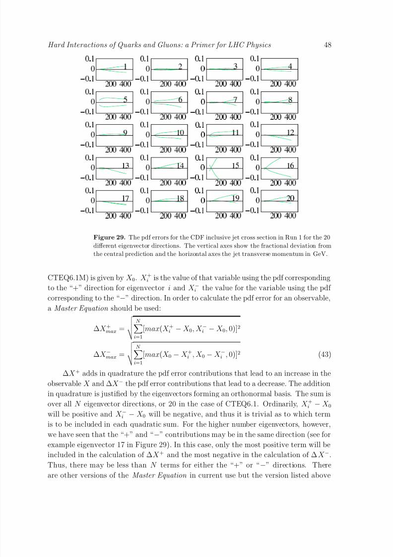
8/3/2019 Hard Interactions of Quarks and Gluons a Primer for LHC Physics
http://slidepdf.com/reader/full/hard-interactions-of-quarks-and-gluons-a-primer-for-lhc-physics 48/118
Hard Interactions of Quarks and Gluons: a Primer for LHC Physics 48
Figure 29. The pdf errors for the CDF inclusive jet cross section in Run 1 for the 20
different eigenvector directions. The vertical axes show the fractional deviation from
the central prediction and the horizontal axes the jet transverse momentum in GeV.
CTEQ6.1M) is given by X 0. X +i is the value of that variable using the pdf corresponding
to the “+” direction for eigenvector i and X −i
the value for the variable using the pdf
corresponding to the “−” direction. In order to calculate the pdf error for an observable,
a Master Equation should be used:
∆X +max =
N i=1
[max(X +i − X 0, X −i − X 0, 0)]2
∆X −max =
N i=1
[max(X 0 − X +i , X 0 − X −i , 0)]2 (43)
∆X + adds in quadrature the pdf error contributions that lead to an increase in the
observable X and ∆X − the pdf error contributions that lead to a decrease. The addition
in quadrature is justified by the eigenvectors forming an orthonormal basis. The sum is
over all N eigenvector directions, or 20 in the case of CTEQ6.1. Ordinarily, X +i − X 0will be positive and X −i − X 0 will be negative, and thus it is trivial as to which term
is to be included in each quadratic sum. For the higher number eigenvectors, however,
we have seen that the “+” and “−” contributions may be in the same direction (see for
example eigenvector 17 in Figure 29). In this case, only the most positive term will be
included in the calculation of ∆X + and the most negative in the calculation of ∆X −.
Thus, there may be less than N terms for either the “+” or “−” directions. There
are other versions of the Master Equation in current use but the version listed above

8/3/2019 Hard Interactions of Quarks and Gluons a Primer for LHC Physics
http://slidepdf.com/reader/full/hard-interactions-of-quarks-and-gluons-a-primer-for-lhc-physics 49/118
Hard Interactions of Quarks and Gluons: a Primer for LHC Physics 49
is the “official” recommendation of the authors. Either X 0 and X ±i can be calculated
separately in a matrix element/Monte Carlo program (requiring the program to be run
2N + 1 times) or X 0 can be calculated with the program and at the same time the
ratio of the pdf luminosities (the product of the two pdfs at the x values used in the
generation of the event) for eigenvector i (±) to that of the central fit can be calculated
and stored. This results in an effective sample with 2N + 1 weights, but identical
kinematics, requiring a substantially reduced amount of time to generate.
Perhaps the most controversial aspect of pdf uncertainties is the determination
of the ∆χ2 excursion from the central fit that is representative of a reasonable error.
CTEQ chooses a ∆χ2 value of 100 (corresponding to a 90% CL limit) while MRST
uses a value of 50. Thus, in general, the pdf uncertainties for any cross section will
be larger for the CTEQ set than for the MRST set. The difference in the criterion
indicates the difficulty of treating the error analysis for such a large disparate sample
of data in a statistically rigorous and unique manner. But in any case, both groups arein agreement that a χ2 excursion of 1 (for a 1σ error) is too low of a value in a global
pdf fit. The global fits use data sets arising from a number of different processes and
different experiments; there is a non-negligible tension between some of the different
data sets. pdf fits performed within a single experiment, or with a single data type may
be able to set tighter tolerances. The uncertainties for all predictions should be linearly
dependent on the tolerance parameter used; thus, it should be reasonable to scale the
uncertainty for an observable from the 90% CL limit provided by the CTEQ/MRST
error pdfs to a one-sigma error by dividing by a factor of 1 .6. Such a scaling will be a
better approximation for observables more dependent on the low number eigenvectors,
where the χ2 function is closer to a quadratic form. Note that such a scaling may resultin an underestimate of the true pdf uncertainty, as the central results for CTEQ and
MRST often differ by an amount similar to this one-sigma error. (See the discussion in
Section 2.2 regarding the W cross section predictions at the Tevatron.)
The CTEQ and MRST uncertainties for the up quark and gluon distributions are
shown in Figures 30, 31, 32 and 33. The pdf luminosity uncertainties for various pdf
combinations for some kinematic situations appropriate to the LHC will be discussed in
Section 6.
Both the CTEQ and MRST groups typically use a fixed value of αS (M 2Z ) (equal
to the PDG world average [119] in their global fits. An additional uncertainty in thedetermination of pdfs results from the uncertainty in the value of αS (M 2Z ) used in the
global fits. Figure 34 and Figure 35 show the results of varying the value of αS on
the gluon and up quark distributions [120]. As expected, the gluon distribution has a
greater sensitivity on αS due to the coupling mentioned earlier.
4.5. NLO and LO pdfs
In the past, the global pdf fitting groups have produced sets of pdfs in which leading
order rather than next-to-leading order matrix elements, along with the 1-loop αS rather
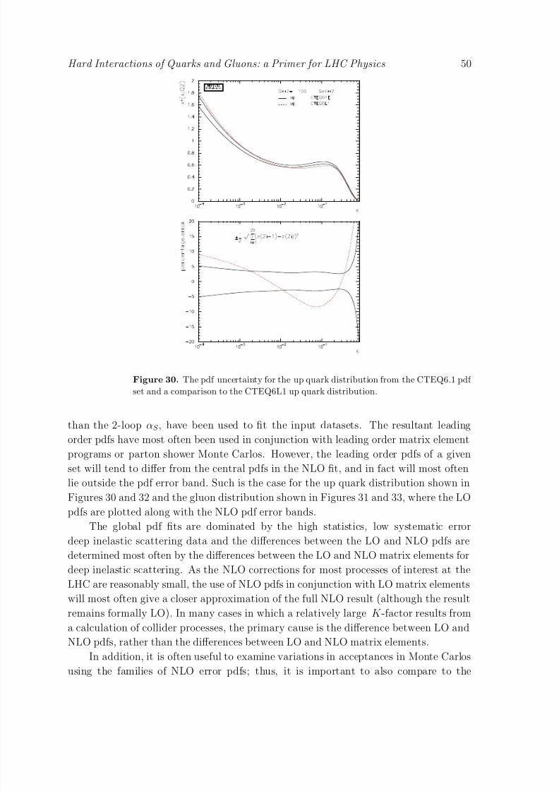
8/3/2019 Hard Interactions of Quarks and Gluons a Primer for LHC Physics
http://slidepdf.com/reader/full/hard-interactions-of-quarks-and-gluons-a-primer-for-lhc-physics 50/118
Hard Interactions of Quarks and Gluons: a Primer for LHC Physics 50
Figure 30. The pdf uncertainty for the up quark distribution from the CTEQ6.1 pdf
set and a comparison to the CTEQ6L1 up quark distribution.
than the 2-loop αS , have been used to fit the input datasets. The resultant leading
order pdfs have most often been used in conjunction with leading order matrix element
programs or parton shower Monte Carlos. However, the leading order pdfs of a given
set will tend to differ from the central pdfs in the NLO fit, and in fact will most often
lie outside the pdf error band. Such is the case for the up quark distribution shown in
Figures 30 and 32 and the gluon distribution shown in Figures 31 and 33, where the LO
pdfs are plotted along with the NLO pdf error bands.
The global pdf fits are dominated by the high statistics, low systematic error
deep inelastic scattering data and the differences between the LO and NLO pdfs are
determined most often by the differences between the LO and NLO matrix elements fordeep inelastic scattering. As the NLO corrections for most processes of interest at the
LHC are reasonably small, the use of NLO pdfs in conjunction with LO matrix elements
will most often give a closer approximation of the full NLO result (although the result
remains formally LO). In many cases in which a relatively large K -factor results from
a calculation of collider processes, the primary cause is the difference between LO and
NLO pdfs, rather than the differences between LO and NLO matrix elements.
In addition, it is often useful to examine variations in acceptances in Monte Carlos
using the families of NLO error pdfs; thus, it is important to also compare to the
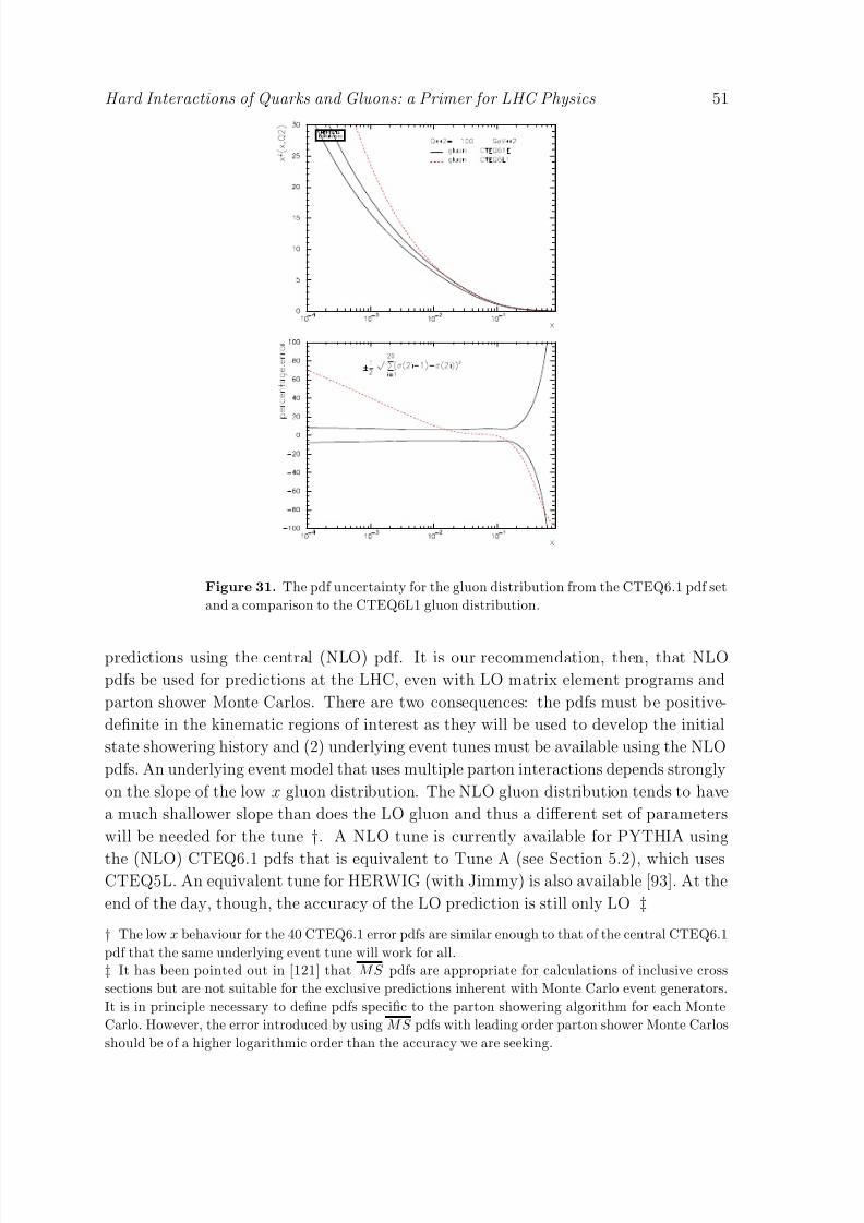
8/3/2019 Hard Interactions of Quarks and Gluons a Primer for LHC Physics
http://slidepdf.com/reader/full/hard-interactions-of-quarks-and-gluons-a-primer-for-lhc-physics 51/118
Hard Interactions of Quarks and Gluons: a Primer for LHC Physics 51
Figure 31. The pdf uncertainty for the gluon distribution from the CTEQ6.1 pdf set
and a comparison to the CTEQ6L1 gluon distribution.
predictions using the central (NLO) pdf. It is our recommendation, then, that NLO
pdfs be used for predictions at the LHC, even with LO matrix element programs and
parton shower Monte Carlos. There are two consequences: the pdfs must be positive-
definite in the kinematic regions of interest as they will be used to develop the initial
state showering history and (2) underlying event tunes must be available using the NLO
pdfs. An underlying event model that uses multiple parton interactions depends strongly
on the slope of the low x gluon distribution. The NLO gluon distribution tends to have
a much shallower slope than does the LO gluon and thus a different set of parameters
will be needed for the tune
†. A NLO tune is currently available for PYTHIA using
the (NLO) CTEQ6.1 pdfs that is equivalent to Tune A (see Section 5.2), which usesCTEQ5L. An equivalent tune for HERWIG (with Jimmy) is also available [93]. At the
end of the day, though, the accuracy of the LO prediction is still only LO ‡† The low x behaviour for the 40 CTEQ6.1 error pdfs are similar enough to that of the central CTEQ6.1
pdf that the same underlying event tune will work for all.
‡ It has been pointed out in [121] that MS pdfs are appropriate for calculations of inclusive cross
sections but are not suitable for the exclusive predictions inherent with Monte Carlo event generators.
It is in principle necessary to define pdfs specific to the parton showering algorithm for each Monte
Carlo. However, the error introduced by using M S pdfs with leading order parton shower Monte Carlos
should be of a higher logarithmic order than the accuracy we are seeking.

8/3/2019 Hard Interactions of Quarks and Gluons a Primer for LHC Physics
http://slidepdf.com/reader/full/hard-interactions-of-quarks-and-gluons-a-primer-for-lhc-physics 52/118
Hard Interactions of Quarks and Gluons: a Primer for LHC Physics 52
Figure 32. The pdf uncertainty for the up quark distribution from the MRST2001
pdf set and a comparison to the MRST2001LO up quark distribution.
The transition from NLO to NNLO results in much smaller changes to the pdfs as
can be observed in Figure 36.
4.6. Pdf uncertainties and Sudakov form factors
As discussed in the above section, it is often useful to use the error pdf sets with parton
shower Monte Carlos. The caveat still remains that a true test of the acceptances would
use a NLO MC. Similar to their use with matrix element calculations, events can be
generated once using the central pdf and the pdf weights stored for the error pdfs.
These pdf weights then can be used to construct the pdf uncertainty for any observable.Some sample code for PYTHIA is given on the benchmark website. One additional
complication with respect to their use in matrix element programs is that the parton
distributions are used to construct the initial state parton showers through the backward
evolution process. The space-like evolution of the initial state partons is guided by the
ratio of parton distribution functions at different x and Q2 values, c.f. (41). Thus the
Sudakov form factors in parton shower Monte Carlos will be constructed using only the
central pdf and not with any of the individual error pdfs and this may lead to some
errors for the calculation of the pdf uncertainties of some observables. However, it was
demonstrated in Reference [86] that the pdf uncertainty for Sudakov form factors in the

8/3/2019 Hard Interactions of Quarks and Gluons a Primer for LHC Physics
http://slidepdf.com/reader/full/hard-interactions-of-quarks-and-gluons-a-primer-for-lhc-physics 53/118
Hard Interactions of Quarks and Gluons: a Primer for LHC Physics 53
Figure 33. The pdf uncertainty for the gluon distribution from the MRST2001 pdf
set and a comparison to the MRST2001LO gluon distribution.
kinematic region relevant for the LHC is minimal, and the weighting technique can be
used just as well with parton shower Monte Carlos as with matrix element programs.
4.7. LHAPDF
Libraries such as PDFLIB [122] have been established that maintain a large collection
of available pdfs. However, PDFLIB is no longer supported, making it more difficult
for easy access to the most up-to-date pdfs. In addition, the determination of the pdf
uncertainty of any cross section typically involves the use of a large number of pdfs (on
the order of 30-100) and PDFLIB is not set up for easy accessibility for a large numberof pdfs.
At Les Houches in 2001, representatives from a number of pdf groups were present
and an interface (Les Houches Accord 2, or LHAPDF) [124] that allows the compact
storage of the information needed to define a pdf was defined. Each pdf can be
determined either from a grid in x and Q2 or by a few lines of information (basically the
starting values of the parameters at Q = Qo) and the interface carries out the evolution
to any x and Q value, at either LO or NLO as appropriate for each pdf.
The interface is as easy to use as PDFLIB and consists essentially of 3 subroutine
calls:

8/3/2019 Hard Interactions of Quarks and Gluons a Primer for LHC Physics
http://slidepdf.com/reader/full/hard-interactions-of-quarks-and-gluons-a-primer-for-lhc-physics 54/118
Hard Interactions of Quarks and Gluons: a Primer for LHC Physics 54
Figure 34. Variation of the up quark distribution for different values of αS. αS varies
from 0.110 (short-dash) to 0.124 (long-dash) in increments of 0.002.
•call Initpdfset(name): called once at the beginning of the code; name is the file name
of the external pdf file that defines the pdf set (for example, CTEQ, GKK [123] or
MRST)
• call Initpdf(mem ): mem specifies the individual member of the pdf set
• call evolvepdf(x,Q,f ): returns the pdf momentum densities for flavour f at a
momentum fraction x and scale Q
Responsibility for LHAPDF has been taken over by the Durham HEPDATA
project [125] and regular updates/improvements have been produced. It is currently
included in the matrix element program MCFM [126] and will be included in future
versions of other matrix element and parton shower Monte Carlo programs. Recentmodifications make it possible to include all error pdfs in memory at the same time.
Such a possibility reduces the amount of time needed for pdf error calculations on any
observable. The matrix element result can be calculated once using the central pdf and
the relative (pdf)×(pdf) parton-parton luminosity can be calculated for each of the error
pdfs (or the values of x1,x2, the flavour of partons 1 and 2 and the value of Q2 can be
stored). Such a pdf re-weighting has been shown to work both for exact matrix element
calculations as well as for matrix element+parton shower calculations. In addition, a
new routine LHAGLUE [125] provides an interface from PDFLIB to LHAPDF making
it possible to use the PDFLIB subroutine calls that may be present in older programs.

8/3/2019 Hard Interactions of Quarks and Gluons a Primer for LHC Physics
http://slidepdf.com/reader/full/hard-interactions-of-quarks-and-gluons-a-primer-for-lhc-physics 55/118
Hard Interactions of Quarks and Gluons: a Primer for LHC Physics 55
Figure 35. Variation of the gluon distribution for different values of αS. αS varies
from 0.110 (short-dash) to 0.124 (long-dash) in increments of 0.002.
Figure 36. A comparison of the NLO and NNLO gluon and up quark distributions
for the MRST2004 sets of pdfs.
5. Comparisons to Tevatron data
5.1. W / Z production
As discussed earlier, W production at hadron-hadron colliders serves as a precision
benchmark for Standard Model physics. Experimentally, the systematic errors are small.

8/3/2019 Hard Interactions of Quarks and Gluons a Primer for LHC Physics
http://slidepdf.com/reader/full/hard-interactions-of-quarks-and-gluons-a-primer-for-lhc-physics 56/118
Hard Interactions of Quarks and Gluons: a Primer for LHC Physics 56
The decay leptons are easy to trigger on and the backgrounds are under good control.
Theoretically, the cross section and rapidity distributions are known to NNLO. The W
and Z cross sections measured at the Tevatron are shown in Figure 37 for both Run 1 and
Run 2 [12]. The experimental cross sections agree well with the predictions and the Run
2 cross sections show the rise expected from the increase in centre-of-mass energy over
Run 1. In Figure 4 in Section 2, the Run 2 cross sections from CDF and D0 are compared
to predictions at LO, NLO and NNLO. The NNLO predictions are a few percent larger
than the NLO predictions. Good agreement is observed with both. It is noteworthy that
the largest experimental uncertainty for the W and Z cross sections is the uncertainty
in the luminosity, typically on the order of 5%. The theoretical systematic errors are
primarily from the pdf uncertainty. If other Tevatron cross sections were normalized to
the W cross section, then both the theoretical and experimental systematic errors for
those cross sections could be reduced.
Predictions of the rapidity distribution for Z (→ e+
e−
) production at the Tevatronare shown in Figure 38 [68, 129]. There is a shape change in going from LO to NLO,
as well as an increase in normalization, while the transition from NLO to NNLO is
essentially just a small K -factor with little change in shape. The Z rapidity distribution
measured by D0 in Run 2 is shown in Figure 39 [13]; the measurement agrees with the
NNLO prediction over the entire rapidity range. Such cross sections may be useful as
input to global pdf fits in the near future.
The transverse momentum distribution for Z bosons at the Tevatron (CDF Run
1) is shown in Figures 40 (low pT ) and 41 (all pT ) along with comparisons to the
parton showers PYTHIA and ResBos which are discussed in Section 3.5. The ResBos
predictions agree well with the data over the entire kinematic region, while the PYTHIApredictions require the addition of an intrinsic kT of approximately 2 GeV for best
agreement at lower transverse momentum. This intrinsic kT is not totally due to the
finite size of the proton; it mostly results from the finite cutoff in the parton shower
evolution and the need to add the missing component back “by-hand”. ResBos correctly
10-1
1
0.4 0.6 0.8 1 1.2 1.4 1.6 1.8 2E
cm(TeV)
σ
×
B r ( n b )
σ×Br(W→l ν)
σ×Br(Z→l+l-)
CDF II (e+µ)
CDF I (e)
DO I (e)
CDF (630)
UA1 (µ)
UA2 (e)theory curves:
Martin, Roberts, Stirling, Thorne
Figure 37. W and Z cross sections as a function of the centre-of-mass energy.

8/3/2019 Hard Interactions of Quarks and Gluons a Primer for LHC Physics
http://slidepdf.com/reader/full/hard-interactions-of-quarks-and-gluons-a-primer-for-lhc-physics 57/118
Hard Interactions of Quarks and Gluons: a Primer for LHC Physics 57
Figure 38. Predictions for the rapidity distribution of an on-shell Z boson in Run
2 at the Tevatron at LO, NLO and NNLO. The bands indicate the variation of the
renormalization and factorization scales within the range M Z/2 to 2M Z .
Y(Z)-3 -2 -1 0 1 2 3
/ d Y
σ
d
σ
1 /
0
0.05
0.1
0.15
0.2
0.25
0.3
Rapidity*γ Z/
NNLO, MRST01Data
Run II Preliminary∅D
Figure 39. Z rapidity distribution from D0 in Run 2.
describes the non-perturbative as well as the perturbative region.
The average transverse momentum for Drell-Yan production has been measured as
a function of the Drell-Yan pair mass in CDF in Run 2. This is shown in Figure 42 [127].
The average transverse momentum (neglecting the high pT tail) increases roughly
logarithmically with the square of the Drell-Yan mass. The data agree well with the
default PYTHIA 6.2 prediction using Tune A. Also shown are two predictions involving
tunes of PYTHIA that give larger/smaller values for the average Drell-Yan transverse
momentum as a function of the Drell-Yan mass. The Plus/Minus tunes were used to
estimate the initial-state-radiation uncertainty for the determination of the top mass in
CDF. Most of the tt cross section at the Tevatron arises from qq initial states, so the
Drell-Yan measurements serve as a good model. (See further discussion in Section 5.5.)

8/3/2019 Hard Interactions of Quarks and Gluons a Primer for LHC Physics
http://slidepdf.com/reader/full/hard-interactions-of-quarks-and-gluons-a-primer-for-lhc-physics 58/118
Hard Interactions of Quarks and Gluons: a Primer for LHC Physics 58
Figure 40. The transverse momentum distribution (low pT ) for Z → e+e− from
CDF in Run 1, along with comparisons to predictions from PYTHIA and ResBos.
The dashed-blue curve is the default PYTHIA prediction. The PYTHIA solid-green
curve has had an additional 2 GeV of kT added to the parton shower.
Figure 41. The transverse momentum distribution (full pT range) for Z → e+e− from
CDF in Run 1, along with comparisons to predictions from PYTHIA (solid histogram)
and ResBos.
The information regarding these tunes is available on the benchmarks website.
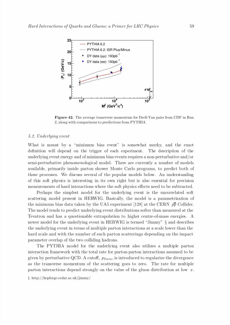
8/3/2019 Hard Interactions of Quarks and Gluons a Primer for LHC Physics
http://slidepdf.com/reader/full/hard-interactions-of-quarks-and-gluons-a-primer-for-lhc-physics 59/118
Hard Interactions of Quarks and Gluons: a Primer for LHC Physics 59
)4/c2
(GeV2M
310
410
510
( G e V / c )
⟩ T
P ⟨
0
5
10
15
20
25
2
top4*M
PYTHIA 6.2
PYTHIA 6.2: ISR Plus/Minus-1
): 193pbµµDY data (-1
DY data (ee): 193pb
Figure 42. The average transverse momentum for Drell-Yan pairs from CDF in Run
2, along with comparisons to predictions from PYTHIA.
5.2. Underlying event
What is meant by a “minimum bias event” is somewhat murky, and the exact
definition will depend on the trigger of each experiment. The description of the
underlying event energy and of minimum bias events requires a non-perturbative and/or
semi-perturbative phenomenological model. There are currently a number of models
available, primarily inside parton shower Monte Carlo programs, to predict both of these processes. We discuss several of the popular models below. An understanding
of this soft physics is interesting in its own right but is also essential for precision
measurements of hard interactions where the soft physics effects need to be subtracted.
Perhaps the simplest model for the underlying event is the uncorrelated soft
scattering model present in HERWIG. Basically, the model is a parametrization of
the minimum bias data taken by the UA5 experiment [128] at the CERN pp Collider.
The model tends to predict underlying event distributions softer than measured at the
Tevatron and has a questionable extrapolation to higher centre-of-mass energies. A
newer model for the underlying event in HERWIG is termed “Jimmy”
§and describes
the underlying event in terms of multiple parton interactions at a scale lower than thehard scale and with the number of such parton scatterings depending on the impact
parameter overlap of the two colliding hadrons.
The PYTHIA model for the underlying event also utilizes a multiple parton
interaction framework with the total rate for parton-parton interactions assumed to be
given by perturbative QCD. A cutoff, pTmin, is introduced to regularize the divergence
as the transverse momentum of the scattering goes to zero. The rate for multiple
parton interactions depend strongly on the value of the gluon distribution at low x.
§ http://hepforge.cedar.ac.uk/jimmy/
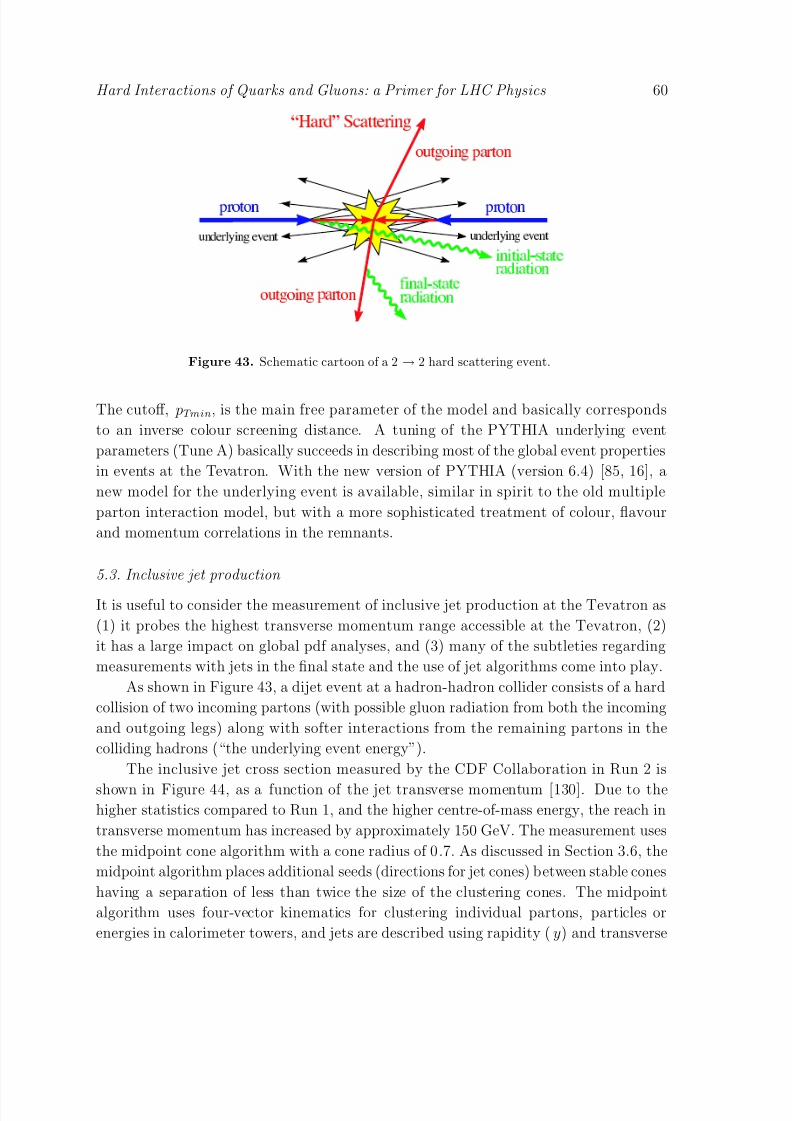
8/3/2019 Hard Interactions of Quarks and Gluons a Primer for LHC Physics
http://slidepdf.com/reader/full/hard-interactions-of-quarks-and-gluons-a-primer-for-lhc-physics 60/118
Hard Interactions of Quarks and Gluons: a Primer for LHC Physics 60
Figure 43. Schematic cartoon of a 2 → 2 hard scattering event.
The cutoff, pTmin, is the main free parameter of the model and basically corresponds
to an inverse colour screening distance. A tuning of the PYTHIA underlying event
parameters (Tune A) basically succeeds in describing most of the global event properties
in events at the Tevatron. With the new version of PYTHIA (version 6.4) [85, 16], a
new model for the underlying event is available, similar in spirit to the old multiple
parton interaction model, but with a more sophisticated treatment of colour, flavour
and momentum correlations in the remnants.
5.3. Inclusive jet production
It is useful to consider the measurement of inclusive jet production at the Tevatron as
(1) it probes the highest transverse momentum range accessible at the Tevatron, (2)
it has a large impact on global pdf analyses, and (3) many of the subtleties regarding
measurements with jets in the final state and the use of jet algorithms come into play.
As shown in Figure 43, a dijet event at a hadron-hadron collider consists of a hard
collision of two incoming partons (with possible gluon radiation from both the incoming
and outgoing legs) along with softer interactions from the remaining partons in the
colliding hadrons (“the underlying event energy”).
The inclusive jet cross section measured by the CDF Collaboration in Run 2 is
shown in Figure 44, as a function of the jet transverse momentum [130]. Due to thehigher statistics compared to Run 1, and the higher centre-of-mass energy, the reach in
transverse momentum has increased by approximately 150 GeV. The measurement uses
the midpoint cone algorithm with a cone radius of 0.7. As discussed in Section 3.6, the
midpoint algorithm places additional seeds (directions for jet cones) between stable cones
having a separation of less than twice the size of the clustering cones. The midpoint
algorithm uses four-vector kinematics for clustering individual partons, particles or
energies in calorimeter towers, and jets are described using rapidity (y) and transverse

8/3/2019 Hard Interactions of Quarks and Gluons a Primer for LHC Physics
http://slidepdf.com/reader/full/hard-interactions-of-quarks-and-gluons-a-primer-for-lhc-physics 61/118
Hard Interactions of Quarks and Gluons: a Primer for LHC Physics 61
(GeV/c)JetTP
0 100 200 300 400 500 600 700
( G e V / c )
n b
T
d Y d P σ
2 d
-810
-710
-610
-510
-410
-310
-210
-110
1
10
210
CDF Run II Preliminary
0.1<|Y|<0.7
-1
L=1.04 fb∫
=1.3)Sep
=0.75, Rmerge
=0.7, fcone
Midpoint (R
Systematic uncertainty
Data corrected to hadron level
/2)Jet
T=PµNLO pQCD EKS CTEQ 6.1M (
Figure 44. The inclusive jet cross section from CDF in Run 2.
momentum ( pT ) .
5.3.1. Corrections For comparison of data to theory, the calorimeter tower energies
clustered into a jet must first be corrected for the detector response. The calorimeters
in the CDF experiment respond differently to electromagnetic showers than to hadronic
showers, and the difference varies as a function of the transverse momentum of the jet. The detector response corrections are determined using a detector simulation
in which the parameters have been tuned to test-beam and in-situ calorimeter data.
PYTHIA 6.216, with Tune A, is used for the production and fragmentation of jets.
The same clustering procedure is applied to the final state particles in PYTHIA as is
done for the data. The correction is determined by matching the calorimeter jet to the
corresponding particle jet. An additional correction accounts for the smearing effects
due to the finite energy resolution of the calorimeter. At this point, the jet is said to be
determined at the “hadron level.”
For data to be compared to a parton level calculation, either the data must becorrected from the hadron level to the parton level or the theory must be corrected to the
hadron level. Here we describe the former; the latter just involves the inverse corrections.
It is our “official recommendation” that, where possible, the data be presented at least at
the hadron level, and the corrections between hadron and parton level be clearly stated.
The hadronization corrections consist of two components: the subtraction from the jet
of the underlying event energy not associated with the hard scattering and the correction
for a loss of energy outside a jet due to the fragmentation process. The hadronization
Self-contained versions of the CDF midpoint cone algorithm, as well as the Run 1 cone algorithm
JetClu, are available at the benchmark website, in both Fortran and C++ versions
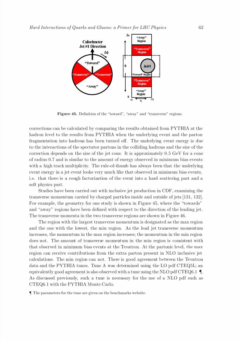
8/3/2019 Hard Interactions of Quarks and Gluons a Primer for LHC Physics
http://slidepdf.com/reader/full/hard-interactions-of-quarks-and-gluons-a-primer-for-lhc-physics 62/118
Hard Interactions of Quarks and Gluons: a Primer for LHC Physics 62
Figure 45. Definition of the “toward”, “away” and “transverse” regions.
corrections can be calculated by comparing the results obtained from PYTHIA at the
hadron level to the results from PYTHIA when the underlying event and the parton
fragmentation into hadrons has been turned off. The underlying event energy is due
to the interactions of the spectator partons in the colliding hadrons and the size of the
correction depends on the size of the jet cone. It is approximately 0.5 GeV for a cone
of radius 0.7 and is similar to the amount of energy observed in minimum bias events
with a high track multiplicity. The rule-of-thumb has always been that the underlying
event energy in a jet event looks very much like that observed in minimum bias events,
i.e. that there is a rough factorization of the event into a hard scattering part and asoft physics part.
Studies have been carried out with inclusive jet production in CDF, examining the
transverse momentum carried by charged particles inside and outside of jets [131, 132].
For example, the geometry for one study is shown in Figure 45, where the “towards”
and “away” regions have been defined with respect to the direction of the leading jet.
The transverse momenta in the two transverse regions are shown in Figure 46.
The region with the largest transverse momentum is designated as the max region
and the one with the lowest, the min region. As the lead jet transverse momentum
increases, the momentum in the max region increases; the momentum in the min region
does not. The amount of transverse momentum in the min region is consistent withthat observed in minimum bias events at the Tevatron. At the partonic level, the max
region can receive contributions from the extra parton present in NLO inclusive jet
calculations. The min region can not. There is good agreement between the Tevatron
data and the PYTHIA tunes. Tune A was determined using the LO pdf CTEQ5L; an
equivalently good agreement is also observed with a tune using the NLO pdf CTEQ6.1 ¶.
As discussed previously, such a tune is necessary for the use of a NLO pdf such as
CTEQ6.1 with the PYTHIA Monte Carlo.
¶ The parameters for the tune are given on the benchmarks website.

8/3/2019 Hard Interactions of Quarks and Gluons a Primer for LHC Physics
http://slidepdf.com/reader/full/hard-interactions-of-quarks-and-gluons-a-primer-for-lhc-physics 63/118
Hard Interactions of Quarks and Gluons: a Primer for LHC Physics 63
Figure 46. The sum of the transverse momenta of charged particles inside the
TransMAX and TransMIN regions, as a function of the transverse momentum of the
leading jet.
The jet shape is also well described by PYTHIA predictions using Tune A, as can
be seen in Figure 47 [134], where the jet energy away from the core of the jet (i.e. in
the annulus from 0.3 to 0.7) is plotted as a function of the transverse momentum of
the jet. A better description is provided by the use of Tune A then with the default
PYTHIA prediction. A reasonable description of the core of the jet (< 0.3) can also beprovided by the pure NLO prediction [14]. Jets become more collimated as the inclusive
jet transverse momentum increases for three reasons: (1)) power corrections that tend
to broaden the jet decrease as 1/pT or 1/p2T , (2) a larger fraction of jets are quark
jets rather than gluon jets and (3), the probability of a hard gluon to be radiated (the
dominant factor in the jet shape) decreases as αS ( p2T ).
The fragmentation correction accounts for the daughter hadrons ending up outside
the jet cone from mother partons whose trajectories lie inside the cone (also known
as splash-out ); it does not correct for any out-of-cone energy arising from perturbative
effects as these should be correctly accounted for in a NLO calculation. It is purely a
power correction to the cross section. The numerical value of the splash-out energy isroughly constant at 1 GeV for a cone of radius 0.7, independent of the jet transverse
momentum. This constancy may seems surprising. But, as the jet transverse momentum
increases, the jet becomes more collimated; the result is that the energy in the outermost
annulus (the origin of the splash-out energy) is roughly constant. The correction for
splash-out derived using parton shower Monte Carlos can be applied to a NLO parton
level calculation to the extent to which both the parton shower and the 2 partons in a
NLO jet correctly describe the jet shape.
The two effects (underlying event and splash-out) go in opposite directions so there
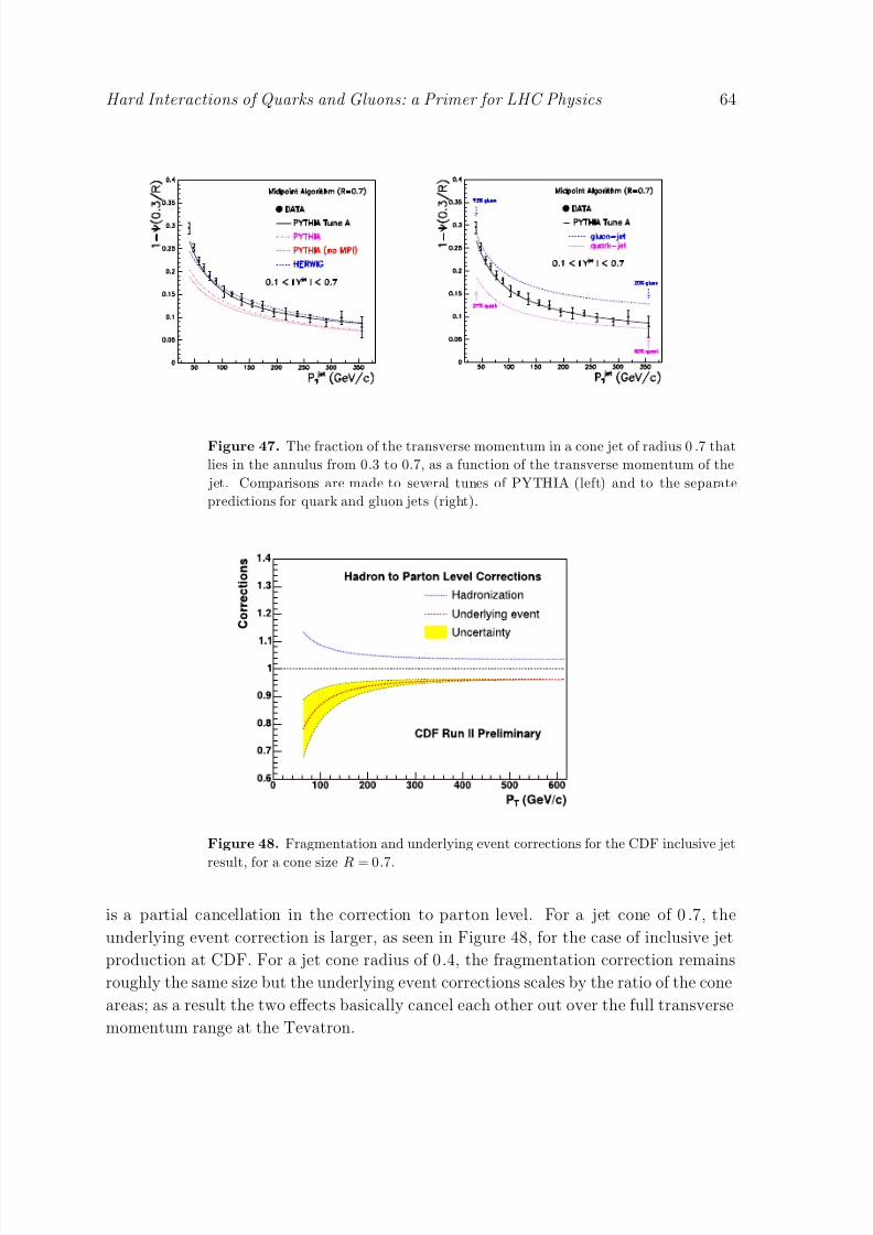
8/3/2019 Hard Interactions of Quarks and Gluons a Primer for LHC Physics
http://slidepdf.com/reader/full/hard-interactions-of-quarks-and-gluons-a-primer-for-lhc-physics 64/118
Hard Interactions of Quarks and Gluons: a Primer for LHC Physics 64
Figure 47. The fraction of the transverse momentum in a cone jet of radius 0 .7 that
lies in the annulus from 0.3 to 0.7, as a function of the transverse momentum of the
jet. Comparisons are made to several tunes of PYTHIA (left) and to the separate
predictions for quark and gluon jets (right).
Figure 48. Fragmentation and underlying event corrections for the CDF inclusive jet
result, for a cone size R = 0.7.
is a partial cancellation in the correction to parton level. For a jet cone of 0.7, the
underlying event correction is larger, as seen in Figure 48, for the case of inclusive jet
production at CDF. For a jet cone radius of 0.4, the fragmentation correction remains
roughly the same size but the underlying event corrections scales by the ratio of the cone
areas; as a result the two effects basically cancel each other out over the full transverse
momentum range at the Tevatron.

8/3/2019 Hard Interactions of Quarks and Gluons a Primer for LHC Physics
http://slidepdf.com/reader/full/hard-interactions-of-quarks-and-gluons-a-primer-for-lhc-physics 65/118
Hard Interactions of Quarks and Gluons: a Primer for LHC Physics 65
(GeV/c)Jet
TP
0 100 200 300 400 500 600 700
C r o s s S e c t i o n R a t i o ( D a t a / T
h e o r y )
0.5
1
1.5
2
2.5
3 Data corrected to the parton level
/2)Jet
T
=PµNLO pQCD EKS CTEQ 6.1M (
=1.3)Sep
=0.75, Rmerge
=0.7, fcone
Midpoint (R
-1
L=1.04 fb∫ 0.1<|Y|<0.7
PDF uncertainty on pQCD
MRST 2004 / CTEQ 6.1MData / NLO pQCDSystematic uncertainty
Systematic uncertainty including
hadronization and UE
CDF Run II Preliminary
Figure 49. The inclusive jet cross section from CDF in Run 2 compared on a linear
scale to NLO theoretical predictions using CTEQ6.1 and MRST2004 pdfs.
5.3.2. Results A comparison of the inclusive jet cross section measured by CDF in
Run 2 with the midpoint cone algorithm [135] to NLO pQCD predictions using theEKS [133] program with the CTEQ6.1 and MRST2004 pdfs is shown in Figure 49.
A renormalization/factorization scale of ( p jetT /2) has been used in the calculation.
Typically, this leads to the highest predictions for inclusive jet cross sections at the
Tevatron, as discussed in Section 3.3.2. There is good agreement with the CTEQ6.1
predictions over the transverse momentum range of the prediction. The MRST2004
predictions are slightly higher at lower pT and slightly lower at higher pT , but still
in good overall agreement. As noted before, the CTEQ6.1 and MRST2004 pdfs have a
higher gluon at large x as compared to previous pdfs, due to the influence of the Run 1 jet
data from CDF and D0. This enhanced gluon provides a good agreement with the high
pT Run 2 measurement as well which, as stated before, extends approximately 150 GeVhigher in transverse momentum. The red curves indicate the pdf uncertainty for the
prediction using the CTEQ6.1 pdf error set. The yellow band indicates the experimental
systematic uncertainty, which is dominated by the uncertainty in the jet energy scale
(on the order of 3%). The purple band shows the effect of the uncertainty due to the
hadronization and underlying event, which is visible only for transverse momenta below
100 GeV. In Figure 50, the jet cross sections measured with the midpoint cone algorithm
are shown for the full rapidity coverage of the CDF experiment. Good agreement is
observed in all rapidity regions with the CTEQ6.1 predictions. It is also important to

8/3/2019 Hard Interactions of Quarks and Gluons a Primer for LHC Physics
http://slidepdf.com/reader/full/hard-interactions-of-quarks-and-gluons-a-primer-for-lhc-physics 66/118
Hard Interactions of Quarks and Gluons: a Primer for LHC Physics 66
D a t a / T h e o r y
0.5
1
1.5
2
2.5
3
3.5
|Y|<0.1 0.1<|Y|<0.7
D a t a / T h e o r y
0.5
1
1.5
2
2.5
3
3.5
0.7<|Y|<1.1
(GeV/c)JETTP
100 200 300 400 500 600 700
1.1<|Y|<1.6
(GeV/c)JETTP
0 100 200 300 400 500 600 700
D a t a
/ T h e o r y
0.5
1
1.52
2.5
3
3.5
1.6<|Y|<2.1PDF Uncertainty on pQCD
Data (parton level) / NLO pQCDSystematic uncertainty
Systematic uncertainty including
hadronization and UE
=0.75merge
=0.7, fcone
Midpoint R
=1.3sep
/2, RJET
T=PµNLO pQCD: EKS CTEQ 6.1M
CDF Run II Preliminary -1
L=1.04 fb∫
Figure 50. The inclusive jet cross section from CDF in Run 2, for several rapidity
intervals using the midpoint cone algorithm, compared on a linear scale to NLO
theoretical predictions using CTEQ6.1 pdfs.
note that for much of the kinematic range, the experimental systematic errors are lessthan pdf uncertainties; thus, the use of this data in future global pdf fits should serve
to further constrain the gluon pdf.
5.3.3. Jet algorithms and data For many events, the jet structure is clear and the jets
to which the individual towers should be assigned are fairly unambiguous. However, in
other events such as Figure 51, the complexity of the energy depositions means that
different algorithms will result in different assignments of towers to the various jets.
This is no problem to the extent that a similar complexity can be matched by the
theoretical calculation to which it is being compared. This is the case, for example,
for events simulated with parton shower Monte Carlos, but, as discussed in Section 3,current NLO calculations can place at most 2 partons in a jet.
In Figure 52, the experimental jet cross sections using the kT algorithm from
CDF Run 2 [136] are compared to NLO predictions using the JETRAD [88] program.
Similarly good agreement to that obtained for the midpoint cone algorithm is observed.
This is an important observation. The two different jet algorithms have different
strengths and weaknesses. It is our recommendation that, where possible, analyses
at the Tevatron and LHC use both algorithms in order to obtain more robust results.
We noted in Section 3.6 that on general principles, for NLO parton level predictions,

8/3/2019 Hard Interactions of Quarks and Gluons a Primer for LHC Physics
http://slidepdf.com/reader/full/hard-interactions-of-quarks-and-gluons-a-primer-for-lhc-physics 67/118
Hard Interactions of Quarks and Gluons: a Primer for LHC Physics 67
Figure 51. Impact of different jet clustering algorithms on an interesting event.
R a t i o t o C T E Q 6 . 1
M
1
2
3
|<0.1JET
|y |<0.7JET
0.1<|y
R a t i o t o C T E Q 6 . 1
M
1
2
3
|<1.1JET
0.7<|y
[GeV/c]JET
p
200 400 600
|<1.6JET
1.1<|y
[GeV/c]JETTp
0 200 400 600
R a t i o t o C T E Q 6 . 1
M
1
2
3
|<2.1JET
1.6<|y
[GeV/c]JETTp
D=0.7TK
)-1
Data ( L = 0.98 fbSystematic uncertaintiesPDF uncertainties
JETT
= max p0
µ= 2 xµMRST2004
CDF Run II Preliminary
Figure 52. The inclusive jet cross section from CDF in Run 2, for several rapidity
intervals using the kT jet algorithm, compared on a linear scale to NLO theoretical
predictions using CTEQ6.1 pdfs.
the cone jet cross section is larger than the kT jet cross section when Rcone = D. At
the hadron level, this is no longer true; the cone jet loses energy by the “splash-out”
effect while the kT algorithm has a tendency to “vacuum up” contributions from the

8/3/2019 Hard Interactions of Quarks and Gluons a Primer for LHC Physics
http://slidepdf.com/reader/full/hard-interactions-of-quarks-and-gluons-a-primer-for-lhc-physics 68/118
Hard Interactions of Quarks and Gluons: a Primer for LHC Physics 68
η
-3
-2
-1
0
1
2
3
φ
0
100
200
300
T E
0
5
10
Figure 53. An example of a Monte Carlo inclusive jet event where the midpoint
algorithm has left substantial energy unclustered.
underlying event. This will be corrected at least partially by the hadron to parton level
corrections for each algorithm.
A particular complexity with the cone algorithm occurs when two jets overlap; a
decision must be made whether to merge the two jets into one, or to separate them.
This is an experimental decision; in CDF in Run 2, the two overlapping jets are merged
when more than 75% of the smaller jet energy overlaps with the larger jet. When the
overlap is less, the towers are assigned to the nearest jet. D0 uses a criterion of a 50%
fraction. NLO theory is agnostic on the subject as there is no overlap between the two
partons that can comprise a jet. Further study is needed as to which choice is best,especially for the high luminosity conditions at the LHC.
Another problem that can arise on the particle or calorimeter level, but not on the
NLO parton level, occurs when particles or calorimeter towers remain unclustered in
any jet, due to the strong attraction of a nearby larger jet peak that will attract away
any trial jet cone placed at the location of the original particles/calorimeter towers.
The result will be what [89] calls “dark towers”, i.e. clusters that have a transverse
momentum large enough to be designated either a separate jet or to be included in an
existing nearby jet, but which are not clustered into either. Such a Monte Carlo event is
shown in Figure 53, where the towers unclustered into any jet are shaded black. A simple
way of understanding these dark towers begins by defining a “Snowmass potential” in
terms of the 2-dimensional vector −→r = (y, φ) via
V (−→r ) = −1
2
j
pT,j
R2
cone − (−→r j − −→r )2
Θ
R2cone − (−→r j − −→r )
2
. (44)
The flow is then driven by the “force”−→F (−→r ) = −−→∇V (−→r ) which is thus given by,
−→F (−→r ) =
j
pT,j (−→r j − −→r ) Θ
R2cone − (−→r j − −→r )2
=−→
rC (−→r ) − −→r
j⊂C (r)
pT,j , (45)
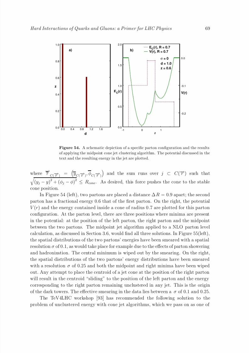
8/3/2019 Hard Interactions of Quarks and Gluons a Primer for LHC Physics
http://slidepdf.com/reader/full/hard-interactions-of-quarks-and-gluons-a-primer-for-lhc-physics 69/118
Hard Interactions of Quarks and Gluons: a Primer for LHC Physics 69
0.0 0.4 0.8 1.2 1.6
d
0.0
0.2
0.4
0.6
0.8
1.0
z
a)
-1 0 1
r
0.0
0.5
1.0
1.5
2.0
EC(r)
EC(r), R = 0.7
V(r), R = 0.7
σ = 0
-0.2
-0.1
0.0
V(r)
d = 1.0
z = 0.6
b)
Figure 54. A schematic depiction of a specific parton configuration and the results
of applying the midpoint cone jet clustering algorithm. The potential discussed in the
text and the resulting energy in the jet are plotted.
where−→r
C (−→r )
=
yC (
−→r ), φ
C (−→r )
and the sum runs over j ⊂ C (−→r ) such that
(y j−
y)2 + (φ j−
φ)2
≤Rcone. As desired, this force pushes the cone to the stable
cone position.
In Figure 54 (left), two partons are placed a distance ∆R = 0.9 apart; the second
parton has a fractional energy 0.6 that of the first parton. On the right, the potential
V (r) and the energy contained inside a cone of radius 0.7 are plotted for this parton
configuration. At the parton level, there are three positions where minima are present
in the potential: at the position of the left parton, the right parton and the midpoint
between the two partons. The midpoint jet algorithm applied to a NLO parton level
calculation, as discussed in Section 3.6, would find all three solutions. In Figure 55(left),
the spatial distributions of the two partons’ energies have been smeared with a spatial
resolution σ of 0.1, as would take place for example due to the effects of parton showeringand hadronization. The central minimum is wiped out by the smearing. On the right,
the spatial distributions of the two partons’ energy distributions have been smeared
with a resolution σ of 0.25 and both the midpoint and right minima have been wiped
out. Any attempt to place the centroid of a jet cone at the position of the right parton
will result in the centroid “sliding” to the position of the left parton and the energy
corresponding to the right parton remaining unclustered in any jet. This is the origin
of the dark towers. The effective smearing in the data lies between a σ of 0.1 and 0.25.
The TeV4LHC workshop [93] has recommended the following solution to the
problem of unclustered energy with cone jet algorithms, which we pass on as one of

8/3/2019 Hard Interactions of Quarks and Gluons a Primer for LHC Physics
http://slidepdf.com/reader/full/hard-interactions-of-quarks-and-gluons-a-primer-for-lhc-physics 70/118
Hard Interactions of Quarks and Gluons: a Primer for LHC Physics 70
-1.0 -0.5 0.0 0.5 1.0 1.5r
0.0
0.5
1.0
1.5
2.0
E C
( r )
EC(r), R = 0.7
V(r), R = 0.7σ = 0.1
a)
-0.20
-0.10
0.00
V ( r )
-1.0 -0.5 0.0 0.5 1.0 1.5
r
0.0
0.5
1.0
1.5
2.0
E C
( r )
EC(r), R = 0.7
V(r), R = 0.7σ = 0.25
b)
-0.2
-0.1
0.0
V ( r )
Figure 55. A schematic depiction of the effects of smearing on the midpoint cone jet
clustering algorithm.
our recommendations as well. The standard midpoint algorithm should be applied
to the list of calorimeter towers/particle/partons, including the full split/merge
procedure. The resulting identified jets are then referred to as first pass jets and their
towers/particles/partons are removed from the list. The same algorithm is then applied
to the remaining unclustered energy and any jets that result are referred to as second
pass jets. There are various possibilities for making use of the second pass jets. They
can be kept as separate jets, in addition to the first pass jets, or they can be merged
with the nearest first pass jets. The simplest solution, until further study, is to keepthe second pass jets as separate jets. This coding of this solution is available in the
midpoint algorithm given on the benchmark website.
It was originally thought that with the addition of a midpoint seed, the value
of Rsep used with the NLO theory could be returned to its natural value of 2.0(c.f.
Section 3.6). Now it is realized that the effects of parton showering/hadronization
result in the midpoint solution virtually always being lost. Thus, a value of Rsep of 1.3
is required for the NLO jet algorithm to best model the experimental one. The theory
cross section with Rsep = 1.3 is approximately 3 − 5% smaller than with Rsep = 2.0,
decreasing slowly with the jet transverse momentum.
5.3.4. Inclusive jet production at the Tevatron and global pdf fits Inclusive jet
production receives contributions from gg, gq and qq(qq) initial states as shown in
Figure 56 [11]. The experimental precision of the measurement, along with the remaining
theoretical uncertainties, means that the cross sections do not serve as a meaningful
constraint on the quark or antiquark distributions. However, they do serve as an
important constraint on the gluon distribution, especially at high x. Figure 57 shows
the gluon distributions for the CTEQ and MRST groups prior to the inclusion of any
inclusive jet data and the latest sets which include the Run 1 data from both CDF and

8/3/2019 Hard Interactions of Quarks and Gluons a Primer for LHC Physics
http://slidepdf.com/reader/full/hard-interactions-of-quarks-and-gluons-a-primer-for-lhc-physics 71/118
Hard Interactions of Quarks and Gluons: a Primer for LHC Physics 71
50 100 150 200 250 300 350 400 450 500
ET (GeV)
0
0.5
1
S u b p r o c e s s f r a c t i o n
p−
p −−> jet +X
√s = 1800 GeV CTEQ6M µ = ET /2 0< |η| <.5
CTEQ6M
CTEQ5M
qg
gg
Figure 56. The subprocess contributions to inclusive jet production at the Tevatron
for the CTEQ5M and CTEQ6M pdfs. The impact of the larger larger gluon at high x
for CTEQ6 is evident.
Figure 57. Gluon pdfs before and after the inclusion of Tevatron inclusive jet data.
D0. The influence of the high E T Run 1 jet cross section on the high x gluon is evident.
There is always the danger of sweeping new physics under the rug of pdf uncertainties.
Thus, it is important to measure the inclusive jet cross section over as wide a kinematic
range as possible. New physics tends to be central while a pdf explanation should be
universal, i.e. fit the data in all regions.

8/3/2019 Hard Interactions of Quarks and Gluons a Primer for LHC Physics
http://slidepdf.com/reader/full/hard-interactions-of-quarks-and-gluons-a-primer-for-lhc-physics 72/118
Hard Interactions of Quarks and Gluons: a Primer for LHC Physics 72
N Jets≥0 1 2 3 4
N J e t s ) [ p b ]
≥ ( σ
-210
-110
1
10
210
310
410
N Jets≥0 1 2 3 4
N J e t s ) [ p b ]
≥ ( σ
-210
-110
1
10
210
310
410
N Jets≥) +υe(W CDF Run II Preliminary
-1dL = 320 pb∫ CDF Data
W kin: 1.1≤|e
η20 [GeV]; |≥eTE
]2
20 [GeV/c≥W
T30 [GeV]; M≥ νTE
Jets: 2.0≤|jet
η15 [GeV]; |≥jet
TJetClu R=0.4; E
Hadron Level; no UE correction
MADGRAPH + PYTHIA CKKW
0 jets)≥(normalised to data
0 parton only
Up to 1 parton
Up to 2 partons
Up to 3 partons
Up to 4 partons
N Jets≥0 1 2 3 4
N J e t s ) [ p b ]
≥ ( σ
-110
1
10
210
310
N Jets≥) +υe(W CDF Run II Preliminary
-1dL = 320 pb∫ CDF Data
W kin: 1.1≤|e
η20 [GeV]; |≥eTE
]2
20 [GeV/c≥W
T30 [GeV]; M≥ νTE
Jets: 2.0≤|jet
η15 [GeV]; |≥jet
TJetClu R=0.4; E
Hadron Level; no UE correction
MCFM (parton level)
LO MADGRAPH + PYTHIA CKKW
Figure 58. The rate of production of W + n jets at CDF, compared to CKKW (left)
and also NLO QCD using MCFM (right). The measurements and predictions were
performed with a cone jet of radius 0.4 and with a requirement of 15 GeV or greater.
The CKKW predictions are normalized to the first bin and use a scale of 10 GeV for
the matching; the MCFM predictions are absolutely normalized.
5.4. W / Z + jets
The production of a W or Z boson in conjunction with jets is an interesting process
in its own right as well as a background to many SM and non-SM physics signals. Jet
multiplicities of up to 7 have been measured at the Tevatron. Production of W /Z + jetsat the Tevatron is dominated by gq initial states. The NLO cross sections have been
calculated only for W /Z + 2 jets; predictions for the higher jet multiplicity final states
are accessible through matrix element (+ parton shower) predictions and in fact can be
considered as a prime testing ground for the accuracy of such predictions as well as for
measurements of αS . Some comparisons to a recent measurement of W → eν + ≥ n jets
from CDF are shown below [130]. In this analysis, the data have been reconstructed
using the CDF Run 1 cone algorithm (with a midpoint cone analysis to come) with
a cone radius of 0.4. A smaller jet cone size is preferred for final states that may be
“complicated” by the presence of a large number of jets. The data have been compared,
at the hadron level, to predictions using matrix element information from ALPGEN and
parton shower and hadronization information from PYTHIA.
The jet multiplicity distribution for W +n jets measured at the Tevatron is shown in
Figure 58. In the left-hand plot, the data have been compared to the CKKW predictions
from [94] (normalized to the first bin of the data). The CKKW predictions use matrix
element information for up to 4 partons in the final state. Thus, most of the cross section
in the ≥ 4-jet bin has been constructed from the 4 parton matrix element information,
but a non-negligible number of events have been generated from a 2 or 3 parton final
state, with the extra jets coming from the parton shower. In the right-hand plot, the jet

8/3/2019 Hard Interactions of Quarks and Gluons a Primer for LHC Physics
http://slidepdf.com/reader/full/hard-interactions-of-quarks-and-gluons-a-primer-for-lhc-physics 73/118
Hard Interactions of Quarks and Gluons: a Primer for LHC Physics 73
Jet Transverse Energy [GeV]0 50 100 150 200 250 300 350
[ p b / G e V ]
T
/ d E
σ d
-510
-410
-310
-210
-110
1
10
CDF Run II Preliminaryn jets≥) + νe(W
CDF Data -1dL = 320 pb∫
W kin: 1.1≤|eη20[GeV]; |≥e
TE
30[GeV]≥ νT]; E
220[GeV/c≥W
TM
Jets: |<2.0ηJetClu R=0.4; |hadron level; no UE correction
LO Alpgen + PYTHIAnormalized to DataσTotal
jetst1
jetnd2
jetrd
3
jetth
4
Figure 59. A comparison of the measured cross sections for W + ≥ n jets in CDFRun 2 to predictions from ALPGEN+PYTHIA. The experimental cross sections have
been corrected to the hadron level.
multiplicity distribution is shown again, this time compared as well to the NLO (LO)
prediction from MCFM for the 1, 2 (3) jet final states. The CKKW prescription agrees
well with the NLO calculation for the jet multiplicities where it is available and agrees
reasonably well with the Tevatron data for the range shown. Note that the production
of each additional jet in this inclusive distribution is suppressed by a factor of the order
of 0.2, or approximately αS .
A comparison of the measured cross sections for W + ≥ n jets in CDF Run 2 as
a function of the jet transverse momentum, to predictions from ALPGEN+PYTHIA
is shown in Figure 59. The agreement is good. Note that this data is in a form (at
the hadron level, corrected for detector effects) that makes it convenient for comparison
to any hadron level Monte Carlo prediction †. Such a form should be the norm for
measurements at both the Tevatron and LHC.
Comparisons with the NLO predictions of MCFM will be available in the near
future. There is little change in normalization in going from LO to NLO predictions;
as we saw in Section 3, the K -factor for these processes is close to unity. The major
impact of the NLO corrections for the two highest pT jets is to soften the distributions.The NLO calculation allows some of the momentum of the hard partons to be carried
off by gluon radiation. A similar effect also occurs with the CKKW calculation where
again there is the possibility for the parton momentum to be decreased by additional
branchings. This is an instance of where parton showering contains some of the physics
present in NLO calculations.
The transverse momentum distribution for the highest pT jet in W + jets events
† As mentioned before, the corrections for underlying event and for fragmentation basically cancel
each other out for a cone of radius 0.4, so that the hadron level predictions are essentially parton level
predictions as well

8/3/2019 Hard Interactions of Quarks and Gluons a Primer for LHC Physics
http://slidepdf.com/reader/full/hard-interactions-of-quarks-and-gluons-a-primer-for-lhc-physics 74/118
Hard Interactions of Quarks and Gluons: a Primer for LHC Physics 74
(GeV)TLead Jet E
50 100 150 200 250 300 350
[
p b / 5 G e V ]
T
/ d E
σ d
-310
-210
-110
1
10
(GeV)TLead Jet E
50 100 150 200 250 300 350
[
p b / 5 G e V ]
T
/ d E
σ d
-310
-210
-110
1
10
1 Jets≥) +υe(W CDF Run II Preliminary
-1dL = 320 pb∫ CDF Data
W kin: 1.1≤|e
η20 [GeV]; |≥eTE
]2
20 [GeV/c≥W
T30 [GeV]; M≥ νTE
Jets: 2.0≤|jet
η15 [GeV]; |≥jet
TJetClu R=0.4; E
Hadron Level; no UE correction
MADGRAPH + PYTHIA CKKW
(normalised to data)
0 parton only
Up to 1 parton
Up to 2 partons
Up to 3 partons
Up to 4 partons
Figure 60. The E T distribution of the lead jet in W + ≥ 1 jet events, along with the
CKKW decomposition.
at CDF is shown in Figure 60, along with the CKKW predictions. Both the total
CKKW prediction and its decomposition into W +1 jet, W +2 jet, . . . contributions are
indicated. As the transverse momentum of the lead jet increases, more contributions are
seen to come from the higher jet multiplicity CKKW components. The exact subdivision
of contributions will depend on where the cutoff was applied in the formation of theCKKW sample. Note that when the lead jet has a transverse momentum of the order
of 200 GeV, the events are dominated by the higher multiplicity matrix elements, i.e.
there is a large probability for the event to contain a second (or more) jet given the
large pT of the first. If the same transverse momentum cut were applied to all jets in
the event, then the expectation would be that adding an additional jet would lead to
a penalty of αS (as we have seen for the inclusive jet multiplicity distribution). In this
case, since the additional jet is soft compared to the leading jet, αS is multiplied by
a log relating the energies of the leading and additional jet. The logarithm more than
makes up for the factor of αS . Another way of looking at the jet multiplicity is to say
that there would be a Sudakov suppression on each of the incoming and outgoing parton
legs if a requirement was imposed that no extra jet be produced. An estimate of the
approximate size of the Sudakov suppression can be made using the figures given in
Section 3.
A category of W /Z + jets event that has drawn particular interest lately is where
two jets are produced separated by a large rapidity gap. Such a configuration (involving
a Z ) serves as a background to vector boson fusion (VBF) production of a Higgs boson,
where the two forward-backward jets serve to tag the event. As the Higgs boson is
produced through a colour-less exchange, the rate for an additional jet to be produced

8/3/2019 Hard Interactions of Quarks and Gluons a Primer for LHC Physics
http://slidepdf.com/reader/full/hard-interactions-of-quarks-and-gluons-a-primer-for-lhc-physics 75/118
Hard Interactions of Quarks and Gluons: a Primer for LHC Physics 75
)2- jet1(jetη∆Di-jet
0 0.5 1 1.5 2 2.5 3 3.5 4
2 j e t s )
≥ ( σ
3 j e t s )
/
≥ ( σ
0
0.05
0.1
0.15
0.2
0.25
0.3
0.35
0.4
0.45
0.5n Jets≥) +υe(W CDF Run II Preliminary
-1dL = 320 pb∫ CDF Data
W kin: 1.1≤|eη20 [GeV]; |≥e
TE
]2
20 [GeV/c≥W
T30 [GeV]; M≥ ν
TE
Jets: 2.0≤|jetη15 [GeV]; |≥
jet
TJetClu R=0.4; E
Hadron Level; no UE correction
(parton level)2>jet
T= <P2
MCFM Q
(parton level)2
W= M
2MCFM Q
LO MADGRAPH + PYTHIA CKKW
Figure 61. Predictions and a measurement from CDF Run 2 for the rate for the
production of a third jet in W + ≥ 2 jet events, as a function of the rapidity separation
of the two lead jets.
in the central region between the two tagging jets should be suppressed with respect to
the QCD production of Z + ≥ 2jets. The probability for an additional jet to be emitted
in QCD W + 2 jet events (rather than Z , in order to obtain a higher rate), plus the
ability of various theoretical predictions to describe this rate, is a measurement that canbe carried out at the Tevatron prior to the turn-on of the LHC. Such a measurement
is shown in Figure 61, where the rate for a 3rd jet to be emitted is shown versus the
rapidity separation of the two tagging jets. It is evident that (1) the rate for a 3rd jet
to be produced is large and (2) that the observed rate is in agreement with the CKKW
predictions, and is bracketed by the predictions of MCFM for two choices of scale. Since
the prediction is for W +3 jets, the MCFM calculation is at LO and retains a large scale
dependence. The W /Z +3 jets process is one to which a high priority has been given for
calculation to NLO, as will be discussed in Section 6.5. The rate for an additional jet
to be emitted is roughly independent of the rapidity separation of the two tagging jets.
The agreement of the data with the CKKW predictions is heartening for two reasons:(1) it indicates that CKKW predictions will most likely provide accurate predictions
for similar topologies at the LHC and (2) the rate for additional jet production in
W /Z + 2 widely separated jet events is high, leading to an effective veto in VBF Higgs
boson searches at the LHC.
For many of the analyses at the Tevatron, it is useful to calculate the rate of
leading order parton shower Monte Carlo predictions. For example, the Method 2
technique [137] in CDF’s top analysis uses the calculated ratio of [W bb+(n−2) jets]/[W +
n jets] (for n = 3, 4) and the measured rate for W + n jets to calculate the W bb + (n−2)
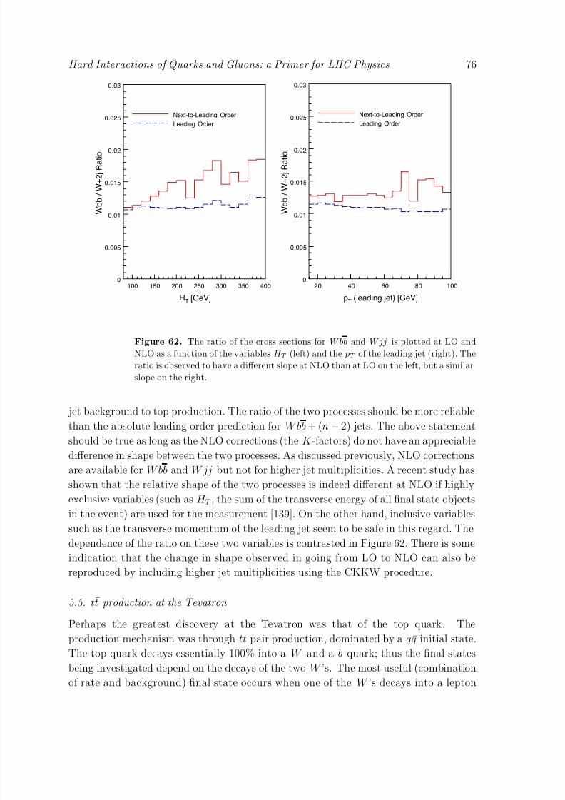
8/3/2019 Hard Interactions of Quarks and Gluons a Primer for LHC Physics
http://slidepdf.com/reader/full/hard-interactions-of-quarks-and-gluons-a-primer-for-lhc-physics 76/118
Hard Interactions of Quarks and Gluons: a Primer for LHC Physics 76
100 150 200 250 300 350 4000
0.005
0.01
0.015
0.02
0.025
0.03
W b b / W + 2 j R a t i o
Next-to-Leading Order
Leading Order
HT [GeV]
20 40 60 80 1000
0.005
0.01
0.015
0.02
0.025
0.03
W b b / W + 2 j R a t i o
Next-to-Leading Order
Leading Order
pT (leading jet) [GeV]
Figure 62. The ratio of the cross sections for W bb and W jj is plotted at LO and
NLO as a function of the variables H T (left) and the pT of the leading jet (right). The
ratio is observed to have a different slope at NLO than at LO on the left, but a similar
slope on the right.
jet background to top production. The ratio of the two processes should be more reliable
than the absolute leading order prediction for W bb + (n − 2) jets. The above statement
should be true as long as the NLO corrections (the K -factors) do not have an appreciable
difference in shape between the two processes. As discussed previously, NLO corrections
are available for W bb and W jj but not for higher jet multiplicities. A recent study has
shown that the relative shape of the two processes is indeed different at NLO if highly
exclusive variables (such as H T , the sum of the transverse energy of all final state objects
in the event) are used for the measurement [139]. On the other hand, inclusive variables
such as the transverse momentum of the leading jet seem to be safe in this regard. The
dependence of the ratio on these two variables is contrasted in Figure 62. There is some
indication that the change in shape observed in going from LO to NLO can also bereproduced by including higher jet multiplicities using the CKKW procedure.
5.5. tt production at the Tevatron
Perhaps the greatest discovery at the Tevatron was that of the top quark. The
production mechanism was through tt pair production, dominated by a qq initial state.
The top quark decays essentially 100% into a W and a b quark; thus the final states
being investigated depend on the decays of the two W ’s. The most useful (combination
of rate and background) final state occurs when one of the W ’s decays into a lepton
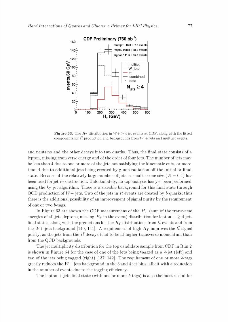
8/3/2019 Hard Interactions of Quarks and Gluons a Primer for LHC Physics
http://slidepdf.com/reader/full/hard-interactions-of-quarks-and-gluons-a-primer-for-lhc-physics 77/118
Hard Interactions of Quarks and Gluons: a Primer for LHC Physics 77
(GeV)TH0 100 200 300 400 500 600
e v e n t s / 6 0 G e V
0
20
40
60
80
100
120
140
160
multijetW+jets
ttcombineddata
35.5 eventssignal: 141.5
2.3 eventsmultijet: 16.0
38.2 eventsWjets: 298.3
)-1
CDF Preliminary (760 pb
4≥jets
N
Figure 63. The H T distribution in W + ≥ 4 jet events at CDF, along with the fitted
components for tt production and backgrounds from W + jets and multijet events.
and neutrino and the other decays into two quarks. Thus, the final state consists of a
lepton, missing transverse energy and of the order of four jets. The number of jets may
be less than 4 due to one or more of the jets not satisfying the kinematic cuts, or more
than 4 due to additional jets being created by gluon radiation off the initial or finalstate. Because of the relatively large number of jets, a smaller cone size (R = 0.4) has
been used for jet reconstruction. Unfortunately, no top analysis has yet been performed
using the kT jet algorithm. There is a sizeable background for this final state through
QCD production of W + jets. Two of the jets in tt events are created by b quarks; thus
there is the additional possibility of an improvement of signal purity by the requirement
of one or two b-tags.
In Figure 63 are shown the CDF measurement of the H T (sum of the transverse
energies of all jets, leptons, missing E T in the event) distribution for lepton + ≥ 4 jets
final states, along with the predictions for the H T distributions from tt events and from
the W + jets background [140, 141]. A requirement of high H T improves the tt signal
purity, as the jets from the tt decays tend to be at higher transverse momentum than
from the QCD backgrounds.
The jet multiplicity distribution for the top candidate sample from CDF in Run 2
is shown in Figure 64 for the case of one of the jets being tagged as a b-jet (left) and
two of the jets being tagged (right) [137, 142]. The requirement of one or more b-tags
greatly reduces the W + jets background in the 3 and 4 jet bins, albeit with a reduction
in the number of events due to the tagging efficiency.
The lepton + jets final state (with one or more b-tags) is also the most useful for

8/3/2019 Hard Interactions of Quarks and Gluons a Primer for LHC Physics
http://slidepdf.com/reader/full/hard-interactions-of-quarks-and-gluons-a-primer-for-lhc-physics 78/118
Hard Interactions of Quarks and Gluons: a Primer for LHC Physics 78
Jet MultiplicityW+1 jet W+2 jet W+3 jet 4 jet≥W+
0
200
400
600
800
1000
1200
Jet MultiplicityW+1 jet W+2 jet W+3 jet 4 jet≥W+
0
200
400
600
800
1000
1200

8/3/2019 Hard Interactions of Quarks and Gluons a Primer for LHC Physics
http://slidepdf.com/reader/full/hard-interactions-of-quarks-and-gluons-a-primer-for-lhc-physics 79/118
Hard Interactions of Quarks and Gluons: a Primer for LHC Physics 79
Figure 66. The PYTHIA predictions for the tt transverse momentum using the
“Plus/Minus” tunes.
larger systematics is that due to the effects of initial state radiation. Jets created by
initial state radiation may replace one or more of the jets from the top quark decays,
affecting the reconstructed top mass. In the past, the initial state radiation (ISR)
systematic was determined by turning the radiation off/on, leading to a relatively large
impact. A more sophisticated treatment was adopted in Run 2, where the tunings
for the parton shower Monte Carlos were modified leading to more/less initial state
radiation, in keeping with the uncertainties associated with Drell-Yan measurements as
discussed in Section 5.1. The resultant tt pair transverse momentum distributions areshown above in Figure 66. The changes to the tt transverse momentum distribution
created by the tunes are relatively modest, as is the resultant systematic error on the
top mass determination.
Note that the peak of the tt transverse momentum spectrum is slightly larger than
that for Z production at the Tevatron, due to the larger mass of the tt system. As both
are produced primarily by qq initial states, the differences are not large.
It is also interesting to look at the mass distribution of the tt system, as new physics
(such as a Z ′ [144]) might couple preferentially to top quarks. Such a comparison for
CDF Run 2 is shown in Figure 67 where no signs of a high mass resonance are evident.
If we look at predictions for the tt mass distribution at NLO, we see that the NLO cross
section is substantially less than the LO one at high mass (see Figure 68). This should
be taken into account in any searches for new physics at high tt mass.
Further investigation shows that the decrease of NLO compared to LO at high
mass is found only in the qq initial state and not in the gg initial state. In fact, at
the Tevatron, the ratio of NLO to LO for gg initial states grows dramatically with
increasing top pair invariant mass. This effect is largely due to the increase in the gluon
distribution when going from CTEQ6L1 in the LO calculation to CTEQ6M at NLO.
For instance, at x ∼ 0.4 (and hence an invariant mass of about 800 GeV) the gluon

8/3/2019 Hard Interactions of Quarks and Gluons a Primer for LHC Physics
http://slidepdf.com/reader/full/hard-interactions-of-quarks-and-gluons-a-primer-for-lhc-physics 80/118
Hard Interactions of Quarks and Gluons: a Primer for LHC Physics 80
Figure 67. The tt mass distribution as observed by CDF in Run 2.
Figure 68. The ratio of the NLO to LO predictions for the tt mass at the Tevatron.
The predictions include the ratio for the total cross section and for the specific qq and
gg initial states. Note that the total also includes a gq contribution (not present atLO) and that the gg ratio is divided by a factor of 3.
distribution is about a factor two larger in CTEQ6M than in CTEQ6L1, giving a factor
four increase in the cross section. Conversely, the quark distribution is slightly decreased
at such large x. However, the absolute contribution of the tt cross at high masses from
gg initial states is small, due to the rapidly falling gluon distribution at high x.

8/3/2019 Hard Interactions of Quarks and Gluons a Primer for LHC Physics
http://slidepdf.com/reader/full/hard-interactions-of-quarks-and-gluons-a-primer-for-lhc-physics 81/118
Hard Interactions of Quarks and Gluons: a Primer for LHC Physics 81
6. Benchmarks for the LHC
6.1. Introduction
Scattering at the LHC is not simply rescaled scattering at the Tevatron. For many of thekey processes the typical momentum fractions x are small; thus, there is a dominance of
sea quark and gluon scattering as compared to valence quark scattering at the Tevatron.
There is a large phase space for gluon emission and thus intensive QCD backgrounds
for many of the signatures of new physics. Many of the scales relating to interesting
processes are large compared to the W mass; thus, electroweak corrections can become
important even for nominally QCD processes. In this section, we will try to provide
some useful benchmarks for LHC predictions.
6.2. Parton-parton luminosities at the LHC
‡It is useful to return to the idea of differential parton-parton luminosities. Such
luminosities, when multiplied by the dimensionless cross section sσ for a given process,
provide a useful estimate of the size of an event cross section at the LHC. Below we
define the differential parton-parton luminosity dLij/ds dy and its integral dLij/ds:
dLij
ds dy=
1
s
1
1 + δij[f i(x1, µ)f j(x2, µ) + (1 ↔ 2)] . (46)
The prefactor with the Kronecker delta avoids double-counting in case the partons are
identical. The generic parton-model formula
σ =i,j
10 dx1 dx2 f i(x1, µ) f j(x2, µ) σij (47)
can then be written as
σ =i,j
ds
sdy
dLij
ds dy
(s σij) . (48)
(Note that this result is easily derived by defining τ = x1 x2 = s/s and observing that
the Jacobian ∂ (τ, y)/∂ (x1, x2) = 1.)
Equation (48) can be used to estimate the production rate for a hard scattering
process at the LHC as follows. Figure 69 shows a plot of the luminosity function
integrated over rapidity, dLij/ds =
(dLij/ds dy) dy, at the LHC √s = 14TeV forvarious parton flavour combinations, calculated using the CTEQ6.1 parton distribution
functions [11]. The widths of the curves indicate an estimate for the pdf uncertainties.
We assume µ =√
s for the scale §. As expected, the gg luminosity is large at low√
s
but falls rapidly with respect to the other parton luminosities. The gq luminosity is
large over the entire kinematic region plotted.
‡ Parts of this discussion also appeared in a contribution to the Les Houches 2005 proceedings [149]
by A. Belyaev, J. Huston and J. Pumplin§ Similar plots made with earlier pdfs are shown in Ellis, Stirling, Webber [8]

8/3/2019 Hard Interactions of Quarks and Gluons a Primer for LHC Physics
http://slidepdf.com/reader/full/hard-interactions-of-quarks-and-gluons-a-primer-for-lhc-physics 82/118
Hard Interactions of Quarks and Gluons: a Primer for LHC Physics 82
Figure 69. The parton-parton luminositydLij
dτ
in picobarns, integrated over y.
Green=gg, Blue=
i(gqi + gqi + qig + qig), Red=
i(qiqi + qiqi), where the sum runs
over the five quark flavours d, u, s, c, b.
Figures 70 and 71 present the second product, [sσij ], for various 2 → 2 partonic
processes with massless and massive partons in the final state respectively. The parton
level cross sections have been calculated for a parton pT > 0.1 ×√
s cut and for fixedαS = 0.118 using the CalcHEP package [150]. For the case of massive partons in the
final state, there is a threshold behaviour not present with massless partons. Note also
that the threshold behaviour is different for qq and gg initial states. The gg processes
can proceed through the t-channel as well as the s-channel and this is responsible for
the extra structure.
The products [sσij ] are plotted for massless and massive final state partons as a
function of the ratio pT /√
s in Figures 72 and 73. One can use (48) in the form
σ =∆s
s
dLij
ds
(s σij) . (49)
and Figures 70, 72, 71, 73 to estimate the QCD production cross sections for a given ∆ s
interval and a particular cut on pT /√
s. For example, for the gg → gg rate for s=1 TeV
and ∆s = 0.01s, we have dLgg/ds ≃ 103 pb and s σgg ≃ 20 leading to σ ≃ 200 pb (for
the pgT > 0.1 × √
s cut we have used above). Note that for a given small ∆ s/s interval,
the corresponding invariant mass ∆√
s/√
s interval, is ∆√
s/√
s ≃ 12
∆s/s. One should
also mention that all hard cross sections presented in Figure 70 are proportional to α2S
and have been calculated for αS = 0.118, so production rates can be easily rescaled for
a particular αS at a given scale.

8/3/2019 Hard Interactions of Quarks and Gluons a Primer for LHC Physics
http://slidepdf.com/reader/full/hard-interactions-of-quarks-and-gluons-a-primer-for-lhc-physics 83/118
Hard Interactions of Quarks and Gluons: a Primer for LHC Physics 83
gg → gg
gg → qq –
gq → gq
qq → qq qq´ → qq´, qq – ´ → qq
– ´
qq – → q´q
– ´
qq – → qq
–
qq – → gg
√S ^(TeV)
σ ^ x
S ^
10 -3
10 -2
10 -1
1
10
0 2 4 6 8 10
Figure 70. Parton level cross sections (sσij) for various processes involving massless
partons in the final state.
gg → tt –
qq – → tt
–
gg → bb –
qq – → bb
–
qq – → W
+ W
-
√S ^(TeV)
σ ^ x
S ^
10 -3
10 -2
0 2 4 6 8 10
Figure 71. Parton level cross sections (sσij) for various processes involving massive
partons in the final state.
One can further specify the parton-parton luminosity for a specific rapidity y and
s, dLij/ds dy. If one is interested in a specific partonic initial state, then the resulting
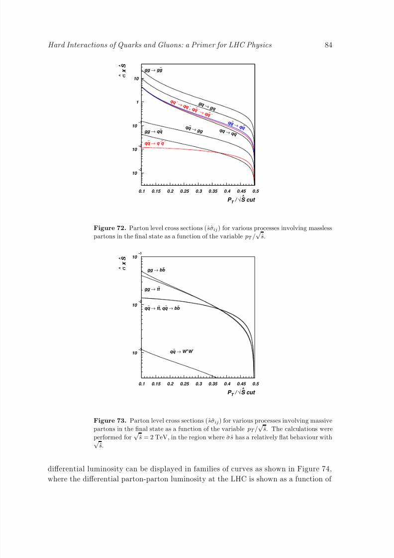
8/3/2019 Hard Interactions of Quarks and Gluons a Primer for LHC Physics
http://slidepdf.com/reader/full/hard-interactions-of-quarks-and-gluons-a-primer-for-lhc-physics 84/118
Hard Interactions of Quarks and Gluons: a Primer for LHC Physics 84
gg → gg –
qq – → q´q
– ´
gg → qq –
g q → g q
q q → q q , q q – ´ → q q
– ´
q q –
→ g g
q q – → q q
–
q q → q q
P T / √S ^
cut
σ ^ x
S ^
10 -3
10 -2
10 -1
1
10
0.1 0.15 0.2 0.25 0.3 0.35 0.4 0.45 0.5
Figure 72. Parton level cross sections (sσij) for various processes involving massless
partons in the final state as a function of the variable pT /√
s.
gg → tt –
qq – → tt
– → bb
–
gg → bb –
qq – → W
+ W
-
P T / √S ^
cut
σ ^ x
S ^
10 -3
10 -2
10 -1
0.1 0.15 0.2 0.25 0.3 0.35 0.4 0.45 0.5
Figure 73. Parton level cross sections (sσij) for various processes involving massive
partons in the final state as a function of the variable pT /√
s. The calculations were
performed for√
s = 2 TeV, in the region where σs has a relatively flat behaviour with√s.
differential luminosity can be displayed in families of curves as shown in Figure 74,
where the differential parton-parton luminosity at the LHC is shown as a function of

8/3/2019 Hard Interactions of Quarks and Gluons a Primer for LHC Physics
http://slidepdf.com/reader/full/hard-interactions-of-quarks-and-gluons-a-primer-for-lhc-physics 85/118
Hard Interactions of Quarks and Gluons: a Primer for LHC Physics 85
Figure 74. d(Luminosity)/dy at rapidities (right to left) y = 0, 2, 4, 6. Green=gg,
Blue=
i(gqi + gqi + qig + qig), Red=
i(qiqi + qiqi), where the sum runs over the five
quark flavours d, u, s, c, b.
the subprocess centre-of-mass energy√
s at various values of rapidity for the produced
system for several different combinations of initial state partons. One can read from the
curves the parton-parton luminosity for a specific value of mass fraction and rapidity.
(It is also easy to use the Durham pdf plotter to generate the pdf curve for any desired
flavour and kinematic configuration .)It is also of great interest to understand the uncertainty in the parton-parton
luminosity for specific kinematic configurations. Some representative parton-parton
luminosity uncertainties, integrated over rapidity, are shown in Figures 75, 76 and 77.
The pdf uncertainties were generated from the CTEQ6.1 Hessian error analysis using the
standard ∆χ2 = 100 criterion. Except for kinematic regions where one or both partons
is a gluon at high x, the pdf uncertainties are of the order of 5–10%. Luminosity
uncertainties for specific rapidity values are available at the SM benchmark website.
Even tighter constraints will be possible once the LHC Standard Model data is included
in the global pdf fits. Again, the uncertainties for individual pdfs can also be calculated
online using the Durham pdf plotter. Often it is not the pdf uncertainty for a cross
section that is required, but rather the pdf uncertainty for an acceptance for a given final
state. The acceptance for a particular process may depend on the input pdfs due to the
rapidity cuts placed on the jets, leptons, photons, etc. and the impacts of the varying
longitudinal boosts of the final state caused by the different pdf pairs. An approximate
“rule-of-thumb” is that the pdf uncertainty for the acceptance is a factor of 5–10 times
smaller than the uncertainty for the cross section itself.
http://durpdg.dur.ac.uk/hepdata/pdf3.html

8/3/2019 Hard Interactions of Quarks and Gluons a Primer for LHC Physics
http://slidepdf.com/reader/full/hard-interactions-of-quarks-and-gluons-a-primer-for-lhc-physics 86/118
Hard Interactions of Quarks and Gluons: a Primer for LHC Physics 86
Figure 75. Fractional uncertainty of the gg luminosity integrated over y.
Figure 76. Fractional uncertainty for the parton-parton luminosity integrated over y
for
i(qiqi + qiqi), where the sum runs over the five quark flavours d, u, s, c, b.
In Figure 78, the pdf luminosity curves shown in Figure 69 are overlaid with
equivalent luminosity curves from the Tevatron. In Figure 79, the ratios of the pdf
luminosities at the LHC to those at the Tevatron are plotted. The most dramatic

8/3/2019 Hard Interactions of Quarks and Gluons a Primer for LHC Physics
http://slidepdf.com/reader/full/hard-interactions-of-quarks-and-gluons-a-primer-for-lhc-physics 87/118
Hard Interactions of Quarks and Gluons: a Primer for LHC Physics 87
Figure 77. Fractional uncertainty for the luminosity integrated over y for
i(qiqi +
qiqi), where the sum runs over the five quark flavours d, u, s, c, b.
Figure 78. The parton-parton luminosity1s
dLij
dτ
in pb integrated over y. Green=gg,
Blue=
i(gqi + gqi + qig + qig), Red=
i(qiqi + qiqi), where the sum runs over the five
quark flavours d, u, s, c, b. The top family of curves are for the LHC and the bottom
for the Tevatron.
increase in pdf luminosity at the LHC comes from gg initial states, followed by gq
initial states and then qq initial states. The latter ratio is smallest because of the
availability of valence antiquarks at the Tevatron at moderate to large x. As an example,

8/3/2019 Hard Interactions of Quarks and Gluons a Primer for LHC Physics
http://slidepdf.com/reader/full/hard-interactions-of-quarks-and-gluons-a-primer-for-lhc-physics 88/118
Hard Interactions of Quarks and Gluons: a Primer for LHC Physics 88
Figure 79. The ratio of parton-parton luminosity1s
dLij
dτ
in pb integrated over y at
the LHC and Tevatron. Green=gg (top), Blue=
i(gqi + gqi + qig + qig) (middle),
Red=
i(qiqi + qiqi) (bottom), where the sum runs over the five quark flavours d, u,
s, c, b.
consider chargino pair production with√
s = 0.4 TeV. This process proceeds through
qq annihilation; thus, there is only a factor of 10 enhancement at the LHC compared to
the Tevatron.
Backgrounds to interesting physics at the LHC proceed mostly through gg and gqinitial states. Thus, there will be a commensurate increase in the rate for background
processes at the LHC.
6.3. Stability of NLO global analyses
The W and Z cross sections at the LHC are shown in Figure 80. The MRST2004
predictions are shown at LO, NLO and NNLO; also shown are the CTEQ6.1 predictions
at NLO, along with the CTEQ6.1 pdf error band. There is a significant increase in cross
section when going from LO to NLO, and then a small decrease when going from NLO
to NNLO. The NLO MRST2004 and CTEQ6.1 predicted cross sections agree with eachother, well within the CTEQ6.1 pdf uncertainty band.
Most of the absolute predictions for LHC observables have been carried out at NLO,
i.e. with NLO pdfs and with NLO matrix elements. Such predictions have worked well
at the Tevatron, but the LHC explores a new region of (small) x for a hadron-hadron
collider. Thus, it is important to understand whether the NLO formalism carries over to
the LHC with the same degree of accuracy. In recent years, some preliminary next-to-
next-leading-order global pdf analyses have been carried out either for DIS alone [151],
or in a global analysis context [153]. The differences with respect to the corresponding
NLO analyses are reasonably small. However, most observables of interest (including
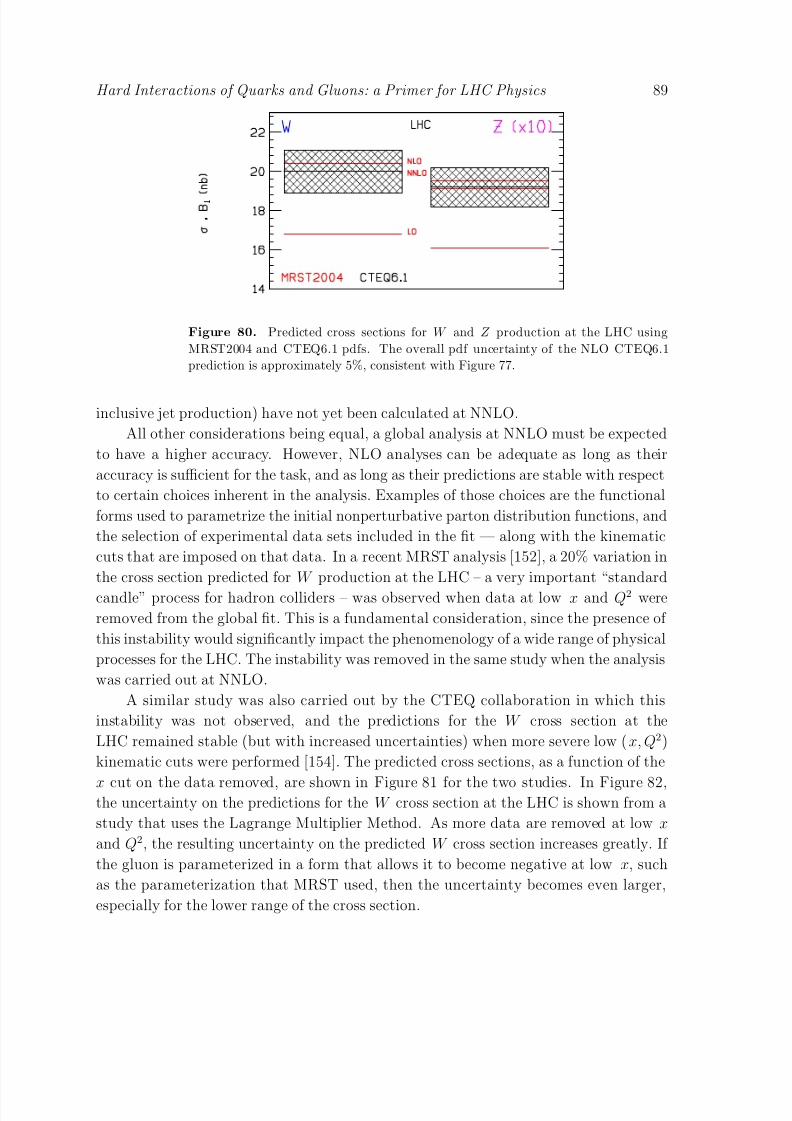
8/3/2019 Hard Interactions of Quarks and Gluons a Primer for LHC Physics
http://slidepdf.com/reader/full/hard-interactions-of-quarks-and-gluons-a-primer-for-lhc-physics 89/118
Hard Interactions of Quarks and Gluons: a Primer for LHC Physics 89
Figure 80. Predicted cross sections for W and Z production at the LHC using
MRST2004 and CTEQ6.1 pdfs. The overall pdf uncertainty of the NLO CTEQ6.1
prediction is approximately 5%, consistent with Figure 77.
inclusive jet production) have not yet been calculated at NNLO.
All other considerations being equal, a global analysis at NNLO must be expected
to have a higher accuracy. However, NLO analyses can be adequate as long as their
accuracy is sufficient for the task, and as long as their predictions are stable with respect
to certain choices inherent in the analysis. Examples of those choices are the functional
forms used to parametrize the initial nonperturbative parton distribution functions, and
the selection of experimental data sets included in the fit — along with the kinematic
cuts that are imposed on that data. In a recent MRST analysis [152], a 20% variation in
the cross section predicted for W production at the LHC – a very important “standard
candle” process for hadron colliders – was observed when data at low x and Q2 were
removed from the global fit. This is a fundamental consideration, since the presence of
this instability would significantly impact the phenomenology of a wide range of physical
processes for the LHC. The instability was removed in the same study when the analysis
was carried out at NNLO.
A similar study was also carried out by the CTEQ collaboration in which this
instability was not observed, and the predictions for the W cross section at the
LHC remained stable (but with increased uncertainties) when more severe low (x, Q2)
kinematic cuts were performed [154]. The predicted cross sections, as a function of the
x cut on the data removed, are shown in Figure 81 for the two studies. In Figure 82,the uncertainty on the predictions for the W cross section at the LHC is shown from a
study that uses the Lagrange Multiplier Method. As more data are removed at low x
and Q2, the resulting uncertainty on the predicted W cross section increases greatly. If
the gluon is parameterized in a form that allows it to become negative at low x, such
as the parameterization that MRST used, then the uncertainty becomes even larger,
especially for the lower range of the cross section.

8/3/2019 Hard Interactions of Quarks and Gluons a Primer for LHC Physics
http://slidepdf.com/reader/full/hard-interactions-of-quarks-and-gluons-a-primer-for-lhc-physics 90/118
Hard Interactions of Quarks and Gluons: a Primer for LHC Physics 90
Figure 81. Predicted total cross section of W + + W − production at the LHC for the
fits obtained in the CTEQ stability study, compared to the MRST results. The overallpdf uncertainty of the prediction is ∼ 5%, as observed in Figure 77.
Figure 82. Lagrange multiplier results for the W cross section (in nb) at the LHC
using a positive-definite gluon. The three curves, in order of decreasing steepness,
correspond to three sets of kinematic cuts, standard/intermediate/strong.
6.4. The future for NLO calculations
Unfortunately, our ability to take advantage of the benefits of NLO predictions is severely
limited by the calculations available. Currently, no complete NLO QCD calculation
exists for a process involving more than 5 particles. This means that we are limited
to the consideration of scenarios such as 4 jet production at LEP (effectively a 1 → 4
process) and a number of 2 → 3 processes of interest at hadron colliders.

8/3/2019 Hard Interactions of Quarks and Gluons a Primer for LHC Physics
http://slidepdf.com/reader/full/hard-interactions-of-quarks-and-gluons-a-primer-for-lhc-physics 91/118
Hard Interactions of Quarks and Gluons: a Primer for LHC Physics 91
The bottleneck for these calculations is the evaluation of the loop diagrams. The
real radiation component consists of the evaluation of known lowest order matrix
elements combined with a method for systematically removing their singularities, several
of which are well understood. In contrast, the evaluation of the virtual contribution must
at present be performed on a case-by-case basis. Even the most basic integral that can
appear depends non-trivially on the number of external legs in the loop, as well as on
the masses of all the external and internal particles. To complicate matters further,
the presence of powers of loop momenta in the integrals (from fermion propagators or
multi-gluon vertices) leads to “tensor integrals” which typically are expressed as the
sum of many terms. Taken all together, this means that traditional methods based on
an analytical Feynman diagram approach are already limited by the computing power
currently available. It seems unlikely that further progress, such as the NLO calculation
of a 2 → 4 process, will be made in this fashion.
An alternative to this brute-force Feynman diagram approach is provided by“unitarity-based” methods, which are based on sewing together tree level amplitudes
(for a review, see [155]). These methods rely on the Cutkosky rules to generate the
1-loop amplitude by summing over all possible cuts of sewn-together tree amplitudes.
Although this knowledge in itself only suffices for sufficiently supersymmetric theories,
results for 1-loop amplitudes in non-supersymmetric theories (such as QCD) can be
obtained by consideration of collinear limits of the amplitudes. Such techniques were
used to obtain relatively compact expressions for the 1-loop amplitudes required to
evaluate the process e+e− → 4 partons [52].
More recently the “twistor-inspired” methods, which have proven so efficient at
generating compact expressions for tree-level amplitudes, have been considered atthe 1-loop level [156]. The MHV rules (discussed in Section 3.2.3) were shown to
reproduce known results at the 1-loop level [157] and their application has passed
from calculations in N = 4 supersymmetric Yang-Mills theory to the evaluation of
amplitudes in QCD ([158] and references therein). Similarly, the on-shell recursion
relations have proven equally useful at one-loop [159], even allowing for the calculation
of MHV amplitudes involving an arbitrary number of gluons [160]. These methods will
doubtless be refined and extended to more complicated calculations over time.
An alternative path to 1-loop amplitudes is provided by numerical approaches. Such
techniques have long been applied at lowest order, with the main attraction derivingfrom the promise of a generic solution that can be applied to any process (given sufficient
computing power). The techniques are generally either completely numerical evaluations
of loop integrals [161, 162], or they are semi-numerical approaches that perform only the
tensor integral reductions numerically [163, 164, 165, 166, 167, 168]. In most cases these
algorithms have only been applied to individual integrals or diagrams, although one
recent application evaluates the 1-loop matrix elements for the Higgs+4 parton process
(which is otherwise uncalculated) [169] ¶. Once more, the study of these approaches is
¶ All partons are treated as outgoing so this process corresponds to a Higgs+2 parton final state
8/3/2019 Hard Interactions of Quarks and Gluons a Primer for LHC Physics
http://slidepdf.com/reader/full/hard-interactions-of-quarks-and-gluons-a-primer-for-lhc-physics 92/118
Hard Interactions of Quarks and Gluons: a Primer for LHC Physics 92
in its infancy and the coming years promise significant further development.
It should also be noted that many of the recent simplifying techniques and
numerical approaches have concentrated on processes involving gluons and massless
quarks. Although this is sufficient for many hadron collider applications, there are
many processes for which a calculation which includes the quark mass is necessary. The
top quark mass must clearly be taken into account and, in addition, the experimental
ability to identify b-quarks in events often demands that the mass of the bottom quark is
included. When including the mass, the evaluation of Feynman diagrams becomes much
more complicated and the expressions for amplitudes do not simplify as conveniently.
However, the presence of an additional hard scale renders the loop amplitudes less
infrared divergent, so that some numerical approaches may in fact benefit from the
inclusion of quark masses. Due to the large role of the top quark in much of the LHC
program, advances on this front are to be expected in the near future.
6.5. A realistic NLO wishlist for multi-parton final states at the LHC
A somewhat whimsical experimenter’s wishlist was first presented at the Run 2 Monte
Carlo workshop at Fermilab in 2001 †. Since then the list has gathered a great deal
of notoriety and has appeared in numerous LHC-related theory talks. It is unlikely
that W W W + bb + 3 jets will be calculated at NLO soon, no matter the level of
physics motivation, but there are a number of high priority calculations, primarily of
backgrounds to new physics, that are accessible with the present technology. However,
the manpower available before the LHC turns on is limited. Thus, it is necessary to
prioritize the calculations, both in terms of the importance of the calculation and theeffort expected to bring it to completion.
A prioritized list, determined at the Les Houches 2005 Workshop, is shown in
Table 2, along with a brief discussion of the physics motivation. Note that the list
contains only 2 → 3 and 2 → 4 processes, as these are feasible to be completed by the
turn on of the LHC.
First, a few general statements: in general, signatures for new physics will involve
high pT leptons and jets (especially b jets) and missing transverse momentum. Thus,
backgrounds to new physics will tend to involve (multiple) vector boson production
(with jets) and tt pair production (with jets). The best manner in which to understand
the normalization of a cross section is to measure it; however the rates for some of thecomplex final states listed here may be limited and (at least in the early days) must
be calculated from NLO theory. As discussed at length previously, NLO is the first
order at which both the normalization and shape can be calculated with any degree of
confidence.
We now turn to a detailed look at each of these processes:
• pp → V V + jet: One of the most promising channels for Higgs boson production
in the low mass range is through the H → W W ∗ channel, with the W ’s decaying
†http://vmsstreamer1.fnal.gov/Lectures/MonteCarlo2001/Index.htm

8/3/2019 Hard Interactions of Quarks and Gluons a Primer for LHC Physics
http://slidepdf.com/reader/full/hard-interactions-of-quarks-and-gluons-a-primer-for-lhc-physics 93/118
Hard Interactions of Quarks and Gluons: a Primer for LHC Physics 93
process relevant for
(V ∈ {Z,W,γ })
1. pp → V V +jet ttH , new physics
2. pp → H + 2 jets H production by vector boson fusion (VBF)
3. pp → tt bb ttH
4. pp → tt + 2 jets ttH
5. pp → V V bb VBF→ H → V V , ttH , new physics
6. pp → V V + 2 jets VBF→ H → V V
7. pp → V + 3 jets various new physics signatures
8. pp → V V V SUSY trilepton searches
Table 2. The wishlist of processes for which a NLO calculation is both desired and
feasible in the near future.
semi-leptonically. It is useful to look both in the H → W W exclusive channel,
along with the H → W W +jet channel. The calculation of pp → W W +jet will be
especially important in understanding the background to the latter.
• pp → H + 2 jets: A measurement of vector boson fusion (VBF) production of the
Higgs boson will allow the determination of the Higgs coupling to vector bosons.
One of the key signatures for this process is the presence of forward-backward
tagging jets. Thus, QCD production of H + 2 jets must be understood, especially
as the rates for the two are comparable in the kinematic regions of interest.
• pp → ttbb and pp → tt + 2 jets: Both of these processes serve as background to
ttH , where the Higgs boson decays into a bb pair. The rate for ttjj is much greater
than that for ttbb and thus, even if 3 b-tags are required, there may be a significant
chance for the heavy flavour mistag of a ttjj event to contribute to the background.
• pp → V V bb: Such a signature serves as non-resonant background to tt production
as well as to possible new physics.
•pp
→V V + 2 jets: The process serves as a background to VBF production of a
Higgs boson.
• pp → V + 3 jets: The process serves as background for tt production where one
of the jets may not be reconstructed, as well as for various new physics signatures
involving leptons, jets and missing transverse momentum.
• pp → V V V : The process serves as a background for various new physics
subprocesses such as SUSY tri-lepton production.
Work on (at least) the processes 1. to 4. of Table 2 is already in progress by several
groups, and clearly all of them aim at a setup which allows for a straightforward
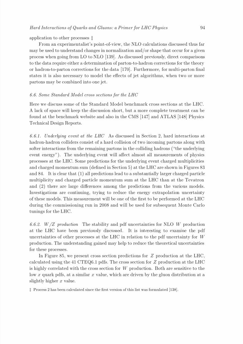
8/3/2019 Hard Interactions of Quarks and Gluons a Primer for LHC Physics
http://slidepdf.com/reader/full/hard-interactions-of-quarks-and-gluons-a-primer-for-lhc-physics 94/118
Hard Interactions of Quarks and Gluons: a Primer for LHC Physics 94
application to other processes ‡From an experimentalist’s point-of-view, the NLO calculations discussed thus far
may be used to understand changes in normalization and/or shape that occur for a given
process when going from LO to NLO [139]. As discussed previously, direct comparisons
to the data require either a determination of parton-to-hadron corrections for the theory
or hadron-to-parton corrections for the data [170]. Furthermore, for multi-parton final
states it is also necessary to model the effects of jet algorithms, when two or more
partons may be combined into one jet.
6.6. Some Standard Model cross sections for the LHC
Here we discuss some of the Standard Model benchmark cross sections at the LHC.
A lack of space will keep the discussion short, but a more complete treatment can be
found at the benchmark website and also in the CMS [147] and ATLAS [148] Physics
Technical Design Reports.
6.6.1. Underlying event at the LHC As discussed in Section 2, hard interactions at
hadron-hadron colliders consist of a hard collision of two incoming partons along with
softer interactions from the remaining partons in the colliding hadrons (“the underlying
event energy”). The underlying event will affect almost all measurements of physics
processes at the LHC. Some predictions for the underlying event charged multiplicities
and charged momentum sum (defined in Section 5) at the LHC are shown in Figures 83
and 84. It is clear that (1) all predictions lead to a substantially larger charged particle
multiplicity and charged particle momentum sum at the LHC than at the Tevatronand (2) there are large differences among the predictions from the various models.
Investigations are continuing, trying to reduce the energy extrapolation uncertainty
of these models. This measurement will be one of the first to be performed at the LHC
during the commissioning run in 2008 and will be used for subsequent Monte Carlo
tunings for the LHC.
6.6.2. W / Z production The stability and pdf uncertainties for NLO W production
at the LHC have been previously discussed. It is interesting to examine the pdf
uncertainties of other processes at the LHC in relation to the pdf uncertainty for W
production. The understanding gained may help to reduce the theoretical uncertainties
for these processes.
In Figure 85, we present cross section predictions for Z production at the LHC,
calculated using the 41 CTEQ6.1 pdfs. The cross section for Z production at the LHC
is highly correlated with the cross section for W production. Both are sensitive to the
low x quark pdfs, at a similar x value, which are driven by the gluon distribution at a
slightly higher x value.
‡ Process 2 has been calculated since the first version of this list was formulated [138].
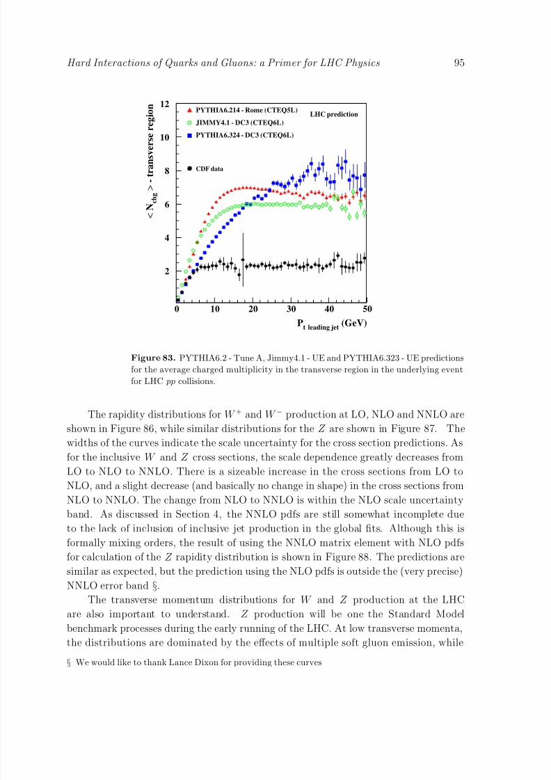
8/3/2019 Hard Interactions of Quarks and Gluons a Primer for LHC Physics
http://slidepdf.com/reader/full/hard-interactions-of-quarks-and-gluons-a-primer-for-lhc-physics 95/118
Hard Interactions of Quarks and Gluons: a Primer for LHC Physics 95
2
4
6
8
10
12
0 10 20 30 40 50
CDF data
PYTHIA6.214 - Rome (CTEQ5L)
JIMMY4.1 - DC3 (CTEQ6L)
PYTHIA6.324 - DC3 (CTEQ6L)
LHC prediction
Pt leading jet
(GeV)
<
N c h g
>
- t r a n s v e r s e
r e g i o n
Figure 83. PYTHIA6.2 - Tune A, Jimmy4.1 - UE and PYTHIA6.323 - UE predictions
for the average charged multiplicity in the transverse region in the underlying event
for LHC pp collisions.
The rapidity distributions for W + and W − production at LO, NLO and NNLO are
shown in Figure 86, while similar distributions for the Z are shown in Figure 87. The
widths of the curves indicate the scale uncertainty for the cross section predictions. As
for the inclusive W and Z cross sections, the scale dependence greatly decreases from
LO to NLO to NNLO. There is a sizeable increase in the cross sections from LO to
NLO, and a slight decrease (and basically no change in shape) in the cross sections from
NLO to NNLO. The change from NLO to NNLO is within the NLO scale uncertainty
band. As discussed in Section 4, the NNLO pdfs are still somewhat incomplete due
to the lack of inclusion of inclusive jet production in the global fits. Although this is
formally mixing orders, the result of using the NNLO matrix element with NLO pdfsfor calculation of the Z rapidity distribution is shown in Figure 88. The predictions are
similar as expected, but the prediction using the NLO pdfs is outside the (very precise)
NNLO error band §.
The transverse momentum distributions for W and Z production at the LHC
are also important to understand. Z production will be one the Standard Model
benchmark processes during the early running of the LHC. At low transverse momenta,
the distributions are dominated by the effects of multiple soft gluon emission, while
§ We would like to thank Lance Dixon for providing these curves
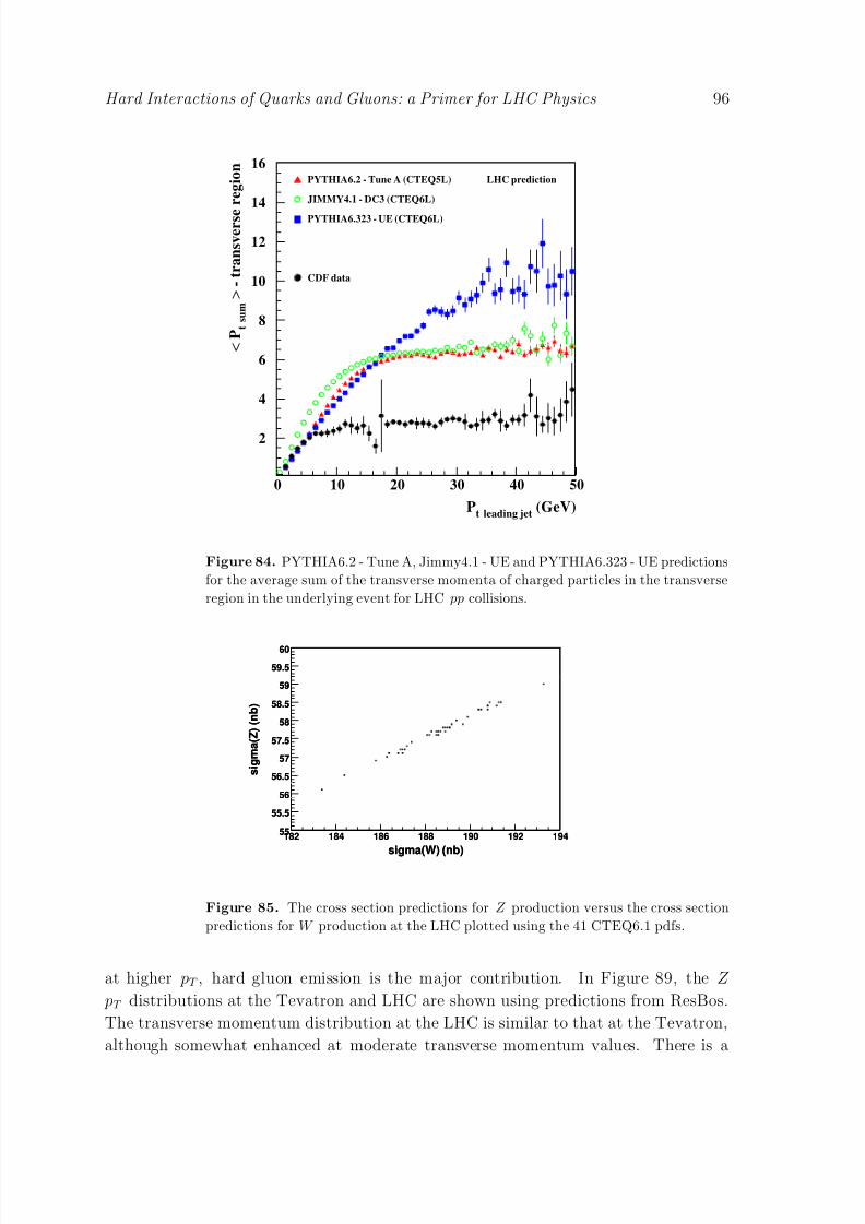
8/3/2019 Hard Interactions of Quarks and Gluons a Primer for LHC Physics
http://slidepdf.com/reader/full/hard-interactions-of-quarks-and-gluons-a-primer-for-lhc-physics 96/118
Hard Interactions of Quarks and Gluons: a Primer for LHC Physics 96
2
4
6
8
10
12
14
16
0 10 20 30 40 50
CDF data
PYTHIA6.2 - Tune A (CTEQ5L)
JIMMY4.1 - DC3 (CTEQ6L)
PYTHIA6.323 - UE (CTEQ6L)
LHC prediction
Pt leading jet
(GeV)
<
P t s u m >
- t r a n s v e r s e
r e g i o n
Figure 84. PYTHIA6.2 - Tune A, Jimmy4.1 - UE and PYTHIA6.323 - UE predictions
for the average sum of the transverse momenta of charged particles in the transverse
region in the underlying event for LHC pp collisions.
sigma(W) (nb)
182 184 186 188 190 192 194
s i g m a ( Z ) ( n b )
55
55.5
56
56.5
57
57.5
58
58.5
59
59.5
60
ScaleT
Jet20 corrected Mulitple Interactions and Hadron P
sigma(W) (nb)
182 184 186 188 190 192 194
s i g m a ( Z ) ( n b )
55
55.5
56
56.5
57
57.5
58
58.5
59
59.5
60
Figure 85. The cross section predictions for Z production versus the cross section
predictions for W production at the LHC plotted using the 41 CTEQ6.1 pdfs.
at higher pT , hard gluon emission is the major contribution. In Figure 89, the Z
pT distributions at the Tevatron and LHC are shown using predictions from ResBos.
The transverse momentum distribution at the LHC is similar to that at the Tevatron,
although somewhat enhanced at moderate transverse momentum values. There is a

8/3/2019 Hard Interactions of Quarks and Gluons a Primer for LHC Physics
http://slidepdf.com/reader/full/hard-interactions-of-quarks-and-gluons-a-primer-for-lhc-physics 97/118
Hard Interactions of Quarks and Gluons: a Primer for LHC Physics 97
Figure 86. The rapidity distributions for W + and W − production at the LHC at
LO, NLO and NNLO.
Figure 87. The rapidity distributions for Z production at the LHC at LO, NLO and
NNLO.
larger phase space for gluon emission of incident quarks at x = 0.007 (Z production
at the LHC) than for incident quarks at x = 0.05 (Z production at the Tevatron)
and the enhancement at moderate transverse momentum is a result of this. There is
still substantial influence of the non-perturbative component of the parton transverse
momentum near the peak region of the Z transverse momentum distribution [171].
An analysis of semi-inclusive deep-inelastic scattering hadroproduction suggests a
broadening of transverse momentum distributions for x values below 10−3 to 10−2 [173].
(See also the discussion in Section 6.6.3.) The pT broadening at small x may be
due to x-dependent higher order contributions (like BFKL [174, 175, 176, 177]) not
included in current resummation formalisms. Such contributions are important when
log Q2 ≪ log(1/x). The BFKL formalism resums terms proportional to αS log(1/x),
retaining the full Q2 dependence. The BFKL corrections would have a small impact
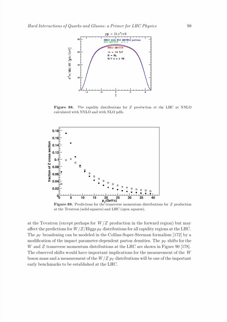
8/3/2019 Hard Interactions of Quarks and Gluons a Primer for LHC Physics
http://slidepdf.com/reader/full/hard-interactions-of-quarks-and-gluons-a-primer-for-lhc-physics 98/118
Hard Interactions of Quarks and Gluons: a Primer for LHC Physics 98
Figure 88. The rapidity distributions for Z production at the LHC at NNLO
calculated with NNLO and with NLO pdfs.
(GeV/c)T
p0 5 10 15 20 25 30 35 40
f r a c t i o n o f Z c r o s s s e c t i o n
0
0.02
0.04
0.06
0.08
0.1
0.12
0.14
0.16
0.18
Figure 89. Predictions for the transverse momentum distributions for Z production
at the Tevatron (solid squares) and LHC (open squares).
at the Tevatron (except perhaps for W /Z production in the forward region) but may
affect the predictions for W /Z /Higgs pT distributions for all rapidity regions at the LHC.
The pT broadening can be modeled in the Collins-Soper-Sterman formalism [172] by a
modification of the impact parameter-dependent parton densities. The pT shifts for the
W and Z transverse momentum distributions at the LHC are shown in Figure 90 [178].
The observed shifts would have important implications for the measurement of the W
boson mass and a measurement of the W /Z pT distributions will be one of the important
early benchmarks to be established at the LHC.

8/3/2019 Hard Interactions of Quarks and Gluons a Primer for LHC Physics
http://slidepdf.com/reader/full/hard-interactions-of-quarks-and-gluons-a-primer-for-lhc-physics 99/118
Hard Interactions of Quarks and Gluons: a Primer for LHC Physics 99
W, Z Production at LHC
0
0.05
0.10
0.15
0.20
0.25
2.5 5 7.5 10 12.5 15 17.5 20 22.5
ρ(x) = 0
ρ(x) ≠ 0, c0
= 0.013, x0
= 0.005
pp → W+
X → e+ ν X
| ye
| < 2.5
pTe
, E/ T ν > 25 GeV
0
0.5
1
1.5
2
2.5
3
0 2.5 5 7.5 10 12.5 15 17.5 20 22.5 25
qT
[GeV]
d σ / d q T
[ n b / G e V ]
pp → Z0
X
Figure 90. The predictions for the transverse momentum distributions for W and Z
production with and without the pT -broadening effects.
6.6.3. W/Z + jets Next we consider the production of W/Z + jets at the LHC. In
Figure 91, the rate for production of W + ≥ 1, 2, 3 jets at the LHC is shown as a
function of the transverse energy of the lead jet (calculated using the MCFM program).
The rate for 3 jet production is actually larger than the rate for 1 or 2 jet productionfor large lead jet transverse energy due to the Sudakov effects discussed throughout this
paper. We also show the rate for W + 3 jet production (a LO calculation in MCFM)
using both CTEQ6L1 (a leading order pdf) and CTEQ6.1 (a NLO pdf). The rate using
the LO pdf is larger due to (1) the importance of the gluon distribution for production
of W +3 jet final states and (2) the larger small x gluon present in the LO pdf compared
to the NLO pdf.
In Figure 92, we show the rate for production of a third jet given a W + ≥ 2 jet
event, as a function of the rapidity separation of the two leading jets. (As a reminder,
the production of Z plus two jets widely separated in rapidity serves as a background
to VBF production of a Higgs.) In Section 5.4, the corresponding measurement at theTevatron was compared to predictions from MCFM and found to be bounded by the two
predictions at scales of mW and the average jet pT . At the LHC, we note that the rate for
emission of a third jet is considerably enhanced compared to the Tevatron (even though
the pT cut is larger, 20 GeV compared to 15 GeV at the Tevatron) and is reasonably
flat as a function of the two lead jets rapidity separation. The scale dependence is also
observed to be smaller than at the Tevatron. Predictions for this rate are also available
using the BFKL formalism. The BFKL formalism has potentially large logarithms
proportional to the rapidity separation of the two lead jets. The resultant ratio in
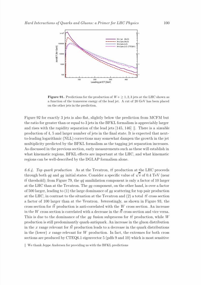
8/3/2019 Hard Interactions of Quarks and Gluons a Primer for LHC Physics
http://slidepdf.com/reader/full/hard-interactions-of-quarks-and-gluons-a-primer-for-lhc-physics 100/118
Hard Interactions of Quarks and Gluons: a Primer for LHC Physics 100
100 200 300 400
Leading jet ET [GeV]
100
1000
10000
100000
1x10⁶
d σ / d E T [ f b / G
e V ]
1
1
1
1
1
W+1 jet (NLO)
W+2 jets (NLO)
W+3 jets (LO)
W+3 jets (LO, CTEQ61)
Figure 91. Predictions for the production of W +
≥1, 2, 3 jets at the LHC shown as
a function of the transverse energy of the lead jet. A cut of 20 GeV has been placed
on the other jets in the prediction.
Figure 92 for exactly 3 jets is also flat, slightly below the prediction from MCFM but
the ratio for greater than or equal to 3 jets in the BFKL formalism is appreciably larger
and rises with the rapidity separation of the lead jets [145, 146] . There is a sizeable
production of 4, 5 and larger number of jets in the final state. It is expected that next-
to-leading logarithmic (NLL) corrections may somewhat dampen the growth in the jet
multiplicity predicted by the BFKL formalism as the tagging jet separation increases.
As discussed in the previous section, early measurements such as these will establish inwhat kinematic regions, BFKL effects are important at the LHC, and what kinematic
regions can be well-described by the DGLAP formalism alone.
6.6.4. Top quark production As at the Tevatron, tt production at the LHC proceeds
through both qq and gg initial states. Consider a specific value of √
s of 0.4 TeV (near
tt threshold); from Figure 79, the qq annihilation component is only a factor of 10 larger
at the LHC than at the Tevatron. The gg component, on the other hand, is over a factor
of 500 larger, leading to (1) the large dominance of gg scattering for top pair production
at the LHC, in contrast to the situation at the Tevatron and (2) a total tt cross section
a factor of 100 larger than at the Tevatron. Interestingly, as shown in Figure 93, the
cross section for tt production is anti-correlated with the W cross section. An increase
in the W cross section is correlated with a decrease in the tt cross section and vice versa.
This is due to the dominance of the gg fusion subprocess for tt production, while W
production is still predominantly quark-antiquark. An increase in the gluon distribution
in the x range relevant for tt production leads to a decrease in the quark distributions
in the (lower) x range relevant for W production. In fact, the extremes for both cross
sections are produced by CTEQ6.1 eigenvector 5 (pdfs 9 and 10) which is most sensitive
We thank Jeppe Andersen for providing us with the BFKL predictions
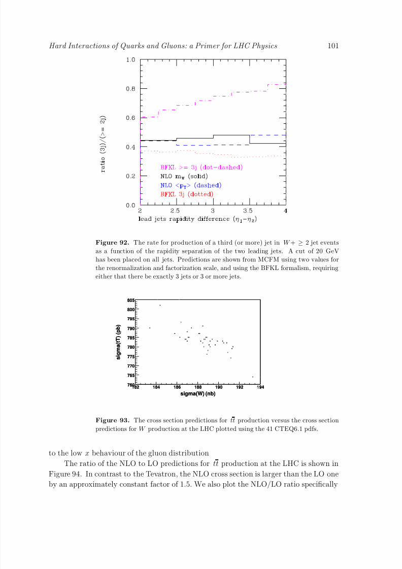
8/3/2019 Hard Interactions of Quarks and Gluons a Primer for LHC Physics
http://slidepdf.com/reader/full/hard-interactions-of-quarks-and-gluons-a-primer-for-lhc-physics 101/118
Hard Interactions of Quarks and Gluons: a Primer for LHC Physics 101
Figure 92. The rate for production of a third (or more) jet in W + ≥ 2 jet events
as a function of the rapidity separation of the two leading jets. A cut of 20 GeV
has been placed on all jets. Predictions are shown from MCFM using two values for
the renormalization and factorization scale, and using the BFKL formalism, requiring
either that there be exactly 3 jets or 3 or more jets.
sigma(W) (nb)
182 184 186 188 190 192 194
s i g m a ( t T ) ( p b )
760
765
770
775
780
785
790
795
800
805
ScaleT
Jet20 corrected Mulitple Interactions and Hadron P
sigma(W) (nb)
182 184 186 188 190 192 194
s i g m a ( t T ) ( p b )
760
765
770
775
780
785
790
795
800
805
Figure 93. The cross section predictions for tt production versus the cross section
predictions for W production at the LHC plotted using the 41 CTEQ6.1 pdfs.
to the low x behaviour of the gluon distribution
The ratio of the NLO to LO predictions for tt production at the LHC is shown in
Figure 94. In contrast to the Tevatron, the NLO cross section is larger than the LO one
by an approximately constant factor of 1.5. We also plot the NLO/LO ratio specifically
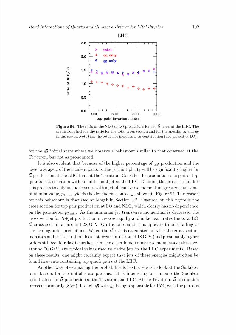
8/3/2019 Hard Interactions of Quarks and Gluons a Primer for LHC Physics
http://slidepdf.com/reader/full/hard-interactions-of-quarks-and-gluons-a-primer-for-lhc-physics 102/118
Hard Interactions of Quarks and Gluons: a Primer for LHC Physics 102
Figure 94. The ratio of the NLO to LO predictions for the tt mass at the LHC. The
predictions include the ratio for the total cross section and for the specific qq and gg
initial states. Note that the total also includes a gq contribution (not present at LO).
for the qq initial state where we observe a behaviour similar to that observed at the
Tevatron, but not as pronounced.
It is also evident that because of the higher percentage of gg production and the
lower average x of the incident partons, the jet multiplicity will be significantly higher for
tt production at the LHC than at the Tevatron. Consider the production of a pair of topquarks in association with an additional jet at the LHC. Defining the cross section for
this process to only include events with a jet of transverse momentum greater than some
minimum value, pT,min, yields the dependence on pT,min shown in Figure 95. The reason
for this behaviour is discussed at length in Section 3.2. Overlaid on this figure is the
cross section for top pair production at LO and NLO, which clearly has no dependence
on the parameter pT,min. As the minimum jet transverse momentum is decreased the
cross section for tt+jet production increases rapidly and in fact saturates the total LO
tt cross section at around 28 GeV. On the one hand, this appears to be a failing of
the leading order predictions. When the tt rate is calculated at NLO the cross section
increases and the saturation does not occur until around 18 GeV (and presumably higher
orders still would relax it further). On the other hand transverse momenta of this size,
around 20 GeV, are typical values used to define jets in the LHC experiments. Based
on these results, one might certainly expect that jets of these energies might often be
found in events containing top quark pairs at the LHC.
Another way of estimating the probability for extra jets is to look at the Sudakov
form factors for the initial state partons. It is interesting to compare the Sudakov
form factors for tt production at the Tevatron and LHC. At the Tevatron, tt production
proceeds primarily (85%) through qq with gg being responsible for 15%, with the partons

8/3/2019 Hard Interactions of Quarks and Gluons a Primer for LHC Physics
http://slidepdf.com/reader/full/hard-interactions-of-quarks-and-gluons-a-primer-for-lhc-physics 103/118
Hard Interactions of Quarks and Gluons: a Primer for LHC Physics 103
Figure 95. The dependence of the LO tt+jet cross section on the jet-defining
parameter pT,min, together with the top pair production cross sections at LO and
NLO.
(GeV/c)gluon
TP
10 15 20 25 30
S u d a k o v
f o r m f a
c t o r
0
0.2
0.4
0.6
0.8
1
ScaleT
Jet20 corrected Mulitple Interactions and Hadron P
(GeV/c)gluon
TP
10 15 20 25 30
S u d a k o v
f o r m f a
c t o r
0
0.2
0.4
0.6
0.8
1
Figure 96. The Sudakov form factors for initial state quarks and gluons at a hard
scale of 200 GeV as a function of the transverse momentum of the emitted gluon. The
form factors are for quarks (blue-solid) and gluons (red-dashed) at parton x values of
0.3 (crosses) and 0.03 (open circles).
evaluated near an average x value of 0.3. At the LHC, the percentages are roughly
reversed (or more precisely 90% for gg) and the scattering takes place at an average
x value of a factor of 7 lower (which we approximate here as x = 0.03). The relevant
Sudakov form factors are shown in Figure 96, as a function of the minimum transverse
momentum of the emitted gluon, at a hard scale of 200 GeV (roughly appropriate for
tt production). We can make some rough estimates from these plots. The probability
for no gluon of 10 GeV or greater to be radiated from an initial quark leg with x = 0.3
is 0.85. The probability for no such gluon to be radiated from either quark leg at the

8/3/2019 Hard Interactions of Quarks and Gluons a Primer for LHC Physics
http://slidepdf.com/reader/full/hard-interactions-of-quarks-and-gluons-a-primer-for-lhc-physics 104/118
Hard Interactions of Quarks and Gluons: a Primer for LHC Physics 104
Tevatron is 0.85 × 0.85 = 0.72, i.e. a 0.28 chance of radiating such a gluon. A similar
exercise for two incident gluons of x = 0.3 gives a chance of radiating a 10 GeV gluon of
0.51. As the qq initial state makes up 85% of the Tevatron cross section, with gg only
15%, the total probability of emitting at least one 10 GeV gluon is 0 .3. Using 90% for
gg at the LHC and 10% for qq, gives a 0.8 probability of radiating such a hard gluon.
The W +jets background to tt production proceeds primarily through the gq channel
and so receives a factor of 500 enhancement. Thus, the signal to background ratio for
tt production in a lepton + jets final state is significantly worse at the LHC than at
the Tevatron, if the same cuts on the jet transverse momenta as at the Tevatron are
used. Thus, the jet cuts applied to tt analyses at the LHC need to be set larger than
at the Tevatron in order, (1) to reduce the backgrounds from W + 4 jet production
relative to the lepton + 4 jets final state from tt decay, (2) to reduce the number of
jets produced by ISR in tt events, and (3) to reduce the likelihood of additional jets
produced by fluctuations in the underlying event. The signal to background for tt issubstantially improved at the LHC by increasing the minimum transverse momentum
cut for each jet from 15 GeV (Tevatron) to 30 GeV (CMS) or 40 GeV (ATLAS). The
cross section for the production of the lowest pT jet in W + 4 jet events falls roughly as
1/pnT (where n is in the range 2.5 − 3) while the distribution for the 4th jet transverse
momentum is essentially flat from 15–40 GeV. The background is reduced by a factor
of 15 while the signal is reduced by a factor of 5. This reduction in signal is acceptable
because of the large tt cross section available at the LHC. There are 2.5 million tt pairs
produced with a lepton + jets final state for a 10fb−1 data sample. The requirement for
two of the jets to be tagged as b-jets (and the kinematic cuts on the jets (40 GeV) and
on the lepton and missing transverse momentum) reduces the event sample to 87, 000,but with a signal to background ratio of 78. A requirement of only one b-tag reduces
the signal/background ratio to 28 but with a data sample a factor of 3 larger.
6.6.5. Higgs boson production As discussed in Section 2, the Higgs boson is the
cornerstone of the Standard Model and its supersymmetric extensions, and its discovery
will be one of the primary physics goals at the LHC. The Standard Model Higgs cross
sections for various production mechanisms are shown in Figure 97 (left) as a function
of the Higgs mass [147]. The branching ratios of the dominant decay modes for the
Standard Model Higgs boson are shown on the right side of the figure. The primaryproduction mechanism is through gg fusion and the primary decay mode is bb (low mass)
and W W (high mass).
Inclusive Higgs production through gg scattering is one of the few processes known
to NNLO. The rapidity distribution for Higgs boson production at the LHC is shown
in Figure 98 at LO, NLO and NNLO [69]. The NLO cross section is a factor of two
larger than the leading order cross section and the NNLO cross section is a factor of 20%
larger than the NLO one. The scale dependence at NNLO is of the order of 15%, so the
cross section uncertainties are under reasonable control. As observed in Figure 75, the
gg parton luminosity uncertainty is less than 10% over the expected Higgs mass range.
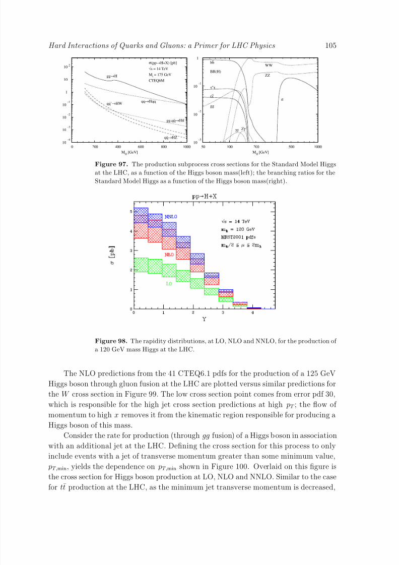
8/3/2019 Hard Interactions of Quarks and Gluons a Primer for LHC Physics
http://slidepdf.com/reader/full/hard-interactions-of-quarks-and-gluons-a-primer-for-lhc-physics 105/118
Hard Interactions of Quarks and Gluons: a Primer for LHC Physics 105
σ(pp→H+X) [pb]
√s = 14 TeV
Mt= 175 GeV
CTEQ6Mgg→H
qq→Hqqqq
_’→HW
qq_→HZ
gg,qq_→Htt
_
MH[GeV]
0 200 400 600 800 100010
-4
10-3
10-2
10-1
1
10
102
BR(H)
bb_
τ+τ−
cc_
gg
WW
ZZ
tt-
γγ Zγ
MH
[GeV]
50 100 200 500 100010
-3
10-2
10-1
1
Figure 97. The production subprocess cross sections for the Standard Model Higgs
at the LHC, as a function of the Higgs boson mass(left); the branching ratios for the
Standard Model Higgs as a function of the Higgs boson mass(right).
Figure 98. The rapidity distributions, at LO, NLO and NNLO, for the production of
a 120 GeV mass Higgs at the LHC.
The NLO predictions from the 41 CTEQ6.1 pdfs for the production of a 125 GeV
Higgs boson through gluon fusion at the LHC are plotted versus similar predictions for
the W cross section in Figure 99. The low cross section point comes from error pdf 30,which is responsible for the high jet cross section predictions at high pT ; the flow of
momentum to high x removes it from the kinematic region responsible for producing a
Higgs boson of this mass.
Consider the rate for production (through gg fusion) of a Higgs boson in association
with an additional jet at the LHC. Defining the cross section for this process to only
include events with a jet of transverse momentum greater than some minimum value,
pT,min, yields the dependence on pT,min shown in Figure 100. Overlaid on this figure is
the cross section for Higgs boson production at LO, NLO and NNLO. Similar to the case
for tt production at the LHC, as the minimum jet transverse momentum is decreased,
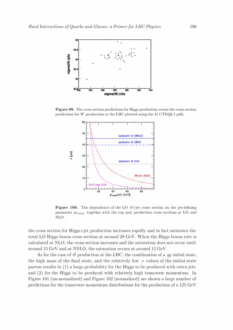
8/3/2019 Hard Interactions of Quarks and Gluons a Primer for LHC Physics
http://slidepdf.com/reader/full/hard-interactions-of-quarks-and-gluons-a-primer-for-lhc-physics 106/118
Hard Interactions of Quarks and Gluons: a Primer for LHC Physics 106
sigma(W) (nb)
182 184 186 188 190 192 194
s i g m a ( H ) ( p
b )
32.5
33
33.5
34
34.5
35
ScaleT
Jet20 corrected Mulitple Interactions and Hadron P
sigma(W) (nb)
182 184 186 188 190 192 194
s i g m a ( H ) ( p
b )
32.5
33
33.5
34
34.5
35
Figure 99. The cross section predictions for Higgs production versus the cross section
predictions for W production at the LHC plotted using the 41 CTEQ6.1 pdfs.
Figure 100. The dependence of the LO tt+jet cross section on the jet-defining
parameter pT,min, together with the top pair production cross sections at LO and
NLO.
the cross section for Higgs+jet production increases rapidly and in fact saturates thetotal LO Higgs boson cross section at around 28 GeV. When the Higgs boson rate is
calculated at NLO, the cross section increases and the saturation does not occur until
around 15 GeV and at NNLO, the saturation occurs at around 12 GeV.
As for the case of tt production at the LHC, the combination of a gg initial state,
the high mass of the final state, and the relatively low x values of the initial state
parton results in (1) a large probability for the Higgs to be produced with extra jets
and (2) for the Higgs to be produced with relatively high transverse momentum. In
Figure 101 (un-normalized) and Figure 102 (normalized) are shown a large number of
predictions for the transverse momentum distributions for the production of a 125 GeV

8/3/2019 Hard Interactions of Quarks and Gluons a Primer for LHC Physics
http://slidepdf.com/reader/full/hard-interactions-of-quarks-and-gluons-a-primer-for-lhc-physics 107/118
Hard Interactions of Quarks and Gluons: a Primer for LHC Physics 107
Figure 101. The predictions for the transverse momentum distribution for a 125 GeV
mass Higgs boson at the LHC from a number of theoretical predictions. The predictions
are shown with an absolute normalization. This figure can also be viewed in colour on
the benchmark website.
mass Higgs boson at the LHC, through the gg fusion process. The impact of higher
order corrections (both NLO and NNLO) on the normalization of the Higgs cross section
is evident in Figure 101. But in Figure 102, it can be observed that the shapes for the pT
distributions are basically the same. In particular, parton shower Monte Carlos provide
a reasonable approximation to the more rigorous predictions shown. Two PYTHIA
predictions are indicated: PYTHIA 6.215 is a virtuality-ordered parton shower while
PYTHIA 6.3 is a pT -ordered shower (and as different from PYTHIA 6.215 as HERWIG
is from PYTHIA). The peak of the PYTHIA 6.3 prediction is more in line with the
other theoretical predictions.
Note that the pT distribution of the Higgs boson peaks at approximately 12 GeV
while the pT distribution for the Z peaks at 3 GeV. The peak is slightly higher because
of the higher mass (125 GeV compared to 90 GeV) but the major shift is due to the
different production mechanisms. The colour factor for the gluon is greater than that
for the quark and the phase space available for gluon radiation for x = 0.01 gluons is

8/3/2019 Hard Interactions of Quarks and Gluons a Primer for LHC Physics
http://slidepdf.com/reader/full/hard-interactions-of-quarks-and-gluons-a-primer-for-lhc-physics 108/118
Hard Interactions of Quarks and Gluons: a Primer for LHC Physics 108
Figure 102. The predictions for the transverse momentum distribution for a 125 GeV
mass Higgs boson at the LHC from a number of theoretical predictions. The predictions
have all been normalized to the same cross section for shape comparisons. This figure
can also be viewed in colour on the benchmark website.
much larger due to the z → 0 pole in the splitting function.
The production of a Higgs boson through the vector boson fusion (VBF) process
is important, first of all, as a discovery channel and second, as a way of measuring
the Higgs couplings to W and Z bosons. There are backgrounds to this process from
(1) Higgs+2 jet production through gg fusion and (2) Z + 2 jet production, where the
Z decays into τ pairs (one of the primary search modes for Higgs production from
VBF) [179]. VBF production of a Higgs boson proceeds through the diagrams shown
in Figure 7. The emission of vector bosons from the initial state quark lines results
in the quarks acquiring a transverse momentum of the order of half of the W mass
(as the weak boson mass provides a natural cutoff for the weak boson propagator)
with a rapidity distribution peaked in the forward direction (the quarks still retain an
appreciable fraction of their original longitudinal momentum, corresponding to x values
of 0.1−−0.2). The two leading jets in Higgs+2 jets (from gg fusion) are peaked at central
rapidities as shown in Figure 103 and have a softer jet transverse momentum. Thus, a

8/3/2019 Hard Interactions of Quarks and Gluons a Primer for LHC Physics
http://slidepdf.com/reader/full/hard-interactions-of-quarks-and-gluons-a-primer-for-lhc-physics 109/118
Hard Interactions of Quarks and Gluons: a Primer for LHC Physics 109
Figure 103. The tagging jet η distributions in QCD H jj and VBF events. The band
indicates the range of predictions corresponding to variation of renormalization and
factorization scales by a factor of two about the central value of mH .
relatively hard cut on the tagging jet transverse momenta of 40 GeV and a requirement
that the tagging jets have large rapidity is effective at reducing the background without
a large impact on the VBF signal. The recent calculation of the Higgs+2 jet rate at
NLO [138] (one of the calculations on the wishlist) has somewhat ¶ reduced the scale
dependence, and thus the uncertainty, on the prediction +. The rate for additional jets
to be produced between the two tagging jets is high for the background processes [180].
The colourless exchange in the hard scattering in VBF leads to a suppression of extra
jets in the central rapidity region. Thus, as discussed earlier, a veto on extra jets in the
central region is effective at decreasing the background to VBF production of the Higgsboson.
6.6.6. Inclusive jet production The increase of the centre-of-mass energy to 14 TeV at
the LHC will result in a dramatically larger accessible kinematic range. Inclusive jet
cross sections can be measured out to transverse momentum values of order 4 TeV in the
central region and 1.5 TeV in the forward region. The predictions with the CTEQ6.1
central pdfs and the 40 error pdfs are shown in Figure 104 and 105 for three different
rapidity regions [11]. The cross sections were generated with a renormalization and
factorization scale equal to p jetT /2. The cross section predictions have a similar sensitivity
to the error pdfs as do the jet cross sections at the Tevatron for similar xT values, and
the uncertainties on the predicted cross sections remain up to a factor of 2 at the highest
pT values. Measurements of the jet cross section over the full rapidity range at the LHC
will serve to further constrain the high x gluon pdf and distinguish between possible
new physics and uncertainties in pdfs.
¶ The reduction of the scale dependence is not dramatic since there is a large contribution from the
(LO) Higgs+3 jet final state.+ It is interesting that the NLO corrections for Higgs+2 jets are relatively small, on the order of 20%.
This follows the pattern of the NLO corrections decreasing in size as the jet multiplicity increases; the
corrections are 80% for inclusive Higgs boson production (through gg fusion) and 50% for Higgs+1 jet.

8/3/2019 Hard Interactions of Quarks and Gluons a Primer for LHC Physics
http://slidepdf.com/reader/full/hard-interactions-of-quarks-and-gluons-a-primer-for-lhc-physics 110/118
Hard Interactions of Quarks and Gluons: a Primer for LHC Physics 110
Figure 104. Inclusive jet cross section predictions for the LHC using the CTEQ6.1
central pdf and the 40 error pdfs.
Figure 105. The ratios of the jet cross section predictions for the LHC using the
CTEQ6.1 error pdfs to the prediction using the central pdf. The extremes are produced
by eigenvector 15.
It is useful to plot the K -factors (the ratio of the NLO to LO cross sections)
for the three different rapidity intervals shown above. As discussed previously in
Section 3.3.3, the value of the K -factor is a scale-dependent quantity; the K -factors
shown in Figure 106 are calculated with the nominal scale of p jetT /2. The K -factors have
a somewhat complicated shape due to the interplay between the different subprocesses
comprising inclusive jet production and the behaviours of the relevant pdfs in the
different regions of parton momentum fraction x. In the central region, the K -factor

8/3/2019 Hard Interactions of Quarks and Gluons a Primer for LHC Physics
http://slidepdf.com/reader/full/hard-interactions-of-quarks-and-gluons-a-primer-for-lhc-physics 111/118
Hard Interactions of Quarks and Gluons: a Primer for LHC Physics 111
pT(GeV/c)0 1000 2000 3000 4000 5000
K - f a c t o r
0
0.2
0.4
0.6
0.8
1
1.2
1.4
1.6
Figure 106. The ratios of the NLO to LO jet cross section predictions for the LHC
using the CTEQ6.1 pdfs for the three different rapidity regions (0–1 (squares), 1–2
(triangles), 2–3 (circles)).
is within 10% of unity for the observable range. There are no new parton-parton
subprocesses that contribute at NLO but not at LO. Thus a LO prediction, using the
NLO CTEQ6.1 pdfs, will reproduce fairly closely the NLO calculation. For rapidities
between 1 and 2, the K -factor is within 20% of unity, dropping below one at higher
transverse momentum. For forward rapidities, the K -factor drops almost immediately
below one, due to the behaviour of the high-x pdfs that contribute to the cross section
in this region. There is nothing wrong with the NLO prediction in this region; its
relationship to the LO cross section has just changed due to the kinematics. LO
predictions in this region will provide an overestimate of the NLO cross section.
We saw in Section 5.3.1 that jets in the upper range of transverse momentum values
at the Tevatron were very collimated. This will be even more the case at the LHC, where
in the multi-TeV range, a large fraction of the jet’s momentum will be contained in a
single calorimeter tower. Jet events at the LHC will be much more active than events in a
similar pT range at the Tevatron. The majority of the dijet production for the transverse
momentum range less than 1 TeV will be with a gg initial state. As discussed previously,
the larger colour factor associated with the gluon and the greater phase space available
at the LHC for gluon emission will result in an increased production of additional soft
jets. In addition, there is an increased probability for the production of “mini-jets” frommultiple-parton scattering among the spectator partons. At full design luminosity, on
the order of 25 additional minimum bias interactions will be present at each crossing.
Such events, either singly or in combination, may create additional jets. As a result,
the minimum jet transverse momentum requirement may need to be increased for most
analyses; in addition, it may be advantageous to use smaller cone sizes than used for
similar analyses at the Tevatron.
As discussed above, the LHC will produce jets at transverse momenta far larger
than the W mass. Thus, virtual electroweak corrections of the form αW log2( p2T /M 2W ),
where αW = αEM sin2 θW , may become important. For example, at pT = 3 TeV,

8/3/2019 Hard Interactions of Quarks and Gluons a Primer for LHC Physics
http://slidepdf.com/reader/full/hard-interactions-of-quarks-and-gluons-a-primer-for-lhc-physics 112/118
Hard Interactions of Quarks and Gluons: a Primer for LHC Physics 112
Figure 107. The effect of electroweak logarithms on jet cross sections at the LHC.
log2( p2T /m2W ) = 10. These double logs are a result of the lack of cancellation between
real and virtual W emission in higher order calculations and may become competitive in
size with NLO QCD corrections. The impact of a subset of the full EW corrections (i.e.
those involving virtual electroweak boson emission only) reaches of the order of 40%
at 4 TeV, as shown in Figure 107 below [181]. This is an indication that all Standard
Model corrections, and not just those from higher order QCD, need to be understood
in order to correctly interpret any new physics that may be present at the LHC.
7. Summary
The LHC will present an unprecedented potential for the discovery of new physics. Thus,
it is even more important to understand both the possible production mechanisms for
the new physics and the Standard Model backgrounds for their signals. The experiences
gained at the Tevatron, and the phenomenological tools developed in the last few
years, will serve as a basis towards the establishment of the relevant Standard Model
benchmarks at the LHC. In this paper, we have put together a primer to aid this
establishment.
For convenience, we summarize below the rules-of-thumb and official recommenda-
tions discussed in our paper. First, the rules-of-thumb:
• In Section 3.3.3, we present K -factors for some important processes at the Tevatron
and the LHC.
• In Section 3.5.1, we present some plots of Sudakov form factors useful for calculating
the probability for producing jets from initial state radiation.
• In Section 6.2, we provide pdf luminosities and their uncertainties for the LHC.
Next, our official recommendations:
8/3/2019 Hard Interactions of Quarks and Gluons a Primer for LHC Physics
http://slidepdf.com/reader/full/hard-interactions-of-quarks-and-gluons-a-primer-for-lhc-physics 113/118
Hard Interactions of Quarks and Gluons: a Primer for LHC Physics 113
• In Section 4.4, we give our official recommendation for the form of the Master
Equation to be used to calculate pdf uncertainties.
• In Section 4.5, we recommend that NLO pdfs be used for Monte Carlo event
generations.• In Section 5.3.1, we recommend that experimental cross section measurements be
presented at the hadron level, and that corrections between the parton and hadron
levels be clearly stated.
• In Section 5.3.3, we present a revised version of the midpoint jet cone algorithm
and recommend its use at the Tevatron and LHC. We also recommend the use of
both cone and kT jet algorithms for all analyses.
Acknowledgements
We would like to thank J. Andersen, A. Belyaev, B. Cooper, A. de Roeck, L. Dixon,
S. Ellis, R. Field, S. Frixione, S. Gieseke, J. Heyninck, M. Mangano, A. Messina,
S. Mrenna, S. Moretti, I. Puljak, J. Pumplin, P. Skands, R. Thorne, M. Toennesmann
and S. Tsuno.
References
[1] S.D. Drell and T.M. Yan, Ann. Phys. 66 (1971) 578.
[2] J.C. Collins and D.E. Soper, Ann. Rev. Nucl. Part. Sci. 37 (1987) 33.
[3] V. Del Duca, W. Kilgore, C. Oleari, C. Schmidt and D. Zeppenfeld, Nucl. Phys. B 616 (2001) 367
[arXiv:hep-ph/0108030].[4] R. V. Harlander and W. B. Kilgore, Phys. Rev. Lett. 88, 201801 (2002) [arXiv:hep-ph/0201206].
[5] C. Anastasiou and K. Melnikov, Nucl. Phys. B 646, 220 (2002) [arXiv:hep-ph/0207004].
[6] D. Zeppenfeld, R. Kinnunen, A. Nikitenko and E. Richter-Was, Phys. Rev. D 62 (2000) 013009
[arXiv:hep-ph/0002036].
[7] A. Djouadi, arXiv:hep-ph/0503172.
[8] R. K. Ellis, W. J. Stirling and B. R. Webber, Camb. Monogr. Part. Phys. Nucl. Phys. Cosmol. 8,
1 (1996).
[9] L.N. Lipatov, Sov. J. Nucl. Phys. 20 (1975) 95;
V.N. Gribov and L.N. Lipatov, Sov. J. Nucl. Phys. 15 (1972) 438;
G. Altarelli and G. Parisi, Nucl. Phys. B126 (1977) 298;
Yu.L. Dokshitzer, Sov. Phys. JETP 46 (1977) 641.
[10] A. D. Martin, R. G. Roberts, W. J. Stirling and R. S. Thorne, Phys. Lett. B 604, 61 (2004)[arXiv:hep-ph/0410230].
[11] D. Stump, J. Huston, J. Pumplin, W. K. Tung, H. L. Lai, S. Kuhlmann and J. F. Owens, JHEP
0310, 046 (2003) [arXiv:hep-ph/0303013].
[12] D. Acosta et al. [CDF II Collaboration], Phys. Rev. Lett. 94, 091803 (2005) [arXiv:hep-
ex/0406078].
[13] http://www-d0.fnal.gov/Run2Physics/WWW/results/prelim/EW/
[14] S. D. Ellis, Z. Kunszt and D. E. Soper, Phys. Rev. Lett. 69, 3615 (1992) [arXiv:hep-ph/9208249].
[15] G. Corcella et al., JHEP 0101, 010 (2001) [arXiv:hep-ph/0011363].
[16] T. Sjostrand, S. Mrenna and P. Skands, JHEP 0605, 026 (2006) [arXiv:hep-ph/0603175].
[17] M. L. Mangano, M. Moretti and R. Pittau, Nucl. Phys. B 632, 343 (2002) [arXiv:hep-ph/0108069].

8/3/2019 Hard Interactions of Quarks and Gluons a Primer for LHC Physics
http://slidepdf.com/reader/full/hard-interactions-of-quarks-and-gluons-a-primer-for-lhc-physics 114/118
Hard Interactions of Quarks and Gluons: a Primer for LHC Physics 114
[18] M. L. Mangano, M. Moretti, F. Piccinini, R. Pittau and A. D. Polosa, JHEP 0307, 001 (2003)
[arXiv:hep-ph/0206293].
[19] A. Pukhov et al., arXiv:hep-ph/9908288.
[20] E. Boos et al. [CompHEP Collaboration], Nucl. Instrum. Meth. A 534, 250 (2004) [arXiv:hep-
ph/0403113].[21] T. Stelzer and W. F. Long, Comput. Phys. Commun. 81, 357 (1994) [arXiv:hep-ph/9401258].
[22] F. Maltoni and T. Stelzer, JHEP 0302, 027 (2003) [arXiv:hep-ph/0208156].
[23] F. Caravaglios, M. L. Mangano, M. Moretti and R. Pittau, Nucl. Phys. B 539, 215 (1999)
[arXiv:hep-ph/9807570].
[24] H. Murayama, I. Watanabe and K. Hagiwara, KEK-91-11
[25] F. Maltoni, K. Paul, T. Stelzer and S. Willenbrock, Phys. Rev. D 67, 014026 (2003) [arXiv:hep-
ph/0209271].
[26] E. Witten, Commun. Math. Phys. 252, 189 (2004) [arXiv:hep-th/0312171].
[27] F. Cachazo, P. Svrcek and E. Witten, JHEP 0409, 006 (2004) [arXiv:hep-th/0403047].
[28] G. Georgiou and V. V. Khoze, JHEP 0405, 070 (2004) [arXiv:hep-th/0404072].
[29] J. B. Wu and C. J. Zhu, JHEP 0409, 063 (2004) [arXiv:hep-th/0406146].
[30] G. Georgiou, E. W. N. Glover and V. V. Khoze, JHEP 0407, 048 (2004) [arXiv:hep-th/0407027].[31] L. J. Dixon, E. W. N. Glover and V. V. Khoze, JHEP 0412, 015 (2004) [arXiv:hep-th/0411092].
[32] S. D. Badger, E. W. N. Glover and V. V. Khoze, JHEP 0503, 023 (2005) [arXiv:hep-th/0412275].
[33] Z. Bern, D. Forde, D. A. Kosower and P. Mastrolia, Phys. Rev. D 72, 025006 (2005) [arXiv:hep-
ph/0412167].
[34] R. Britto, F. Cachazo and B. Feng, Nucl. Phys. B 715, 499 (2005) [arXiv:hep-th/0412308].
[35] R. Britto, F. Cachazo, B. Feng and E. Witten, Phys. Rev. Lett. 94, 181602 (2005) [arXiv:hep-
th/0501052].
[36] F. Bloch and A. Nordsieck, Phys. Rev. 52, 54 (1937).
[37] T. Kinoshita, J. Math. Phys. 3, 650 (1962).
[38] T. D. Lee and M. Nauenberg, Phys. Rev. 133, B1549 (1964).
[39] K. Kajantie, J. Lindfors and R. Raitio, Nucl. Phys. B 144, 422 (1978).
[40] Z. Kunszt and D. E. Soper, Phys. Rev. D 46, 192 (1992).[41] R. K. Ellis, D. A. Ross and A. E. Terrano, Nucl. Phys. B 178, 421 (1981).
[42] S. Frixione, Z. Kunszt and A. Signer, Nucl. Phys. B 467, 399 (1996) [arXiv:hep-ph/9512328].
[43] S. Catani and M. H. Seymour, Nucl. Phys. B 485, 291 (1997) [Erratum-ibid. B 510, 503 (1997)]
[arXiv:hep-ph/9605323].
[44] Z. Nagy and Z. Trocsanyi, Nucl. Phys. B 486, 189 (1997) [arXiv:hep-ph/9610498].
[45] K. Fabricius, I. Schmitt, G. Kramer and G. Schierholz, Z. Phys. C 11, 315 (1981).
[46] W. T. Giele and E. W. N. Glover, Phys. Rev. D 46, 1980 (1992).
[47] A. Gehrmann-De Ridder, T. Gehrmann and E. W. N. Glover, JHEP 0509, 056 (2005) [arXiv:hep-
ph/0505111].
[48] E. W. N. Glover and D. J. Miller, Phys. Lett. B 396, 257 (1997) [arXiv:hep-ph/9609474].
[49] Z. Bern, L. J. Dixon, D. A. Kosower and S. Weinzierl, Nucl. Phys. B 489, 3 (1997) [arXiv:hep-
ph/9610370].[50] J. M. Campbell, E. W. N. Glover and D. J. Miller, Phys. Lett. B 409, 503 (1997) [arXiv:hep-
ph/9706297].
[51] E. W. N. Glover, Nucl. Phys. Proc. Suppl. 116, 3 (2003) [arXiv:hep-ph/0211412].
[52] Z. Bern, L. J. Dixon and D. A. Kosower, Nucl. Phys. B 513, 3 (1998) [arXiv:hep-ph/9708239].
[53] S. D. Badger and E. W. N. Glover, JHEP 0407, 040 (2004) [arXiv:hep-ph/0405236].
[54] H1 Collaboration: C. Adloff et al., Eur. Phys. J. C 13 (2000) 609 [hep-ex/9908059]; Eur. Phys. J.
C 19 (2001) 269 [hep-ex/0012052]; Eur. Phys. J. C 21 (2001) 33 [hep-ex/0012053].
[55] ZEUS Collaboration: S. Chekanov et al., Eur. Phys. J. C 21 (2001) 443 [hep-ex/0105090]; A.M.
Cooper-Sarkar, Proceedings of International Europhysics Conference on HEP 2001, Budapest
[hep-ph/0110386].

8/3/2019 Hard Interactions of Quarks and Gluons a Primer for LHC Physics
http://slidepdf.com/reader/full/hard-interactions-of-quarks-and-gluons-a-primer-for-lhc-physics 115/118
Hard Interactions of Quarks and Gluons: a Primer for LHC Physics 115
[56] E866 Collaboration: R. S. Towell et al., Phys. Rev. D 64 (2001) 052002 [hep-ex/0103030].
[57] CCFR Collaboration: U. K. Yang et al., Phys. Rev. Lett. 86 (2001) 2742 [hep-ex/0009041].
[58] BCDMS Collaboration: A. C. Benvenuti et al., Phys. Lett. B 223 (1989) 485.
[59] BCDMS Collaboration: A. C. Benvenuti et al., Phys. Lett. B 236 (1989) 592.
[60] New Muon Collaboration: M. Arneodo et al., Nucl. Phys. B 483 (1997) 3 [hep-ph/9610231]; andM. Arneodo et al., Nucl. Phys. B 487 (1997) 3 [hep-ex/9611022].
[61] CCFR Collaboration: W. G. Seligman et al., Phys. Rev. Lett. 79 (1997) 1213 [hep-ex/970107].
[62] E605 Collaboration: G. Moreno et al., Phys. Rev. D 43 (1991) 2815.
[63] CDF Collaboration: T. Affolder et al., Phys. Rev. D 64 (2001) 032001 [hep-ph/0102074].
[64] DØ Collaboration: B. Abbott et al., Phys. Rev. Lett. 86 (2001) 1707 [hep-ex/0011036]; and Phys.
Rev. D 64 (2001) 032003 [hep-ex/0012046].
[65] S. Moch, J. A. M. Vermaseren and A. Vogt, Nucl. Phys. B 688, 101 (2004) [arXiv:hep-ph/0403192].
[66] A. Vogt, S. Moch and J. A. M. Vermaseren, Nucl. Phys. B 691, 129 (2004) [arXiv:hep-ph/0404111].
[67] R. Hamberg, W. L. van Neerven and T. Matsuura, Nucl. Phys. B 359, 343 (1991) [Erratum-ibid.
B 644, 403 (2002)].
[68] C. Anastasiou, L. J. Dixon, K. Melnikov and F. Petriello, Phys. Rev. Lett. 91, 182002 (2003)
[arXiv:hep-ph/0306192].[69] C. Anastasiou, K. Melnikov and F. Petriello, Phys. Rev. Lett. 93, 262002 (2004) [arXiv:hep-
ph/0409088].
[70] G. Sterman, Nucl. Phys. B 281, 310 (1987).
[71] S. Catani and L. Trentadue, Nucl. Phys. B 327, 323 (1989).
[72] S. Catani and L. Trentadue, Nucl. Phys. B 353, 183 (1991).
[73] G. Parisi and R. Petronzio, Nucl. Phys. B 154, 427 (1979).
[74] G. Altarelli, R. K. Ellis, M. Greco and G. Martinelli, Nucl. Phys. B 246, 12 (1984).
[75] J. C. Collins and D. E. Soper, Nucl. Phys. B 193, 381 (1981) [Erratum-ibid. B 213, 545 (1983)].
[76] J. C. Collins and D. E. Soper, Nucl. Phys. B 197, 446 (1982).
[77] J. C. Collins, D. E. Soper and G. Sterman, Nucl. Phys. B 250, 199 (1985).
[78] G. Sterman and W. Vogelsang, Phys. Rev. D 71, 014013 (2005) [arXiv:hep-ph/0409234].
[79] A. Kulesza, G. Sterman and W. Vogelsang, Phys. Rev. D 69, 014012 (2004) [arXiv:hep-ph/0309264].
[80] A. Kulesza, G. Sterman and W. Vogelsang, arXiv:hep-ph/0207148.
[81] C. Balazs and C. P. Yuan, Phys. Rev. D 56, 5558 (1997) [arXiv:hep-ph/9704258].
[82] A. Banfi, G. Corcella, M. Dasgupta, Y. Delenda, G. P. Salam and G. Zanderighi, arXiv:hep-
ph/0508096.
[83] S. Gieseke et al., arXiv:hep-ph/0609306.
[84] T. Gleisberg, S. Hoche, F. Krauss, A. Schalicke, S. Schumann and J. C. Winter, JHEP 0402, 056
(2004) [arXiv:hep-ph/0311263].
[85] T. Sjostrand and P. Z. Skands, Eur. Phys. J. C 39, 129 (2005) [arXiv:hep-ph/0408302].
[86] S. Gieseke, JHEP 0501, 058 (2005) [arXiv:hep-ph/0412342].
[87] G. C. Blazey et al., arXiv:hep-ex/0005012.
[88] W. T. Giele, E. W. N. Glover and D. A. Kosower, Phys. Rev. Lett. 73, 2019 (1994) [arXiv:hep-ph/9403347].
[89] S. D. Ellis, J. Huston and M. Tonnesmann, in Proc. of the APS/DPF/DPB Summer Study on
the Future of Particle Physics (Snowmass 2001) ed. N. Graf, eConf C010630, P513 (2001)
[arXiv:hep-ph/0111434].
[90] E. Boos et al., arXiv:hep-ph/0109068.
[91] S. Catani, F. Krauss, R. Kuhn and B. R. Webber, JHEP 0111, 063 (2001) [arXiv:hep-ph/0109231].
[92] T. Gleisberg, S. Hoeche, F. Krauss, A. Schaelicke, S. Schumann, G. Soff and J. Winter, Czech. J.
Phys. 55, B529 (2005) [arXiv:hep-ph/0409122].
[93] T. Q. W. Group et al., arXiv:hep-ph/0610012.
[94] S. Mrenna and P. Richardson, JHEP 0405, 040 (2004) [arXiv:hep-ph/0312274].

8/3/2019 Hard Interactions of Quarks and Gluons a Primer for LHC Physics
http://slidepdf.com/reader/full/hard-interactions-of-quarks-and-gluons-a-primer-for-lhc-physics 116/118
Hard Interactions of Quarks and Gluons: a Primer for LHC Physics 116
[95] Y. J. Chen, J. Collins and X. M. Zu, JHEP 0204, 041 (2002) [arXiv:hep-ph/0110257].
[96] J. C. Collins and X. Zu, JHEP 0503, 059 (2005) [arXiv:hep-ph/0411332].
[97] S. Frixione and B. R. Webber, JHEP 0206, 029 (2002) [arXiv:hep-ph/0204244].
[98] S. Frixione, P. Nason and B. R. Webber, JHEP 0308, 007 (2003) [arXiv:hep-ph/0305252].
[99] S. Frixione and B. R. Webber, arXiv:hep-ph/0506182.[100] Y. Kurihara, J. Fujimoto, T. Ishikawa, K. Kato, S. Kawabata, T. Munehisa and H. Tanaka, Nucl.
Phys. B 654, 301 (2003) [arXiv:hep-ph/0212216].
[101] M. Kramer and D. E. Soper, Phys. Rev. D 69, 054019 (2004) [arXiv:hep-ph/0306222].
[102] D. E. Soper, Phys. Rev. D 69, 054020 (2004) [arXiv:hep-ph/0306268].
[103] M. Kramer, S. Mrenna and D. E. Soper, Phys. Rev. D 73, 014022 (2006) [arXiv:hep-ph/0509127].
[104] Z. Nagy and D. E. Soper, JHEP 0510, 024 (2005) [arXiv:hep-ph/0503053].
[105] Z. Nagy and D. E. Soper, arXiv:hep-ph/0601021.
[106]
[106] S. Frixione, E. Laenen, P. Motylinski and B. R. Webber, arXiv:hep-ph/0512250.
[107] S. Alekhin, JETP Lett. 82, 628 (2005) [Pisma Zh. Eksp. Teor. Fiz. 82, 710 (2005)] [arXiv:hep-
ph/0508248].
[108] C. Adloff et al. [H1 Collaboration], Eur. Phys. J. C 21, 33 (2001) [arXiv:hep-ex/0012053].[109] C. Adloff et al. [H1 Collaboration], Eur. Phys. J. C 30, 1 (2003) [arXiv:hep-ex/0304003].
[110] S. Chekanov et al. [ZEUS Collaboration], Phys. Rev. D 67, 012007 (2003) [arXiv:hep-ex/0208023].
[111] S. Chekanov et al. [ZEUS Collaboration], Eur. Phys. J. C 42, 1 (2005) [arXiv:hep-ph/0503274].
[112] S. Moch, J. A. M. Vermaseren and A. Vogt, Nucl. Phys. Proc. Suppl. 135, 137 (2004) [arXiv:hep-
ph/0408075].
[113] A. D. Martin, R. G. Roberts, W. J. Stirling and R. S. Thorne, Phys. Lett. B 531, 216 (2002)
[arXiv:hep-ph/0201127].
[114] M. Gluck, E. Reya and A. Vogt, Eur. Phys. J. C 5, 461 (1998) [arXiv:hep-ph/9806404].
[115] F. Abe et al. [CDF Collaboration], Phys. Rev. Lett. 81, 5754 (1998) [arXiv:hep-ex/9809001].
[116] D. Stump et al., Phys. Rev. D 65, 014012 (2002) [arXiv:hep-ph/0101051].
[117] J. Pumplin et al., Phys. Rev. D 65, 014013 (2002) [arXiv:hep-ph/0101032].
[118] A. D. Martin, R. G. Roberts, W. J. Stirling and R. S. Thorne, Eur. Phys. J. C 28, 455 (2003)[arXiv:hep-ph/0211080].
[119] S. Eidelman et al. [Particle Data Group], Phys. Lett. B 592, 1 (2004).
[120] J. Pumplin, A. Belyaev, J. Huston, D. Stump and W. K. Tung, JHEP 0602, 032 (2006)
[arXiv:hep-ph/0512167].
[121] J. C. Collins and X. m. Zu, JHEP 0206, 018 (2002) [arXiv:hep-ph/0204127].
[122] H. Plothow-Besch, Int. J. Mod. Phys. A 10, 2901 (1995).
[123] W. T. Giele, S. A. Keller and D. A. Kosower, arXiv:hep-ph/0104052.
[124] W. Giele et al., arXiv:hep-ph/0204316.
[125] M. R. Whalley, D. Bourilkov and R. C. Group, arXiv:hep-ph/0508110.
[126] J. M. Campbell and R. K. Ellis, Phys. Rev. D 62, 114012 (2000) [arXiv:hep-ph/0006304].
[127] A. Abulencia et al. [CDF Collaboration], Phys. Rev. D 73, 032003 (2006) [arXiv:hep-ex/0510048].
[128] G. J. Alner et al. [UA5 Collaboration], Phys. Rept. 154, 247 (1987).[129] C. Anastasiou, L. J. Dixon, K. Melnikov and F. Petriello, Phys. Rev. D 69, 094008 (2004)
[arXiv:hep-ph/0312266].
[130] See http://www-cdf.fnal.gov/physics/new/qcd/QCD.html.
[131] D. Acosta et al. [CDF Collaboration], Phys. Rev. D 70, 072002 (2004) [arXiv:hep-ex/0404004].
[132]
[132] A. A. Affolder et al. [CDF Collaboration], Phys. Rev. D 65, 092002 (2002).
[133] S. D. Ellis, Z. Kunszt and D. E. Soper, Phys. Rev. Lett. 64, 2121 (1990).
[134] D. Acosta et al. [CDF Collaboration], arXiv:hep-ex/0505013.
[135] A. Abulencia et al. [CDF Run II Collaboration], arXiv:hep-ex/0512020.
[136] A. Abulencia et al. [CDF II Collaboration], Phys. Rev. Lett. 96, 122001 (2006) [arXiv:hep-
8/3/2019 Hard Interactions of Quarks and Gluons a Primer for LHC Physics
http://slidepdf.com/reader/full/hard-interactions-of-quarks-and-gluons-a-primer-for-lhc-physics 117/118
Hard Interactions of Quarks and Gluons: a Primer for LHC Physics 117
ex/0512062].
[137] D. Acosta et al. [CDF Collaboration], Phys. Rev. D 71, 052003 (2005) [arXiv:hep-ex/0410041].
[138] J. M. Campbell, R. Keith Ellis and G. Zanderighi, arXiv:hep-ph/0608194.
[139] J. Campbell and J. Huston, Phys. Rev. D 70, 094021 (2004).
[140] D. Acosta et al. [CDF Collaboration], Phys. Rev. D 72, 052003 (2005) [arXiv:hep-ex/0504053].[141] http://www-cdf.fnal.gov/physics/new/top/2006/xs ann/public.html
[142] http : //www − cdf.fnal.gov/physics/new/top/2006/xs ljetsvx/public.html
[143] http://tevewwg.fnal.gov/top/
[144] C. T. Hill and E. H. Simmons, Phys. Rept. 381, 235 (2003) [Erratum-ibid. 390, 553 (2004)]
[arXiv:hep-ph/0203079].
[145] J. R. Andersen, V. Del Duca, F. Maltoni and W. J. Stirling, JHEP 0105, 048 (2001) [arXiv:hep-
ph/0105146].
[146] J. R. Andersen, Phys. Lett. B 639, 290 (2006) [arXiv:hep-ph/0602182].
[147] http://cms.cern.ch/iCMS/
[148] http://atlas.web.cern.ch/Atlas/GROUPS/PHYSICS/TDR/access.html
[149] C. Buttar et al., arXiv:hep-ph/0604120.
[150] A. Pukhov, arXiv:hep-ph/0412191.[151] S. Alekhin, [arXiv:hep-ph/0311184]; Phys. Rev. D 68, 014002 (2003) [arXiv:hep-ph/0211096].
[152] A. D. Martin, R. G. Roberts, W. J. Stirling and R. S. Thorne, Eur. Phys. J. C 35, 325 (2004)
[arXiv:hep-ph/0308087].
[153] A. D. Martin, R. G. Roberts, W. J. Stirling and R. S. Thorne, Phys. Lett. B 531, 216 (2002)
[arXiv:hep-ph/0201127].
[154] J. Huston, J. Pumplin, D. Stump and W. K. Tung, JHEP 0506, 080 (2005) [arXiv:hep-
ph/0502080].
[155] Z. Bern, L. J. Dixon and D. A. Kosower, Ann. Rev. Nucl. Part. Sci. 46, 109 (1996) [arXiv:hep-
ph/9602280].
[156] F. Cachazo, P. Svrcek and E. Witten, JHEP 0410, 074 (2004) [arXiv:hep-th/0406177].
[157] A. Brandhuber, B. J. Spence and G. Travaglini, Nucl. Phys. B 706, 150 (2005) [arXiv:hep-
th/0407214].[158] A. Brandhuber, S. McNamara, B. J. Spence and G. Travaglini, JHEP 0510, 011 (2005)
[arXiv:hep-th/0506068].
[159] Z. Bern, L. J. Dixon and D. A. Kosower, Phys. Rev. D 71, 105013 (2005) [arXiv:hep-th/0501240].
[160] D. Forde and D. A. Kosower, arXiv:hep-ph/0509358.
[161] A. Ferroglia, M. Passera, G. Passarino and S. Uccirati, Nucl. Phys. B 650, 162 (2003) [arXiv:hep-
ph/0209219].
[162] C. Anastasiou and A. Daleo, arXiv:hep-ph/0511176.
[163] W. T. Giele and E. W. N. Glover, JHEP 0404, 029 (2004) [arXiv:hep-ph/0402152].
[164] W. Giele, E. W. N. Glover and G. Zanderighi, Nucl. Phys. Proc. Suppl. 135, 275 (2004)
[arXiv:hep-ph/0407016].
[165] F. del Aguila and R. Pittau, JHEP 0407, 017 (2004) [arXiv:hep-ph/0404120].
[166] A. van Hameren, J. Vollinga and S. Weinzierl, Eur. Phys. J. C 41, 361 (2005) [arXiv:hep-ph/0502165].
[167] T. Binoth, J. P. Guillet, G. Heinrich, E. Pilon and C. Schubert, JHEP 0510, 015 (2005)
[arXiv:hep-ph/0504267].
[168] R. K. Ellis, W. T. Giele and G. Zanderighi, arXiv:hep-ph/0508308.
[169] R. K. Ellis, W. T. Giele and G. Zanderighi, Phys. Rev. D 72, 054018 (2005) [arXiv:hep-
ph/0506196].
[170] G. U. Flanagan, FERMILAB-THESIS-2005-58
[171] C. Balazs, J. Huston and I. Puljak, Phys. Rev. D 63, 014021 (2001) [arXiv:hep-ph/0002032].
[172] J. C. Collins, D. E. Soper and G. Sterman, Nucl. Phys. B 263, 37 (1986).
[173] S. Berge, P. Nadolsky, F. Olness and C. P. Yuan, Phys. Rev. D 72, 033015 (2005) [arXiv:hep-

8/3/2019 Hard Interactions of Quarks and Gluons a Primer for LHC Physics
http://slidepdf.com/reader/full/hard-interactions-of-quarks-and-gluons-a-primer-for-lhc-physics 118/118
Hard Interactions of Quarks and Gluons: a Primer for LHC Physics 118
ph/0410375].
[174] V. S. Fadin, E. A. Kuraev and L. N. Lipatov, Phys. Lett. B 60, 50 (1975).
[175] E. A. Kuraev, L. N. Lipatov and V. S. Fadin, Sov. Phys. JETP 44, 443 (1976) [Zh. Eksp. Teor.
Fiz. 71, 840 (1976)].
[176] E. A. Kuraev, L. N. Lipatov and V. S. Fadin, Sov. Phys. JETP 45, 199 (1977) [Zh. Eksp. Teor.Fiz. 72, 377 (1977)].
[177] I. I. Balitsky and L. N. Lipatov, Sov. J. Nucl. Phys. 28, 822 (1978) [Yad. Fiz. 28, 1597 (1978)].
[178] S. Berge, P. M. Nadolsky, F. I. Olness and C. P. Yuan, AIP Conf. Proc. 792, 722 (2005)
[arXiv:hep-ph/0508215].
[179] E. L. Berger and J. Campbell, Phys. Rev. D 70, 073011 (2004) [arXiv:hep-ph/0403194].
[180]
[180] V. Del Duca, A. Frizzo and F. Maltoni, JHEP 0405, 064 (2004) [arXiv:hep-ph/0404013].
[181] S. Moretti, M. R. Nolten and D. A. Ross, arXiv:hep-ph/0503152.