Sea level and global ice volumes from the Last GlacialMaximum to the HoloceneKurt Lambecka,b,1, Hélène Roubya,b, Anthony Purcella, Yiying Sunc, and Malcolm Sambridgea

aResearch School of Earth Sciences, The Australian National University, Canberra, ACT 0200, Australia; bLaboratoire de Géologie de l’École NormaleSupérieure, UMR 8538 du CNRS, 75231 Paris, France; and cDepartment of Earth Sciences, University of Hong Kong, Hong Kong, China

This contribution is part of the special series of Inaugural Articles by members of the National Academy of Sciences elected in 2009.

Contributed by Kurt Lambeck, September 12, 2014 (sent for review July 1, 2014; reviewed by Edouard Bard, Jerry X. Mitrovica, and Peter U. Clark)

The major cause of sea-level change during ice ages is the exchangeof water between ice and ocean and the planet’s dynamic responseto the changing surface load. Inversion of ∼1,000 observations forthe past 35,000 y from localities far from former ice margins hasprovided new constraints on the fluctuation of ice volume in thisinterval. Key results are: (i) a rapid final fall in global sea level of∼40 m in <2,000 y at the onset of the glacial maximum ∼30,000 ybefore present (30 ka BP); (ii) a slow fall to −134 m from 29 to 21 kaBP with a maximum grounded ice volume of ∼52 × 106 km3 greaterthan today; (iii) after an initial short duration rapid rise and a shortinterval of near-constant sea level, the main phase of deglaciationoccurred from ∼16.5 ka BP to ∼8.2 ka BP at an average rate of riseof 12 m·ka−1 punctuated by periods of greater, particularly at 14.5–14.0 ka BP at ≥40 mm·y−1 (MWP-1A), and lesser, from 12.5 to11.5 ka BP (Younger Dryas), rates; (iv) no evidence for a globalMWP-1B event at ∼11.3 ka BP; and (v) a progressive decrease inthe rate of rise from 8.2 ka to ∼2.5 ka BP, after which ocean vol-umes remained nearly constant until the renewed sea-level rise at100–150 y ago, with no evidence of oscillations exceeding ∼15–20 cm in time intervals ≥200 y from 6 to 0.15 ka BP.

sea level | ice volumes | Last Glacial Maximum | Holocene

The understanding of the change in ocean volume during gla-cial cycles is pertinent to several areas of earth science: for

estimating the volume of ice and its geographic distributionthrough time (1); for calibrating isotopic proxy indicators ofocean volume change (2, 3); for estimating vertical rates of landmovement from geological data (4); for examining the responseof reef development to changing sea level (5); and for recon-structing paleo topographies to test models of human and othermigrations (6). Estimates of variations in global sea level comefrom direct observational evidence of past sea levels relativeto present and less directly from temporal variations in theoxygen isotopic signal of ocean sediments (7). Both yield model-dependent estimates. The first requires assumptions about pro-cesses that govern how past sea levels are recorded in the coastalgeology or geomorphology as well as about the tectonic, isostatic,and oceanographic contributions to sea level change. The secondrequires assumptions about the source of the isotopic or chemicalsignatures of marine sediments and about the relative importanceof growth or decay of the ice sheets, of changes in ocean andatmospheric temperatures, or from local or regional factors thatcontrol the extent and time scales of mixing within ocean basins.Both approaches are important and complementary. The direct

observational evidence is restricted to time intervals or climatic andtectonic settings that favor preservation of the records throughotherwise successive overprinting events. As a result, the recordsbecome increasingly fragmentary backward in time. The isotopicevidence, in contrast, being recorded in deep-water carbonatemarine sediments, extends further back in time and often yieldsnear-continuous records of high but imprecise temporal resolution(8). However, they are also subject to greater uncertainty becauseof the isotope signal’s dependence on other factors. Comparisons

for the Holocene for which the direct measures of past sea level arerelatively abundant, for example, exhibit differences both in phaseand in noise characteristics between the two data [compare, forexample, the Holocene parts of oxygen isotope records from thePacific (9) and from two Red Sea cores (10)].Past sea level is measured with respect to its present position

and contains information on both land movement and changes inocean volume. During glacial cycles of ∼105 y, the most importantcontribution with a global signature is the exchange of mass be-tween the ice sheets and oceans, with tectonic vertical landmovements being important mainly on local and regional scales.Global changes associated with mantle convection and surfaceprocesses are comparatively small on these time scales but be-come important in longer, e.g., Pliocene-scale, periods (11).Changes in ocean volume associated with changing ocean tem-peratures during a glacial period are also small (12).The sea-level signal from the glacial cycle exhibits significant

spatial variability from its globally averaged value because of thecombined deformation and gravitational response of the Earthand ocean to the changing ice-water load. During ice-sheet de-cay, the crust rebounds beneath the ice sheets and subsides be-neath the melt-water loaded ocean basins; the gravitationalpotential and ocean surface are modified by the deformation andchanging surface load; and the planet’s inertia tensor and rota-tion changes, further modifying equipotential surfaces. Together,this response of the earth-ocean system to glacial cycles is re-ferred to as the glacial isostatic adjustment (GIA) (13–17). Thepattern of the spatial variability is a function of the Earth’srheology and of the glacial history, both of which are only partlyknown. In particular, past ice thickness is rarely observed and

Significance

Several areas of earth science require knowledge of the fluctua-tions in sea level and ice volume through glacial cycles. These in-clude understanding past ice sheets and providing boundaryconditions for paleoclimate models, calibrating marine-sedimentisotopic records, and providing the background signal for evalu-ating anthropogenic contributions to sea level. From ∼1,000observations of sea level, allowing for isostatic and tectonic con-tributions, we have quantified the rise and fall in global ocean andice volumes for the past 35,000 years. Of particular note is thatduring the ∼6,000 y up to the start of the recent rise ∼100−150 yago, there is no evidence for global oscillations in sea level on timescales exceeding ∼200 y duration or 15−20 cm amplitude.

Author contributions: K.L. designed research; K.L., H.R., A.P., Y.S., and M.S. performedresearch; Y.S. contributed field data; K.L., H.R., A.P., Y.S., and M.S. analyzed data; K.L. andH.R. wrote the paper; and A.P. and M.S. developed software.

Reviewers: E.B., CEREGE; J.X.M., Harvard University; and P.U.C., Oregon State University.

The authors declare no conflict of interest.

Freely available online through the PNAS open access option.1To whom correspondence should be addressed. Email: kurt.lambeck@anu.edu.au.

This article contains supporting information online at www.pnas.org/lookup/suppl/doi:10.1073/pnas.1411762111/-/DCSupplemental.

15296–15303 | PNAS | October 28, 2014 | vol. 111 | no. 43 www.pnas.org/cgi/doi/10.1073/pnas.1411762111

questions remain about the timing and extent of the former icesheets on the continental shelves. The sea-level response within,or close to, the former ice margins (near-field) is primarily afunction of the underlying rheology and ice thickness while, farfrom the former ice margins (far-field), it is mainly a function ofearth rheology and the change in total ice volume through time.By an iterative analysis of observational evidence of the past sealevels, it becomes possible to improve the understanding of thepast ice history as well as the Earth’s mantle response to forceson a 104 y to 105 y time scale.In this paper, we address one part of the Earth’s response to

the glacial cycle: the analysis of far-field evidence of sea-levelchange to estimate the variation in ice and ocean volumes fromthe lead into the Last Glacial Maximum (LGM) at ∼35,000 y ago(35 ka BP) to the start of the instrumental records. Such analysescan either be of high-resolution records of a single data typefrom a single location or of different sea-level indicators frommany different locations. We have adopted the latter approach.Most sea-level indicators provide only lower (e.g., fossil coral) orupper (e.g., fossil terrestrial plants) limiting values, and multipledata-type analyses of both upper and lower limiting measure-ments are less likely to be biased toward one or the other limit.Tectonic displacement of the crust is always a potential con-taminator of the sought signal, and a multiplicity of data fromtectonically “stable” regions is more likely to average out anyundetected tectonic effects as well as any uncertainties in theabove-mentioned GIA contributions.

Analysis StrategyIn a zero-order approximation, the change in sea level duringglacial cycles is the ice-volume equivalent sea level (esl) Δζesldefined as

ΔζeslðtÞ=−1ρo

Zt

1AoðtÞ

dΔMice

dtdt [1]

where ΔMice is the change in ice mass on the continents andgrounded on the shelves at time t with respect to present, Ao isthe ocean area defined by the coastline and ice grounding line att, and ρo is the average density of the ocean. Superimposed onthis is the response of the earth and ocean surface to the changesin loading. Hence, as a first approximation, the relative sea-levelΔζrsl at a location ϕ and time t is

Δζrslðϕ; tÞ=ΔζeslðtÞ+ δζisoiceðϕ; tÞ+ δζisowaterðϕ; tÞ [2]

where δζisoiceðϕ; tÞ and δζisowaterðϕ; tÞ are the isostatic contributionsfrom the changing ice and water loads, respectively. Because ofthe direct gravitational attraction of the ice sheets and deforma-tion of the ocean basin during the glacial cycle, δζisowaterðϕ; tÞ is notindependent of ice sheet geometry. Consequently, higher-orderiterative solutions are necessary to solve [2].In the absence of tectonics, the dominant departure of far-field

sea level from its global mean [1] is due to δζisowaterðϕ; tÞ and resultsin a strong spatial variability of Δζrslðϕ; tÞ across continentalmargins and within partially enclosed ocean basins that is de-pendent on mantle rheology, the amount of water added into theoceans, and the rate at which it is discharged, but is relativelyinsensitive to where this melt water originated. Typically, duringthe melting phase, δζisowaterðϕ; tÞ is about 15–25% of ΔζeslðtÞ andleads to near-coastal observations of LGM sea level beingsystematically less than the corresponding ΔζeslðtÞ. When de-glaciation ceases, the seafloor continues to deform because of theviscous nature of the mantle, and sea levels particularly at conti-nental edges fall slowly until all load stresses have relaxed. Thismechanism often produces small highstands at ∼5–7 ka BP thatmark the end of the dominant melting period (15, 16, 18).

The δζisoiceðϕ; tÞ reflects mantle-scale flow induced by the changesin ice load. This signal includes the evolution of a broad troughand bulge system that extends several thousand kilometers be-yond the ice margin, as a combined result of surface deformationand gravitational potential change (the “geoidal” bulge). Beyondthese features, δζisoiceðϕ; tÞ shows less spatial variability thanδζisowaterðϕ; tÞ and is relatively insensitive to the details of the iceload, but the amplitudes of these signals are not negligible andare earth-rheology dependent.The challenge is, in the presence of imperfect and incomplete

data, to invert the complete formulation of [2] for both the earthand ice unknowns. This challenge is approached here through thefollowing iterative procedure: (i) Start with far-field sea-level data,assume Δζrsl =Δζesl and using [1] estimate a first approximation ofice mass or volume function ΔViceðtÞ. (ii) Distribute this ice be-tween the known ice sheets, guided by either published in-formation or by glaciological hypotheses and with ice advance andretreat histories, depending on the state of knowledge of theparticular ice sheet. (iii) Invert far-field sea-level data for earthrheology parameters E (mantle viscosity, elastic thickness of thelithosphere) and for a corrective term δζesl to the nominal Δζ0eslcorresponding to step ii, yielding an improved approximation ofice volume function ΔViceðtÞ. (iv) Analyze sea-level data separatelyfor each of the major ice sheets (near-field analyses) and, startingwith the ice models from step ii, invert for both E and correctionsto ice-thickness functions I. (v) Impose the condition that the sumof the individual ice volume functions equals ΔViceðtÞ from step iiiand distribute any discrepancies between the ice sheets. (vi) Re-peat steps iii–v until convergence has been achieved.Advantages of this approach include the ability to analyze

individual ice sheets with different resolutions depending on thestate of a priori knowledge of the ice sheet and quality of theobservational data, as well as to make a first-order estimate forlateral variation in mantle viscosity.

Observational EvidenceThe principal sources for quantitative sea-level information arefrom sediment and coral records whose depositional environ-ments relative to mean sea level (MSL) are assumed known andwhose ages have been determined either by radiocarbon or ura-nium-series dating. In the former case, all 14C ages have beencalibrated using either the calibrations provided by the originalauthors or the IntCal09 calibration (19). Reservoir and isotopicfractionation corrections have been applied where appropriate.Corals provide lower-limit estimates of mean-low-water-spring

(MLWS) tide, but their growth depth range δζd is species andenvironment dependent (20). Assuming that the modern range isrepresentative of the past growth range, the adopted mean sealevel from in situ fossil corals of age t at elevation ζ (all verticalmeasures are positive upward) is

Δζrslðϕ; tÞ= ζðϕ; tÞ− δζd=2− δζtide

where δζtide is the MLWS level with respect to MSL (with thefurther assumption that, in the absence of paleo tide amplitudeinformation, there has been no significant change in tides). Theadopted precision estimate of the observation is Δζd/2, added inquadrature to other error sources. Greater uncertainties canarise at times of very rapid sea-level rise if reef formation cannotkeep up. In some special morphological forms, the in situ coralcan be related more directly to MLWS, as is the case of micro-atolls where the coral grows up to this limiting level before grow-ing radially outward at the MLWS level (21). Observed recordsare restricted to the past ∼6–7 ka, when far-field sea-level changewas slow enough for the microatoll development to be able tokeep up with change (22). The most complete record is fromKiritimati Atoll (23). The principal coral records for the lateglacial period are from Barbados (24–26), Tahiti (27, 28), Huon

Lambeck et al. PNAS | October 28, 2014 | vol. 111 | no. 43 | 15297

EART

H,A

TMOSP

HER

IC,

ANDPL

ANET

ARY

SCIENCE

SINAUGURA

LART

ICLE

Peninsula of Papua New Guinea (29, 30), the western Indian Ocean(31), and the Great Barrier Reef of Australia, supplemented for thepast 7 ka with other observations from the Australian region andthe Indian Ocean (Fig. 1 and SI Appendix, Table S1).The sedimentological evidence consists of age−depth relation-

ships of material formed within a known part of the tidal range,such as terrestrial plants representative of the highest tidal zone ormicrofaunal material representative of a lower tidal range (32)(observations that provide only limiting estimates have been ex-cluded). This evidence has the ability to provide high-precisionresults if restricted to materials with well-understood depositionalranges, but they also present their own difficulties. Is the datedmaterial within the sediment layer in situ? Has there been agecontamination by transport of older carbon into the sediment se-quence? Has compaction of the sediment column subsequent to

deposition been important? Significant data sources included arefrom the Sunda Shelf (33, 34), the Indian Ocean (35, 36), theBonaparte Gulf (37, 38), New Zealand (39), Singapore (40, 41),Malaysia (42), and from the SouthChina Sea to theBohai Sea.Manyof the Asian observations are from large delta systems, and com-parisons of such data with observations from adjacent sites oftenindicate lower levels of the former, corresponding to differentialsubsidence rates of the order of 1 mm·y−1 for the past ∼8 ka. Hencedata from the deltas of Chao Phraya of Thailand, Mekong and Redrivers of northern Vietnam, and Pearl and Yangtze rivers of China,have not been used for the purpose of estimating the esl function.Where possible, the selected data are from tectonically stable

regions: away from plate margins and marked by an absence ofseismic activity and recent faulting. Where available, evidence forthe Last Interglacial (marine isotope stage 5.5) shoreline, formedwhen, globally, sea levels were ∼4–8 m above present (43, 44), hasbeen used to assess the long-term stability of the region or tocorrect for tectonic displacement. Both Huon Peninsula andBarbados have been subject to uplift, and Tahiti to subsidence (SIAppendix, Text S1). The eastern Asian margin in many locationsis characterized by rifting of Cenozoic age and postrift thermalsubsidence (45), but the expected rates are small on time scales ofthe past 20 ka compared with the GIA signals and observationaluncertainties, and no corrections have been applied.

Inversion Results: Mantle RheologyThe observation equation is

Δζobsðϕ; tÞ+ «obs =Δζpredictedðϕ; tÞ=Δζ0eslðtÞ+ δζeslðtÞ+ δζisoiceðϕ; tÞ+ δζisowaterðϕ; tÞ

[3]

where «obs are corrections to the observations of relative sea leveland δζeslðtÞ is a corrective term to Δζ0eslðtÞ, parameterized in thefirst instance as mean values in time bins of 1,000 y from presentto 22 ka BP, with larger bins for the data-sparse intervals 22–26 ka BP, 26–31 ka BP, and 31–36 ka BP (Fig. 1). The inversionfor the earth-model parameters E and δζeslðtÞ is by forward mod-eling through E space in which for any Ek (k = 1. . .K), thecorresponding δζk;eslðtÞ is estimated by weighted least squares.The minimum value of the variance function Ψ2

k in E space,

Ψ2k =

1M

XMm=1

��Δζmobs −

�Δζ0esl + δζk;esl + δζk;iso

���σm�2

; [4]

is then sought, where δζk;iso is the total isostatic correction for Ekand σm is the SD of themth observation (m = 1. . .M). The E spaceis initially restricted to a three-layered model of the mantle: elasticlithosphere (including the crust) defined by an effective elasticthickness H, upper mantle from the base of the lithosphere tothe 670 km seismic discontinuity with a depth-averaged effectiveviscosity ηum, and a lower mantle viscosity extending down to thecore-mantle boundary of depth-averaged effective viscosity ηlm.Elastic moduli and density are based on realistic depth profilesdetermined from seismic data inversions. These approximate mod-els nevertheless describe well the response of the Earth to surfaceloading at periods and mantle-lithosphere stress levels of glacialcycles (46, 47). The E search is conducted within the confines

Effective lithospheric thickness: 30≤H1 ≤ 140 km:Effective upper-mantle viscosity: 1019 ≤ ηum ≤ 1021 Pa s:Effective lower-mantle viscosity: 5× 1020 ≤ ηlm ≤ 1024 Pa s:

[5]

that span parameters found in earlier far- and near-field analyses.The theory for the viscoelastic solution of earth deformation is

Fig. 1. Distribution of far-field sea-level data for the past 35 ka. (A) Depth−age relationship of all data with 2σ error estimates. (B) Time distribution of thedata. (C) Geographic distribution of all far-field coral (red dot) and sediment(black triangles) data.

15298 | www.pnas.org/cgi/doi/10.1073/pnas.1411762111 Lambeck et al.

based on the transformation of the elastic formulation into theLaplace domain using the correspondence principle and theninverting the Laplace-domain solution back into the time domain(13, 15, 48). This latter inversion is carried out using a pure col-location method (49) that has the potential to become unstablewhen the ratio of the relaxation times of the two mantle layersbecomes very large, and, for numerical reasons, the above E spaceis restricted to models for which ηlm/ηum ≤ 500 (see Discussionand Conclusions).In the first iteration solution, a conservative data-quality cri-

terionðΔζobs −ΔζpredictedÞ=σobs

> 6 has been adopted to examinegross discrepancies without rejecting observations that may pointto rapid changes in ice volumes not captured by the parame-terized δζesl(t) function. Only where such large discrepancies areincompatible with other observations close in location and timeare they excluded, and 18 observations, of a total of 992, havebeen rejected. The Barbados record was not used in early iter-ations because it is from the outer edge of the geoidal bulgearound the North American ice sheet and sea-level responsethere may be more sensitive to δζisoiceðϕ; tÞ than sites further fromthe ice margin, as well as to potential differences in mantle vis-cosity beneath continents and oceans and local mantle structureassociated with the descending lithospheric slab (50). However,tests with and without this data yielded near-identical results forboth E and δζesl(t), and, in all subsequent iterations, observationsfrom Barbados (but not from other Caribbean sites closer to theformer ice margin) have been included.The resulting variance function Ψ2

k is illustrated in Fig. 2. Theminimum value of ∼2.8 exceeds the expected value of unity.About 10% of the observations contribute nearly 50% to thisvariance, but excluding this information from the analysis doesnot lead to different E. That Ψ2

k > 1 indicates either an un-derestimation of the observational uncertainties or unmodeledcontributions to sea level. Of the former, conservative estimatesof observational accuracies have already been made, but, insome instances, local tectonic or subsidence contributions, orcorrections for the coral growth range, may be more importantthan assumed. Part of the latter may be a consequence of rapidchanges in ice volume not well captured by the adopted binsizes, but solutions with smaller bins give identical results forE. Part may be a consequence of the oversimplification of thedepth dependence of the viscosity layering, but solutions withfurther viscosity layering in the upper mantle do not lead toa variance reduction, and two layered upper-mantle models withtheir boundary at the ∼400-km seismic discontinuity lead toa minimum variance solution for near-zero viscosity contrastacross this boundary. A further possible contributing factor isthe assumption of lateral uniformity of viscosity in the mantle.Separate solutions for continental-margin and midocean-island

data do not require lateral variation, partly because the islanddata are limited in their distribution and partly because theresolution of island data for depth dependence of viscosity isintrinsically poor. Solutions excluding the eastern margin ofAsia also lead to the same E. Hence the resulting E parametersare descriptive of the mantle response for continental marginsand midocean environments across the Indian and eastern Pa-cific Oceans and the margins of Australia, East Africa, andsouthern and eastern Asia.Confidence limits for the E across the space [5] are estimated

using the statistic

Φ2k =

1M

XMm=1

nΔζmk;predicted −Δζmk p; predicted

�.σm

o2[6]

where Δζmkp;predicted are the predicted relative sea levels for obser-vation m and earth model Ekp that correspond to the least var-iance solution [4]. If observational variances are appropriate andthe model is correct and complete, the contourΦ2

k = 1:0 defines the67% confidence limits of the minimum variance solution. Of theEk, ηum is well constrained (Fig. 2), with the preferred minimumvariance occurring at 1.5 × 1020 Pa s [with 95% confidence limitsof ∼(1, 2) × 1020 Pa s]. Resolution for lithospheric thickness isless satisfactory and, while the solutions point to a minimum Ψ2

kat between 40 km and 70 km, the Φ2

k ≤ 1 criterion indicates onlythat very thick lithospheres can be excluded. This lack of reso-lution is because (i) midocean small-island data have little reso-lution for H and (ii) the distribution of the observations fromnear the present continent-ocean boundary is insufficient to fullyreflect the gradients in ΔζrslðtÞ predicted across this boundary.The solution for ηlm is least satisfactory of all (Fig. 2C)and points to two local minima, a “low” viscosity solution at2 × 1021 (7 × 1020 – 4 × 1021) Pa s and a “high” viscosity solutionof ∼7 × 1022 (1 × 1022 –2 × 1023) Pa s: An addition of a uniformlayer of melt water, whose spatial characteristics are dominatedby ocean-basin-scale wavelengths, predominantly stresses thelower mantle. Thus, the question remains whether the geo-graphic variability of the data set is adequate for a completeseparation of E and ΔζeslðtÞ or whether a unique separation ofice and earth parameters is even possible. We keep both solu-tions for the present and examine their implications on the icevolume estimates below.The δζesl(t) for the two solutions (Fig. 3) implies that the

global estimate of ice volume needs a correction of ∼5–10% forsome epochs, but the far-field analysis alone does not allow thischange to be attributed to one ice sheet or another. To evaluatethe possible dependence of the estimates of both E and ΔζeslðtÞon how δζesl(t) is distributed, we have considered three optionsin which: (i) the δζesl(t) for the LGM and late-glacial period isattributed to the North American ice sheet, (ii) the same asoption i but with the Holocene δζesl(t) attributed to Antarctica,and (iii) with δζesl(t) attributed to Antarctica for the entire in-terval. The solution for E and a further corrective term to Δζeslis then repeated for each of these so-modified ice sheets. Thisresults in equivalent results for E and to a rapid convergence forthe Δζesl function (SI Appendix, Table S2), justifying thereby thebasic assumption that the far-field analysis is not critically de-pendent on the distribution of the ice between the componentice sheets.

Inversion Results: Ice-Volume Equivalent Sea LevelThe above parameterization of δζesl(t) (Fig. 3) results in a lowtemporal resolution of δζesl(t) that could preclude detection ofchanges in sea level in intervals <1,000 y. Thus, once optimumeffective earth parameters are established that are indepen-dent of the details of the ice model, we adopt a post E solution

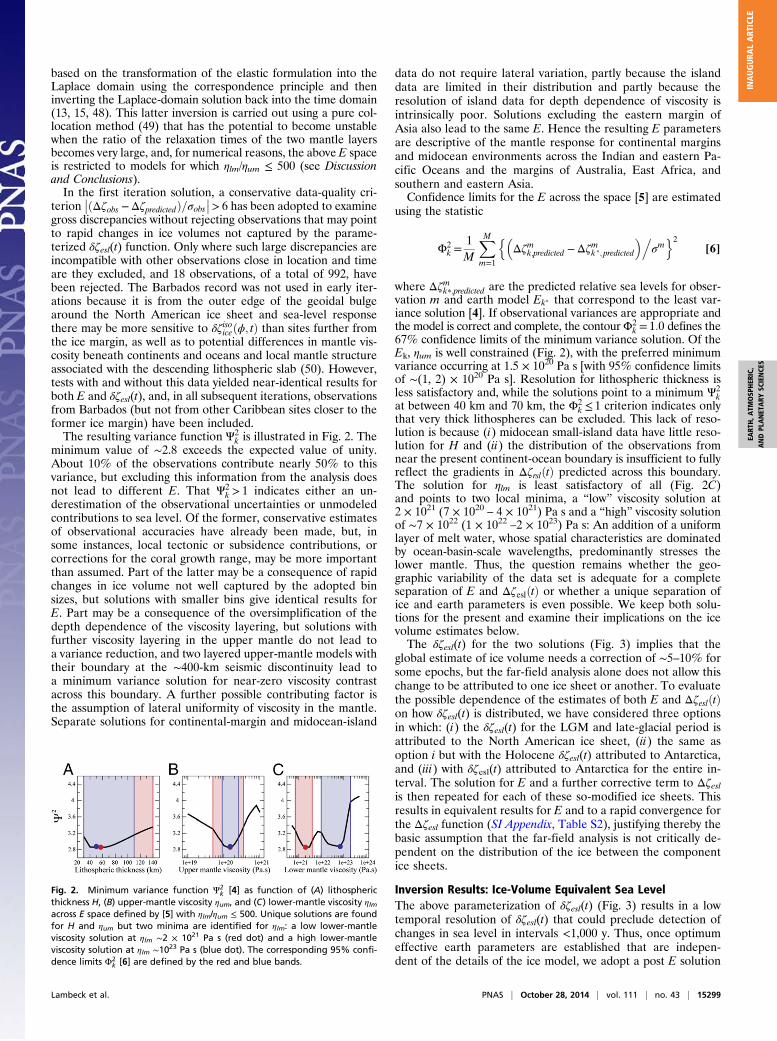
Fig. 2. Minimum variance function Ψ2k [4] as function of (A) lithospheric

thickness H, (B) upper-mantle viscosity ηum, and (C) lower-mantle viscosity ηlmacross E space defined by [5] with ηlm/ηum ≤ 500. Unique solutions are foundfor H and ηum but two minima are identified for ηlm: a low lower-mantleviscosity solution at ηlm ∼2 × 1021 Pa s (red dot) and a high lower-mantleviscosity solution at ηlm ∼1023 Pa s (blue dot). The corresponding 95% confi-dence limits Φ2

k [6] are defined by the red and blue bands.

Lambeck et al. PNAS | October 28, 2014 | vol. 111 | no. 43 | 15299

EART

H,A

TMOSP

HER

IC,

ANDPL

ANET

ARY

SCIENCE

SINAUGURA

LART

ICLE

processing approach to solve for the incremental δζesl(t) in whicheach observation Δζmobsðϕ; tÞ provides an estimate of esl

ΔζmeslðtÞ=Δζmobsðϕ; tÞ−hΔζmk p; predictedðϕ; tÞ−Δζ0eslðtÞ

i[7a]

with

�σmesl

�2 = �σmobsðϕ; tÞ

�2 + �σmk p; predictedðtÞ

�2: [7b]

The variance ðσmkp;predictedðtÞÞ2 follows from the variance of thepredicted values across the E space defined by the Φ2

k ≤ 1according to

σmk p; predicted

�2=

"Xk

Δζmk p; predicted −Δζmk; predicted

�2.σ2k

#,Xk

1�σ2k

[8]

with

σ2k =��1−Φ2

k

��2:

The underlying signal in the resulting noisy time series is thenestimated using the transdimensional Markov chain Monte Carloapproach (51) that allows abrupt or rapid changes to be quanti-fied against a background of long-term trends and that infers theprobability distributions on the number and location of changepoints, as well as the trends between change points. This produ-ces an ensemble of candidate time series curves, the collectivedensity of which follows a Bayesian a posteriori probability den-sity function (PDF) defined by the product of a likelihood anda priori PDF on control parameters. The algorithm avoids theneed to impose artificial constraints on model complexity byusing a flexible parameterization of the time series with a variablenumber of unknowns but at the same time remains parsimoniousin that it eliminates unwarranted detail in the reconstructed sig-nal. The mean of the ensemble is taken as an objective estimateof the underlying “denoised” time series while uncertainty esti-mates are obtained through appropriate projections of the en-semble. Uncertainty estimates, in terms of probability densityfunctions, are obtained for the entire time signal as well as loca-tion of the change points representing abrupt changes in gradient(SI Appendix, Text S2 and Fig. S1).Fig. 4 illustrates the result corresponding to the high-viscosity

lower mantle model, and that for the low-viscosity lower mantleis given in SI Appendix, Fig. S2. Solution with and without theChina data yield indistinguishable results, and the introductionof this generally lower-quality material has not distorted the

inferences that can be drawn about rates of global sea-levelchange but, rather, reinforces them.

Discussion and ConclusionsOn time scales of 105 years and less, sea-level change at tec-tonically stable regions is primarily a function of changing icevolumes and the Earth’s response to the changing ice-water load,but neither the ice history nor the response function is in-dependently known with the requisite precision for developingpredictive models. Observations of sea level through time doprovide constraints on the ice and rheology functions, but acomplete separation of the two groups of parameters has not yetbeen achieved. Separation of the analysis into far-field and near-field areas provides some resolution, but ambiguities remain:a consequence of inadequate a priori information on ice marginevolution and ice thickness, observational data that deterioratesin distribution and accuracy back in time, the likelihood of lateralvariations in the planet’s rheological response, and the ever-present possibility of tectonic contributions.We have focused here on the far-field analysis of nearly 1,000

observations of relative sea level for the past 35 ka, underpinnedby independent near-field analyses for the individual major icesheets of the Northern Hemisphere and inferences about thepast Antarctic ice sheet. Within the confines of model assump-tions and with one caveat, a separation can be achieved of ef-fective rheology parameters for the mantle beneath the oceansand continental margins and the change in total ice volume orice-volume esl. The caveat is that two solutions are possible,characterized as high-viscosity and low-viscosity lower-mantlemodels, each with its own esl function (SI Appendix, Fig. S2).One approach to separate earth and ice parameters could be tosearch for “dip-stick” sites (52) where the glacioisostatic andhydroisostatic components cancel and Δζrslðϕ; tÞ=Δζeslðϕ; tÞ.However, such contours do exhibit time and E dependence, andthere are few observations that actually lie close to the Δζiso = 0contour at any epoch (SI Appendix, Fig. S3).The esl obtained for the two solutions (Fig. 4 and SI Appendix,

Fig. S2) differ in two important respects: (i) at the LGM, thelow-viscosity model requires ∼2.7 × 106 km3 (∼7 m esl) more iceat the maximum glaciation than the high-viscosity model, and (ii)during the mid to late Holocene (the past ∼7 ka), the low-vis-cosity model requires less ice (∼0.5 × 106 km3 or ∼1.3 m esl at6 ka BP) than the high-viscosity model (the relaxation in the low-viscosity model is more complete than for a high-viscositymodel). Of these, the first difference may provide some guide tothe choice of solution.The changes in Antarctic ice volume since the LGM remain

poorly known, and published estimates differ greatly: ∼25–35 mof esl from the difference in far-field and Northern Hemispherenear-field estimates of changes in ice volume (53), ∼20 m fromthe combination of such methods with the inversion of rebounddata from the Antarctic margin (54), ∼10–18 m from glaciolog-ical models (55, 56), and ∼10 m from combined glaciological andgeological modeling (57). In developing our component icesheets, we have used an iterative approach in which, at any step,the Antarctic ice-volume function is the difference between thefar-field derived global estimate and the sum of the NorthernHemisphere and mountain glacier ice volumes for that iteration.This “missing” ice is then distributed within the ice sheet to re-spect the LGM Antarctic margin (58) and with the assumptionthat ice elevation profiles across the shelf and into the interiorapproximate a quasi-parabolic form (59). Thus, the intent of thisice sheet is only to preserve the global ocean−ice mass balanceand not to produce a realistic rebound model for far-southernlatitudes. The starting iteration of the present far-field solutionhas an Antarctic contribution to esl of 28 m (equivalent to ∼107 km3

of ice, with a large fraction of this ice grounded on the shelves; seeEq. 1). For the high-viscosity solution this is reduced to ∼23 m

Fig. 3. Low-definition solutions (1,000-y time bins) for the corrective term δζeslðtÞfor the two lower-mantle viscosity solutions (low-viscosity solution in red withyellow error bars and high-viscosity solution in blue with pale blue error bars).

15300 | www.pnas.org/cgi/doi/10.1073/pnas.1411762111 Lambeck et al.

whereas it is increased to ∼30 m for the low-viscosity solution. Thechoice of model could then be made on the basis of how much icecan plausibly be stored in Antarctica during the LGM, consistentwith other geological and glaciological constraints. On the basis ofthe comparison with independent estimates (55–57), we favor thehigh-viscosity model.Both solutions point to an ongoing slow increase in ocean

volume after 7 ka BP, even though melting of the large NorthernHemisphere ice sheets had largely ceased by this time. The highnorthern latitude Holocene Climate Optimum peaked between6 and 4 ka BP, and some Greenland ice-margin retreat occurredat least locally (60, 61). There is also evidence that some Antarcticmelting occurred after ∼6 ka BP (62). Furthermore, high andmidlatitude mountain glaciers, including remnants of LatePleistocene arctic and subarctic ice caps, may also have contin-ued to decrease in volume (63). However, in all cases, there isnot enough observational evidence to independently constrainglobal estimates of ice-mass fluctuations during this post-7-kaperiod to permit discrimination between the two esl solutions.One option is to impose constraints on the lower-mantle vis-

cosity from sources independent of the far-field results. Ouranalyses of rebound data from formerly glaciated regions (64)and of deglaciation-induced changes in the dynamic flatteningand rotation of the Earth (65–67) are consistent with the high-viscosity results, although these solutions are also ice-modeldependent. Inversions of geoid and seismic tomographic data areless sensitive to the choice of ice models (the observed geoidneeds corrections for the GIA contribution) and point to anincrease in depth-averaged mantle viscosity of one to threeorders of magnitude from average upper to lower mantle (68–73). Likewise, inferences of viscosity from the sinking speed ofsubducted lithosphere also point to high (3–5) × 1022 Pa s valuesfor the lower-mantle viscosity (74). On this basis, and because ityields the smaller volume for the LGM Antarctic ice volume, weadopt the high-viscosity lower-mantle solution.The adopted esl function illustrated in Fig. 4 and SI Appendix,

Table S3, shows many features previously identified in one ormore individual records but which, because it is based on geo-graphically well-spaced observations corrected for the isostatic

contributions, will reflect more accurately the changes in globallyaveraged sea level and ice volume. These features are:

i) A period of a relatively slow fall in sea level from 35 to31 ka BP followed by a rapid fall during 31–29 ka. Thisis based on data from Barbados, Bonaparte Gulf, HuonPeninsula (Papua New Guinea), and a few isolated obser-vations from the Malay Peninsula and the Bengal Fan. Itpoints to a period of rapid ice growth of ∼25 m esl within∼1,000 y to mark the onset of the peak glaciation, consis-tent with the transition out of the Scandinavian ÅlesundInterstadial into the glacial maximum (75), although thisice sheet alone is inadequate to contribute 25 m to esl.Chronologically, the timing of the rapid fall correspondsto the nominal age for the Heinrich H3 event (76, 77).

ii) Approximately constant or slowly increasing ice volumesfrom ∼29–21 ka BP. The data for this interval are sparsebut are from geographically well-distributed sites (Barbados,Bonaparte, Bengal Fan, East China Sea, and Maldives). Theslow increase in ice volume is consistent with eastward andsouthward expansion of the Scandinavian ice sheet duringthe LGM (78) as well as with the southward advance of theLaurentide ice sheet (79). The esl reaches its lowest value of∼134 m at the end of this interval, corresponding to ∼52 ×106 km3 more grounded ice—including on shelves—at theLGM than today. This is greater than the frequently cited−125 m (e.g., 24, 80) that is usually based on observationsuncorrected for isostatic effects. Heinrich event H2 at∼19.5–22 14C ka (∼25 ka BP) (77, 81, 82) is not associatedwith a recognizable sea-level signal.

iii) Onset of deglaciation at ∼21–20 ka BP with a short-livedglobal sea-level rise of ∼10–15 m before 18 ka. The evi-dence comes from the Bonaparte Gulf (37, 38), has beenidentified elsewhere (83, 84), and is supported by isolatedobservations from five other locations (Bengal Bay, Cape StFrancis (South Africa), offshore Sydney, Barbados, Mal-dives) which, although less precise than the principal dataset, spread the rise over a longer time interval than origi-nally suggested. Chronologically, this rise occurs substan-tially later than the H2 event.

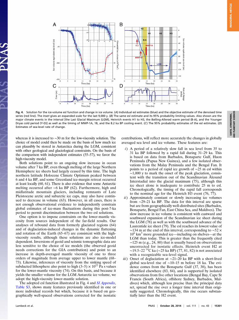
Fig. 4. Solution for the ice-volume esl function and change in ice volume. (A) Individual esl estimates (blue) and the objective estimate of the denoised timeseries (red line). The Inset gives an expanded scale for the last 9,000 y. (B) The same esl estimate and its 95% probability limiting values. Also shown are themajor climate events in the interval [the Last Glacial Maximum (LGM), Heinrich events H1 to H3, the Bølling-Allerød warm period (B-A), and the YoungerDryas cold period (Y-D)] as well as the timing of MWP-1A, 1B, and the 8.2 ka BP cooling event. (C) The 95% probability estimates of the esl estimates. (D)Estimates of sea-level rate of change.

Lambeck et al. PNAS | October 28, 2014 | vol. 111 | no. 43 | 15301

EART

H,A

TMOSP

HER

IC,

ANDPL

ANET

ARY

SCIENCE

SINAUGURA

LART

ICLE

iv) A short period of near-constant sea level from ∼18–16.5 kaBP. Support for this comes from observations fromBarbados, the Sunda Shelf, Bonaparte Gulf, Mayotte,and Cape St Francis.

v) A major phase of deglaciation from ∼16.5–7 ka BP. Thetotal esl change in this interval is ∼120 m, at an average rateof ∼12 m·ka−1, corresponding to a reduction of groundedice volume of ∼45 × 106 km3). Within this interval, signif-icant departures from the average occur.

vi) A rise of ∼25 m from ∼16.5–15 ka BP at the long-termaverage rate of ∼12 m·ka−1. The data are from Sunda,Tahiti, the East China Sea, Mayotte, and Australia. Chro-nologically, the onset of this rise occurs at the time of theH1 event dated at 16.8 ka (85) or 16 ka (86). This period ofrising sea level is followed by a short period (∼500–600 y) ofnear-constant sea level.

vii) A high rate of sea-level rise starting at ∼14.5 ka BP of ∼500 yduration. The onset occurs at the start of the Bølling−Allerød warm period. Its duration could be <500 y becauseof uncertainties in chronology, and the globally averaged risein sea level of ∼20 m occurs at a rate of ∼40 mm·y−1 orgreater. This pulse, MWP-1A, has been identified separatelyin the records of Barbados (24), Sunda (33), and Tahiti (28,87). Spatial variation in its amplitude can be expected be-cause of the planet’s elastic and gravitational response torapid unloading of ice in either or both of the two hemi-spheres (88) with, based on the ice−earth models used here,model-predicted values ranging from ∼14 m for Barbados to∼20 m for Tahiti (SI Appendix, Fig. S4). This compares withobservational values of ∼15–20 m (24, 28) for Barbados and12–22 m for Tahiti (28). Observational uncertainties remainlarge, including differences in the timing of this event asrecorded at the different localities, and it is not possible fromthis evidence to ascertain the relative importance of the con-tribution of the two hemispheres to MWP-1A.

viii) A period of sea-level rise from ∼14 to ∼12.5 ka BP of∼20 m in 1,500 y. The rate of rise is near the long-termaverage. Data are relatively dense in this interval and comefrom well-distributed sites (Barbados, Tahiti, Sunda, HuonPeninsula, Australia and New Zealand, Indian Ocean, andthe Yellow and East China seas).

ix) A period of a much reduced rate of rise from ∼12.5–11.5 kaBP. This short duration pause in the sea-level rise has beentenuously noted before in both composite (89) and individual(27) records. The chronology corresponds to the timing of theYounger Dryas stadial of the Northern Hemisphere whenretreat of the Northern Hemisphere ice sheets ceased mo-mentarily.

x) A period from ∼11.4–8.2 ka BP of near-uniform global rise.The average rate of rise during this 3.3 ka interval was∼15 m·ka−1 with little convincing evidence of variationsin this rate. A rapid rise, MWP-1B, has been reported at∼11.3 ka but remains elusive (27) and is not seen in thecomposite record other than as a slightly higher rate ofincrease to ∼16.5 mm·y−1 for a 500-y period immediatelyafter the Younger Dryas period.

xi) A reduced rate of sea-level rise for 8.2–6.7 ka BP. This isconsistent with the final phase of North American deglacia-tion at ∼7 ka BP. A marked cooling event has been recordedat 8.2 ka BP in Greenland and North Atlantic cores (90), butthere is no suggestion in the sea-level record of a corre-sponding fall or slowdown in global sea-level rise. Thedetailed local record from Singapore from 8.5 to 6 kaBP (40, 41) is consistent with the global rates within thisinterval except that a period of near-zero rise from 7.8 to7.4 ka is not seen globally, possibly lost in the noise ofother observations at around this time, possibly because itreflects local phenomena (Fig. 4).

xii) A progressive decrease in rate of rise from 6.7 ka to recenttime. This interval comprises nearly 60% of the database(Fig. 1). The total global rise for the past 6.7 ka was ∼4 m(∼1.2 × 106 km3 of grounded ice), of which ∼3 m occurredin the interval 6.7–4.2 ka BP with a further rise of ≤1 m upto the time of onset of recent sea-level rise ∼100–150 y ago(91, 92). In this interval of 4.2 ka to ∼0.15 ka, there is noevidence for oscillations in global-mean sea level of ampli-tudes exceeding 15–20 cm on time scales of ∼200 y (aboutequal to the accuracy of radiocarbon ages for this period,taking into consideration reservoir uncertainties; also, binsof 200 y contain an average of ∼15 observations/bin). Thisabsence of oscillations in sea level for this period is consis-tent with the most complete record of microatoll data fromKiritimati (23). The record for the past 1,000 y is sparsecompared with that from 1 to 6.7 ka BP, but there is noevidence in this data set to indicate that regional climatefluctuations, such as the Medieval warm period followed bythe Little Ice Age, are associated with significant globalsea-level oscillations.

ACKNOWLEDGMENTS. In addition to the support from our home institu-tions, this research has been partially funded by the Chaires Internationalesde Recherche Blaise Pascal de l’État Français et la Région Île de France, theInternational Balzan Foundation, and the Australian Research Council. Thedevelopment of the Baysian partition modeling software was partly sup-ported by the Auscope Inversion Laboratory, funded by the AustralianFederal Government.

1. Lambeck K, Chappell J (2001) Sea level change through the last glacial cycle. Science

292(5517):679–686.2. Chappell J, Shackleton NJ (1986) Oxygen isotopes and sea level. Nature 324:137–140.3. Waelbroeck C, et al. (2002) Sea-level and deep water temperature changes derived

from benthic foraminifera isotopic records. Quat Sci Rev 21:295–305.4. Ferranti L, et al. (2006) Markers of the last interglacial sea-level high stand along the

coast of Italy: Tectonic implications. Quat Int 145-146:30–54.5. Davies PJ, Marshall JF, Hopley D (1985) Relationships between reef growth and sea

level in the Great Barrier Reef. Proceedings of the Fifth International Coral Reef

Congress (Ecole Pratique des Hautes Etudes, Paris), Vol 5, pp 95–103.6. Lambeck K, et al. (2011) Sea level and shoreline reconstructions for the Red Sea:

Isostatic and tectonic considerations and implications for hominin migration out of

Africa. Quat Sci Rev 30:3542–3574.7. Shackleton NJ (1987) Oxygen isotopes, ice volume and sea level. Quat Sci Rev 6:

183–190.8. Lisiecki LE, Raymo ME (2005) A Pliocene-Pleistocene stack of 57 globally distributed

benthic δ18O records. Paleoceanography 20(1):PA1003.9. Shackleton NJ, Imbrie J, Hall MA (1983) Oxygen and carbon isotope record of East

Pacific core V19-30: Implications for the formation of deep water in the late Pleis-

tocene North Atlantic. Earth Planet Sci Lett 65:233–244.10. Rohling EJ, et al. (2009) Antarctic temperature and global sea level closely coupled

over the past five glacial cycles. Nat Geosci 2:500–504.

11. Moucha R, et al. (2008) Dynamic topography and long-term sea-level variations: Thereis no such thing as a stable continental platform. Earth Planet Sci Lett 271:101–108.

12. McKay NP, Overpeck JT, Otto-Bliesner BL (2011) The role of ocean thermal expansionin Last Interglacial sea level rise. Geophys Res Lett 38(14):L14605.

13. Cathles LM (1975) The Viscosity of the Earth’s Mantle (Princeton Univ Press, Princeton, NJ).14. Peltier WR, Andrews JT (1976) Glacial-isostatic adjustment-I. The forward problem.

Geophys J R Astron Soc 46:605–646.15. Nakada M, Lambeck K (1987) Glacial rebound and relative sea-level variations: A new

appraisal. Geophys J R Astron Soc 90:171–224.16. Mitrovica JX, Milne GA (2002) On the origin of late Holocene sea-level highstands

within equatorial ocean basins. Quat Sci Rev 21:2179–2190.17. Mitrovica JX, Wahr J (2011) Ice Age Earth rotation. Annu Rev Earth Planet Sci 39:

577–616.18. Farrell WE, Clark JA (1976) On postglacial sea level. Geophys J R Astron Soc 46:

647–667.19. Reimer PJ, et al. (2009) IntCal09 and Marine09 radiocarbon age calibration curves,

0−50,000 years cal BP. Radiocarbon 51:1111–1150.20. Montaggioni LF (2009) Quaternary Coral Reef Systems: History, Development Pro-

cesses and Controlling Factors, ed Braithwaite CJR (Elsevier, Amsterdam).21. Woodroffe C, McLean R (1990) Microatolls and recent sea level change on coral atolls.

Nature 344:531–534.22. Chappell J (1983) Evidence for smoothly falling sea level relative to north Queensland,

Australia, during the past 6,000 yr. Nature 302:406–408.

15302 | www.pnas.org/cgi/doi/10.1073/pnas.1411762111 Lambeck et al.

23. Woodroffe CD, McGregor HV, Lambeck K, Smithers SG, Fink D (2012) Mid-Pacificmicroatolls record sea-level stability over the past 5000 yr. Geology 40:951–954.

24. Fairbanks RG (1989) A 17,000-year glacio-eustatic sea level record: Influence of glacialmelting rates on the Younger Dryas event and deep-ocean circulation. Nature 342:637–642.

25. Bard E, Hamelin B, Fairbanks RG (1990) U-Th ages obtained by mass spectrometry incorals from Barbados: Sea level during the past 130,000 years. Nature 346:456–458.

26. Peltier WR, Fairbanks RG (2006) Global glacial ice volume and Last Glacial Maximumduration from an extended Barbados sea level record. Quat Sci Rev 25:3322–3337.

27. Bard E, Hamelin B, Delanghe-Sabatier D (2010) Deglacial meltwater pulse 1B andYounger Dryas sea levels revisited with boreholes at Tahiti. Science 327(5970):1235–1237.

28. Deschamps P, et al. (2012) Ice-sheet collapse and sea-level rise at the Bølling warming14,600 years ago. Nature 483(7391):559–564.

29. Chappell J, Polach H (1991) Post-glacial sea-level rise from a coral record at HuonPeninsula, Papua New Guinea. Nature 349:147–149.

30. Yokoyama Y, Esat TM, Lambeck K (2001) Coupled climate and sea-level changesdeduced from Huon Peninsula coral terraces of the last ice age. Earth Planet Sci Lett193:579–587.

31. Camoin GF, Montaggioni LF, Braithwaite CJR (2004) Late glacial to post glacial sealevels in the Western Indian Ocean. Mar Geol 206:119–146.

32. Van de Plassche O, ed. (1986) Sea-Level Research: A Manual for the Collection andEvaluation of Data (Geo Books, Norwich, UK).

33. Hanebuth T, Stattegger K, Grootes PM (2000) Rapid flooding of the Sunda Shelf: Alate-glacial sea-level record. Science 288(5468):1033–1035.

34. Hanebuth TJJ, Stattegger K, Bojanowski A (2009) Termination of the Last GlacialMaximum sea-level lowstand: The Sunda-Shelf data revisited. Global Planet Change66:76–84.

35. Zinke J, et al. (2003) Postglacial flooding history of Mayotte Lagoon (Comoro Archi-pelago, southwest Indian Ocean). Mar Geol 194:181–196.

36. Wiedicke M, Kudrass H-R, Hübscher C (1999) Oolitic beach barriers of the last Glacialsea-level lowstand at the outer Bengal shelf. Mar Geol 157:7–18.

37. Yokoyama Y, Lambeck K, Johnston P, Fifield LK, Fifield L, De Deckker P (2000) Timingof the Last Glacial Maximum from observed sea-level minima. Nature 406(6797):713–716.

38. De Deckker P, Yokoyama Y (2009) Micropalaeontological evidence for Late Quater-nary sea-level changes in Bonaparte Gulf, Australia. Global Planet Change 66:85–92.

39. Gibb JG (1986) A New Zealand regional Holocene eustatic sea level curve and itsapplication for determination of vertical tectonic movements. Bull R Soc N Z 24:377–395.

40. Bird MI, et al. (2007) An inflection in the rate of early mid-Holocene eustatic sea-levelrise: A new sea-level curve from Singapore. Estuarine Coastal Shelf Sci 71:523–536.

41. Bird MI, et al. (2010) Punctuated eustatic sea-level rise in the early mid-Holocene.Geology 38:803–806.

42. Geyh MA, Kudrass H-R, Streif H (1979) Sea-level changes during the Late Pleistoceneand Holocene in the Straits of Malacca. Nature 278:441–443.

43. Dutton A, Lambeck K (2012) Ice volume and sea level during the last interglacial.Science 337(6091):216–219.

44. Kopp RE, Simons FJ, Mitrovica JX, Maloof AC, Oppenheimer M (2013) A probabilisticassessment of sea level variations within the last interglacial stage. Geophys J Int 193:711–716.

45. Xie X, Müller RD, Li S, Gong Z, Steinberger B (2006) Origin of anomalous subsidencealong the northern South China Sea margin and its relationship to dynamic topog-raphy. Mar Pet Geol 23:745–765.

46. Lambeck K, Smither C, Johnston P (1998) Sea-level change, glacial rebound andmantle viscosity for northern Europe. Geophys J Int 134:102–144.

47. Paulson A, Zhong S, Wahr J (2007) Limitations on the inversion for mantle viscosityfrom postglacial rebound. Geophys J Int 168:1195–1209.

48. Peltier WR (1974) The impulse response of a Maxwell Earth. Rev Geophys Space Phys12:649–669.

49. Mitrovica JX, Peltier WR (1992) A comparison of methods for the inversion of visco-elastic relaxation spectra. Geophys J Int 108:410–414.

50. Austermann J, Mitrovica JX, Latychev K, Milne A (2013) Barbados-based estimateof ice volume at Last Glacial Maximum affected by subducted plate. Nat Geosci6:553–557.

51. Gallagher K, et al. (2011) Inference of abrupt changes in noisy geochemical recordsusing transdimensional changepoint models. Earth Planet Sci Lett 311:182–194.

52. Milne GA, Mitrovica J (2008) Searching for eustasy in deglacial sea-level histories.Quat Sci Rev 27:2292–2302.

53. Nakada M, Lambeck K (1988) Late Pleistocene and Holocene sea-level: Implicationsfor mantle rheology and the melting history of the Antarctic ice sheet. J Seis Soc Jap41:443–455.

54. Nakada M, et al. (2000) Late Pleistocene and Holocene melting history of theAntarctic ice sheet derived from sea-level variations. Mar Geol 167:85–103.

55. Philippon G, et al. (2006) Evolution of the Antarctic ice sheet throughout the lastdeglaciation: A study with a new coupled climate—north and south hemisphere icesheet model. Earth Planet Sci Lett 248:750–758.

56. Pollard D, DeConto RM (2009) Modelling West Antarctic ice sheet growth and col-lapse through the past five million years. Nature 458(7236):329–332.

57. Whitehouse PL, Bentley MJ, Le Brocq AM (2012) A deglacial model for Antarctica:Geological constraints and glaciological modelling as a basis for a new model ofAntarctic glacial isostatic adjustment. Quat Sci Rev 32:1–24.

58. Anderson JB, Shipp SS, Lowe AL, Wellner JS, Mosola AB (2002) The Antarctic ice sheetduring the Last Glacial Maximum and its subsequent retreat history: A review. QuatSci Rev 21:49–70.

59. Cuffey K, Paterson WSB (2010) The Physics of Glaciers (Elsevier, Amsterdam).60. Weidick A, Oerter H, Reeh N, Thomsen HH, Thorning L (1990) The recession of the

inland ice margin during the Holocene climatic optimum in the Jakobshavn Isfjordarea of West Greenland. Global Planet Change 2:389–399.

61. Briner JP, Håkansson L, Bennike O (2013) The deglaciation and neoglaciation ofUpernavik Isstrøm, Greenland. Quat Res 80:459–467.

62. Stone JO, et al. (2003) Holocene deglaciation of Marie Byrd Land, West Antarctica.Science 299(5603):99–102.

63. Denton GH (1981) The Last Great Ice Sheets, ed Hughes TJ (Wiley, New York).64. Lambeck K, Purcell A, Zhao J, Svensson N-O (2010) The Scandinavian Ice Sheet: From

MIS 4 to the end of the Last Glacial Maximum. Boreas 39:410–435.65. O’Connell RJ (1971) Pleistocene glaciation and the viscosity of the lower mantle.

Geophys J Int 23:299–327.66. Johnston P, Lambeck K (1999) Postglacial rebound and sea level contributions to

changes in the geoid and the Earth’s rotation axis. Geophys J Int 136:537–558.67. Kaufmann G, Lambeck K (2002) Glacial isostatic adjustment and the radial viscosity

profile from inverse modeling. J Geophys Res 107(B11):2280.68. Hager BH, Richards MA (1989) Long-wavelength variations in Earth’s geoid: Physical

models and dynamical implications. Philos Trans R Soc A Math Phys. Eng Sci 328:309–327.

69. Ricard Y, Wuming B (1991) Inferring the viscosity and the 3-D density structure of themantle from geoid, topography and plate velocities. Geophys J Int 105:561–571.

70. King SD, Masters G (1992) An inversion for radial viscosity structure using seismictomography. Geophys Res Lett 19:1551–1554.

71. �Cadek O, Fleitout L (1999) A global geoid model with imposed plate velocities andpartial layering. J Geophys Res 104(B12):29055−29075.

72. Mitrovica JX, Forte AM (2004) A new inference of mantle viscosity based upon jointinversion of convection and glacial isostatic adjustment data. Earth Planet Sci Lett225:177–189.

73. Steinberger B, Calderwood AR (2006) Models of large-scale viscous flow in the Earth’smantle with constraints from mineral physics and surface observations. Geophys J Int167:1461–1481.

74. �Cí�zková H, van den Berg AP, Spakman W, Matyska C (2012) The viscosity of Earth’slower mantle inferred from sinking speed of subducted lithosphere. Phys Earth PlanetInter 200-201:56–62.

75. Mangerud J, Gyllencreutz R, Lohne Ø, Svendsen JI (2011) Glacial history of Norway.Quaternary Glaciations - Extent and Chronology: A Closer Look, eds Ehlers J,Gibbard PL, Hughes PD (Elsevier, Amsterdam), pp 279–298.

76. Bond GC, Lotti R (1995) Iceberg discharges into the North Atlantic on millennial timescales during the last glaciation. Science 267(5200):1005–1010.

77. Marcott SA, et al. (2011) Ice-shelf collapse from subsurface warming as a trigger forHeinrich events. Proc Natl Acad Sci USA 108(33):13415–13419.

78. Boulton GS, Dongelmans P, Punkari M, Broadgate M (2001) Palaeoglaciology of an icesheet through a glacial cycle: The European ice sheet through the Weichselian. QuatSci Rev 20:591–625.

79. Dyke AS, et al. (2002) The Laurentide and Innuitian ice sheets during the Last GlacialMaximum. Quat Sci Rev 21:9–31.

80. Siddall M, et al. (2003) Sea-level fluctuations during the last glacial cycle. Nature423(6942):853–858.

81. Vidal L, et al. (1999) Link between the North and South Atlantic during the Heinrichevents of the last glacial period. Clim Dyn 15:909–919.

82. Grousset F, Pujol C, Labeyrie L, Auffret G, Boelaert A (2000) Were the North AtlanticHeinrich events triggered by the behavior of the European ice sheets? Geology 28:123–126.

83. Clark PU, McCabe AM, Mix AC, Weaver AJ (2004) Rapid rise of sea level 19,000 yearsago and its global implications. Science 304(5674):1141–1144.

84. Carlson AE, Clark PU (2012) Ice sheet sources of sea level rise and freshwater dischargeduring the last deglaciation. Rev Geophys 50(4), RG4007.

85. Clark PU, et al. (2001) Freshwater forcing of abrupt climate change during the lastglaciation. Science 293(5528):283–287.

86. Hemming SR (2004) Heinrich events: Massive late Pleistocene detritus layers of theNorth Atlantic and their global climate imprint. Rev Geophys 42(1):RG1005.

87. Bard E, et al. (1996) Deglacial sea-level record from Tahiti corals and the timing ofglobal meltwater discharge. Nature 382:241–244.

88. Clark P, Mitrovica J, Milne G, Tamisiea M (2002) Sea-level fingerprinting as a directtest for the source of global meltwater pulse IA. Science 295:2438–2441.

89. Lambeck K, Yokoyama Y, Purcell A (2002) Into and out of the Last Glacial Maximumsea level change during oxygen isotope stages 3-2. Quat Sci Rev 21:343–360.

90. Alley RB, et al. (1997) Holocene climatic instability: A prominent, widespread event8200 yr ago. Geology 25:483–486.

91. Lambeck K, Anzidei M, Antonioli F, Benini A, Esposito A (2004) Sea level in Romantime in the Central Mediterranean and implications for recent change. Earth PlanetSci Lett 224:563–575.

92. Kemp AC, et al. (2009) Timing and magnitude of recent accelerated sea-level rise(North Carolina, United States). Geology 37:1035–1038.

Lambeck et al. PNAS | October 28, 2014 | vol. 111 | no. 43 | 15303

EART

H,A

TMOSP

HER

IC,

ANDPL

ANET

ARY

SCIENCE

SINAUGURA

LART

ICLE