Embed Size (px)
Citation preview
Forthcoming in the American Economic Journal: Applied Economics
School Inputs, Household Substitution, and Test Scores
Jishnu Das Stefan Dercon James Habyarimana Pramila Krishnan Karthik Muralidharan Venkatesh Sundararaman*
22 May 2012*
Abstract: Empirical studies of the relationship between school inputs and test scores typically do not account for household responses to changes in school inputs. Evidence from India and Zambia shows that student test scores are higher when schools receive unanticipated grants; but there is no impact of grants that are anticipated. We show that the most likely mechanism for this result is that households offset their own spending in response to anticipated grants. Our results confirm the importance of optimal household responses and suggest caution when interpreting estimates of school inputs on learning outcomes as parameters of an education production function. JEL Classification: H52, I21, O15
Keywords: school grants, school inputs, household substitution, education in developing countries, randomized experiment, India, Zambia, Africa, education production function
*Das: The World Bank, MSN MC3-311, 1818 H Street, NW Washington, DC 20433 (email:[email protected]); Dercon: Oxford University, Department of International Development, 3 Mansfield Road, Oxford OX1 3TB, United Kingdom (email: [email protected] ); Habyarimana: Georgetown Public Policy Institute, 37th & O street NW, Old North, Room 307, Washington DC 20057 (email: [email protected] ); Krishnan: University of Cambridge, Faculty of Economics, Austin Robinson Building, Sidgewick Avenue, Cambridge CB3 9DD, UK (email: [email protected]); Muralidharan: University of California, San Diego, Department of Economics, 9500 Gilman Drive #0508, La Jolla, CA 92093-0508 (email: [email protected]); Sundararaman: The World Bank, Yak and Yeti Hotel Complex, Durbar Marg, Kathmandu, Nepal (email: [email protected]). We thank Julie Cullen, Gordon Dahl, Roger Gordon, Gordon Hanson, Hanan Jacoby, Andres Santos, and several seminar participants for comments. The World Bank and the UK Department for International Development (DFID) provided financial support for both the Zambia and India components of this paper. The experiment in India is part of a larger project known as the Andhra Pradesh Randomized Evaluation Study (AP RESt), which is a partnership between the Government of Andhra Pradesh, the Azim Premji Foundation, and the World Bank. We thank Dileep Ranjekar, Amit Dar, Samuel C. Carlson, and officials of the Department of School Education in Andhra Pradesh for their continuous support. We are especially grateful to DD Karopady, M Srinivasa Rao, and staff of the Azim Premji Foundation for their leadership in implementing the project in Andhra Pradesh. Vinayak Alladi, Jayash Paudel, and Ketki Sheth provided excellent research assistance. The findings, interpretations, and conclusions expressed in this paper are those of the authors and do not necessarily represent the views of the Government of Andhra Pradesh, the Azim Premji Foundation, or the World Bank, its Executive Directors, or the governments they represent.
1
The relationship between school inputs and education outcomes is of fundamental
importance for education policy and has been the subject of hundreds of empirical studies around
the world (see Hanushek 2002, and Hanushek and Luque 2003 for reviews of US and
international evidence respectively). However, while the empirical public finance literature has
traditionally paid careful attention to the behavioral responses of agents to public programs1, the
empirical literature estimating education production functions has typically not accounted for
household re-optimization in response to public spending.2 To the extent that such behavioral
responses are large, they will (a) mediate the extent to which different types of education
spending translate into improvements in learning, and (b) limit our ability to identify parameters
of an education production function.
Using a simple household optimization framework, we clarify how increases in school inputs
may affect household spending responses and, in turn, learning outcomes. In this framework,
households' optimal spending decisions take into account all information available at the time of
decision making. The impact of school inputs on test scores depends then on (a) whether such
inputs are anticipated or not and (b) the extent of substitutability between household and school
inputs in the education production function. The model predicts that if household and school
inputs are technical substitutes, an anticipated increase in school inputs in the next period will
decrease household contributions that period. Unanticipated increases in school inputs limit the
scope for household responses, leaving household contributions unchanged in the short run.
These differences lead to a testable prediction: If household and school inputs are (technical)
substitutes, unanticipated inputs will have a larger impact on test scores than anticipated inputs.
We examine the implications of the model in India and Zambia using panel data on student
achievement combined with unique matched data sets of school and household spending. We
measure changes in household spending as well as student test-score gains in response to both
unanticipated as well as anticipated changes in school funding, and highlight the empirical
salience of this difference. The former is more likely to capture the production function effect of
1Illustrative examples include Meyer (1990) on unemployment insurance, Cutler and Gruber (1996) on health insurance, Eissa and Leibman (1996) on the EITC, Autor and Duggan (2003) on disability insurance. See Moffitt (2002) for an overview on labor supply responses to welfare programs. 2 An exception is the study of household responses to school feeding programs (see Powell et al. 1998 and Jacoby 2002). Evaluations of other educational interventions have recently started collecting data on changes in household inputs in response to the programs (see Glewwe et al. 2009 and Pop-Eleches and Urquiola 2011)
2
increased school funding (a partial derivative holding other inputs constant), while the latter
measures the policy effect (a total derivative that accounts for re-optimization by agents).
Our first set of results is based on experimental variation in school funds induced by a
randomly-assigned school grant program in the Indian state of Andhra Pradesh (AP). The AP
school block grant experiment was conducted across a representative sample of 200 government-
run schools in rural AP with 100 schools selected by lottery to receive a school grant (worth
around $3 per pupil) over and above their regular allocation of teacher and non-teacher inputs.
The conditions of the grant specified that the funds were to be spent on inputs used directly by
students and not on infrastructure or construction projects, and the majority of the grant was
typically spent on notebooks, writing materials, workbooks, and stationery – material that
households could also purchase on their own The program was implemented for two years. In
the first year, the grant (assigned by lottery) was a surprise for recipient schools that was
announced and provided around two months into the school year (whereas the majority of
household spending on materials typically takes place at the start of the school year). In the
second year the grant was anticipated by parents and teachers of program schools, and the
knowledge of the grant could potentially have been incorporated into decisions regarding
household spending on education.
Our strongest results are that household education spending in program schools does not
change in the first year (relative to spending in the control schools), but that it is significantly
lower in the second year suggesting that households offset the anticipated grant significantly
more than they offset the unanticipated grant. Evaluated at the mean, we find that for each dollar
provided to treatment schools in the second year, household spending declines by 0.76 dollars.
We cannot reject that the grant is completely offset by the household, while the lower bound of a
95% confidence interval suggests that at least half is crowded out. In short, we find considerable
crowding out of the school grant by households in the second year.
Consistent with this, we find that students in program schools perform significantly better
than those in comparison schools at the end of the first year of the school grant program, scoring
0.08 and 0.09 standard deviations more in language and mathematics tests respectively for a
transfer of a little under $3 per pupil. In the second year, the treatment effects of the program are
considerably lower and not significantly different from zero. These results suggest that the
3
production-function effect of the school grants on test scores was positive, but that the policy
effects are likely to be lower once households re-optimize their own spending.
The experimental study in AP is complemented with data from Zambia, which allow us to
examine a scaled up school grant program implemented across an entire country by a national
government. Starting in 2001, the Government of Zambia started providing all schools in the
country with a fixed block grant of $600-650 (regardless of enrollment) as part of a nationally
well-publicized program. Thus, variation in school enrollment led to substantial cross-sectional
variation in the per-student funding provided by this rule-based grant. We find, however, that
per-student variation in the block grant is not correlated with any differences in student test score
gains. As in AP, we collect data on household spending and find that household spending almost
completely offsets variations in predicted per-student school grants, suggesting that household
offset may have been an important channel for the lack of correlation between public education
spending and test score gains. We further exploit the presence of a discretionary district-level
source of funding that is highly variable across schools and much less predictable than the rule-
based grant and find that student test scores in schools receiving these funds are 0.10 standard
deviations higher for both the English and mathematics tests for a median transfer of just under
$3 per pupil.
These two sets of results complement each other and provide greater external validity to our
findings. The AP case offers experimental variation in one source of funding, which changes
from being unanticipated to anticipated over time. The Zambia case offers an analysis of two
contemporaneously different sources of funding (rule-based and discretionary) in a scaled up
government-implemented setting, but relies on non-experimental data.
There are important policy implications of our results. The impact of anticipated school
grants in both settings is low, not because the money did not reach the schools (it did) or because
it was not spent well (there is no evidence to support this), but because households realigned
their own spending patterns optimally across time and other spending, and not just on their
children’s education. The replication of the findings in two very different settings3, with two
3At the time of the study, Zambia experienced severe declines in per-capita government education expenditure and a stagnant labor market, while Andhra Pradesh has been one of the fastest growing states in India with large increases in government spending in education over the last decade. Our finding very similar results in a dynamic, growing economy and in another that was, at best, stagnant at the time of our study suggests that the results generalize across very different labor market conditions and the priority given to education in the government's budgetary framework.
4
different implementing agencies (a leading non-profit organization in AP, and the government in
Zambia), and in representative population-based samples suggests that the impact of school grant
programs is likely to be highly attenuated by household responses. This has direct implications
for thinking about the effectiveness of many such school grant programs across several
developing countries.4
The distinction between anticipated and unanticipated inputs and the differential ability of
households to substitute across various inputs may account for the wide variation in estimated
coefficients of school inputs on test scores (Glewwe 2002, Hanushek 2003, or Krueger 2003),
and our results highlight the empirical importance of distinguishing between policy effects and
production function parameters (see Todd and Wolpin 2003, Glewwe and Kremer 2005, Glewwe
et al. 2009, and Pop-Eleches and Urquiola 2011). A failure to reject the null hypothesis in studies
that use the production function approach could arise either because the effect of school inputs
on test scores through the production function is zero or because households (or teachers or
schools) substitute their own resources for such inputs.
While we are able to demonstrate substitution that takes the form of textbooks or writing
materials, such responses may have extended to changes in parental time, private tuition and
other inputs. For instance, Houtenville and Conway (2008) find that parental effort is negatively
correlated with school resources and, Liu, Mroz, and van der Klaauw (2010) show that maternal
labor force participation decisions respond to school quality. In their work on Kenya, Duflo,
Dupas and Kremer (2012) find evidence of reduced effort among existing teachers when schools
are provided with an extra contract teacher, a result that is also documented in an experimental
study of contract teachers in India (Muralidharan and Sundararaman 2012). Our results should
therefore be interpreted as offering evidence that changes in household expenditure are likely to
be an important explanation for the declining impact of the school grant on test scores between
the first and second year of the program, but we do not claim that it is the only reason for this
difference.
The remainder of the paper is structured as follows. Section 2 describes a simple framework
that motivates our estimating equations. Section 3 presents results from the experimentally-
4Examples include school grants under the Sarva Shiksha Abhiyan (SSA) program in India, the Bantuan Operasional Sekolah (BOS) grants in Indonesia, and several similar school grant programs in African countries (see Reinikka and Svensson 2004 for descriptions of school grant programs in Uganda, Tanzania, and Ghana).
5
assigned school grant experiment in India, and discusses robustness to alternative interpretations
and mechanisms. Section 4 presents results from a nationally scaled up school grant program in
Zambia. Section 5 concludes with remarks on policy and alternate experiments in this domain.
I. A Simple Framework
In a parallel working paper (Das et al 2011), we offer an analytical framework to organize
the empirical investigation and interpret the results. Building on Becker and Tomes (1976) and
Todd and Wolpin (2003), we examine the interaction of school and household inputs within the
context of optimizing households to derive empirical predictions. The model has two
components. First, households derive utility from the test-scores of a child, TS, and the
consumption of other goods. Households maximize an inter-temporal utility function subject to
an inter-temporal budget constraint. Second, test scores are determined by a production function
relating current achievement TSt to past achievement TSt-1, household educational inputs zt,
school inputs tw and non time-varying child and school characteristics.
In this framework, there are two reasons for why an unanticipated increase in school
resources will have a greater impact on student test score gains than an anticipated one. First,
when household and school inputs are technical substitutes, an anticipated increase in school
inputs allows households to re-allocate spending from education towards other commodities
(whereas unanticipated increases in school inputs provide less scope for such reallocation if these
resources arrive after the majority of education spending has already taken place at the beginning
of the school year). Second, when household and school inputs are technical substitutes, and the
production function is concave in these inputs, an increase in school inputs decreases the
marginal product of home inputs. Anticipated increases in school inputs thus increase the
relative cost of boosting TS, creating price incentives to shift resources from education to other
commodities.
An empirical specification consistent with the model is:
ituit
aito
it
it wwTS
TS
lnlnln 211
(1)
Here, aitw and u
itw are anticipated and unanticipated changes in school inputs, measured in this
paper by the flows of funds. The core prediction is that the marginal effect of anticipated funds
(α1) is lower than that of unanticipated funds (α2) when household and school inputs are
6
substitutes.5 Finally, if a portion of what the econometrician regards as unanticipated was
anticipated by the household (or was substitutable even after the 'surprise' arrival of the school
grant), then the estimate of α2 will be a lower bound of the true production function effect.
II. The AP School Block Grant Experiment
A. Background and Context
We examine these predictions within the context of an experimental intervention in Andhra
Pradesh (AP), the 5th largest state in India, with a population of over 80 million of which more
than 70% live in rural areas. AP is close to the all-India average on various measures of human
development such as gross enrollment in primary school, literacy, and infant mortality, as well as
on measures of service delivery such as teacher absence (Kremer et al. 2005). There are a total of
over 60,000 government primary schools in AP and over 70% of children in rural AP attend
government-run schools (Pratham 2010).
The average rural primary school is quite small, with total enrollment of around 80 to 100
students and an average of 3 teachers across grades one through five. Teachers are well paid,
with the average salary of regular civil-service teachers being over Rs. 8,000/month and total
compensation including benefits being over Rs. 10,000/month (per capita income in AP is
around Rs. 2,000/month). Regular teachers' salaries and benefits comprise over 90% of non-
capital expenditure on primary education in AP, leaving relatively little funds for recurring non-
teacher expenses.6
Some of these funds are used to provide schools with an annual grant of Rs. 2,000 for
discretionary expenditures on school improvement and to provide each teacher with an annual
grant of Rs. 500 for the purchase of classroom materials of the teachers’ choice. The
government also provides children with free text books through the school. However, compared
to the annual spending on teacher salaries of over Rs. 300,000 per primary school (three teachers
per school on average) the amount spent on learning materials is very small. It has been
5 With credit constraints, anticipated increases in school spending will alleviate the overall and period-specific budget constraint of the household resulting in greater current spending on all goods, including education. But the response in terms of overall educational spending will still be smaller than in the case of unanticipated increases, as the gain in the available budget will be re-allocated across all commodities in the households’ utility function, and not spent only on education (see Das et al 2011). 6 Funds for capital expenditure (school construction and maintenance) come from a different part of the budget. Note that all figures correspond to the years 2005 - 07, which is the time of the study, unless stated otherwise.
7
suggested therefore that the marginal returns to spending on learning materials used directly by
children may be higher than more spending on teachers (Pritchett and Filmer 1999). The AP
School Block Grant experiment was designed to evaluate the impact of providing schools with
grants for learning materials, and the continuation of the experiment over two years (with the
provision of a grant each year) allows us to test the differences between unanticipated and
anticipated sources of school funds.
B. Sampling, Randomization, and Program Description
The school block grant (BG) program was evaluated as part of a larger education research
initiative (across 500 schools) known as the Andhra Pradesh Randomized Evaluation Studies
(AP RESt), with 100 schools being randomly assigned to each of four treatment and one control
groups (see Muralidharan and Sundararaman 2010, 2011 for details of other interventions). We
sampled 5 districts across each of the 3 socio-cultural regions of AP in proportion to population.
In each of the 5 districts, we randomly selected one administrative division and then randomly
sampled 10 mandals (the lowest administrative tier) in the selected division. In each of the 50
mandals, we randomly sampled 10 schools using probability proportional to enrollment. Thus,
the universe of 500 schools in the study was representative of the schooling conditions of the
typical child attending a government-run primary school in rural AP.
The school year in AP starts in mid-June, and baseline tests were conducted in the 500
sampled schools during late June and early July, 2005. After the baseline tests were scored, 2 out
of the 10 project schools in each mandal were randomly allocated to one of 5 cells (four
treatments and one control). Since 50 mandals were chosen across 5 districts, there were a total
of 100 schools (spread out across the state) in each cell. The analysis in this paper is based on
the 200 schools that comprise the 100 schools randomly chosen for the school block grant
program and the 100 that were randomly assigned to the comparison group. Table 1 shows
summary statistics of baseline school and student characteristics for both treatment and
comparison schools and the null of equality across treatment groups cannot be rejected for any of
the variables.7
7 Table 1 shows sample balance between the comparison schools and those that received the block grant, which is the focus of the analysis in this paper. The randomization was done jointly across all treatments and the sample was also balanced on observables across the other treatments.
8
As mentioned earlier, the block grant intervention targeted non-teacher and non-
infrastructure inputs directly used by students. The block grant amount was set at Rs. 125 per
student per year (around $3) so that the average additional spending per school was the same
across all four programs evaluated under the AP RESt. After the randomization was conducted,
project staff from the Azim Premji Foundation (APF) personally went to selected schools to
communicate the details of the school block grant program (in August 2005). The schools had
the freedom to decide how to spend the block grant, subject to guidelines that required the
money to be spent on inputs directly used by children. Schools receiving the block grant were
given a few weeks to make a list of items they would like to procure. The list was approved by
the project manager from APF, and the materials were jointly procured by the teachers and the
APF field coordinators and provided to the schools by September, 2005. This method of grant
disbursal allowed schools to choose inputs that they needed, but ensured that corruption was
limited and that the materials reached the schools and children (in addition to joint procurement,
the receipt of materials was audited by independent staff of the Foundation).
APF field coordinators also informed the schools that the program was likely to continue for
a second year subject to government approval. Thus, while program continuation was not
guaranteed, the expectation was that it was likely to continue for a second year. Schools were
told early in the second year (June 2006) that they would continue being eligible for the school
grant program and the same procedure was followed for procurement and disbursal of materials.
Table 2 shows that the majority of the grant money was spent on student stationery such as
notebooks, and writing materials (over 40%), classroom materials such as charts (around 25%),
and practice materials such as workbooks and exercise books (around 20%). Spending on text
books was very low, which is not surprising since free textbooks are provided by the
government. A small amount (under 10%) of the grant was spent in the first year on student
durable items like school bags, and plates/cups/spoons for the school mid-day meal program.
This amount seems to have been transferred to stationery and writing materials in the second
year. The overall spending pattern at the school level is quite stable across the first and second
year of the grant. Many of these items could be provided directly by parents for their children,
suggesting a high potential for substitution.
C. Data

9
Data on household expenditure on education was collected from a survey that attempted to
cover every household with a child in a treatment or comparison school and administered a short
questionnaire on education expenditures on the concerned child during the previous school year.
Data on household spending was collected at three points in time – alongside the baseline tests
for spending incurred in the pre-baseline year (Y0), during the second year of the program about
spending during the first year (Y1), and after two full years of the program about spending
during the second year (Y2). Data on household education spending was collected
retrospectively to ensure that this reflected all spending during the school year.
The data on learning outcomes used in this paper comprise of independent assessments in
math and language (Telugu) conducted at the beginning of the study (June-July, 2005), and at the
end of each of the two years of the experiment. For the rest of this paper, Year 0 (Y0) refers to
the baseline tests in June-July 2005; Year 1 (Y1) refers to the tests conducted at the end of the
first year of the program in March-April, 2006; and Year 2 (Y2) refers to the tests conducted at
the end of the second year of the program in March-April, 2007. All analysis is carried out with
normalized test scores, where individual test scores are converted to z-scores by normalizing
them with respect to the distribution of scores in the control schools on the same test.
D. Results
D.1 Household Spending
We estimate:
(2)
where ijktzln is the expenditure incurred by the household on education of child i, at time t (j, k,
denote the grade, and school), nY is the project year, and BG is an indicator for whether or not
the child was in a “block grant” school.8 All regressions include a set of mandal-level dummies
(Zm) to account for stratification and to increase efficiency, and standard errors are clustered at
the school level. The parameters of interest are 3 , which should equal zero if the
randomization was valid (no differential spending by program households in the year prior to the
intervention); 4 , which measures the extent to which household spending adjusted to an
unanticipated increase in school resources (since the block grant program was a surprise in the
8 The value of BG is the same for all treatment schools, and is set to ln(125), to allow the estimation of spending elasticity using a log-log specification.
ijkmmijkt ZYBGYBGYBGYYYz 251403221100ln

10
first year of the project), and 5 , which measures the response of household spending to an
anticipated increase in school resources (since the grant was mostly anticipated in the second
year).9
Table 3 confirms that 3 and 4 are not significantly different from zero while 5 is
significantly negative. We report the results both with and without a full set of household
controls, and the results are unchanged. The estimated elasticity of -0.21 suggests that at the
mean household expenditure for the comparison group (Rs 454 in Y2), the per-child grant of Rs.
125 would be substantially offset, and we cannot reject that the substitution is 100% (the point
estimate of the offset is 76%).10
These findings are fully consistent with the predictions of the model: in Y1, households had
limited ability to adjust to the unexpected grant; in Y2, household spending was able to adjust in
anticipation of provision of materials by the school (using the grant). Evidence from field
interviews suggests that the majority of household spending on education occurs at the start of
the school year when notebooks, workbooks, stationery and writing materials are purchased. If
an additional school grant arrives after this initial spending has taken place (as was the case in
Y1) and is spent on additional learning materials by the school, households may not have been
able to sell materials already purchased, leading to a net increase in the materials available to the
child. However, once households knew about the school grant program, they would have been
able to re-optimize their spending at the start of the next school year. Thus, the most likely
mechanism for the results observed in Table 3 appears to be that the grant was unanticipated in
the first year (and arrived after the majority of school spending for the year had taken place), but
was anticipated in the second year in advance, which allowed households to re-optimize their
own spending.
D.2 Student Test Scores
Our default specification for studying the impact of the school block grant, consistent with
equation (1) uses the form:
9 Program continuation was not guaranteed for the second year, but field reports suggest that households strongly believed that the program would be continued and waited to see the materials provided by the schools before spending on their own. 10 A linear model in levels of spending yields identical results. Including household controls does not significantly alter the point estimate, but reduces the number of observations by 16%. Our default estimates are with no controls and the larger sample.

11
ijkjkkmmnijkmjnijkm ZBGYTYYT )()( 00 (3)
The main dependent variable of interest is )( 0YYT nijkm , which is the change in the
normalized test score on the specific test (normalized with respect to the score distribution of the
comparison schools) after n years of the program, where i, j, k, m denote the student, grade,
school, and mandal respectively. 0Y indicates the baseline tests, while nY indicates a test at the
end of n years of the program. These regressions include a set of mandal-level dummies (Zm),
since the randomization was stratified at the mandal level, and the standard errors are clustered at
the school level. We also run the regressions with and without household and school controls.
The BG variable is a school-level dummy indicating if the school was selected to receive the
block grant (BG) program, and the parameter of interest is n , which is the effect on normalized
test score gains of being in a school that received the grant after n years. The random assignment
of treatment ensures that the BG variable in the equation above is not correlated with the error
term, and the estimate of the one-year and two-year treatment effects are therefore unbiased.11
At the end of the first year of the program, students in schools that received the block grant
scored 0.09 and 0.08 standard deviations (SD) higher in mathematics and language (Telugu) than
students in comparison schools, with both these differences being significant (Table 4 – columns
3 and 5). At the end of two years of the program, students in program schools scored 0.04 and
0.065 SD higher in mathematics and language, with neither of these effects being significant
(Table 4 – columns 4 and 6). The addition of school and household controls does not
significantly change the estimated value of n , as would be expected given the random
assignment of the grant program across schools (tables available on request).
We see that after two years of block grants, there is no significant effect on test scores,
despite the gains after the first year, and the continuation of the grant in the second year. The
size of gains after two years (with point estimates below the point estimates after Y1) suggest
that the second year of block grants did not add much to learning outcomes, while decay of
11 We do not find evidence of differential student attrition or teacher turnover between "block grant" and "control" schools. There is a small amount of differential student participation in the test at the end of the first year of the program (with attrition from the baseline test-taking sample of 5.4% and 8.2% in the treatment and control groups respectively), but no difference in the baseline test scores of attritors between the treatment and control groups. Re-weighting the estimated first-year treatment effects by the inverse probability of remaining in the sample does not alter the estimated treatment effects are unchanged. In the second year, there is no differential attendance on the end of year tests.
12
earlier gains may explain why average gains (in terms of point estimates) after Y2 are smaller
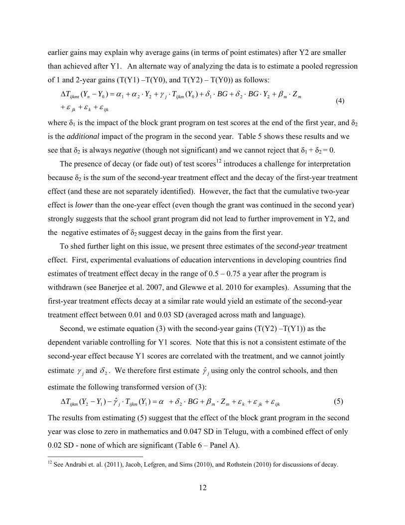
than achieved after Y1. An alternate way of analyzing the data is to estimate a pooled regression
of 1 and 2-year gains (T(Y1) –T(Y0), and T(Y2) – T(Y0)) as follows:
ijkkjk
mmijkmjnijkmt ZYBGBGYTYYYT
22102210 )()(
(4)
where δ1 is the impact of the block grant program on test scores at the end of the first year, and δ2
is the additional impact of the program in the second year. Table 5 shows these results and we
see that δ2 is always negative (though not significant) and we cannot reject that δ1 + δ2 = 0.
The presence of decay (or fade out) of test scores12 introduces a challenge for interpretation
because δ2 is the sum of the second-year treatment effect and the decay of the first-year treatment
effect (and these are not separately identified). However, the fact that the cumulative two-year
effect is lower than the one-year effect (even though the grant was continued in the second year)
strongly suggests that the school grant program did not lead to further improvement in Y2, and
the negative estimates of δ2 suggest decay in the gains from the first year.
To shed further light on this issue, we present three estimates of the second-year treatment
effect. First, experimental evaluations of education interventions in developing countries find
estimates of treatment effect decay in the range of 0.5 – 0.75 a year after the program is
withdrawn (see Banerjee et al. 2007, and Glewwe et al. 2010 for examples). Assuming that the
first-year treatment effects decay at a similar rate would yield an estimate of the second-year
treatment effect between 0.01 and 0.03 SD (averaged across math and language).
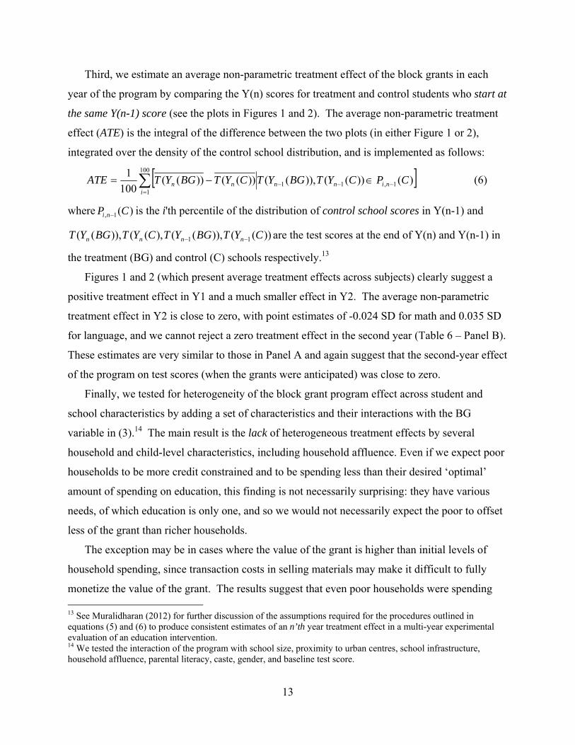
Second, we estimate equation (3) with the second-year gains (T(Y2) –T(Y1)) as the
dependent variable controlling for Y1 scores. Note that this is not a consistent estimate of the
second-year effect because Y1 scores are correlated with the treatment, and we cannot jointly
estimate j and 2 . We therefore first estimate j using only the control schools, and then
estimate the following transformed version of (3):
ijkjkkmmijkmjijkm ZBGYTYYT 2112 )(ˆ)(
(5)
The results from estimating (5) suggest that the effect of the block grant program in the second
year was close to zero in mathematics and 0.047 SD in Telugu, with a combined effect of only
0.02 SD - none of which are significant (Table 6 – Panel A).
12 See Andrabi et. al. (2011), Jacob, Lefgren, and Sims (2010), and Rothstein (2010) for discussions of decay.
13
Third, we estimate an average non-parametric treatment effect of the block grants in each
year of the program by comparing the Y(n) scores for treatment and control students who start at
the same Y(n-1) score (see the plots in Figures 1 and 2). The average non-parametric treatment
effect (ATE) is the integral of the difference between the two plots (in either Figure 1 or 2),
integrated over the density of the control school distribution, and is implemented as follows:
100
11,11 )())(()),(())(())((
100
1
ininnnn CPCYTBGYTCYTBGYTATE (6)
where )(1, CP ni is the i'th percentile of the distribution of control school scores in Y(n-1) and
))(()),((),(()),(( 11 CYTBGYTCYTBGYT nnnn are the test scores at the end of Y(n) and Y(n-1) in
the treatment (BG) and control (C) schools respectively.13
Figures 1 and 2 (which present average treatment effects across subjects) clearly suggest a
positive treatment effect in Y1 and a much smaller effect in Y2. The average non-parametric
treatment effect in Y2 is close to zero, with point estimates of -0.024 SD for math and 0.035 SD
for language, and we cannot reject a zero treatment effect in the second year (Table 6 – Panel B).
These estimates are very similar to those in Panel A and again suggest that the second-year effect
of the program on test scores (when the grants were anticipated) was close to zero.
Finally, we tested for heterogeneity of the block grant program effect across student and
school characteristics by adding a set of characteristics and their interactions with the BG
variable in (3).14 The main result is the lack of heterogeneous treatment effects by several
household and child-level characteristics, including household affluence. Even if we expect poor
households to be more credit constrained and to be spending less than their desired ‘optimal’
amount of spending on education, this finding is not necessarily surprising: they have various
needs, of which education is only one, and so we would not necessarily expect the poor to offset
less of the grant than richer households.
The exception may be in cases where the value of the grant is higher than initial levels of
household spending, since transaction costs in selling materials may make it difficult to fully
monetize the value of the grant. The results suggest that even poor households were spending 13 See Muralidharan (2012) for further discussion of the assumptions required for the procedures outlined in equations (5) and (6) to produce consistent estimates of an n’th year treatment effect in a multi-year experimental evaluation of an education intervention. 14 We tested the interaction of the program with school size, proximity to urban centres, school infrastructure, household affluence, parental literacy, caste, gender, and baseline test score.
14
enough on education so as to substitute away most of the value of the school grant from their
own spending. We verify this by looking at household spending on education in the control
schools and find that only 12% of households report spending less than Rs. 125/year (the value
of the grant) on their child's education, suggesting that the grant was infra-marginal for most
households and could be offset easily.
E. Robustness
The evidence on household spending and test scores is consistent with a model in which
households respond to anticipated school funding. The crowding out of private spending is
sufficiently substantial to lead to no impact on test scores from anticipated school grants, while
unanticipated changes positively impact the growth of test scores of children. We now consider
the robustness of these results to alternative interpretations; in particular, we are interested in
evaluating other potential channels that could have generated similar results, but were unrelated
to behavioral responses among households.
E.1 How different are parental expectations about the grant across the two years?
One possible concern is that the distinction between anticipated and unanticipated funding is
artificial, and households can similarly anticipate both sources after all. This is hard to sustain:
As mentioned earlier, the schools had no reason whatsoever to expect the program in the first
year, while the grant was eagerly anticipated by schools in the second year. Also, as suggested
earlier, most household spending on education occurs at the start of the school year, whereas the
announcement of the grant program was made around one and a half months into the school year
in Y1 and materials were typically procured a few weeks after that. Thus, it is highly likely that
materials bought with the grant supplemented the initial household spending and that the first-
year program effect represents a "production function" effect of additional spending on school
materials. In the second year of the program, field reports suggest that in many cases, parents
were aware of the grant program, and waited to see what materials the school would buy with the
grant before incurring their own expenditures on materials.15 While, we do not explicitly
measure or manipulate expectations, the discussion above suggests a clear difference in the
degree of anticipation of funds in the first and second year.
15 This interpretation is further corroborated by field reports from household interviews after the program was withdrawn, which suggest that around two months into the school year, most parents had not bought the materials that they thought would be provided by the school
15
E.2 What are the components of spending?
A further possible concern regarding our interpretation of the results is that it is possible that
the grants in the first year were spent by schools on items that households cannot substitute for,
while in the second year, the grants were spent on more substitutable items. We show that this is
unlikely to be the case. Spending patterns across various categories are almost identical between
the first and second years of the project and Table 2 clearly shows that the funds were spent on
the same type of inputs both when they were unanticipated (first year) and anticipated (second
year). This also helps rule out explanations based on diminishing returns to the items procured or
the durable nature of school materials. It is possible that some of the classroom materials
purchased may be durable, and the results reflect diminishing returns to durables in the second
year. However, we see that the same fraction of the grant was spent on classroom materials in
both years, suggesting that even these materials needed to be replenished. We also explicitly
record spending on durables (school bags, uniforms, plates, etc.) and find that these accounted
for less than 10% of spending in the first year, and under 1% in the second year.
E.3 Storage and Smoothing
In interpreting our results, a question that arises is whether households or schools could have
smoothed the unexpected grant by either saving some of the funds or storing some materials for
use in later years (if the materials had already been bought). On the school side, the program
design did not provide schools the option of saving funds. They could have saved materials, but
they spend on the same sets of materials in both years suggesting that storage was limited, and
that the grant led to a near one for one increase in learning materials in the first year. On the
household side, we see that they do not reduce their expenditure in response to the unanticipated
grant, but cannot fully rule out the possibility of some storage. But even if some smoothing via
savings, storage, or durable goods spending by the school may have been possible, the
coefficient on the unexpected grant is a lower bound on the production function parameter
(because in this case, the full value of the grant will not have been spent in the same time period)
and our results show that the production function effect of the school grant is positive – which
would not have been apparent if the relationship between school grants and test scores were to
have been estimated using anticipated grants (as we will see again in the Zambia results in
section 4).
16
E.4 Other Budgetary Offsets
A further concern is the possibility that anticipated funds are offset by a reduction of other
transfers to the program schools, which may explain the drop off in the second-year test scores in
the treatment group. We rule this out by measuring the total grants received by the schools from
all other sources and finding that there is no difference in year to year receipts of funds in either
treatment or control schools. There is also no significant difference between the amounts
received in treatment and control schools in any year, or a significant difference between any of
these differences across the years.
E.5 Are parents behaving rationally?
Our results may raise the concern that parents are 'leaving human capital on the table' and
not behaving rationally (as implied by the model). Specifically, if test scores can be increased by
0.09 SD by simply spending an extra $3/year (as indicated by the Y1 results), is it rational for
parents to cut back their own spending in response to the grant and forego these gains to test
scores? The data suggest that parents are not behaving irrationally, and that the extent of the
offset yields an estimate of income elasticity of education spending between 1.8 and 4.6, which
suggests that parents spend a greater share of income on education as income increases (see Das
et al. 2011 for details of the calculation). However, since the grant is fungible when provided in
the form of books and materials, it is rational for households to offset a considerable fraction of
the value of the grant (but not all of it) and to accept a correspondingly lower impact on test
scores than when all the additional income was spent on education (as was the case in Y1). This
impact may be positive, but is not significantly different from zero in our data.16
E.6 Gift Exchange and Hawthorne Effects
A final possibility we consider is that there is no direct link between the increased resources,
the corresponding household responses, and the test-scores findings, but that the test-score
findings are in fact mediated by some other process. One possible narrative could be that the test
score response in Y1 is not a production function effect of the grant, but is instead due to
16 While we did not detect a significant impact on test-scores in Y2, our best estimate of the gain in Y2, the point estimate in column [1] in table 6, suggests a gain of 0.02 SD, or a quarter of the gain in Y1, consistent with a net spending gain in Y2 that was a quarter of that in Y1. As we do not have data on what the households did with the extra resources that were freed up as a result of the school grant, we cannot say much about the welfare impact of the program. However, since the grant was small, it would be difficult to detect significant increases in any particular component of household spending even with more detailed household surveys.
17
increased teacher and school effort in response to receiving a ‘gift’ (as in the gift-exchange
model of Akerlof 1982), whereas in Y2, the schools and teachers get ‘habituated’ to the grant,
and then parents reduce spending while teachers reduce effort (see Gneezy and List 2006 for an
example of this). A related narrative is one of Hawthorne effects whereby the program schools
reacted to the novelty of the program by increasing effort in the first year of the program, but
reverted to usual levels of effort once the novelty wore off.
We are unable to find such patterns in the data. There are no differences in teacher absence or
teaching activity across treatment and control groups in either Y1 or Y2 or within treatment
schools across Y1 and Y2.17 Furthermore, if such a ‘gift exchange’ or ‘novelty’ idea was
empirically relevant, we should expect similar patterns to be present in the other experiments
conducted in the same setting, with considerably higher impact when programs start, but then
dropping off to no impact when schools get habituated to the programs. We find that this is not
the case. In schools provided with an extra contract teacher or with performance-linked pay for
teachers (see Muralidharan and Sundararaman 2011 and 2012 for details), the 2-year effect is
larger than the 1-year effect (and we cannot reject that the 2-year effect is twice the 1-year
effect), and the block grant program is the only one where the 2-year effect is lower than the 1-
year effect. Finally, Muralidharan and Sundararaman (2010) show in the same context that
providing schools with diagnostic feedback and low-stakes monitoring had no impact on test
scores, suggesting that pure Hawthorne effects were unlikely to be an explanation for the
positive test score impact of the block grant program in the first year.
Since teacher inputs (headcount or effort), cannot easily be substituted for by illiterate
parents (while materials can), these results offer further support to our contention that the test
score results in this paper most likely reflect the difference between a situation where households
have not yet re-optimized their spending (Y1) and one where they have (Y2). Overall, the
considerable crowding-out as found in the household spending analysis (Table 3) continues to
offer a consistent, plausible, and parsimonious mechanism to explain our findings that test scores
are significantly higher in program schools at the end of Y1, but not different across treatment
and controls schools at the end of Y2.
A key question in considering the broader relevance of our results is the extent to which they
17 Teacher absence and activity are measured by direct physical observation during unannounced visits to schools with six visits to each treatment and control school in Y1 and four in Y2.
18
can be replicated in other settings. Our data from Zambia allows us to test the main predictions
of the model in a completely different context, and provide two additional advantages beyond
external validity. First, the data come from a nationally scaled-up school grant program
implemented by the Government of Zambia as a 'steady state' policy, and these results may be
more directly relevant to other policy settings. The second advantage is that in addition to the
predictable school grant, we also have data on a much more idiosyncratic source of school
funding, which allows us to test the impact of both unanticipated and anticipated grants on test
scores contemporaneously (whereas it was sequential in AP).
III. Zambia
A. Background and Context
The education system in Zambia is based on public schools (less than 2 percent of all schools
are privately run) and the country has a history of high primary enrollment rates. Teacher salaries
are paid directly by the central government, and account for the majority of spending on school-
level resources; schools receive few other resources from the government. Parental involvement
in schools is high and parents were traditionally expected to contribute considerably to the
finances of the school via fees paid through the Parent Teacher Association (PTA). Limited
direct government funding for non-salary purposes during economic decline put pressure on
parents to provide for inputs more usually provided by government expenditure. This customary
arrangement regarding PTA fees changed in 2001; following an agenda of free education, all
institutionalized parental contributions to schools, including formal PTA fees were banned in
April 2001.
At the same time (in 2001), a rule-based cash grant through the government's Basic
Education Sub-Sector Investment Program (BESSIP) was provided to every school to reverse
some of the pressure on school finances arising from the banning of PTA fees. These grants were
fixed at $600 per school ($650 in the case of schools with Grades 8 and 9) irrespective of school
enrollment to exclude any discretion by the administration. The grant was managed via a
separate funding stream from any other financial flows, and directly delivered to the school, via
the headmaster. Spending decisions were made at the Annual General Meeting, before the start
of the school year. The share of the BESSIP grant in overall school funding was considerable:
for 76% of schools it was the only public funding for non-salary inputs, while its average share
in total school resources was 86%.
19
The scheme also attracted much publicity, which increased its transparency. Combined with
the simplicity of the allocation rule, this ensured that the grants reached their intended recipients.
Disbursement was fast and reliable and 95 percent of all schools had received the stipulated
amounts by the time of the survey and the remainder within 1 month of survey completion (Das
et al. 2003).18 Therefore, we expect that in the year of the survey (2002) the fixed cash grants
would be anticipated by households making their education investment decisions for the year.
Furthermore, because the grants were fixed in size, there was considerable variation across
schools in per-student terms due to underlying differences in enrollment.19
In addition to these predictable rule-based grants, districts also received some discretionary
funding for non-salary purposes from the central government and aid programs. However, since
the 1990s, these sources were highly unreliable and unpredictable, partly due to the operation of
a "cash budget" in view of the poor macroeconomic situation, and partly due to the irregularity of
much of the aid flows to the education sector (Dinh, et al. 2002). In 2002, the year of our survey,
less than 24 percent of all schools received such discretionary grants and conditional on receipt,
there was considerable variation with some schools receiving 30 times as much as others.20
Conversations with district-level officials suggested that it was very difficult for schools to
predict whether these grants would be received (and if so how much), and as we discuss further
below, there does not appear to be any correlation between receipt of these discretionary funds
and observable characteristics of the schools. Overall, the share of discretionary resources was
only about a tenth of the share of the teacher salary bill. Finally, few resources were distributed
in kind to schools during the year of the survey (see Das et. al 2003).
This variation in the per-student rule-based grants as well as the variation in the receipt of
discretionary funds allows us to study the impact of anticipated and unanticipated school grants
on test score gains as discussed below
B. Sampling and Data
We collected data in 2002 from 172 schools in 4 provinces of Zambia (covering 58 percent
of the population), where the schools were sampled to ensure that every enrolled child had an
18This contrasts with the early experience in Uganda (Reinnika and Svensson 2004). 19 The mean transfer per pupil was about $1.2, and the 10th to 90th percentile range of the per-pupil grant was $0.3 to $2.5 confirming the wide variation in the grant amount. 20 The average discretionary transfer per pupil in the sample was about $2.4; conditional on receiving it, this is about $9.8 per pupil.

20
equal probability of inclusion. The school surveys provide basic information on school materials
and funding as well as test scores for mathematics and English for a sample of 20 students in
grade 5 in every school, who were tested in 2001 as part of an independent study and were then
retested in 2002 to form a panel.
A key advance over the existing literature on the impact of school spending on test scores is
our ability to create a matched data set of spending between schools and households. We do this
by collecting education expenditure data from 540 households matched to a sub-sample of 34
schools identified as "remote" using GIS mapping tools (defined as schools where the closest
neighboring school was at least 5 kilometers away). From these schools, the closest village was
chosen and 15 households were randomly chosen from households with at least one child of
school-going age. The restriction of the household survey sample to 34 remote schools allows us
to match household and school inputs in an environment where complications arising from
endogenous school choice are eliminated. We use the entire sample of 172 schools to estimate
the relationship between test scores and cash grants to schools (rule-based and discretionary). We
use the sub-sample of 34 schools matched to 540 households to estimate the relationship between
rule-based cash grants to schools and household expenditures on education.
C. Impact of School Grants on Test Scores
We explore the impact of different types of school grants using Equation (7), based on (1),
modeling changes in standardized test-scores TS between t and t-1 regressed on anticipated and
unanticipated school funds, and a set of controls at t-1 (capturing sources of heterogeneity):
ittujt
ajtoit XwwTS 1321 lnln (7)
In (7), ajw and u
jw are respectively anticipated (from the rule-based BESSIP grant) and
unanticipated (from district-level discretionary sources) grants per student in school j, and Xt-1
are a set of geographic and school level control variables.21 The prediction is that α1 < α2:
unanticipated spending will have a larger effect on test scores than anticipated spending.
We first present results from estimating equation (7) with only the anticipated grant, and our
main result is that there is no correlation between variation in per-student rule-based school
grants and test score gains. We then add an indicator for receipt of discretionary funds (that we
21 Geographic controls include province and rural/urban indicators; school controls include school-level variables such as characteristics of the head-teacher and the head of the Parent-Teacher Association, and PTA fees.
21
argued earlier are difficult to anticipate relative to the rule-based grants) to estimate equation (7)
and test α1 < α2. Recall that there is high variability in discretionary funding, with less than a
quarter of the school sample receiving any funds, and high variance among schools receiving
funds. We therefore present two functional forms - first with an indicator for receipt of any
discretionary funds as a binary variable and second with a continuous measure for the amount of
discretionary funds received, including both linear and quadratic terms.
The first main result we see that there is no correlation between variation in rule-based,
anticipated school grants and test score gains (Table 7 – columns 1 and 4). These results are
similar to those observed in several other contexts and would suggest that “spending does not
matter” for education outcomes. However, when we add an indicator for whether a school
received discretionary funds (that we argued are difficult to anticipate), we find that students in
schools receiving discretionary funds (with a median value of $3/student) gain an additional 0.10
SD in both English and Mathematics test scores (columns 2 and 5). When the discretionary
funds are coded as a continuous variable, we find significant positive effects on English scores,
but do not find any effect on Math scores (columns 3 and 6).22
One key threat to identification in the results above is the possibility that the
discretionary/unanticipated grants may have been targeted to areas with the most potential
improvement in test scores. Alternatively, parents, head teachers, and communities that cared
enough to obtain these funds for their schools may also be motivated to increase test scores in
other ways. We address this concern by comparing the characteristics of schools that do and do
not receive these discretionary funds and find that there is no significant difference between
these types of schools (Table 8 - Column 3). We also test if these observable characteristics can
jointly predict whether a school would have received discretionary funds, and reject the joint
significance of these characteristics (Table 8 - Column 4). While we cannot fully rule out
omitted variable concerns, there is no evidence of differences between schools that do and do not
receive these discretionary funds on observable characteristics.
To summarize, we find that variation in rule-based, well publicized source of funding are
not correlated with test score gains, while less predictable funding sources are. These results
highlight the potentially different impacts of unanticipated and anticipated school funds on test
22 Nonparametric investigation of the relationship between levels of discretionary funds and test score gains suggested a positive, but highly non-linear relationship for both English and Mathematics.
22
score gains, and the importance of making this distinction for empirical work. The second novel
contribution of the empirical work in Zambia to the literature on the impact of school spending
on test scores is our ability to analyze matched data on household and school spending, and study
the possibility of household spending offsets as a possible mechanism for the lack of correlation
between predictable grants and test score gains.
D. Household Spending
We estimate a cross-sectional household expenditure model for the 1195 children (from 540
households) matched to 34 schools in which household spending on school-related inputs is
regressed on anticipated and unanticipated grants with and without a set of controls for child,
household and school-level variables. We estimate:
jii4uj3
aj2i1ij XwlnwlnAzln (8)
where ijz is the spending by the household on child i enrolled in school j, ajw and u
jw are
respectively anticipated (rule-based) and unanticipated (discretionary) grants per student in
school j that matches to child i, and iX are other characteristics of child i including assets owned
by the household. We test 032 , i.e., households respond negatively to the pre-
announced, anticipated rule-based grants at the school level by cutting back their own funding,
but are unable to respond to cash grants that are unanticipated.
We first present OLS results of estimating (8) without and with controls (Table 9 - Columns
1 and 2). However, one concern with OLS could be that ajw captures unobserved components of
household demand operating through an enrollment channel (since the per-child rule-based grant
will be smaller in schools with a larger enrollment). We therefore use the size of the eligible
cohort in the catchment area as an instrument for school enrollment and therefore the level of
per-student cash grants (columns 3 and 4).23 This instrumentation strategy is similar to Case and
Deaton (1999), and Urquiola (2006) in the case of class-size and more recently by Boonperm et
al. (2009) and Kaboski and Townsend (forthcoming) in the context of large fixed grants to
villages in Thailand. Using the size of the eligible cohort as an instrument for enrollment is
especially credible in this context since we use only a sample of remote schools and can abstract
23 The size of the catchment area is defined here as to the total number of children of the relevant age group in the five villages identified by the school as the most important sources of pupils.
23
away from issues of school choice. We also confirm that there is no correlation between the
instrument and iX .24
The results are consistent with the predictions from our model: across all specifications -
OLS and IV - the estimated elasticity of substitution for anticipated grants ( ) is always
negative and significant and ranges from -0.72 to -1.12 while the coefficient of unanticipated
grants ( ) is small and insignificant. Crowding out appears large, and evaluated at the mean we
cannot even reject the hypothesis that for each dollar spent on the rule-based grant per student,
households reduce school expenditure by one dollar, while there is no substitution of
discretionary, unanticipated spending. However, we place less emphasis on the latter result
because only 4 out of the 34 remote schools (where we have household spending data) reported
receiving any of the discretionary funds (whereas all 34 schools received the rule-based grant).
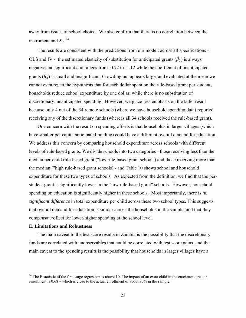
One concern with the result on spending offsets is that households in larger villages (which
have smaller per capita anticipated funding) could have a different overall demand for education.
We address this concern by comparing household expenditure across schools with different
levels of rule-based grants. We divide schools into two categories - those receiving less than the
median per-child rule-based grant ("low rule-based grant schools) and those receiving more than
the median ("high rule-based grant schools) - and Table 10 shows school and household
expenditure for these two types of schools. As expected from the definition, we find that the per-
student grant is significantly lower in the "low rule-based grant" schools. However, household
spending on education is significantly higher in these schools. Most importantly, there is no
significant difference in total expenditure per child across these two school types. This suggests
that overall demand for education is similar across the households in the sample, and that they
compensate/offset for lower/higher spending at the school level.
E. Limitations and Robustness
The main caveat to the test score results in Zambia is the possibility that the discretionary
funds are correlated with unobservables that could be correlated with test score gains, and the
main caveat to the spending results is the possibility that households in larger villages have a
24 The F-statistic of the first stage regression is above 10. The impact of an extra child in the catchment area on enrollment is 0.68 – which is close to the actual enrollment of about 80% in the sample.
24
different demand for education. While we cannot completely rule out these possibilities, Tables
8 and 10 suggest that these concerns may not be first order ones.
Other caveats seem less important. While we cannot attribute school spending to specific
sources of funding (discretionary vs. rule-based), much spending at the school level from both
sources appears to be substitutable. The total shares spent on those items most suitable for
substitution (books, chalks, and stationery) add up to 57% and 47% respectively for schools
without and with discretionary funding, suggesting that in both cases, substantial and similar
spending occurs on items that could be substituted by households.
It is also hard to prove whether the discretionary spending was a true surprise, but the
uncertainty related to the cash-budget meant that actual spending and budgets were far apart. The
typical arrival of these funds at varying points during the school year suggest that households
were unlikely to be able to respond to these (as suggested by the positive test score gains in these
schools in Table 7, and the findings in Table 9). In addition, we see clearly in Table 10 that
households do respond substantially to variations in the rule-based grants and that they spend
much more/less in schools with lower/higher per-student rule-based funding. These different
types of funding were also not used to offset each other. We find no significant correlation
between the amount of rule-based funding and discretionary funding (this can also be seen in
Table 7, where the coefficient on the anticipated rule-based grant is unaffected by the inclusion
of the discretionary grants).
Mirroring the results from the experimental design in AP, but this time from a nationwide
program of school grants, the findings from Zambia suggest that the crowding-out of household
spending in response to a predictable stream of school funds is likely to be an important
mechanism behind the lack of correlation between variation in anticipated school spending and
test scores. While we cannot allay all possible identification concerns with cross-sectional
evidence, the correlations presented are consistent with the model, and the model in turn
provides a parsimonious and consistent framework to interpret the evidence.
IV. Conclusion
Data on test-scores and household expenditures in the context of an experimental school
grant program in the Indian state of Andhra Pradesh suggest that households reduce private
educational spending in response to anticipated school grants, but (by definition and empirically)

25
do not change spending in response to unanticipated grants. They also show that only
unanticipated school grants increase test-scores while anticipated grants have no impact. Cross-
sectional data from a nationally scaled-up school grant program in Zambia are consistent with
the same interpretation. Finding the same result in different countries on different continents,
with different implementing agencies, and in both experimental as well as a scaled-up program
suggests that the issue of household crowd out in the context of public education spending is
likely to be of general relevance for both education research and policy.
This distinction between anticipated and unanticipated inputs could account for the wide
variation in estimated coefficients of school inputs on test scores (Glewwe 2002, Hanushek
2003, Krueger 2003). The typical production function framework does not separate anticipated
from unanticipated inputs and so the regressor is a combination of these two different variables.
Our use of anticipated and unanticipated inputs allows the examination of both effects separately,
thus shedding more light on the process through which school inputs may or may not affect
educational attainments. From a methodological perspective, it is worth noting that while
experimental evaluations of education interventions typically overcome selection and omitted
variable concerns, the distinction highlighted in this paper is relevant even for experiments, since
the interpretation of experimental coefficients depends on the time horizon of the evaluation and
whether this was long enough for other agents to re-optimize their own inputs.
We caution that the evidence presented in this paper is not sufficient to draw a causal link
between the decline in household spending and the lack of an impact of anticipated grants on
test-scores. In particular, we looked for behavioral responses in those components of household
investment that were easiest to measure, which was educational spending. Although we are able
to provide evidence ruling-out a number of other channels, it is possible that parents, children
and teachers also altered the effort that they exerted over the two years of the AP experiment,
and this could have had an independent impact on test-scores.25
Further, our results do not suggest an education policy where inputs are provided
unexpectedly. Although test scores in the current period increase with unanticipated inputs, the
additional consumption will push households off the optimal path. In subsequent periods,
25 Experiments where both information about the program and the type of intervention are experimentally allocated would allow us to better understand the specific role of anticipation (versus, alternate explanations like gift-exchange) and contemporaneously estimate the impact of both anticipated and unanticipated interventions.

26
therefore, they will readjust expenditures until the first-order conditions are valid again –
unanticipated inputs in the current period will not have persistent effects in the future (except due
to the durable nature of some inputs). The policy framework that is suggested under this
approach involves a deeper understanding of the relationship between public and private
spending, acknowledging that this may vary across different components of public spending.
Thus, a policy implication of our results is that schooling inputs that are less likely to be
substituted away by households may be better candidates for government provision. One
important example may be teaching inputs, whereby the combination of economies of scale in
production (relative to private tuition), difficulty of substituting for teacher time by poorly
educated parents, or the generic non-availability of trained personnel in every village could make
public provision more efficient (see Andrabi et al., 2010). In a parallel experiment on the
provision of an extra contract teacher to randomly-selected schools in Andhra Pradesh,
Muralidharan and Sundararaman (2012) find that the impact of the extra teacher was identical in
both the first and second year of the project – suggesting that teacher inputs were less likely to be
substituted away. Another example may be investments in improving classroom pedagogical
processes such as tracking children based on ability (Duflo, Dupas and Kremer 2011 demonstrate
second-year results of a tracking experiment that are larger than those obtained in the first-year).
The approach followed here of treating test scores as a household maximization problem,
with the production function acting as a constraint, explicitly recognizes the centrality of
households in the domain of child learning, with important implications for both estimation and
policy. These issues go beyond the study of the impact of public expenditures on education, but
apply similarly to other areas of public spending, such as health and anti-poverty programs.
More broadly, analysis of the impact of development programs in general will benefit from
paying careful attention to the behavioral responses of households to enrich our understanding of
observed variation in policy impacts in different settings and over different time horizons.

27
References Akerlof, George. 1982. "Labor Contracts as Partial Gift Exchange." Quarterly Journal of
Economics no. 97 (4):543-569. Andrabi, Tahir, Jishnu Das, and Asim Khwaja. 2011. Students Today, Teachers Tomorrow?
Identifying Constraints on the provision of Education. In World Bank Policy Research Working Paper 5674: World Bank.
Andrabi, Tahir, Jishnu Das, Asim Khwaja, and Tristan Zajonc. 2011. "Do Value-Added Estimates Add Value? Accounting for Learning Dynamics." American Economic Journal: Applied Economics no. 3 (July):29-54.
Autor, David H., and Mark G. Duggan. 2003. "The Rise in The Disability Rolls And The Decline In Unemployment." The Quarterly Journal of Economics no. 118 (1):157-205.
Banerjee, Abhijit, Shawn Cole, Esther Duflo, and Leigh Linden. 2007. "Remedying Education: Evidence from Two Randomized Experiments in India." Quarterly Journal of Economics no. 122 (3):1235-1264.
Becker, Gary S, and Nigel Tomes. 1976. "Child Endowments and the Quantity and Quality of Children." Journal of Political Economy no. 84 (4):S143-S162.
Boonperm, Jirawan, Jonathan Haughton, and Shahidur R. Khandker. 2009. Does the Village Fund Matter in Thailand? : The World Bank.
Case, Anne, and Angus Deaton. 1999. "School Inputs and Educational Outcomes in South Africa." Quarterly Journal of Economics no. 114 (3):F1047-F84.
Cutler, David M., and Jonathan Gruber. 1996. "The Effect of Medicaid Expansions on Public Insurance, Private Insurance, and Redistribution." The American Economic Review no. 86 (2):378-383.
Das, Jishnu, Stefan Dercon, James Habyarimana, and Pramila Krishnan. 2003. Rules vs. Discretion: Public and Private Funding in Zambian Education. Development Research Group, The World Bank.
Das, Jishnu, Stefan Dercon, James Habyarimana, Pramila Krishnan, Karthik Muralidharan, and Venkatesh Sundararaman. 2011. School Inputs, Household Substitution, and Test Scores. National Bureau of Economic Research Working Paper 16830.
Deaton, Angus, and John Muellbauer. 1980. Economics and Consumer Behavior. Cambridge, UK: Cambridge University Press.
Dercon, Stefan;, and Pamela Krishnan. 2000. "In Sickness and in Health: Risk Sharing within Rural Households in Rural Ethiopia." Journal of Political Economy no. 108 (4):688-727.
Dinh, Hinh T., Abebe Adugna, and Bernard Myers. 2002. The Impact of Cash Budgets on Poverty Reduction in Zambia: A Case Study of the Conflict between Well-Intentioned Macroeconomic Policy and Service Delivery to the Poor. The World Bank.
Duflo, Esther, Pascaline Dupas, and Michael Kremer. 2011. "Peer Effects, Teacher Incentives, and the Impact of Tracking: Evidence from a Randomized Evaluation in Kenya." American Economic Review no. 101 (5):1739-74.
———. 2012. School Governance, Teacher Incentives, and Pupil-Teacher Ratios: Experimental Evidence from Kenyan Primary Schools. National Bureau of Economic Research. Working Paper 17939.
Eissa, Nada, and Jeffrey B. Liebman. 1996. "Labor Supply Response to the Earned Income Tax Credit." The Quarterly Journal of Economics no. 111 (2):605-637.
Foster, Andrew D. 1995. "Prices, Credit Markets and Child Growth in Low-Income Rural Areas." The Economic Journal no. 105 (430):551-570.
28
Glewwe, Paul. 2002. "Schools and Skills in Developing Countries: Education Policies and Socioeconomic Outcomes " Journal of Economic Literature no. 40 (2):436-482.
Glewwe, Paul, Nauman Ilias, and Michael Kremer. 2010. "Teacher Incentives." American Economic Journal: Applied Economics no. 2 (3):205-227.
Glewwe, Paul, and Michael Kremer. 2006. "Schools, Teachers, and Education Outcomes in Developing Countries." In Handbook of the Economics of Education, edited by Eric Hanushek and Finis Welch. North-Holland.
Glewwe, Paul, Michael Kremer, and Sylvie Moulin. 2009. "Many Children Left Behind? Textbooks and Test Scores in Kenya." American Economic Journal: Applied Economics no. 1 (1):112-135.
Gneezy, Uri, and John List. 2006. "Putting Behavioral Economics to Work: Field Evidence on Gift Exchange." Econometrica no. 74 (5):1365-1384.
Hanushek, Eric A. 2002. "Publicly Provided Education." In Handbook of Public Economics, edited by Alan J Auerbach and Martin S Feldstein, 2045-2141. Amsterdam: North-Holland.
———. 2003. "The Failure of Input-Based Schooling Policies." Economic Journal no. 113 (485):F64-98.
Hanushek, Eric, and Javier A. Luque. 2003. "Efficiency and Equity in Schools around the World." Economics of Education Review no. 20 (5):481-502.
Houtenville, Andrew J., and Karen Smith Conway. 2008. "Parental Effort, School Resources, and Student Achievement." Journal of Human Resources no. 43 (2):437-453.
Jacob, Brian, Lars Lefgren, and David Sims. 2010. "The Persistence of Teacher-Induced Learning Gains." Journal of Human Resources no. 45 (4):915-943.
Jacoby, Hanan G. 2002. "Is There an Intrahousehold 'Flypaper Effect'? Evidence from a School Feeding Programme." The Economic Journal no. 112 (476):196-221.
Jacoby, Hanan G.;, and Emmanuel Skoufias. 1997. "Risk, Financial Markets, and Human Capital in a Developing Country." The Review of Economic Studies no. 64 (3):311-335.
Kaboski, Joseph P., and Robert M. Townsend. Forthcoming. "A Structural Evaluation of a Large-Scale Quasi-Experimental Microfinance Initiative." Econometrica.
Kremer, Michael, Karthik Muralidharan, Nazmul Chaudhury, F. Halsey Rogers, and Jeffrey Hammer. 2005. "Teacher Absence in India: A Snapshot." Review of 2005. Journal of the European Economic Association no. 3 (2-3):658-67.
Krueger, Alan. 2003. "Economic Considerations and Class Size." Economic Journal no. 113:34-63.
Liu, Haiyong, Thomas A Mroz, and Wilbert van der Klaauw. 2010. "Maternal employment, migration, and child development." Journal of Econometrics (156):212-228.
Meyer, Bruce D. 1990. "Unemployment Insurance and Unemployment Spells." Econometrica no. 58 (4):757-782.
Moffitt, Robert A. 2002. "Welfare Programs and Labor Supply." In Handbook of Public Economics, 2393-2430. Elsevier B.V.
Muralidharan, Karthik. 2012. Long Term Effects of Teacher Performance Pay: Experimental Evidence from India. UC San Diego.
Muralidharan, Karthik, and Venkatesh Sundararaman. 2010. "The Impact of Diagnostic Feedback to Teachers on Student Learning: Experimental Evidence from India." Economic Journal no. 120 (546):F187-F203.

29
———. 2011. "Teacher Performance Pay: Experimental Evidence from India." Journal of Political Economy no. 119 (1):39-77.
———. 2012. Contract Teachers: Experimental Evidence from India. UC San Diego. Pop-Eleches, Christian, and Miguel Urquiola. 2011. Going to a Better School: Effects and
Behavioral Responses. National Bureau of Economic Research. Working Paper 16886. Powell, Christine A., Susan P Walker, Susan M Chang, and Grantham-McGregor Sally M.
1998. "Nutrition and education: a randomized trial of the effects of breakfast in rural primary school children." American Journal of Clinical Nutrition no. 68:873–9.
Pratham. 2010. Annual Status of Education Report. Pritchett, Lant, and Deon Filmer. 1999. "What Education Production Functions Really Show: A
Positive Theory of Education Expenditures." Economics of Education Review no. 18 (2):223-39.
Reinikka, Ritva, and Jakob Svensson. 2004. "Local Capture: Evidence From a Central Government Transfer Program in Uganda." The Quarterly Journal of Economics no. 119 (2):679-705.
Rothstein, Jesse. 2010. "Teacher Quality in Educational Production: Tracking, Decay, and Student Achievement." Quarterly Journal of Economics no. 125 (1):175-214.
Todd, Petra E, and Kenneth I Wolpin. 2003. "On the Specification and Estimation of the Production Function for Cognitive Achievement." Economic Journal no. 113 (485):F3-33.
Urquiola, Miguel. 2006. "Identifying Class Size Effects in Developing Countries: Evidence from Rural Bolivia." Review of Economics and Statistics no. 88 (1):171-177.
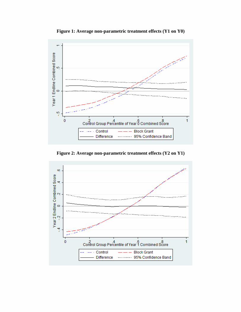
Figure 1: Average non-parametric treatment effects (Y1 on Y0)
Figure 2: Average non-parametric treatment effects (Y2 on Y1)
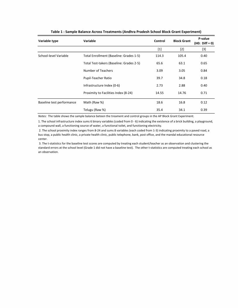
Variable type Variable Control Block GrantP‐value
(H0: Diff = 0)
[1] [2] [3]
School‐level Variable Total Enrollment (Baseline: Grades 1‐5) 114.3 105.4 0.40
Total Test‐takers (Baseline: Grades 2‐5) 65.6 63.1 0.65
Number of Teachers 3.09 3.05 0.84
Pupil‐Teacher Ratio 39.7 34.8 0.18
Infrastructure Index (0‐6) 2.73 2.88 0.40
Proximity to Facilities Index (8‐24) 14.55 14.76 0.71
Baseline test performance Math (Raw %) 18.6 16.8 0.12
Telugu (Raw %) 35.4 34.1 0.39
3. The t‐statistics for the baseline test scores are computed by treating each student/teacher as an observation and clustering the
standard errors at the school level (Grade 1 did not have a baseline test). The other t‐statistics are computed treating each school as
an observation.
Notes: The table shows the sample balance beteen the treament and control groups in the AP Block Grant Experiment.
1. The school infrastructure index sums 6 binary variables (coded from 0 ‐ 6) indicating the existence of a brick building, a playground,
a compound wall, a functioning source of water, a functional toilet, and functioning electricity.
2. The school proximity index ranges from 8‐24 and sums 8 variables (each coded from 1‐3) indicating proximity to a paved road, a
bus stop, a public health clinic, a private health clinic, public telephone, bank, post office, and the mandal educational resource
center.
Table 1 : Sample Balance Across Treatments (Andhra Pradesh School Block Grant Experiment)
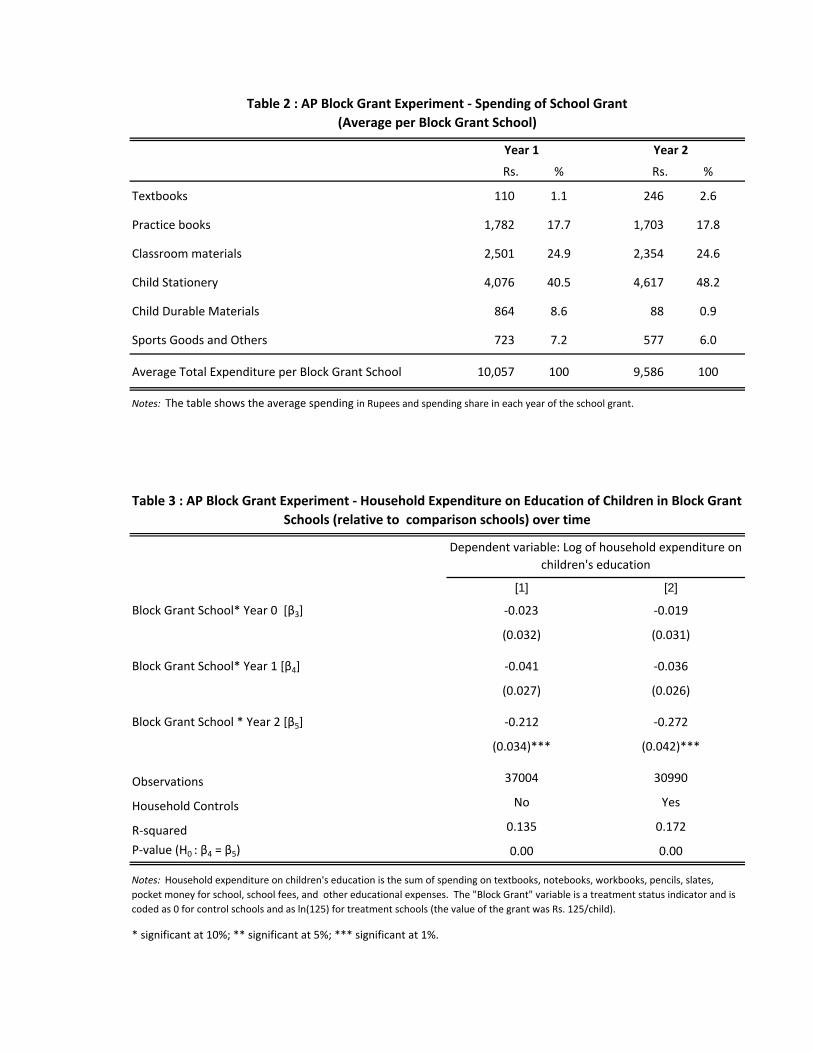
Rs. % Rs. %
Textbooks 110 1.1 246 2.6
Practice books 1,782 17.7 1,703 17.8
Classroom materials 2,501 24.9 2,354 24.6
Child Stationery 4,076 40.5 4,617 48.2
Child Durable Materials 864 8.6 88 0.9
Sports Goods and Others 723 7.2 577 6.0
Average Total Expenditure per Block Grant School 10,057 100 9,586 100
Block Grant School* Year 0 [β3]
Block Grant School* Year 1 [β4]
Block Grant School * Year 2 [β5]
Observations
Household Controls
R‐squared
P‐value (H0 : β4 = β5)
[1] [2]
Table 2 : AP Block Grant Experiment ‐ Spending of School Grant
(Average per Block Grant School)
Year 1 Year 2
Dependent variable: Log of household expenditure on
children's education
Table 3 : AP Block Grant Experiment ‐ Household Expenditure on Education of Children in Block Grant
Schools (relative to comparison schools) over time
Notes: The table shows the average spending in Rupees and spending share in each year of the school grant.
* significant at 10%; ** significant at 5%; *** significant at 1%.
Notes: Household expenditure on children's education is the sum of spending on textbooks, notebooks, workbooks, pencils, slates,
pocket money for school, school fees, and other educational expenses. The "Block Grant" variable is a treatment status indicator and is
coded as 0 for control schools and as ln(125) for treatment schools (the value of the grant was Rs. 125/child).
‐0.023
(0.032)
‐0.041
(0.027)
‐0.212
(0.034)***
37004
0.135
0.00
‐0.019
(0.031)
‐0.036
(0.026)
‐0.272
(0.042)***
30990
0.172
0.00
No Yes
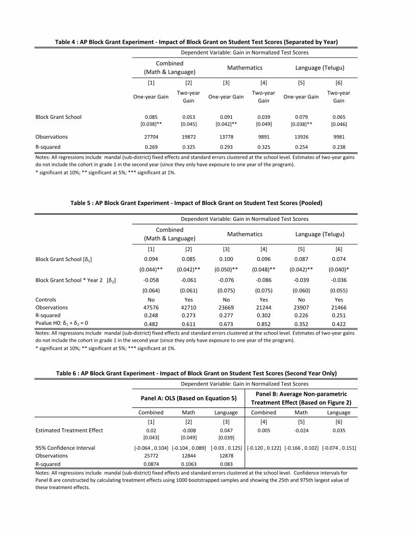
[1] [2] [3] [4] [5] [6]
One‐year GainTwo‐year
GainOne‐year Gain
Two‐year
GainOne‐year Gain
Two‐year
Gain
Block Grant School 0.085 0.053 0.091 0.039 0.079 0.065
[0.038]** [0.045] [0.042]** [0.049] [0.038]** [0.046]
Observations 27704 19872 13778 9891 13926 9981
R‐squared 0.269 0.325 0.293 0.325 0.254 0.238
[1] [2] [3] [4] [5] [6]
Block Grant School [δ1] 0.094 0.085 0.100 0.096 0.087 0.074
(0.044)** (0.042)** (0.050)** (0.048)** (0.042)** (0.040)*
Block Grant School * Year 2 [δ2] ‐0.058 ‐0.061 ‐0.076 ‐0.086 ‐0.039 ‐0.036
(0.064) (0.061) (0.075) (0.075) (0.060) (0.055)
Controls No Yes No Yes No Yes
Observations 47576 42710 23669 21244 23907 21466
R‐squared 0.248 0.273 0.277 0.302 0.226 0.251
Pvalue H0: δ1 + δ2 = 0 0.482 0.611 0.673 0.852 0.352 0.422
Combined Math Language Combined Math Language
[1] [2] [3] [4] [5] [6]
Estimated Treatment Effect 0.02 ‐0.008 0.047 0.005 ‐0.024 0.035
[0.043] [0.049] [0.039]
95% Confidence Interval [‐0.064 , 0.104] [‐0.104 , 0.089] [‐0.03 , 0.125] [‐0.120 , 0.122] [‐0.166 , 0.102] [‐0.074 , 0.151]
Observations 25772 12844 12878
R‐squared 0.0874 0.1063 0.083
Notes: All regressions include mandal (sub‐district) fixed effects and standard errors clustered at the school level. Confidence intervals for
Panel B are constructed by calculating treatment effects using 1000 bootstrapped samples and showing the 25th and 975th largest value of
these treatment effects.
* significant at 10%; ** significant at 5%; *** significant at 1%.
Table 6 : AP Block Grant Experiment ‐ Impact of Block Grant on Student Test Scores (Second Year Only)
Dependent Variable: Gain in Normalized Test Scores
Panel A: OLS (Based on Equation 5)Panel B: Average Non‐parametric
Treatment Effect (Based on Figure 2)
Table 4 : AP Block Grant Experiment ‐ Impact of Block Grant on Student Test Scores (Separated by Year)
Dependent Variable: Gain in Normalized Test Scores
Notes: All regressions include mandal (sub‐district) fixed effects and standard errors clustered at the school level. Estimates of two‐year gains
do not include the cohort in grade 1 in the second year (since they only have exposure to one year of the program).
Combined
(Math & Language)Language (Telugu)Mathematics
Table 5 : AP Block Grant Experiment ‐ Impact of Block Grant on Student Test Scores (Pooled)
Dependent Variable: Gain in Normalized Test Scores
Combined
(Math & Language)Mathematics Language (Telugu)
Notes: All regressions include mandal (sub‐district) fixed effects and standard errors clustered at the school level. Estimates of two‐year gains
do not include the cohort in grade 1 in the second year (since they only have exposure to one year of the program).
* significant at 10%; ** significant at 5%; *** significant at 1%.

[1] [2] [3] [4] [5] [6]
‐0.024 ‐0.018 ‐0.016 ‐0.010 ‐0.004 ‐0.006
[0.031] [0.030] [0.031] [0.025] [0.026] [0.026]
0.103** 0.098*
[0.050] [0.048]
0.060** 0.029
[0.027] [0.024]
‐0.004* ‐0.001
[0.002] [0.002]
Observations 171 171 171 171 171 171
R‐squared 0.17 0.187 0.192 0.044 0.06 0.065
Dependent variable: Gain in normalized test‐scores
Table 7 : Zambia ‐ The Relative Impacts of Rule‐Based Funds and the Receipt of Discretionary Funds on
Test‐Score Gains
Notes : The table reports the estimated effects of rule‐based and discretionary funds on yearly changes in English and
Mathematics test‐scores. Columns 1 and 4 include only the rule‐based grants, while columns 2 and 5 also include an indicator
for receipt of Discretionary Funds. Columns 2 and 5 treat Discretionary Funds as a binary variable, separating schools into
those who received a positive amount versus those who received nothing (rule‐based funds are treated as a continuous
variable). Columns 3 and 6 treat both Discretionary Funds and Rule‐Based Funds as a continuous variable and includes linear
and quadratic terms for the discretionary funds. All specifications include a set of geographical (province and rural/urban
indicators) and school controls (including changes in school‐level variables such as the head‐teacher, the head of the Parent‐
Teacher Association and PTA fees). All standard errors are clustered at the district‐level. *** p<0.01, ** p<0.05, * p<0.1
Any Discretionary Funds Received
(Binary)
Rule‐Based Funds
English Mathematics
Discretionary Funds (in Kwacha per
pupil)
Square of Discretionary Funds (in
Kwacha per pupil)
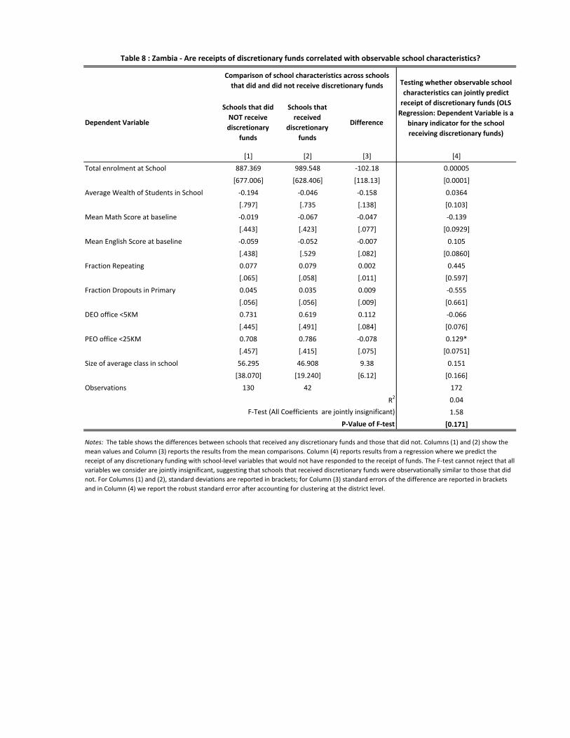
Dependent Variable
Schools that did
NOT receive
discretionary
funds
Schools that
received
discretionary
funds
Difference
[1] [2] [3] [4]
Total enrolment at School 887.369 989.548 ‐102.18 0.00005
[677.006] [628.406] [118.13] [0.0001]
Average Wealth of Students in School ‐0.194 ‐0.046 ‐0.158 0.0364
[.797] [.735 [.138] [0.103]
Mean Math Score at baseline ‐0.019 ‐0.067 ‐0.047 ‐0.139
[.443] [.423] [.077] [0.0929]
Mean English Score at baseline ‐0.059 ‐0.052 ‐0.007 0.105
[.438] [.529 [.082] [0.0860]
Fraction Repeating 0.077 0.079 0.002 0.445
[.065] [.058] [.011] [0.597]
Fraction Dropouts in Primary 0.045 0.035 0.009 ‐0.555
[.056] [.056] [.009] [0.661]
DEO office <5KM 0.731 0.619 0.112 ‐0.066
[.445] [.491] [.084] [0.076]
PEO office <25KM 0.708 0.786 ‐0.078 0.129*
[.457] [.415] [.075] [0.0751]
Size of average class in school 56.295 46.908 9.38 0.151
[38.070] [19.240] [6.12] [0.166]
Observations 130 42 172
0.04
1.58
[0.171]
Table 8 : Zambia ‐ Are receipts of discretionary funds correlated with observable school characteristics?
Notes: The table shows the differences between schools that received any discretionary funds and those that did not. Columns (1) and (2) show the
mean values and Column (3) reports the results from the mean comparisons. Column (4) reports results from a regression where we predict the
receipt of any discretionary funding with school‐level variables that would not have responded to the receipt of funds. The F‐test cannot reject that all
variables we consider are jointly insignificant, suggesting that schools that received discretionary funds were observationally similar to those that did
not. For Columns (1) and (2), standard deviations are reported in brackets; for Column (3) standard errors of the difference are reported in brackets
and in Column (4) we report the robust standard error after accounting for clustering at the district level.
F‐Test (All Coefficients are jointly insignificant)
R2
P‐Value of F‐test
Comparison of school characteristics across schools
that did and did not receive discretionary funds Testing whether observable school
characteristics can jointly predict
receipt of discretionary funds (OLS
Regression: Dependent Variable is a
binary indicator for the school
receiving discretionary funds)
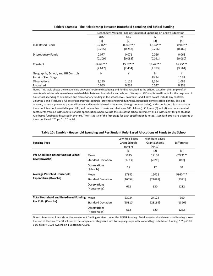
OLS OLS IV IV
[1] [2] [3] [4]
Rule Based Funds ‐0.716** ‐0.843*** ‐1.124*** ‐0.946**
[0.285] [0.252] [0.266] [0.460]
Discretionary Funds 0.077 0.071 0.066 0.063
[0.109] [0.083] [0.091] [0.080]
Constant 14.69*** 15.52*** 18.42*** 16.25***
[2.617] [2.454] [2.383] [3.561]
Geographic, School, and HH Controls N Y N Y
F‐stat of First Stage 23.54 10.32
Observations 1,195 1,116 1,164 1,085
R‐squared 0.053 0.239 0.037 0.238
Funding Type
Low Rule‐based
Grant Schools
(N=17)
High Rule‐based
Grant Schools
(N=17)
Difference
[1] [2] [3]
Mean 5915 12158 ‐6243***
Standard Deviation [1733] [2893] [818]
Observations
(Schools)17 17 34
Mean 17882 12022 5860***
Standard Deviation [26054] [22695] [1391]
Observations
(Households)612 620 1232
Mean 23734 24124 ‐390
Standard Deviation [25810] [23164] [1396]
Observations
(Households)612 620 1232
Per‐Child Rule‐Based funds at School
Level (Kwacha)
Total Household and Rule‐Based Funding
Per Child (Kwacha)
Notes: Rule‐based funds show the per‐student funding received under the BESSIP funding. Total household and rule‐based funding shows
the sum of the two. The 34 schools in the sample are categorized into two equal groups with low and high rule‐based funding. *** p<0.01.
1 US dollar = 3570 Kwacha on 1 September 2001.
Table 9 : Zambia ‐ The Relationship between Household Spending and School Funding
Notes: This table shows the relationship between household spending and funding received at the school, based on the sample of 34
remote schools for whom we have matched data between households and schools. We report OLS and IV coefficients for the response of
household spending to rule‐based and discretionary funding at the school‐level. Columns 1 and 3 have do not include any controls.
Columns 2 and 4 include a full set of geographical controls (province and rural dummies), household controls (child gender, age, age‐
squared, parental presence, parental literacy and household wealth measured through an asset index), and school controls (class‐size in
the school, textbooks available per child, and the number of desks and chairs per 100 children). Columns (3) and (4) are the estimated
coefficients from an instrumental variable specification where we use the size of the school catchment as an instrument for per‐student
rule‐based funding as discussed in the text. The F‐statistic of the first‐stage for each specification is noted. Standard errors are clustered at
the school level. *** p<.01, ** p<.05.
Dependent Variable: Log of Household Spending on Child's Education
Table 10 : Zambia ‐ Household Spending and Per‐Student Rule‐Based Allocations of Funds to the School
Average Per‐Child Household
Expenditure (Kwacha)