Scheduling and Capacity Estimation in · PDF fileScheduling and Capacity Estimation in LTE ... we estimate the total cell throughput/capacity by taking the ... modulation for uplink

ADVANCES IN ELECTRONICS AND TELECOMMUNICATIONS, VOL. 2, NO. 3, SEPTEMBER 2011 31

Scheduling and Capacity Estimation in LTEOlav Østerbø

Abstract—Due to the variation of radio condition in LTEthe obtainable bitrate for active users will vary. The twomost important factors for the radio conditions are fading andpathloss. By considering analytical analysis of the LTE conditionsincluding both fast fading and shadowing and attenuation dueto distance we have developed a model to investigate obtainablebitrates for customers randomly located in a cell. In additionwe estimate the total cell throughput/capacity by taking thescheduling into account. The cell throughput is investigated forthree types of scheduling algorithms; Max SINR, Round Robinand Proportional Fair where also fairness among users is partof the analysis. In addition models for cell throughput/capacityfor a mix of Guaranteed Bit Rate (GBR) and Non-GBR greedyusers are derived.

Numerical examples show that multi-user gain is large for theMax-SINR algorithm, but also the Proportional Fair algorithmgives relative large gain relative to plain Round Robin. The Max-SINR has the weakness that it is highly unfair when it comes tocapacity distribution among users. Further, the model visualizethat use of GBR for high rates will cause problems in LTE dueto the high demand for radio resources for users with low SINR,at cell edge. Persistent GBR allocation will be a waste of capacityunless for very thin streams like VoIP. For non-persistent GBRallocation the allowed guaranteed rate should be limited.

Index Terms—LTE, scheduling, capacity estimation, GBR.

I. INTRODUCTION

THE LTE (Long Term Evolution) standardized by 3GPP isbecoming the most important radio access technique for

providing mobile broadband to the mass marked. The intro-duction of LTE will bring significant enhancements comparedto HSPA (High Speed Packet Access) in terms of spectrumefficiency, peak data rate and latency. Important features ofLTE are MIMO (Multiple Input Multiple Output), higher ordermodulation for uplink and downlink, improvements of layer 2protocols, and continuous packet connectivity [1].

While HSPA mainly is optimized data transport, leaving thevoice services for the legacy CS (Circuit Switched) domain,LTE is intended to carry both real time services like VoIP inaddition to traditional data services. The mix of both real timeand non real time traffic in a single access network requiresspecific attention where the main goal is to maximize cellthroughput while maintaining QoS and fairness both for usersand services. Therefore radio resource management will be akey part of modern wireless networks. With the introductionof these mobile technologies, the demand for efficient resourcemanagement schemes has increased.

The first issue in this paper is to consider the bandwidthefficiency for a single user in cell for the basic unit of radioresources, i.e. for a RB (Resource Block) in LTE. Since LTEuses advanced coding like QPSK, 16QAM, and 64QAM, the

O. Østerbø is with Telenor, Corporate Development, Fornebu, Oslo, Nor-way, (phone: +4748212596; e-mail: [email protected])

obtainable data rate for users will vary accordingly dependingon the current radio conditions. The average, higher momentsand distribution of the obtainable data rate for a user eitherlocated at a given distance or randomly located in a cell, willgive valuable information of the expected cell performance.To find the obtainable bitrate we chose a truncated anddownscaled version on Shannon formula which is in line withwhat is expected from real implementations and also complywith the fact that the maximal bitrate per frequency or symbolfor 64 QAM is at most 6 [2].

For the bandwidth efficiency, where we only consider asingle user, the scheduling is without any significance. Thisis not the case when several users are competing for theavailable radio resources. The scheduling algorithms studied inthis paper are those only depending on the radio conditions, i.e.opportunistic scheduling where the scheduled user determinedby a given metrics which depends on the SINR (signal-to-interference-plus-noise ratio). The most commonly knownopportunistic scheduling algorithms are of this type like PF(Proportional Fair), RR (Round Robin) and Max-SINR. Themethodology developed will, however, will apply for generalscheduling algorithms where the scheduling metrics for a useris given by a known function of SINR, however, now the SINRmay vary in different scheduling intervals taking rapid fadinginto account. The cell capacity distribution is found for caseswhere the locations of the users all are known or as an averagewhere all the users are randomly located in the cell [3].

Also the multi user gain (relative increase in cell throughput)due to the scheduling is of main interest. The proposed modelsdemonstrate the magnitude of this gain. As for Max SINRalgorithm this gain is expected to be huge, however, the gaincomes always at a cost of fairness among users. And thereforefairness has to be taken into account when evaluating theperformance of scheduling algorithms.

It is likely that LTE will carry both real time traffic andelastic traffic. We also analyze scenarios where a cell is loadedby two traffic types; high priority CBR (Constant Bit Rate)traffic that requires a fixed data-rate and low priority (greedy)data sources that always consume the leftover capacity notused by the CBR traffic. This is actual a very realistic trafficscenario for future LTE networks where we will have a mix ofboth real time traffic like VoIP and data traffic. We analyse thiscase by first estimate the RB usage of the high priority CBRtraffic, and then subtract the corresponding RBs to find theactual numbers of RBs available for the (greedy) data trafficsources. Finally we then estimate the cell capacity as the sumof the bitrates offered to the CBR and (greedy) data sources.

The remainder of this paper is organized as follows. Insection II the basic radio model is given and models forbandwidth efficiency are discussed. Section III gives an outlineof the multiuser case where resource allocation and scheduling

32 ADVANCES IN ELECTRONICS AND TELECOMMUNICATIONS, VOL. 2, NO. 3, SEPTEMBER 2011

is taking into account. Some numerical examples are given insection IV and in section V some conclusions are given.

II. SPECTRUM EFFICIENCY

A. Obtainable bitrate per symbol rate as function of SINR

For LTE the obtainable bitrate per symbol rate will dependon the radio signal quality (both for up-and downlink). Theactual radio signal quality is signaled over the radio interfaceby the so-called CQI (Channel Quality Indicator) index inthe range 1 to 15. Based on the CQI value the coding rateis determined on basis of the modulation QPSK, 16QAM,64QAM and the amount of redundancy included. The cor-responding bitrate per bandwidth is standardized by 3GPP [4]and is shown in Table 1 below. For analytical modeling theactual CQI measurement procedures are difficult to incorporateinto the analysis due to the time lag, i.e. the signaled CQI isbased measurements taken in earlier TTIs (Transmission TimeInterval). To simplify the analyses, we assume that this timelag is set to zero and that the CQI is given as a function of themomentary SINR, i.e. CQI=CQI(SINR). This approximationis justified if the time variation in SINR is significantly slowerthan the length of a TTI interval. Hence, by applying the CQItable found in [4] we get the obtainable bitrate per bandwidthas function of the SINR as the step function:

B = fcj , for SINR ∈ [gj , gj+1) ; j = 0, 1, ..., 15, (1)

where f is the bandwidth of the channel, cj is the efficiencyfor QCI equal j (as given by Table 1) and [gj , gj+1) are thecorresponding intervals of SINR values. (We also take c0 = 0,g0 = 0 and g16 =∞.)

To fully describe the bitrate function above we also have toalso specify the intervals [gj , gj+1). Several simulation studiese.g. [5] suggest that there is a linear relation between the CQIindex and the actual SINR limits in [dB]. With this assumptionwe have SINRj [dB] = 10 log10 gj = aj + b or gj = 10

aj+b10

for some constants a and b. It is also argued that the actualrange of the SINR limits in [dB] is determined by thefollowing (end point) observations: SINR[dB]=-6 correspondsto QCI=1, while SINR[dB]=20 corresponds to CQI=15. Hencewe then have −6 = a+ b and 20 = 15a+ b or a = 13/7 andb = −55/7.

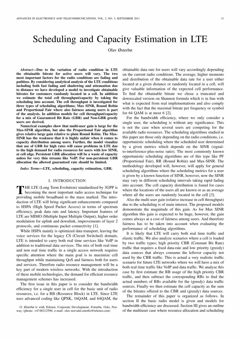
For extensive analytical modelling the step based bandwidthfunction is cumbersome to apply. An absolute upper boundyields the Shannon formula B = f log2(1+SINR), however,we know that the Shannon upper limit is too optimistic.First of all the bandwidth function should never exceed thehighest rate c15 = 5.5547. We therefore suggest downscalingand truncating the Shannon formula and take an alternativebandwidth function as:

B = dmin[T, ln(1 + γSINR)], (2)

with d = f Cln 2 and T = c15 ln 2

C where C is the downscalingconstant (relative to the Shannon formula) and γ is a constantless than unity. By choosing C and γ that minimize the squaredistances between the CQI based and the truncated Shannonformula (2) above we find C = 0.9449 and γ = 0.4852.(Upper and lower estimates of the CQI based zigzagging

TABLE ITABLE 1 CQI TABLE.

CQI index modulation code rate x 1024 efficiency0 out of range

1 QPSK 78 0.15232 QPSK 120 0.23443 QPSK 193 0.37704 QPSK 308 0.60165 QPSK 449 0.87706 QPSK 602 1.17587 16QAM 378 1.47668 16QAM 490 1.91419 16QAM 616 2.406310 64QAM 466 2.730511 64QAM 567 3.322312 64QAM 666 3.902313 64QAM 772 4.523414 64QAM 873 5.115215 64QAM 948 5.5547

0 5 10 15 20 25SINR @dBD

1

2

3

4

5

6

de

si

la

mr

oN

tu

ph

gu

or

hT

@t

ib

êsêz

HD

---- Shannon

---- Modified Shannon

---- LTE CQI table

Fig. 1. Normalized throughput as function of the SINR based on: 1.-QCItable, 2.-Shannon and 3.-Modified Shannon.

bitrate function is obtained by taking γu = γ10a/20 = 0.6008and γl = γ10−a/20 = 0.3918).

We observe that a downscaling of the Shannon limit is verymuch in line with the corresponding bitrates obtained by theCQI table as shown in Figure 1 and hence we believe that (2)yields a quite accurate approximation. In fact the approximatedCQI values cappj follow the similar logarithmic behaviour:

cappj = C log2(1 + αβj), (3)

where now have α = γ10a/20+b/10 = 0.0984 and β =10a/10 = 1.5336.

B. Radio channel models

Generally, the SINR for a user will be the ratio of thereceived signal strength divided by the corresponding noise.The received signal strength is the product of the power Pwtimes path loss G and divided by the noise component N ,i.e. SINR = PwG

N . Now the path loss G will typical be astochastic variable depending on physical characteristics such

ØSTERBØ: SCHEDULING AND CAPACITY ESTIMATION IN LTE 33

as rapid and slow fading, but will also have a componentthat are dependent on distance (and possible also the sendingfrequency). Hence, we first consider variations that are slowlyvarying over time intervals that are relative long comparedwith the TTIs (Transmission Time Intervals). Then the pathloss is usually given in dB on the form:

G = 10L/10 with L = C −A log10(r) +Xt, (4)

where C and A are constants, A typical in the range 20-40, andXt a normal stochastic process with zero mean representingthe shadowing (slow fading). The other important componentdetermining the SINR is the noise. It is common to splitthe noise power into two terms: N = Nint + Next whereNint is the internal (or own-cell) noise power and Next isthe external (or other-cell) interference. In a CDMA (CodeDivision Multiple Access) network, the lack of orthogonalityinduces own-cell interference. In an OFDMA (OrthogonalFrequency Division Multiple Access) network, however, thereis a perfect orthogonality between users and therefore theonly contribution to Nint is the terminal noise at the receiver.The interference from other cells depends on the location ofsurrounding base stations and will typically be largest at celledges. In the following we shall assume that the external noiseis constant throughout the cell or negligible, i.e. we assumethe noise N to be constant throughout the cell.

Hence, with the assumptions above, we may write SINR onthe form St/h(r, λ) where St represent the stochastic varia-tions which we assume to be distance independent capturingthe slowly varying fading, and h(r, λ) represent the distancedependant attenuation (which we also allow to depend on thesending frequency). Most commonly used channel models asdescribed above have attenuation that follows a power law, i.e.we chose to take h(r, λ) on the form

h(r, λ) = h(λ)rα, (5)

where α = A/10 is typical in the range 2-4 and h(λ) =NPw

10−C/10 with Z = 10 log10(N)− 10 log10(Pw)−C givendB, where we also indicate that h(λ) may depend of the(sending) frequency. With the description above the stochasticvariable St = 10Xt/10 with S•t = ln 10

10 Xt, and hence St isa lognormal process with E[S•t ] = 0 and σ = ln 10

10 σ(Xt)where σ(Xt) is the standard deviation (given in dB) forthe normal process Xt. With these assumptions we havethe Probability Density Function (PDF) and ComplementaryDistribution Function (PDF) of St as:

sln(x) =1√2πσx

e−(ln x)2

2σ2 and Sln(x) =1

2erfc

(lnx

σ√2

),

(6)

where erfc(y) = 2√π

∞∫x=y

e−x2

dx is the complementary error

function.

C. Including fast fading

There are several models for (fast) fading in the literaturelike Rician fading and Rayleigh fading [6]. In this paper werestrict ourselves to the latter mainly because of its simplenegative exponential distribution.

It is possible to include fast fading into the descriptionabove. To do so we assume that the fast fading effects are ona much more rapid time scales than slow fading. We thereforeassume that the slow fading actual is constant during therapid fading variations. Hence, condition on the slow fadingto be y then for a Rayleigh faded channel the SINR will beexponentially distributed with mean y/g(r, λ) Hence, we maytherefore take SINR as St/g(r, λ) where St = XlnXe is theproduct of a Log-normal and a negative exponential distributedvariables. The corresponding distribution often called Suzukidistribution have PDF ad CDF given as the integrals:

ssu(x) =

∞∫

t=0

1

te−

xt sln(t)dt and Ssu(x) =

∞∫

t=0

e−xt sln(t)dt,

(7)where sln(t) is the lognormal PDF above by (6). Sincesln(

1t ) = t2sln(t) it is possible to express the integrals above in

terms of the Laplace transform of the Log-normal distributionand therefore the CDF (and PDF) of the Suzuki distributionmay be written as: Ssu(x) = Sln(x) and ssu(x) = −S′ln(x)where

Sln(x) =

∞∫

t=0

e−xtsln(t)dt =1√2πσ

∞∫

t=0

e−t−(ln(t/x))2

2σ2

tdt (8)

is the Laplace transform of the Log-normal distribution. If wedefine the truncated transform:

Ssu(x,M) =1

x

M∫

t=0

e−tsln(t/x)dt

=1√2πσ

M∫

t=0

e−t−(ln(t/x))2

2σ2

tdt, (9)

then Ssu(x) = limM→∞

Ssu(x,M) and further the correspondingerror is exponentially small. An attempt to expand the integral(8) in terms of the series of the exponential function e−t =∑∞k=0

(−1)ktkk! yields a divergent series; however, this is not

the case for the truncated transform (9). We find the followingseries expansion:

Ssu(x,M) =1

2

∞∑

k=0

(−1)kk!

xkek2σ2

2 erfc

(kσ√2+

ln(x/M)

σ√2

)

(10)Similar the PDF of the Suzuki random variable may be

found from (8) by differentiation:

ssu(x) = −S′su(x) =

∞∫

t=0

e−xttsln(t)dt

=1√2πσx

∞∫

t=0

e−t−(ln(t/x))2

2σ2 dt, (11)

and for the PDF we now we take the corresponding truncatedintegral to be:

ssu(x,M) =1√2πσx

M∫

t=0

e−t−(ln(t/x))2

2σ2 dt (12)


5 10 15 20 25 30 35 40x

-5

-4

-3

-2

-1

0

go

L@0

1,SHxLD

6.0=σ

0.1=σ

0.2=σ

0.5=σ

2.0=σ

Fig. 2. Logarithmic plot of the CDF for the Suzuki distribution as functionof x for some values of σ.

In this case we find 0 ≤ ssu(x)− ssu(x,M) = e−M+σ2

2 as abound of the truncation error.

By expanding the integral (12) in terms of the exponentialfunction as above, we now obtain a similar (convergent) series:

ssu(x,M)=1

2

∞∑

k=0

(−1)kk!

xke(k+1)2σ2

2 erfc

((k + 1)σ√

2+ln(x/M)

σ√2

)

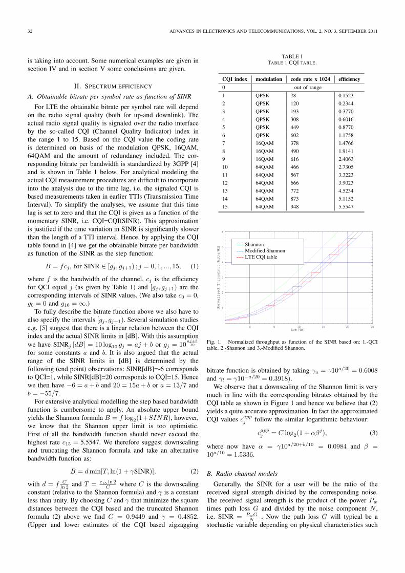
(13)In Figure 2 we have plotted the CDF of the Suzuki dis-

tribution for σ equals 0.2, 0.6, 1.0, 2.0 and 5.0. (The CDFSuzuki distribution is calculated by applying the series (10)with M = 20.0 which secure an accuracy of 2.0x10-9 inthe computation.) Note that the k’th moment of the Suzukidistribution is k! that of the Log-normal.

D. Distribution of the obtainable bitrate for channel of acertain bandwidth for a user located at a given distance fromthe sender antenna

Below we express the distribution of the possible obtainablebitrate according to the distribution of the stochastic part ofthe SINR; namely St. From (1) we get the bit-rate Bt(r) fora channel occupying a bandwidth f located at distance r as:

Bt(r) = fcj when St ∈ [h(r, λ)gj , h(r, λ)gj+1) ,for j = 0, 1, ..., 15. (14)

Hence, the DF (Distribution Function) of the bandwidth distri-bution for a user located at distance r; B(y, r) = P (Bt(r) ≤y) may be written:

B(y, r) = S(h(r, λ)gj+1), for y ∈ (fcj , fcj+1]

for j = 0, 1, ..., 15, (15)

where S(x) is the DF of the variable fading component.Hence, we obtain the k’moment of the obtainable bitrate fora user located at a distance r from the antenna as the (finite)sum:

mk(r) = fk15∑

j=1

(ckj − ckj−1

)S(h(r, λ)gj), (16)

where S(x) = 1 − S(x) is the CDF of the variable fadingcomponent.

Rather than applying the discrete modeling approach abovewe may prefer to apply the smooth (continuous) counterpartdefined by relation (2). The bit-rate Bt(r) for a channeloccupying a bandwidth f located at distance r is then givenby

Bt(r) = dmin[T, ln(1 + St/g(r, λ))], (17)

with d = f Cln 2 and T = c15 ln 2

C and where C is thedownscaling constant (relative to the Shannon formula) andwhere we also define g(r, λ) = γ−1h(r, λ). For the continuousbandwidth case the DF of the bandwidth distribution for a userlocated at distance r is given by:

B(y, r) =

{S(g(r, λ)(ey/d − 1)) for y/d < T1 for y/d ≥ T (18)

Based on (18) we may write the k’moment of the obtainablebitrate for a user located at a distance r from the antenna:

mk(r) = dkg(r,λ)(eT−1)∫

y=0

(ln (1 + y/g(r, λ)))ks(y)dy +

+dkT kS(g(r, λ)(eT − 1) (19)

E. Distribution of the obtainable bitrate for channel of acertain bandwidth for a user that is randomly placed in acircular cell with power-law attenuation

Since the bitrate/capacity for a user will strongly depend ofthe distance from the sender antenna, a better measure of thecapacity will be to find the distribution of bitrate for a user thatis randomly located in the cell. This is done by averaging overthe cell area and therefore the distribution of the correspondingaveraging bitrate Bt is given as B(y) = 1

A

∫AB(y, r)dA(r)

where A is the cell area. For circular cell shape and power lawattenuation on the form h(r, λ) = h(λ)rα (where we also takeg(λ) = γ−1h(λ) i.e. g(r, λ) = g(λ)rα) the correspondingintegral may be partly evaluated. By defining an α-factoraveraging variable Sα with DF Sα(x) = P (Sα ≤ x) givenby

Sα(x) =2

αx−

2α

x∫

t=0

t2α−1S(t)dt =

2

α

1∫

t=0

t2α−1S(tx)dt (20)

and with PDF

sα(x) =2

αx−

2α−1

x∫

t=0

t2α s(t)dt =

2

α

1∫

t=0

t2α s(tx)dt (21)

the bitrate distribution will have the exact same form as (15)for the discrete bandwidth case and (18) for the continuousbandwidth case, and with moments given by (16) and (19) bychanging r → R and S(x)→ Sα(x) (and s(x)→ sα(x)).

1) Distribution of the stochastic variable Sα for Log-normal and Suzuki distribution: Based on the definition wemay derive the CDF and PDF of stochastic variable Sα forthe Log-normal and Suzuki distributed fading models. For theLog-normal distribution we have

Slnα(x) =1

αx2/α

x∫

t=0

t2/α−1erfc

(ln t

σ√2

)dt.


By changing variable according to y = ln t in the integral wefind:

Slnα(x) =1

2

(erfc

(lnx

σ√2

)+

+x−2/αe2σ2/α2

erfc

(2σ2 − α lnx

ασ√2

))(22)

and further the PDF is found by differentiation:

slnα(x) =1

αx−(2/α+1)e2σ

2/α2

erfc

(2σ2 − α lnx

ασ√2

)(23)

For the Suzuki distribution we have the CDF given by theintegral Ssu(x) = x

∫∞t=0

t−2e−tsln(x/t)dt and therefore wehave:

Ssuα(x) =2

α

1∫

t=0

t2/α−1Ssu(xt)dt

= x

∞∫

t=0

t−2e−tslnα(x/t)dt (24)

where slnα(x) is given by (23) above for the Lognormaldistribution. As for the Suzuki distribution approximation toany accuracy is possible to obtain of Ssuα(x) by truncatingthe integral above:

Ssuα(x,M) = x

M∫

t=0


and also for this case we find that the truncation error isexponentially small. By expanding e−t =

∑∞k=0

(−1)ktkk! and

integrating term by term we find:

Ssuα(x,M)=∞∑

k=0

(−1)kxk(2 + kα)k!

ek2σ2

2 erfc

(kσ√2+

ln(x/M)

σ√2

)+

+e2σ

2/α2

αγ

(2

α,M

)x−2/αerfc

(2σ2−α ln(x/M)

ασ√2

)

(26)

where γ(a, x) =∫ xt=0

ta−1e−tdt is the incomplete gammafunction. (Observe the similarity with the corresponding ex-pansion for Ssu(x) by (10).)

The corresponding integral for the PDF is given by:

ssuα(x) =

∞∫

t=0


and we take the truncated approximation of the PDF as theintegral:

ssuα(x,M) =

M∫

t=0


and we find the following error bound: 0 ≤ ssuα(x) −ssuα(x,M) ≤ e−M+σ2

2 . By the similar approach as for the

CDF we find the following series expansion of the truncatedPDF:

ssuα(x,M) =

=∞∑

k=0

(−1)kxk(2+(k+1)α)k!

e(k+1)2σ2

2 erfc

((k+1)σ√

2+ln( xM )

σ√2

)

+e

2σ2

α2

αγ

(2

α+1,M

)x−(1+

2α )erfc

(2σ2−α ln( xM )

ασ√2

)

(29)

III. ESTIMATION OF CELL CAPACITY

In the following we assume that the cell is loaded by twotraffic types:• High priority CBR traffic sources that each requires to

have a fixed data-rate and• Low priority (greedy) data sources that always consumes

the leftover capacity not used by the CBR traffic.This is actually a very realistic traffic scenario for future LTEnetworks where we actual will have a mix of both real timetraffic like VoIP and typical elastic data traffic. Below, wefirst estimate the RB usage of the high priority CBR traffic,and then we may subtract the corresponding RBs to find theactual numbers of RBs available for the (greedy) data trafficsources. Then finally we estimate the cell throughput/capacityas the sum of the bitrates offered to the CBR and (greedy)data sources.

A. Estimation of the capacity usage for GBR sources in LTE

The reservation strategy considered simply allocate re-courses on a per TTI bases and allocate RBs so that theaggregate rate equals the required GBR (Guaranteed Bit Rate)rate (Non-Persistent scheduling).

1) Capacity usage for a single GBR source : We firstconsider the case where we know the location of the CBRuser in the cell, i.e. at a distance r from the antenna. We takeB as the bitrate obtainable for a single RB and consider a GBRsource that requires a fixed bit-rate of bCBR. We assumes thatthis is achieved by offering n RBs for every k-TTI interval.A way of reserving resources to GBR sources is to allocateRBs so that n

kB will be close to the required rate bCBR overa given period. We take NCBR = n

k to be the number ofRBs granted to a GBR connection in a TTI as (the stochasticvariable):

NCBR =

{αbCBR

B if CQI > 00 if CQI = 0

, (30)

where we have introduced a scaling factor α so that on thelong run we obtain the desired GBR-rate bCBR. By choosingα = p−1CQI where pCQI = P (CQI > 0) = S(h(r, λ)g1) thenE [NCBRB] = bCBR and hence we also have:

E [NCBR |CQI > 0 ] =bCBR

pCQIE[B−1 |CQI > 0

]. (31)

The mean numbers of RBs is therefore:

β = β(r, bCBR) = bCBRmCQI−1 (r), (32)


where the conditional moments mCQIk (r) =

E[Bk |CQI > 0

]is found as

mCQIk (r) =

fk

S(h(r, λ)g1)

ck1 S(h(r, λ)g1)+

+15∑

j=2

(ckj − ckj−1

)S(h(r, λ)gj)

, (33)

for the discrete bandwidth case and by

mCQIk (r) =

dk

S(h(r, λ)g1)

g(r,λ)(eT−1)∫

y=h(r,λ)g1

(ln

(1+

y

g(r,λ)

))ks(y)dy+

+T kS(g(r, λ)(eT − 1)

(34)

for the continuous bandwidth case. Note that by conditioningon having CQI > 0 we exclude the users that are unableto communicate due to bad radio conditions and avoid theproblems due to division of zero in the calculation of the meanof 1/B.

For circular cells and power law attenuation we obtain thecorresponding result as above by changing r → R and S(x)→Sα(x).

2) Estimation of RBs usage for several CBR sources: Wefirst estimate the RB usage for a fixed number of M CBRsources located at distances rj from the antenna and with bit-rate requirements bCBRj j = 1, ...,M . The total usage of RBsβCBR will be the sum the individual contribution from eachsource as given by (32):

βCBR =M∑

j=1

β(rj , bCBRj ). (35)

For the case with random location the expression gets evensimpler:

βCBR = β(R,

M∑

j=1

bCBRj ), (36)

i.e. we may add the CBR rates from all the sources in the cell.The corresponding throughput for the CBR sources is takenas the sum of the individual rates i.e.

bCBR =M∑

j=1

bCBRj (37)

B. Estimation of the capacity usage for a fixed number ofgreedy sources

We shall estimate the capacity usage for a fixed number ofgreedy sources under the following assumptions:• There are totally K active (greedy) users that are placed

random in the cell which always have traffic to send, i.e.we consider the cell in saturated conditions.

• There is totally N available RBs and the scheduled useris granted all of them in a TTI interval.

1) Scheduling of based on metrics: In the following weconsider the case with K users that are located in a cell withdistances from the sender antenna given by a distance vectorr = (r1, ...., rK) and we assume that the user scheduled in aTTI is based on:

ischedul = arg maxi=1,..,K

{Mi}, (38)

where Mi = Mi(r) is the scheduling metric which also maydepend on the location of all users (through the location vectorr = (r1, ...., rK)). Hence, for the scheduler to choose user i,the metric Mi must be larger than all the other metrics (forthe other users), i.e. we must have Mi > Ui where

Ui = maxk=1,..,Kk 6=i

Mk. (39)

Since we assume that a user is granted all the RBs whenscheduled, this gives the cell throughput when user is sched-uled (located at distance ri) to be NB(ri), where B(ri) is thecorresponding obtainable bit-rate per RB. Hence, cell bit-ratedistribution (with K users located in the cell with distancevector r = (r1, ...., rK)) may then be written as:

Bg(y, r) =K∑

i=1

Bi(y, r), where (40)

Bi(y, r) = P (NB(ri) ≤ y,Mi(r) > Ui(r)) (41)

is bitrate distribution when user i is scheduled. Unfortunately,for the general case exact expression of the probabilitiesBi(y, r) is difficult to obtain mainly due to the involvement ofthe scheduling metrics. However, for some cases of particularinterest closed form analytical expression is possible to obtain.For many scheduling algorithms the scheduling metrics is onlyfunction of the SINR for that particular user (and does notdepend of the SINR for the other users) and for this caseextensive simplification is possible to obtain. In the followingwe therefore assume that the metrics Mi only are functionsof their own SINRi and the location ri for that particularuser, i.e. we have Mi =M(Si, ri), where we (for simplicity)also assume that M(x, ri) is an increasing function of xwith an unlikely defined inverse M−1(x, ri). The distributionfunctions for Mi and Ui = max

k=1,..,Kk 6=i

Mk are then

Mi(x, ri) = P (Mi ≤ x) = S(M−1(x, ri)) and (42)

Ui(x, r) = P (Ui ≤ x) =K∏

k=1,k 6=iS(M−1(x, rk)) (43)

If we now condition on the value of Si = x in (41), we findthe distribution of the cell capacity when user i is scheduledas:

Bi(y, r) =

∞∫

x=0

P(B(ri) ≤

y

N

∣∣∣Si = x)Ui(M(x, ri), r)s(x)dx.

(44)


By using (14) as the obtainable bit-rate per RB for the discretecase we find:

Bi(y, r) =

h(ri,λ)gj+1∫

x=0

Fi(x, r)s(x)dx, if y/N ∈ (fcj , fcj+1]

for j = 0, 1, ..., 15, (45)

where we now have defined the multiuser “scheduling” func-tion Fi(x, r) by:

Fi(x, r) = Ui(M(x, ri), r) =

K∏

k=1,k 6=iS(M−1(M(x, ri), rk))

(46)Similar for the continuous case based on (17) as the

obtainable bit-rate per RB gives:

Bi(y, r) =

g(ri,λ)(ey/dN−1)∫

x=0

Fi(x, r)s(x)dx for y/dN < T

pi(r) for y/dN ≥ T,

(47)where pi(r) =

∫∞x=0

Fi(x, r)s(x)dx is the probability that useris scheduled in a TTI (and therefore

∑Ki=1 pi(r) = 1).

Finally, by assuming that all users are randomly lo-cated throughout the cell the corresponding bit-rate dis-tribution is found by performing a K-dimensional av-eraging over all possible distance vectors r, over thecell; Bg(y) = 1

AK

∫A. . .∫Ar1 . . . rKBcell(y, r)dA1 · · · dAK ,

where A here is the cell area. Due to the special formof the function Fi(x, r) =

∏Kk=1,k 6=i S(M

−1(M(x, ri), rk))the “cell averaging” over the K − 1 dimension variablesr1, . . . , ri−1, ri+1, . . . , rK (not including the variable ri)

yields the product[_

S(M(x, ri)]K−1

where

_

S(y) =1

A

∫

A

uS(M−1(y, u))dA(u) (48)

Hence, for the case when user i is located at distance riand all the K − 1 other users located at random, then we findfor the discrete case:

Bi(y, ri)=

h(ri,λ)gj+1∫

x=0

[_

S(M(x, ri))]K−1s(x)dx, if y/N ∈ (fcj , fcj+1]

for j = 0, 1, ..., 15 (49)

and for the continuous case:

Bi(y, ri)=

g(ri,λ)(ey/dN−1)∫

x=0

[_

S(M(x, ri))]K−1s(x)dx for y/dN < T

pi(ri) for y/dN ≥ T,(50)

where pi(ri) =∫∞x=0

[_

S(M(x, ri))]K−1

s(x)dx is the proba-bility that user i is scheduled. (Observe that the pi(r) = p(r)and Bi(y, r) = B(y, r) only depend on the location ri andhence are equal for all the users.)

For circular cell size the cell bit-rate distribution integralsabove is reduced to:

Bg(y) =2

R2

R∫

r=0

r

h(r,λ)gj+1∫

x=0

K[_

S(M(x, r))]K−1

s(x)dxdr

if y/N ∈ (fcj , fcj+1] ; for j = 0, 1, ..., 15

(51)

for the discrete case and

Bg(y) =

2R2

R∫r=0

rL(y, r)dr for y/dN < T

1 for y/dN ≥ T(52)

where L(y, r) =∫ g(r,λ)(ey/dN−1)x=0

K[_

S(M(x, r))]K−1

s(x)dx.For the continuous case where we now have

_

S(y) =2

R2

R∫

r=0

uS(M−1(y, u))du (53)

The moments of the capacity (when the users are locatedaccording to the vector r = (r1, ...., rK) may be written as:

E[Bg(r)k] = fkNk

K∑

i=1

15∑

j=1

ckj

h(ri,λ)gj+1∫

x=h(ri,λ)gj

Fi(x, r)s(x)dx (54)

for the discrete bandwidth case and

E[Bg(r)k] =

= dkNkK∑

i=1

g(ri,λ)(e

T−1)∫

x=0

(ln(1+x/g(ri, λ)))kFi(x, r)s(x)dx

+T k∞∫

x=g(ri,λ)(eT−1)

Fi(x, r)s(x)dx

, (55)

for the continuous case.The corresponding moments for the case where the users

are randomly located in a circular cell are given by:

E[Bkg ]=2fkNk

R2

15∑

j=1

ckj

R∫

r=0

r

h(r,λ)gj+1∫

x=h(r,λ)gj

K[_

S(M(x, r))]K−1s(x)dx

dr

(56)for the discrete bandwidth case and

E[Bkg ] =

=2dkNk

R2

R∫

r=0

r

g(r,λ)(eT−1)∫

x=0

(ln

(1 +

x

g(r, λ)

))kL(x, r)s(x)dx

+T k∞∫

x=g(r,λ)(eT−1)

L(x, r)s(x)dx

dr (57)

for the continuous case, where L(x, r) =

K[_

S(M(x, r))]K−1

.


2) Examples: Below we consider and compare three of themost commonly known scheduling algorithms, namely RoundRobin (RR), Proportional Fair (PF) and Max SINR by applyingthe cell capacity models described above.

a) Round Robin : For the Round Robin algorithm eachuser is given the same amount of bandwidth and hence thiscase corresponds to taking K = 1 i.e. the results in section IImay be applied by to find the cell capacity with f → Nf andS(x)→ Ssu(x) and also Sα(x)→ Ssuα(x).

b) Proportional Fair (in SINR) : Normally, the shadow-ing is varying over a much longer time scale than the TTIintervals, and hence we may assume that the slow fading isconstant during the updating of the scheduling metric Mi andtherefore should only account for the rapid fading component.This means that the shadowing effect may be taken as constantthat may be included in the non varying part of the SINRover several TTI intervals. Hence, we take SINR as St/g(r;λ)where St = zXe conditioned that the shadowing Xln = z. Byassuming that Xln = z is constant over the short TTI intervalsthe scheduling metrics will be Mi =

zXe/h(ri,λ)zE[Xe]/h(ri,λ)

= XeE[Xe]

.In the final result we then “integrate over the Log-normalslow fading component”. We find that the probability of beingscheduled is p(r) = 1

K and that the conditional bandwidthdistribution for a user at located at distance r (and the K − 1users random located) is given by the results in section II-Dwith f → Nf and S(x)→ SK(x) with:

SK(x) =

∞∫

t=0

Se

(xt

)Ksln(t)dt and

sK(x) =

∞∫

t=0

K

tSe

(xt

)K−1se

(xt

)sln(t)dt, (58)

where Se(x) = 1− e−x and se(x) = e−x.Further, the distribution of the cell capacity is given by

the results in section II-E with f → Nf and further the α-averaging is given by the integrals:

SKα(x) =

∞∫

t=0

KSe(t)K−1se(t)Slnα

(xt

)dt and (59)

sKα(x) =

∞∫

t=0

KSe(t)K−1se(t)t

−1slnα(xt

)dt (60)

c) Max SINR algorithm.: For this algorithm the schedul-ing metric is Mi = Si/h(ri, λ). By assuming circular cell sizeand radio signal attenuation on the form h(r, λ) = h(λ)rα

gives:

_

S(M(x, r)) =2

R2

R∫

r=0

uS(x(u/r)α)du = Sα(x(R/r)α). (61)

We find that the probability of being scheduled

p(r) =

∞∫

x=0

[Sα(x(R/r)α)]

K−1s(x)dx (62)

and that the conditional bandwidth distribution for a userlocated at distance r (and the K − 1 users random located)is given by the results in section II-D with f → Nf andS(x)→ Sc(x; r) with:

Sc(x; r) =1

p(r)

x∫

y=0

[Sα(y(R/r)α)]

K−1s(y)dx (63)

It turns out that extensive simplifications occur for the casewhere all the users are randomly located in the cell and we findthat the distribution of the cell capacity is given by the resultsin section II-E with f → Nf and further the α-averagingis given by taking Sα(x) → Sα(x)

K i.e. is simply the K’thpower of the α-averaging of S(x).

C. Combining real-time and non real time traffic over LTE

We are now in the position to combine the analysis insections III.A and III.B to obtain complete description of theresource usage in a LTE cell. The combined modeling is basedon the following assumptions:

• There are M CBR sources applying one of the allocationoptions described in section III.A.

• There are totally K active (greedy) data sources whichalways have traffic to send, i.e. we consider the cell insaturated conditions.

• The number of available RBs is taken to be N .

Since the CBR sources have “absolute” priority over the datasources, they will always get the number of RBs they needand hence the leftover RBs will be available for the Non-GBR data sources. By conditioning on the RB usage of theGBR sources we may apply all the results derived in sectionIII.B with available RBs taken to be the leftover RBs not usedby the CBR sources. Then we may find the average usage ofRBs for the CBR traffic as done in section III.A.

We consider first the case where the location of the sourcesis given:

• CBR sources are located at distances sj from the antennawith bit-rate requirements bCBRj ; j = 1, ...,M .

• The greedy data sources are located at distance ri (i =1, ...,K).

With these assumptions the mean cell throughput is givenas:

Bcell =

=f

N−

M∑

j=1

β(sj , bCBRj )

K∑

i=1

15∑

j=1

cj

h(ri,λ)gj+1∫

x=h(ri,λ)gj

Fi(x, r)s(x)dx+

+M∑

j=1

bCBRj , (64)



Bcell =

= d

N −

M∑

j=1

β(sj , bCBRj )

K∑

i=1

Vi(x, r) +

T

∞∫

x=g(ri,λ)(eT−1)

Fi(x, r)s(x)dx

+

M∑

j=1

bCBRj , (65)

for the continuous bandwidth case; where Vi(x, r) =∫ g(ri,λ)(eT−1)x=0

ln(1 + x/g(ri, λ))Fi(x, r)s(x)dx, β(r, bCBR)is given by by (32) and further Fi(x, r) is defined by (46). Forcircular cells and power law attenuation on the form h(r, λ) =h(λ)rα and randomly placed sources the corresponding cellthroughput is found to:

Bcell =

= f

N − β(R,

M∑

j=1

bCBRj )

2

R2

15∑

j=1

cjVj(x, r)

+M∑

j=1

bCBRj (66)

where

Vj(x, r) =

R∫

r=0

r

h(r,λ)gj+1∫

x=h(r,λ)gj

K[_

S(M(x, r))]K−1

s(x)dx

dr


Bcell =

= d(N − β(R,M∑

j=1

bCBRj ))2

R2

R∫

r=0

r

V (x, r)

+T

∞∫

x=g(r,λ)(eT−1)

K[_

S(M(x, r))]K−1s(x)dx

dr +

M∑

j=1

bCBRj

(67)

for the continuous bandwidth case; where V (x, r) =∫ g(r,λ)(eT−1)x=0

ln(1 + x/g(r, λ))K[_

S(M(x, r))]K−1

s(x)dx,

β = β(r, bCBR) is given by (32) and further_

S(M(x, r)) isdefined by (53). Observe that the CBR traffic only will affectthe cell throughput by the sum

∑Mj=1 b

CBRj of the rates and

not the actual number of CBR sources.

IV. DISCUSSION OF NUMERICAL EXAMPLES

In the following we give some numerical example ofdownlink performance of LTE. Before describing the resultswe first rephrase some of the main assumptions:• The fading model includes lognormal shadowing (slow

fading) and Rayleigh fast fading.• The noise interference is assumed to be constant over the

cell area.

TABLE IIINPUT PARAMETERS FOR THE NUMERICAL CALCULATIONS

Parameters Numerical values

Bandwidth per Resource Block 180 kHz=12x 15 kHzTotal Numbers of Resource Blocks(RB)

100 RBs for 2Ghz

Distance-dependent path loss. (Theactual model is found in [4].)

L = C + 37.6 log10(r),r in kilometers andC=128.1 dB for 2GHz,

Lognormal Shadowing with stan-dard deviation

8 dB (in moust of the cases)

Rayleigh fast fadingNoise power at the receiver -101 dBmTotal send power 46.0 dBm=(40W)Radio signaling overhead 3/14

• The cell shape is circular.Basically, there are three different cases we would like toinvestigate. First and foremost is of course the actual efficiencyof the LTE radio interface. We choose the bitrate obtainable forthe smallest unit available for users, namely a Resource Block(RB). Since different implementation may chose differentbandwidth configurations the performance based on RBs willgive a good indication of the overall capacity/throughputfor the LTE radio interface. Secondly, we know that thescheduling also will affect the overall throughput for a LTEcell. Based on the modeling we are able to investigate theperformance of the three basic scheduling algorithms: RoundRobin (RR), Proportional Fair (PF) and Max-SINR. All thesethree algorithms have their weaknesses and strengths, likeMax-SINR that try to maximize the throughput but at the costof fairness among users. Thirdly, we would also investigatethe effect on overall performance by introducing GBR trafficin LTE. Normally, GBR traffic will higher priority than Non-GBR or “best effort” traffic and to guarantee a particular ratethe number of radio resources required may vary dependingon the radio conditions. For users with bad radio conditionsi.e. located at cell edge the resource usage to maintain afixed guaranteed rate may be quite high so an investigationof the cell performance with both GBR and Non-GBR will beimportant.

A. LTE spectrum efficiency

First, we consider bitrate that is possible to obtainable forthe basic resource unit in LTE namely a RB. In the exampleswe have considered sending frequency of 2 GHz. The aim isto predict the bandwidth efficiency, i.e. the obtainable bitrateper RB. The rest of the input parameters are given in Table 2.

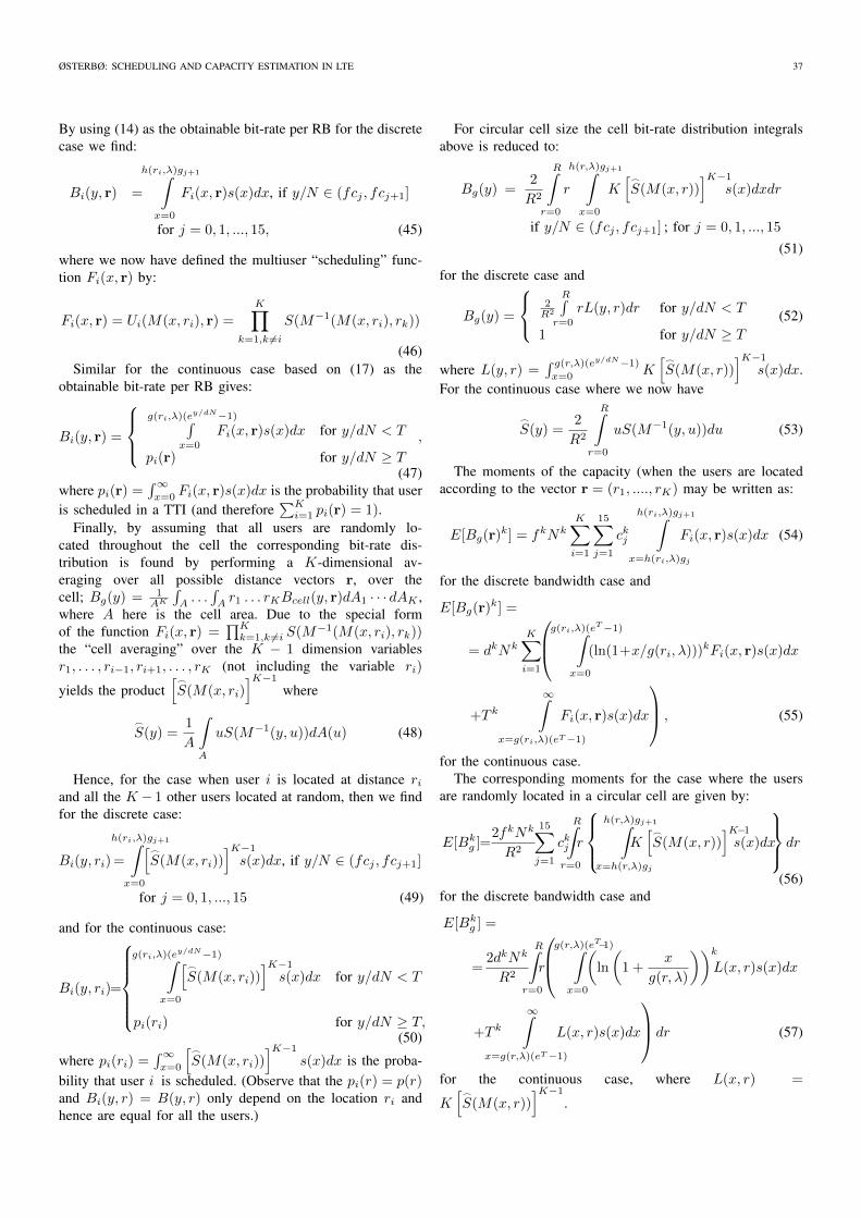
The mean obtainable bitrate per RB is depicted in Figure3. With our assumptions the maximum bitrate is just below0.8 Mbit/s for excellent radio conditions. The mean bit-rate isas expected a decreasing function of the cell size both for arandomly placed user and for a user at the cell edge. The meanbitrate have decreased to 0.1 Mbit/s per RB for cell sizes ofapproximately 2 km for shadowing std. equals 8 dB and whenusers are random located. The corresponding bit-rate for usersat the cell edge is proximately 0.04 Mbit/s.


1 2 3 4 5Distance @KmD

0.1

0.2

0.3

0.4

0.5

0.6

0.7

0.8

na

eM

tu

ph

gu

or

ht

rep

BR

@t

ibM

êsD

Located at cell

edge

Random

location

Fig. 3. Mean throughput right and std. left per RB for a user random located,and fixed located as function of cell radius with 2 GHz sending frequency andSuzuki distributed fading with std. of fading σ=0dB, 2dB, 5dB, 8dB, 12dBfrom below.

B. Cell capacity and scheduling

Below we examine the downlink performance in an LTE cellwith the input parameters given by Table 2, however, with thefollowing additional input parameters:• Type of scheduling algorithm i.e. RR, PF or Max-SINR,• number of RB available i.e. 100,• number of active (greedy) users.

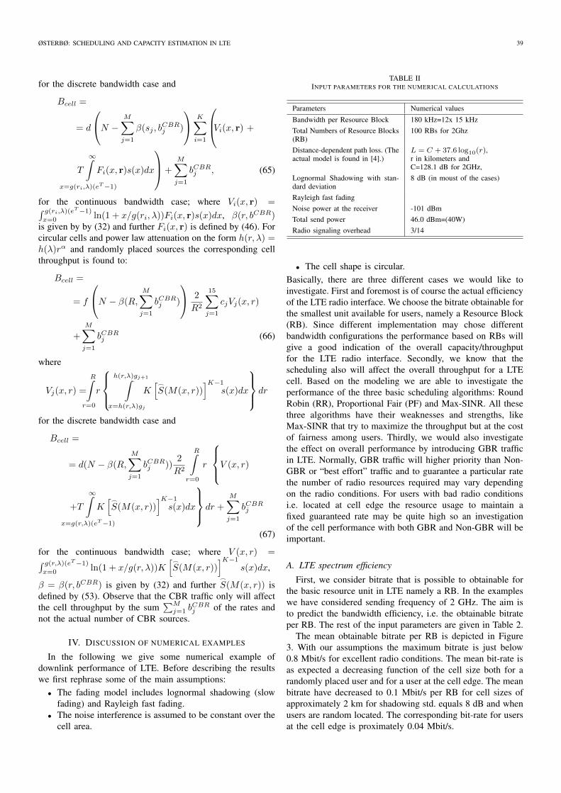
In Figure 4 the mean downlink cell capacity is depictedas function of the cell radius for RR, PF and the MaxSINR scheduling algorithms. As expected the Round Robinalgorithm gives the lowest cell throughput while the MaxSINR algorithm give the highest throughput. For the latterthe multiuser gain is huge and may be explained from thefact that when the number of users increases those who bychance are located near the sender antenna will with highprobability obtain the best radio condition and will therefore bescheduled with high bit-rate. For users located at the cell edgethe situation is opposite and those users will normally have lowSINR and surely obtain very little of the shared capacity. Thisexplains why the Max SINR will increase the throughput butis highly un-fair. For the PF only the relative size of the SINRis important and in this case each user has equal probabilityof sending in each TTI. The multiuser gain for this algorithmis much lower than for the Max SINR algorithm but is notnegligible. When it comes to actual cell downlink throughputthe expected values lays in the range 26-48 Mbit/s for cellswith radius of 1 km while if the radius is increased to 2 kmthe cell throughput is reduced to approximately 10-20 Mbit/s.

As seen from Figure 4 the Max-SINR algorithm will overperform the PF algorithm when it comes to cell throughput.But if we consider fairness among users the picture is completedifferent. When considering the performance of users locatedat cell edge the Max-SINR algorithm actually performs verybadly. While PF give equal probability of transmitting in aTTI for all active users the Max-SINR strongly discriminatethe user close to cell edge. As seen from Table 3 below; if thereare totally 10 active users in a cell the PF fairly give each user10% chance of accessing radio resource while the Max-SINR

1 2 3 4 5Distance @KmD

10

20

30

40

50

60

70

80

ll

eC

yt

ic

ap

ac

@t

ib

MêsD

-- PF

-- Max-SINR

-- RR

Fig. 4. Multiuser gain as function of cell radius for Max-SINR (red), PF(blue) and RR (black) scheduling, 2GMHz frequency with 100 RB and withSuzuki distributed fading with std. σ = 8 dB. The number of users is 1, 2,3, 5, 10, 25, 100 from below.

TABLE IIIPROBABILITY THAT A USER IS SCHEDULED AS FUNCTION OF NUMBERS OF

USERS AND LOCATION FOR PF AND MAX-SINR SCHEDULINGALGORITHMS, SUZUKI DISTRIBUTED FADING WITH STD. OF 8DB.

Number of users PF MAX-SINR

r/R=1 r/R=0.5 r/R=0.25 r/R=0.12 0.50 0.308708 0.594756 0.82579 0.961193 0.33 0.147869 0.414839 0.71126 0.927845 0.20 0.055113 0.245871 0.56102 0.8713010 0.10 0.012690 0.104912 0.36531 0.7641825 0.04 0.001356 0.025222 0.16326 0.56989

100 0.01 0.000019 0.001293 0.02453 0.24325

only give 1.2% chance of accessing the radio resources if auser is located at cell edge. As the number of user increasesthis unfairness increases even more.

Table 3 demonstrates one of the unfortunate properties ofthe MAX-SINR scheduling algorithm. While the PF algorithmdistribute the capacity among the users with equal probabilitythe MAX-SINR algorithm is far more unfair when it comes tothe distribution of the available radio resources. For instance,the users located at the cell edge e.g. r/R=1 will suffer fromextremely poor performance if the numbers of users is higherthan 10. The Max-SINR algorithm will also be unfair forsmall cell sizes where users actually may have so high signalquality that most of them may use coding with high data ratei.e. 64 QAM with high rare and there should be no need forscheduling according highest SINR to obtain high throughput.

C. Use of GBR in LTE

It is likely the LTE in the future will carry both real timetype traffic like VoIP and elastic data traffic. This is possibleby introducing GBR bearers where users are guaranteed thepossibility to send at their defined GBR rate. The GBR trafficwill have priority over the Non-GBR traffic such that the RBsscheduled for GBR bearers will normally not be accessiblefor other type of traffic. However, the resource usage overthe radio interface in LTE will strongly depends on the radio


conditions. This means that the amount of radio resources auser occupies (to obtain a certain bit rate) will vary accordingto the local radio conditions and a user at the cell edge mustseize a larger number of resource blocks (RBs) to maintain aconstant rate (GBR bearer) than a user located near the antennawith good radio signals.

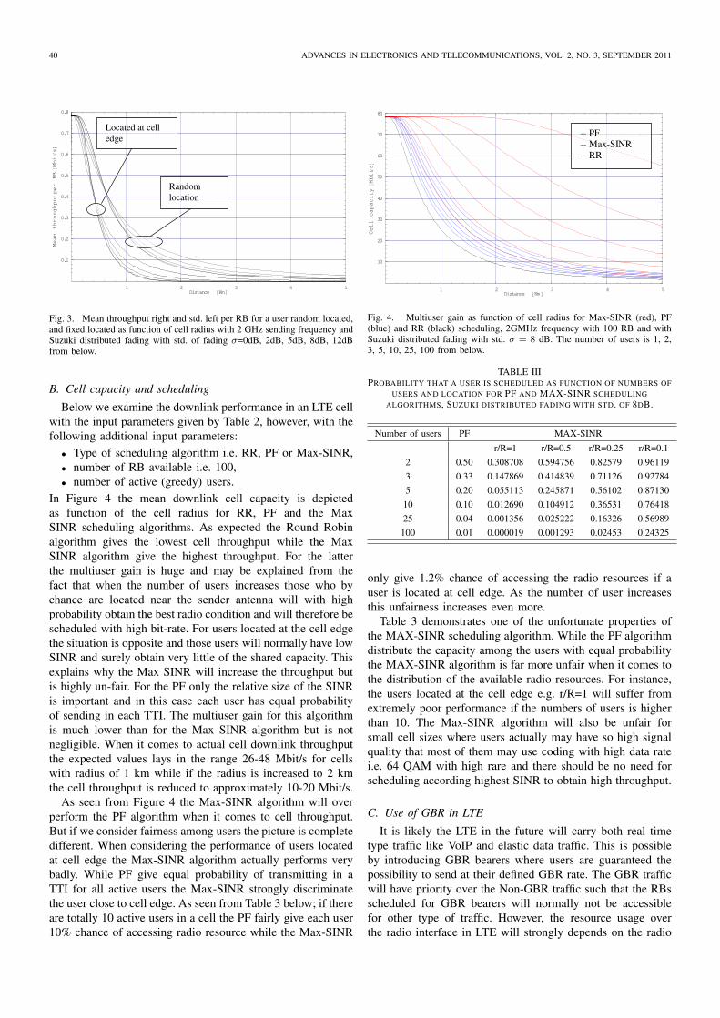
An interesting example is to see the effect of multiplexingtraffic with both greedy and GBR users and observe the effecton the cell throughput. In Figure 5 we consider the cases where10 greedy users are scheduled by the PF algorithm togetherwith a GBR user with guaranteed rate of 3, 1, 0.3 or 0.1 Mbit/s.We consider the cases where either the GBR user is locatedat cell edge or have random location throughout the cell.

We observe that thin GBR connections do not have bigimpact on the cell throughput. From the figures it seems thatGBR bearers up to 1 Mbit/s should be manageable withoutinfluencing the cell performance very much. But a 3 Mbit/sGBR connection will lower the total throughput by a quite bigfactor especially if the user is located at cell edge. For instancewe observe for both cases that the effective reduction in cellthroughput is approximately 20 Mbit/s for a user requiring a3 Mbit/s GBR connection when located at cell edge. As aconsequence we recommend limiting GBR connection to lessthan 1 Mbit/s.

We therefore recommend using high GBR values withparticular caution. The GBR should be limited to a maximumrate to avoid that a particular GBR user consumes a too largepart of the radio resources (too many RBs). A good choice ofthe actual maximum GBR value seems to be around 1 Mbit/s.

V. CONCLUSIONS

With the introduction of LTE the capacity in the radionetwork will increase considerably. This is mainly due to theefficient and sophisticated coding methods developed duringthe last decade. However, the cost of such efficiency is thatthe variation due to radio conditions will increase significantlyand hence the possible capacity for users in terms of bitratewill vary a lot depending on the current radio conditions.

The two most important factors for the radio conditions arefading and attenuation due to distance. By extensive analyticalmodeling where both fading and the attenuation due thedistance are included we obtain performance models for:• Spectrum efficiency through the bitrate distribution per

RB for customers that are either randomly or located ata particular distance in a cell.

• Cell throughput/capacity and fairness by taking thescheduling into account.

• Specific models for the three basic types of schedulingalgorithms; Round Robin, Proportional Fair and MaxSINR.

• Cell throughput/capacity for a mix of GBR and Non-GBR(greedy) users.

Numerical examples for LTE downlink show results which arereasonable; in the range 25-50 Mbit/s for 1 km cell radius at2GHz with 100 RBs. The multiuser gain is large for the Max-SINR algorithm but also the Proportional Fair algorithm givesrelative large gain relative to plain Round Robin. The Max-SINR has the weakness that it is highly unfair in its behaviour.

0.5 1 1.5 2 2.5Distance @KmD

10

20

30

40

50

60

70

80

ll

eC

yt

ic

ap

ac

@t

ib

MêsD

0.5 1 1.5 2 2.5Distance @KmD

10

20

30

40

50

60

70

80

ll

eC

yt

ic

ap

ac

@t

ib

MêsD

0.5 1 1.5 2 2.5Distance @KmD

10

20

30

40

50

60

70

80

lle

Cyt

ica

pa

c@

ti

bM

êsD

0.5 1 1.5 2 2.5Distance @KmD

10

20

30

40

50

60

70

80

ll

eC

yt

ic

ap

ac

@t

ib

MêsD

-- Non-Persistent, cell edge

-- Non-Persistent, random

-- mean PF 10 users

GBR=1 Mbit/s

GBR=0.3 Mbit/s



-- mean PF 10 users

GBR=0.1 Mbit/s



-- mean PF 10 users

GBR=3 Mbit/s



-- mean PF 10 users

Fig. 5. Mean cell throughput for PF, 10 users and a GBR user of 3.0,1.0, 0.3, 0.1 Mbit/s using non-persistent scheduling, for 2 GHz and 100 RBand Suzuki distributed fading with std. σ = 8dB. Red curves corresponds torandom location and blue for user located at cell edge.


User at cell edge with poor radio condition will obtain verylittle data throughput. It turns out that the grade of unfairnessincreases with the numbers of active users. This unfortunateproperty is not found for the Proportional Fairs schedulingalgorithm.

The usage of GBR with high rates may cause problems inLTE due to the high demand for radio resources if users havelow SINR i.e. at cell edge. For non-persistent GBR allocationthe allowed guaranteed rate should be limited. It seems that alimit close to 1 Mbit/s will be a good choice.

REFERENCES

[1] H. Holma and A. Toskala, LTE for UMTS, OFDMA and SC-FDMA BasedRadio Access. Wiley, 2009.

[2] R.-. 3GPP TSG-RAN1#48, “LTE physical layer framework for perfor-mance verification,” 3GPP, St. Louis, MI, USA, Tech. Rep., Feb. 2007.

[3] H. Kushner and P. Whiting, “Asymptotic Properties of Proportional-Fair Sharing Algorithms,” in Proc. of 2002 Allerton Conference onCommunication, Control and Computing, Oct. 2002.

[4] 3GPP TS 36.213 V9.2.0, “Physical layer procedures, Table 7.2.3-1: 4-bitCQI Table,” 3GPP, Tech. Rep., Jun. 2010.

[5] M. C, M. Wrulich, J. C. Ikuno, D. Bosanska, and M. Rupp, “Simulatingthe Long Term Evolution Physical Layer,” in Proc. of 17th EuropeanSignal Processing Conference (EUSIPCO 2009), Glasgow, Scotland, Aug.2009.

[6] B. Sklar, “Rayleigh Fading Channels in Mobile Digital CommunicationSystems Part I: Characterization and Part II: Mitigation,” IEEE Commun.Mag., Jul. 1997.

Olav N. Østerbø received his MSc in Applied Mathematics from theUniversity of Bergen in 1980 and his PhD from the Norwegian Universityof Science and Technology in 2004. He joined Telenor in 1980. His maininterests include teletraffic modeling and performance analysis of variousaspects of telecom networks. Activities in recent years have been relatedto dimensioning and performance analysis of IP networks, where the mainfocus is on modeling and control of different parts of next generation IP-based networks.

Documents

Scheduling and Capacity Estimation in · PDF fileScheduling and Capacity Estimation in LTE ... we estimate the total cell throughput/capacity by taking the ... modulation for uplink