Embed Size (px)
DESCRIPTION
Capacity estimation methods applied to mini hydro plants
Citation preview

Capacity Estimation Methods Applied to Mini Hydro Plants 311
Capacity Estimation Methods Applied to Mini Hydro Plants
Rafael Peña and Aurelio Medina
X
Capacity Estimation Methods Applied to Mini Hydro Plants
Rafael Peña and Aurelio Medina
Universidad Michoacana de San Nicolás de Hidalgo México
1. Introduction
Mini hydro generation is one of the most cost-effective and reliable energy technologies in distributed generation systems to be considered for providing clean electricity generation. These systems constitute a viable alternative to address generation and electric power supply problems to isolated regions or small loads. In particular, the key advantages that small hydro has over other technologies considered in distributed generation systems, such as, wind, wave and solar power are (BHA, 2005):
A high efficiency (70 - 90%), by far the best of all energy technologies. A high capacity factor (typically >50%), compared with 10% for solar and 30% for
wind. A high level of predictability, varying with annual rainfall patterns. Slow rate of change; the output power varies only gradually from day to day (not
from minute to minute). It is a long-lasting and robust technology; systems can readily be engineered to last
for 30 years or more.
It is also environmentally benign. Small hydro is in most cases “run-of-river”; in other words any dam or barrage is quite small, usually just a weir, and little or no water is stored. Therefore run-of-river installations do not have the same kind of adverse effects on the local environment as large-scale hydro plants. There is no consensus on the definition of mini hydro plants. Some countries like Portugal, Spain, Ireland, and now, Greece and Belgium, accept 10 MW as the upper limit for installed capacity. In Italy the limit is fixed at 3 MW (plants with larger installed power should sell their electricity at lower prices); in France the limit was established at 8 MW and UK favours 5 MW. Hereunder will be considered as Mini Hydro any scheme with an installed capacity of 10 MW or less. Today, among all the renewable energies, hydropower occupies the first place in the world and it will keep this place for many years to come. Figure 1 shows the electricity generation from renewable energies; it can be seen that the hydro generation represents the 94.3% of the total of the generation using renewable resources; from this percentage, the 9.3% is generated by mini hydro plants. Also, the market for small power plants is more attractive
14

Distributed Generation 312
than ever, due to the power market liberalization in the world, which opens the opportunity for the industry to generate electricity to full fill its basic needs.
Fig. 1. Electricity generation from renewable energy (BHA, 2005) An important aspect on this type of systems is the planning, design and evaluation of the potential energy available in a selected place (Puttgen et al., 2003). The best geographical areas for mini hydro plants are those where there are steep rivers, streams, creeks or springs flowing year-round, such as in hilly areas with high year-round rainfall. To assess the suitability of a site for a mini hydro power system, a feasibility study should be made. Feasibility studies show how the water flow varies along the years and where the water should be taken to obtain its maximum profit; they also show the power amount that can be obtained from the water flow, as well as the minimum and maximum limits of the profitable power. There are other important factors that should be addressed when deciding if a mini hydro plant would work at a specific site:
The potential for hydropower at the site. The requirements for energy and power. Environmental impact and approvals. Equipment options. Costs and economics.
Keep in mind that each micro-hydropower system cost, approvals, layout and other factors are site-specific and unique for each case. In the literature concerning the design and selection of the main components of a mini hydro plant (Penche, 1998; Khennas et al., 2000; ITDG, 1996), the size of the generator is chosen based on the water flow time series organized into a relative frequency histogram, and with a pre-selected plant factor, whose value usually varies from 0.70 to 0.85 for this type of systems (ITDG, 1996). From this information, it is also possible to calculate the theoretical average power and the average annual generation that can be obtained from the site (e.g. river). In this chapter, forecast methodologies based on data measurements from a monthly water flow time series are applied to predict the behaviour of the water for a particular river where it is desired to install the mini hydro plant. First, forecast techniques are discussed and then a example of the application of the techniques to the water flow time series is presented. The proposed procedure aims enhancing the estimation of the generator capacity as the historical data of water flow is now complemented with the results obtained via
forecast techniques (Peña et al., 2009). For completeness, a selection of the most important electro-mechanical elements of a proposed mini hydro plant is also provided.
2. Water Flow Time Series
In order to determine the hydro potential of water flowing from the river or stream, it is necessary to know the flow rate of the water and the head through which the water can fall. The flow rate is the quantity of water flowing past a point at a given time. Typical units used for flow rate are cubic metres per second (m3/s), litres per second (lps), gallons per minute (gpm) and cubic feet per minute (cfm). The head is the vertical height in metres (m) or feet (ft.) from the level where the water enters the intake pipe (penstock) to the level where the water leaves the turbine housing. The measurements or historical data of water flow can be organized into a water flow time series. A time series is a series of measurements, observations, and recordings of a set of variables at successive points in uniform time intervals (Hamilton, 1994). Fig. 2 shows the water flow time series used in this chapter. This historical data corresponds to measurements taken from the Cardel Hydrometric Station, in La Antigua River, Veracruz, México. The time series has 420 monthly observations, from the period of January, 1951 to December, 1985 (CONAE, 2005).
0
100
200
300
400
500
600
700
800
900
1 51 101 151 201 251 301 351 401
Wat
er F
low
(m3 )
Historical Data
1 x 10⁵
Fig. 2. Water flow time series
3. Capacity Estimation: Classic Method
Records of water flow variations along the years are taken in hydrometric stations located in the main rivers. These stations take data about the hydrologic situation of the area including the water flow variations of the river; this is periodically measured, in some cases on a day-to-day basis. The water flow records are very useful to allow forecasting the future behaviour of the river. This data is also taken into account to decide if a mini hydro plant can be installed in a specific place.

Capacity Estimation Methods Applied to Mini Hydro Plants 313
than ever, due to the power market liberalization in the world, which opens the opportunity for the industry to generate electricity to full fill its basic needs.
Fig. 1. Electricity generation from renewable energy (BHA, 2005) An important aspect on this type of systems is the planning, design and evaluation of the potential energy available in a selected place (Puttgen et al., 2003). The best geographical areas for mini hydro plants are those where there are steep rivers, streams, creeks or springs flowing year-round, such as in hilly areas with high year-round rainfall. To assess the suitability of a site for a mini hydro power system, a feasibility study should be made. Feasibility studies show how the water flow varies along the years and where the water should be taken to obtain its maximum profit; they also show the power amount that can be obtained from the water flow, as well as the minimum and maximum limits of the profitable power. There are other important factors that should be addressed when deciding if a mini hydro plant would work at a specific site:
The potential for hydropower at the site. The requirements for energy and power. Environmental impact and approvals. Equipment options. Costs and economics.
Keep in mind that each micro-hydropower system cost, approvals, layout and other factors are site-specific and unique for each case. In the literature concerning the design and selection of the main components of a mini hydro plant (Penche, 1998; Khennas et al., 2000; ITDG, 1996), the size of the generator is chosen based on the water flow time series organized into a relative frequency histogram, and with a pre-selected plant factor, whose value usually varies from 0.70 to 0.85 for this type of systems (ITDG, 1996). From this information, it is also possible to calculate the theoretical average power and the average annual generation that can be obtained from the site (e.g. river). In this chapter, forecast methodologies based on data measurements from a monthly water flow time series are applied to predict the behaviour of the water for a particular river where it is desired to install the mini hydro plant. First, forecast techniques are discussed and then a example of the application of the techniques to the water flow time series is presented. The proposed procedure aims enhancing the estimation of the generator capacity as the historical data of water flow is now complemented with the results obtained via
forecast techniques (Peña et al., 2009). For completeness, a selection of the most important electro-mechanical elements of a proposed mini hydro plant is also provided.
2. Water Flow Time Series
In order to determine the hydro potential of water flowing from the river or stream, it is necessary to know the flow rate of the water and the head through which the water can fall. The flow rate is the quantity of water flowing past a point at a given time. Typical units used for flow rate are cubic metres per second (m3/s), litres per second (lps), gallons per minute (gpm) and cubic feet per minute (cfm). The head is the vertical height in metres (m) or feet (ft.) from the level where the water enters the intake pipe (penstock) to the level where the water leaves the turbine housing. The measurements or historical data of water flow can be organized into a water flow time series. A time series is a series of measurements, observations, and recordings of a set of variables at successive points in uniform time intervals (Hamilton, 1994). Fig. 2 shows the water flow time series used in this chapter. This historical data corresponds to measurements taken from the Cardel Hydrometric Station, in La Antigua River, Veracruz, México. The time series has 420 monthly observations, from the period of January, 1951 to December, 1985 (CONAE, 2005).
0
100
200
300
400
500
600
700
800
900
1 51 101 151 201 251 301 351 401
Wat
er F
low
(m3 )
Historical Data
1 x 10⁵
Fig. 2. Water flow time series
3. Capacity Estimation: Classic Method
Records of water flow variations along the years are taken in hydrometric stations located in the main rivers. These stations take data about the hydrologic situation of the area including the water flow variations of the river; this is periodically measured, in some cases on a day-to-day basis. The water flow records are very useful to allow forecasting the future behaviour of the river. This data is also taken into account to decide if a mini hydro plant can be installed in a specific place.

Distributed Generation 314
From historical records of water flow, a Flow Duration Curve (FDC) can be built. The flow duration curve is a plot that shows the percentage of time that the water flow in a river is likely to equal or exceed a specified value of interest (the area below the curve is a measure of the potential energy of the river or stream). For instance, the FDC can be used to assess the expected availability of water flow over time and the power and energy at a site and to decide on the “design flow” in order to select the turbine. Decisions can also be made on how large a generating unit should be. If a system is to be independent of any other energy or utility backup, the design flow should be the flow that is available 70% of the time or more. Therefore, a stand-alone system such as a mini hydro plant should be designed according to the flow available throughout the year; this is usually the flow during the dry season. It is possible that some streams could dry up completely at that time. Figure 3 shows the FDC for the time series under study. From this figure it is possible to observe that for nearly 80% of the time the water flow is equal or below to 28.4 105 m3. Also, it shows that if a mini hydro plant is to be installed in this river and it is desirable to have it working 70% of the time, then a value of 42.28 105 m3 should be chosen as the design water flow.
0
100
200
300
400
500
600
700
800
900
0.24 12.14 24.05 35.95 47.86 59.76 71.67 83.57 95.48
Wat
er F
low
(m3 )
Historical Data
1 x 10⁵
Time (%) Fig. 3. Flow duration curve Another important graph derived from the historical data is the relative frequency histogram. The relative frequency is defined as the number of times that a value occurs in a data set. Figure 4 shows the relative frequency histogram calculated from the historical data under study. From this bar chart it is possible to a priori visualize the data concentration, and the minimum and maximum values of the time series, e.g. from Figure 4, it can be seen that the value with more repetitions in the time series is 24.2 105 m3.
0.00
0.05
0.10
0.15
0.20
0.25
0.30
0.35
Rel
ativ
e Fre
quen
cy
Water Flow (m3)
1 x 10⁵
Fig. 4. Relative frequency histogram
4. Forecast Techniques
As mentioned before the water flow time series is frequently used for the design and capacity estimation of mini hydro plants. However, records of these variables from a previously selected place are not always available or there is just a few historical data. Besides, climate changes around the world have provoked, for instance, that drought and rainy seasons are not as periodic as they used to be; this makes the water flow levels to change drastically from one season to another, and in some cases rivers even tend to dry-out. The reasons given before and other unexpected events justify the application of forecast techniques to appropriately process the available hydro resources at a specific geographic site, so that an adequate capacity estimation of a mini hydro plant can be achieved (and also to know the future behaviour of a selected river). In order to deal with the forecast problem, various forecast techniques have been used: Kalman Filters (Sorensen & Madsen, 2003), Box-Jenkins methodologies (Montañés et al., 2002), Neural Networks (Xie et al., 2006), etc. most of them providing satisfactory results. In this chapter, ARIMA (Zhou et al., 2004), Neural Networks (Azadeh et al., 2007), and Genetic Programming (Flores et al., 2005) methodologies are presented and then applied to the water flow time series to forecast the behaviour of the water flow in the years to come. The best forecast obtained with the application of these methods is then used to estimate the capacity of a proposed mini hydro plant.
4.1 ARIMA Model The acronym ARIMA stands for “Auto-Regressive Integrated Moving Average”, whose model is a generalization of an auto-regressive moving average or ARMA model. These models are widely used in the time series forecast problem and they are usually part of the Box-Jenkins methodology (Montañés et al., 2002). The ARIMA model is generally referred as an ARIMA(p, d, q) model, where p, d, and q are values used to define the number of auto-regressive, integrated, and moving average terms of the model, respectively.

Capacity Estimation Methods Applied to Mini Hydro Plants 315
From historical records of water flow, a Flow Duration Curve (FDC) can be built. The flow duration curve is a plot that shows the percentage of time that the water flow in a river is likely to equal or exceed a specified value of interest (the area below the curve is a measure of the potential energy of the river or stream). For instance, the FDC can be used to assess the expected availability of water flow over time and the power and energy at a site and to decide on the “design flow” in order to select the turbine. Decisions can also be made on how large a generating unit should be. If a system is to be independent of any other energy or utility backup, the design flow should be the flow that is available 70% of the time or more. Therefore, a stand-alone system such as a mini hydro plant should be designed according to the flow available throughout the year; this is usually the flow during the dry season. It is possible that some streams could dry up completely at that time. Figure 3 shows the FDC for the time series under study. From this figure it is possible to observe that for nearly 80% of the time the water flow is equal or below to 28.4 105 m3. Also, it shows that if a mini hydro plant is to be installed in this river and it is desirable to have it working 70% of the time, then a value of 42.28 105 m3 should be chosen as the design water flow.
0
100
200
300
400
500
600
700
800
900
0.24 12.14 24.05 35.95 47.86 59.76 71.67 83.57 95.48
Wat
er F
low
(m3 )
Historical Data
1 x 10⁵
Time (%) Fig. 3. Flow duration curve Another important graph derived from the historical data is the relative frequency histogram. The relative frequency is defined as the number of times that a value occurs in a data set. Figure 4 shows the relative frequency histogram calculated from the historical data under study. From this bar chart it is possible to a priori visualize the data concentration, and the minimum and maximum values of the time series, e.g. from Figure 4, it can be seen that the value with more repetitions in the time series is 24.2 105 m3.
0.00
0.05
0.10
0.15
0.20
0.25
0.30
0.35
Rel
ativ
e Fre
quen
cy
Water Flow (m3)
1 x 10⁵
Fig. 4. Relative frequency histogram
4. Forecast Techniques
As mentioned before the water flow time series is frequently used for the design and capacity estimation of mini hydro plants. However, records of these variables from a previously selected place are not always available or there is just a few historical data. Besides, climate changes around the world have provoked, for instance, that drought and rainy seasons are not as periodic as they used to be; this makes the water flow levels to change drastically from one season to another, and in some cases rivers even tend to dry-out. The reasons given before and other unexpected events justify the application of forecast techniques to appropriately process the available hydro resources at a specific geographic site, so that an adequate capacity estimation of a mini hydro plant can be achieved (and also to know the future behaviour of a selected river). In order to deal with the forecast problem, various forecast techniques have been used: Kalman Filters (Sorensen & Madsen, 2003), Box-Jenkins methodologies (Montañés et al., 2002), Neural Networks (Xie et al., 2006), etc. most of them providing satisfactory results. In this chapter, ARIMA (Zhou et al., 2004), Neural Networks (Azadeh et al., 2007), and Genetic Programming (Flores et al., 2005) methodologies are presented and then applied to the water flow time series to forecast the behaviour of the water flow in the years to come. The best forecast obtained with the application of these methods is then used to estimate the capacity of a proposed mini hydro plant.
4.1 ARIMA Model The acronym ARIMA stands for “Auto-Regressive Integrated Moving Average”, whose model is a generalization of an auto-regressive moving average or ARMA model. These models are widely used in the time series forecast problem and they are usually part of the Box-Jenkins methodology (Montañés et al., 2002). The ARIMA model is generally referred as an ARIMA(p, d, q) model, where p, d, and q are values used to define the number of auto-regressive, integrated, and moving average terms of the model, respectively.

Distributed Generation 316
In order to describe the mathematics involved in an ARIMA model, it is important to define an ARMA(p, q) model for a data time series X(n), where n is an integer index to indicate a specific data within the time series, then an ARMA(p, q) model is given by (Ramachandran & Bhethanabotla, 2000)
(1-1
p
i i Li) X(n) = (1+
1
q
i θi Li) n (1)
where L is the lag operator, i are the auto-regressive parameters of the model, θi are the moving average parameters of the model, and n are error terms. The error terms n are usually known as white noise and they are assumed to be independent with zero co-variances, and identically distributed sampled data from a normal distribution with zero average. The ARIMA(p, d, q) model can be obtained integrating Equation (1). That is,
(1-1
p
i i Li ) (1-L)d X(n) = (1+
1
q
i θi Li) n (2)
where d is a positive integer that controls the level of differentiation. Note that if d = 0, this model is equivalent to an ARMA model. There are three basic steps to the development of an ARIMA model (Brockwell & Davis, 2002):
1) Identification/model selection: the values of p, d, and q must be determined. The principle of parsimony, also known as principle of simplicity, is adopted; most stationary time series can be modeled using very low values of p and q.
2) Estimation: the θ and the parameters must be estimated, usually by employing a least squares approximation to the maximum likelihood estimator.
3) Diagnostic checking: the estimated model must be checked for its adequacy and revised if necessary, implying that this entire process may have to be repeated until a satisfactory model is found.
The most crucial of these steps is identification, or model selection. This step requires the researcher to use his or her personal judgment to interpret some selected statistics, in conjunction with a graph from a set of autocorrelation coefficients, to determine which model the data suggest is the appropriate one to be employed. In this respect the ARIMA model is an art form, requiring considerable experience for a researcher to able to select the correct model. Using the R-Project software (R-Project, 2009), a model that allows the determination of each ARIMA parameters was implemented; 370 data points were used to obtain the model and the last 50 values of the time series were used to compare the forecast obtained by the model with the results from the historical time series. For an ARIMA (3, 1, 2) model, e.g. with three auto-regressive parameters (ARX), one integrator parameter (INTGX) and two moving average parameters (MAX), the coefficients shown in Table 1 were obtained.
AR1 AR2 AR3 MA1 MA2 INTG1 -0.1559 0.2239 0.0753 -0.5109 -0.4891 -0.4652
Table 1. ARIMA technique coefficients
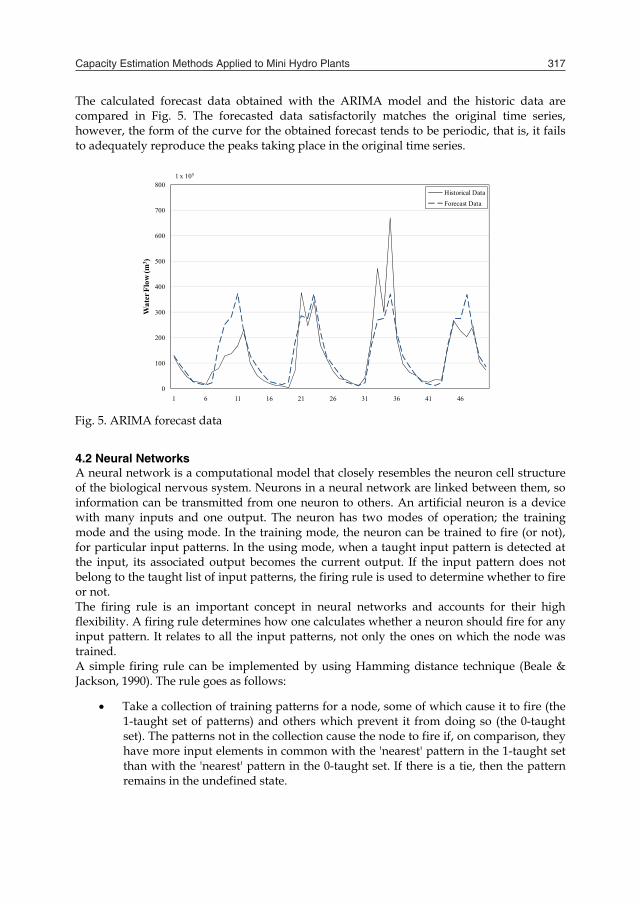
The calculated forecast data obtained with the ARIMA model and the historic data are compared in Fig. 5. The forecasted data satisfactorily matches the original time series, however, the form of the curve for the obtained forecast tends to be periodic, that is, it fails to adequately reproduce the peaks taking place in the original time series.
0
100
200
300
400
500
600
700
800
1 6 11 16 21 26 31 36 41 46
Wat
er F
low
(m3 )
Historical DataForecast Data
1 x 10⁵
Fig. 5. ARIMA forecast data
4.2 Neural Networks A neural network is a computational model that closely resembles the neuron cell structure of the biological nervous system. Neurons in a neural network are linked between them, so information can be transmitted from one neuron to others. An artificial neuron is a device with many inputs and one output. The neuron has two modes of operation; the training mode and the using mode. In the training mode, the neuron can be trained to fire (or not), for particular input patterns. In the using mode, when a taught input pattern is detected at the input, its associated output becomes the current output. If the input pattern does not belong to the taught list of input patterns, the firing rule is used to determine whether to fire or not. The firing rule is an important concept in neural networks and accounts for their high flexibility. A firing rule determines how one calculates whether a neuron should fire for any input pattern. It relates to all the input patterns, not only the ones on which the node was trained. A simple firing rule can be implemented by using Hamming distance technique (Beale & Jackson, 1990). The rule goes as follows:
Take a collection of training patterns for a node, some of which cause it to fire (the 1-taught set of patterns) and others which prevent it from doing so (the 0-taught set). The patterns not in the collection cause the node to fire if, on comparison, they have more input elements in common with the 'nearest' pattern in the 1-taught set than with the 'nearest' pattern in the 0-taught set. If there is a tie, then the pattern remains in the undefined state.
Capacity Estimation Methods Applied to Mini Hydro Plants 317
In order to describe the mathematics involved in an ARIMA model, it is important to define an ARMA(p, q) model for a data time series X(n), where n is an integer index to indicate a specific data within the time series, then an ARMA(p, q) model is given by (Ramachandran & Bhethanabotla, 2000)
(1-1
p
i i Li) X(n) = (1+
1
q
i θi Li) n (1)
where L is the lag operator, i are the auto-regressive parameters of the model, θi are the moving average parameters of the model, and n are error terms. The error terms n are usually known as white noise and they are assumed to be independent with zero co-variances, and identically distributed sampled data from a normal distribution with zero average. The ARIMA(p, d, q) model can be obtained integrating Equation (1). That is,
(1-1
p
i i Li ) (1-L)d X(n) = (1+
1
q
i θi Li) n (2)
where d is a positive integer that controls the level of differentiation. Note that if d = 0, this model is equivalent to an ARMA model. There are three basic steps to the development of an ARIMA model (Brockwell & Davis, 2002):
1) Identification/model selection: the values of p, d, and q must be determined. The principle of parsimony, also known as principle of simplicity, is adopted; most stationary time series can be modeled using very low values of p and q.
2) Estimation: the θ and the parameters must be estimated, usually by employing a least squares approximation to the maximum likelihood estimator.
3) Diagnostic checking: the estimated model must be checked for its adequacy and revised if necessary, implying that this entire process may have to be repeated until a satisfactory model is found.
The most crucial of these steps is identification, or model selection. This step requires the researcher to use his or her personal judgment to interpret some selected statistics, in conjunction with a graph from a set of autocorrelation coefficients, to determine which model the data suggest is the appropriate one to be employed. In this respect the ARIMA model is an art form, requiring considerable experience for a researcher to able to select the correct model. Using the R-Project software (R-Project, 2009), a model that allows the determination of each ARIMA parameters was implemented; 370 data points were used to obtain the model and the last 50 values of the time series were used to compare the forecast obtained by the model with the results from the historical time series. For an ARIMA (3, 1, 2) model, e.g. with three auto-regressive parameters (ARX), one integrator parameter (INTGX) and two moving average parameters (MAX), the coefficients shown in Table 1 were obtained.
AR1 AR2 AR3 MA1 MA2 INTG1 -0.1559 0.2239 0.0753 -0.5109 -0.4891 -0.4652
Table 1. ARIMA technique coefficients
The calculated forecast data obtained with the ARIMA model and the historic data are compared in Fig. 5. The forecasted data satisfactorily matches the original time series, however, the form of the curve for the obtained forecast tends to be periodic, that is, it fails to adequately reproduce the peaks taking place in the original time series.
0
100
200
300
400
500
600
700
800
1 6 11 16 21 26 31 36 41 46
Wat
er F
low
(m3 )
Historical DataForecast Data
1 x 10⁵
Fig. 5. ARIMA forecast data
4.2 Neural Networks A neural network is a computational model that closely resembles the neuron cell structure of the biological nervous system. Neurons in a neural network are linked between them, so information can be transmitted from one neuron to others. An artificial neuron is a device with many inputs and one output. The neuron has two modes of operation; the training mode and the using mode. In the training mode, the neuron can be trained to fire (or not), for particular input patterns. In the using mode, when a taught input pattern is detected at the input, its associated output becomes the current output. If the input pattern does not belong to the taught list of input patterns, the firing rule is used to determine whether to fire or not. The firing rule is an important concept in neural networks and accounts for their high flexibility. A firing rule determines how one calculates whether a neuron should fire for any input pattern. It relates to all the input patterns, not only the ones on which the node was trained. A simple firing rule can be implemented by using Hamming distance technique (Beale & Jackson, 1990). The rule goes as follows:
Take a collection of training patterns for a node, some of which cause it to fire (the 1-taught set of patterns) and others which prevent it from doing so (the 0-taught set). The patterns not in the collection cause the node to fire if, on comparison, they have more input elements in common with the 'nearest' pattern in the 1-taught set than with the 'nearest' pattern in the 0-taught set. If there is a tie, then the pattern remains in the undefined state.

Distributed Generation 318
Neurons in a neural network are linked between them, so information can be transmitted from one neuron to others. Given a data training set the neural network can learn the historic data through a training process and, with a learning algorithm the weights of the neurons are adjusted; through this procedure, the neural network acquires the capacity to predict answers of the same type of phenomenon. Activation functions are also needed in order to train the neural network; different activation functions are frequently used, including step, linear (or ramp), threshold, and sigmoid functions. In this research, the back-propagation learning algorithm (the most commonly used), was employed where the neural network forms a mapping between the inputs and the desired outputs from the training set by altering the weights of the connections within the network (Hilera & Martínez, 2000). Different types of neural networks have been developed depending on the characteristics and the type of application. Common applications of this computational model are: speech recognition, control systems, classification of patterns, identification of systems, time series forecast, etc. (Hilera & Martínez, 2000). A general structure of the connections of a neural network can be observed in Figure 6. During the phase of training, the connections weights Wij are iteratively calculated; these connections link the neurons of the inputs Ei with the neurons of the layer Oj. If an input is received, this is sent across the neurons of the layer, and the weights of the connections are then adjusted, generating an output S. This output is compared with the real input, generating an error, which is back-propagated from the output to the input; this iterative process is carried-out until the neural network is able to reproduce the input. The mathematical approach of the neural network working is as follows: A neuron in the output layer determines its activity by following a two step procedure.
First, it computes the total weighted input Ei, using the Equation:
Ei = j
yj Wij (3)
where yj is the activity level of the jth neuron in the previous layer. Next, the neuron calculates the activity yi, using a function of the total weighted
input. Typically the sigmoid function is used:
yi = 1/(1 + e-Ei) (4)
Once the activities of all output neurons have been determined, the network computes the error err, which is defined by the expression:
err = (1/2)j
( yj - dj)2 (5)
where dj is the desired output of the ith neuron.
Now, the back-propagation algorithm can be applied; it consists of four steps: 1) Compute how fast the error changes as the activity of an output neuron is changed.
This error derivative (EA) is the difference between the actual and the desired activity.
EAi = (∂err / yi) = yi - di (6)
2) Compute how fast the error changes as the total input received by an output neuron is changed. This quantity (EI) is the answer from step 1 multiplied by the rate at which the output of a neuron changes while its total input is changed.
EIi = (∂err / Ei) = (∂err / yi) × (∂yi / Ei) = EAi yi (1 - yi) (7)
3) Compute how fast the error changes as a weight of the connection into an output neuron is changed. This quantity (EW) is the answer from step 2 multiplied by the neuron activity level from which the connection emanates.
EWij = (∂err / Wij) = (∂err / Ei) × (∂Ei / Wij) = EIi yj (8)
4) Compute how fast the error changes as the activity of a neuron in the previous layer is changed. This crucial step allows back-propagation to be applied to multilayer networks. When the activity of a neuron in the previous layer changes, it affects the activities of all the output neurons to which it is connected. So, to compute the overall effect on the error, we add together all these separate effects on output neurons. But each effect is simple to calculate; it is the answer in step 2 multiplied by the weight on the connection to that output neuron.
EAj = (∂err / yj) = i
(∂err / Ei) × (∂Ei / yj) = i
EIi Wij (9)
By using steps 2 and 4, we can convert the EAs of one layer of neurons into EAs for the previous layer. This procedure can be repeated to get the EAs for as many previous layers as desired. Once we know the EA of a neuron, we can use steps 2 and 3 to compute the EWs on its incoming connections.
E1
E2
E3
O1
O2
O3
Ei Oj
S
Wji
W1,1
Wj
Fig. 6. General structure of the connections in a neural network For the case under consideration a neural network with 3 layers and 30 neurons for each layer was implemented in C language; 370 data from the Cardel Hydrometric station time series were used to train the neural network and 50 values were used for the validation of the obtained forecast. Figure 7 shows the results obtained with this computational technique and the corresponding comparison against the historical time series. From this figure it is possible to

Capacity Estimation Methods Applied to Mini Hydro Plants 319
Neurons in a neural network are linked between them, so information can be transmitted from one neuron to others. Given a data training set the neural network can learn the historic data through a training process and, with a learning algorithm the weights of the neurons are adjusted; through this procedure, the neural network acquires the capacity to predict answers of the same type of phenomenon. Activation functions are also needed in order to train the neural network; different activation functions are frequently used, including step, linear (or ramp), threshold, and sigmoid functions. In this research, the back-propagation learning algorithm (the most commonly used), was employed where the neural network forms a mapping between the inputs and the desired outputs from the training set by altering the weights of the connections within the network (Hilera & Martínez, 2000). Different types of neural networks have been developed depending on the characteristics and the type of application. Common applications of this computational model are: speech recognition, control systems, classification of patterns, identification of systems, time series forecast, etc. (Hilera & Martínez, 2000). A general structure of the connections of a neural network can be observed in Figure 6. During the phase of training, the connections weights Wij are iteratively calculated; these connections link the neurons of the inputs Ei with the neurons of the layer Oj. If an input is received, this is sent across the neurons of the layer, and the weights of the connections are then adjusted, generating an output S. This output is compared with the real input, generating an error, which is back-propagated from the output to the input; this iterative process is carried-out until the neural network is able to reproduce the input. The mathematical approach of the neural network working is as follows: A neuron in the output layer determines its activity by following a two step procedure.
First, it computes the total weighted input Ei, using the Equation:
Ei = j
yj Wij (3)
where yj is the activity level of the jth neuron in the previous layer. Next, the neuron calculates the activity yi, using a function of the total weighted
input. Typically the sigmoid function is used:
yi = 1/(1 + e-Ei) (4)
Once the activities of all output neurons have been determined, the network computes the error err, which is defined by the expression:
err = (1/2)j
( yj - dj)2 (5)
where dj is the desired output of the ith neuron.
Now, the back-propagation algorithm can be applied; it consists of four steps: 1) Compute how fast the error changes as the activity of an output neuron is changed.
This error derivative (EA) is the difference between the actual and the desired activity.
EAi = (∂err / yi) = yi - di (6)
2) Compute how fast the error changes as the total input received by an output neuron is changed. This quantity (EI) is the answer from step 1 multiplied by the rate at which the output of a neuron changes while its total input is changed.
EIi = (∂err / Ei) = (∂err / yi) × (∂yi / Ei) = EAi yi (1 - yi) (7)
3) Compute how fast the error changes as a weight of the connection into an output neuron is changed. This quantity (EW) is the answer from step 2 multiplied by the neuron activity level from which the connection emanates.
EWij = (∂err / Wij) = (∂err / Ei) × (∂Ei / Wij) = EIi yj (8)
4) Compute how fast the error changes as the activity of a neuron in the previous layer is changed. This crucial step allows back-propagation to be applied to multilayer networks. When the activity of a neuron in the previous layer changes, it affects the activities of all the output neurons to which it is connected. So, to compute the overall effect on the error, we add together all these separate effects on output neurons. But each effect is simple to calculate; it is the answer in step 2 multiplied by the weight on the connection to that output neuron.
EAj = (∂err / yj) = i
(∂err / Ei) × (∂Ei / yj) = i
EIi Wij (9)
By using steps 2 and 4, we can convert the EAs of one layer of neurons into EAs for the previous layer. This procedure can be repeated to get the EAs for as many previous layers as desired. Once we know the EA of a neuron, we can use steps 2 and 3 to compute the EWs on its incoming connections.
E1
E2
E3
O1
O2
O3
Ei Oj
S
Wji
W1,1
Wj
Fig. 6. General structure of the connections in a neural network For the case under consideration a neural network with 3 layers and 30 neurons for each layer was implemented in C language; 370 data from the Cardel Hydrometric station time series were used to train the neural network and 50 values were used for the validation of the obtained forecast. Figure 7 shows the results obtained with this computational technique and the corresponding comparison against the historical time series. From this figure it is possible to

Distributed Generation 320
observe that the neural network is able to forecast future data more accurately than the ARIMA method.
0
100
200
300
400
500
600
700
800
1 6 11 16 21 26 31 36 41 46 51
Wat
er F
low
(m3 )
Historical DataForecast Data
1 x 10⁵
Fig. 7. Neural network forecast data
4.3 Genetic Programming by ECSID Software Genetic Algorithms (GA) (Holland, 1992) and Gene Expression Programming (GEP) (Ferreira, 2006) are evolutionary tools inspired in the Darwinian principle of natural selection and survival of the fittest individuals. These methods use an initial random population and apply genetic operations to this population until the algorithm finds an individual that satisfies some termination criteria. In order to simulate the evolutionary process both GA and GEP follow the next steps:
1) Initialization: Creates an initial random population. 2) Evaluation: Evaluates all the individuals and test whether or not the best one
satisfies the termination criteria. 3) Selection: Use fitness proportional selection and apply the genetic operations to this
population.
GA uses a fixed chromosome structure, which can be an array of bits, numbers, characters, etc. To use GA the problem is codified as a fixed chromosome and then the problem is solved using an evolutionary process. The genetic operations more widely used are crossover, selection and mutation. GEP is similar to Genetic Programming (GP) (Koza, 1992); it is an evolutionary algorithm that evolves computer programs. The basic idea behind GEP is a clever representation for the chromosomes (a string instead of a tree), which leads to an easier implementation. ECSID stands for "Evolutionary Computation based System IDentification"; it is a program that makes mathematical models from an observation data set (Flores et al., 2005). ECSID obtains a formula that models the training data set, using a slide window prediction method (Jie et al., 2004). The slide window prediction method uses a window of size 16; the
window contains the actual data, and the model computes the synthetic time-series and the prediction errors for that time window. Equation (10) shows the general models generated by the software, where f(i) represents the time series at instant i, e(i) is the vector of prediction errors, h is the window size, and a, b are unknown coefficients to be find out by the software.
f(i+1) =
1t
i t h ai f(i) +
1t
i t h bi e(i) (10)
In order to make a forecast with this program, 337 data were used to obtain a model that represents the time series, and 83 data for the validation of the forecast obtained with the model. From the ECSID model, a forecast study was conducted, with the results compared against real data. The comparison is shown in Figure 8, where the predicted data tends to an irregular triangular waveform, which is repeated in constant oscillation periods of 12 data (one year). For the first 50 points, the model achieves an acceptable reproduction of the original time series under study.
5. Application to the Capacity Estimation of Mini Hydro Plants
With the results obtained from the previous section (forecast data) and the available historical data, it is possible to determine the design water flow Qi for the turbines of the mini hydro plant. It is also necessary to know the plant factor pf, which is the percentage of time that the plant is expected to be generating electric power at full capacity. The typical plant factor for this type of hydro plants varies from 0.70 to 0.85 (ITDG, 1996). The following procedure was used to determine the value of Qi:
A ten-year forecast is conducted using the time series; this period usually corresponds to the useful life of hydraulic turbines.
The obtained forecast data are added to the historical data, in this way, a more complete set of data of the river water flow is available.
A new flow duration curve can be built using the new data set. Different values of pf are now selected and the respective value of Qi from the
water flow duration curve is chosen.
A summary of the design water flow obtained for the new time series calculated from the different forecast techniques (at different typical plant factors), and the average monthly water flow Qm is shown in Table 2; the water flow is in 1105 m3. This Table illustrates that the neural network technique provided the most accurate results. The ARIMA and ECSID results suggest that the water flow in the river tends to be lower each year, that is, a smaller design water flow should be selected.

Capacity Estimation Methods Applied to Mini Hydro Plants 321
observe that the neural network is able to forecast future data more accurately than the ARIMA method.
0
100
200
300
400
500
600
700
800
1 6 11 16 21 26 31 36 41 46 51
Wat
er F
low
(m3 )
Historical DataForecast Data
1 x 10⁵
Fig. 7. Neural network forecast data
4.3 Genetic Programming by ECSID Software Genetic Algorithms (GA) (Holland, 1992) and Gene Expression Programming (GEP) (Ferreira, 2006) are evolutionary tools inspired in the Darwinian principle of natural selection and survival of the fittest individuals. These methods use an initial random population and apply genetic operations to this population until the algorithm finds an individual that satisfies some termination criteria. In order to simulate the evolutionary process both GA and GEP follow the next steps:
1) Initialization: Creates an initial random population. 2) Evaluation: Evaluates all the individuals and test whether or not the best one
satisfies the termination criteria. 3) Selection: Use fitness proportional selection and apply the genetic operations to this
population.
GA uses a fixed chromosome structure, which can be an array of bits, numbers, characters, etc. To use GA the problem is codified as a fixed chromosome and then the problem is solved using an evolutionary process. The genetic operations more widely used are crossover, selection and mutation. GEP is similar to Genetic Programming (GP) (Koza, 1992); it is an evolutionary algorithm that evolves computer programs. The basic idea behind GEP is a clever representation for the chromosomes (a string instead of a tree), which leads to an easier implementation. ECSID stands for "Evolutionary Computation based System IDentification"; it is a program that makes mathematical models from an observation data set (Flores et al., 2005). ECSID obtains a formula that models the training data set, using a slide window prediction method (Jie et al., 2004). The slide window prediction method uses a window of size 16; the
window contains the actual data, and the model computes the synthetic time-series and the prediction errors for that time window. Equation (10) shows the general models generated by the software, where f(i) represents the time series at instant i, e(i) is the vector of prediction errors, h is the window size, and a, b are unknown coefficients to be find out by the software.
f(i+1) =
1t
i t h ai f(i) +
1t
i t h bi e(i) (10)
In order to make a forecast with this program, 337 data were used to obtain a model that represents the time series, and 83 data for the validation of the forecast obtained with the model. From the ECSID model, a forecast study was conducted, with the results compared against real data. The comparison is shown in Figure 8, where the predicted data tends to an irregular triangular waveform, which is repeated in constant oscillation periods of 12 data (one year). For the first 50 points, the model achieves an acceptable reproduction of the original time series under study.
5. Application to the Capacity Estimation of Mini Hydro Plants
With the results obtained from the previous section (forecast data) and the available historical data, it is possible to determine the design water flow Qi for the turbines of the mini hydro plant. It is also necessary to know the plant factor pf, which is the percentage of time that the plant is expected to be generating electric power at full capacity. The typical plant factor for this type of hydro plants varies from 0.70 to 0.85 (ITDG, 1996). The following procedure was used to determine the value of Qi:
A ten-year forecast is conducted using the time series; this period usually corresponds to the useful life of hydraulic turbines.
The obtained forecast data are added to the historical data, in this way, a more complete set of data of the river water flow is available.
A new flow duration curve can be built using the new data set. Different values of pf are now selected and the respective value of Qi from the
water flow duration curve is chosen.
A summary of the design water flow obtained for the new time series calculated from the different forecast techniques (at different typical plant factors), and the average monthly water flow Qm is shown in Table 2; the water flow is in 1105 m3. This Table illustrates that the neural network technique provided the most accurate results. The ARIMA and ECSID results suggest that the water flow in the river tends to be lower each year, that is, a smaller design water flow should be selected.

Distributed Generation 322
0
100
200
300
400
500
600
700
800
1 11 21 31 41 51 61 71 81
Wat
er F
low
(m3 )
Historical DataForecast Data
1 x 10⁵
Fig. 8. ECSID forecast data The theoretical average power Pm obtained from the river can be estimated using Equation (11) (IDAE, 1996):
Pm = 9.81Qm H η γ (11)
where H is the height (m); η total efficiency of the system (p.u.); and γ is the specific weight of water (1 000 kg/m3). The Average Annual Generation of the system AAG is determined by (Penche, 1998),
AAG = (9.81Qi H η 8760 pf)/1106 (12)
Forecast Technique Qm
Qi Plant factor (pf)
0.70 0.75 0.80 0.85 Historic
data 147.894 42.283 32.874 28.398 24.414
ARIMA 115.733 31.326 27.356 23.161 19.488 Neural
Network 144.854 40.501 32.793 28.228 23.948
ECSID 135.733 38.442 30.907 24.918 22.872 Table 2. Design water flow For the case study, there are different places close to the Cardel hydrometric station with heights varying from 5 m to 15 m. These are locations where the construction of the civil work of the mini hydro plant can be built (CSVA, 2008). Equations (11) and (12) are applied to obtain the theoretical total generation of the system. The parameter η includes the effects of the losses in the whole system, e.g. for our case η is assumed to be 1.0 p.u.
Table 3 summarizes the power generation that can be obtained from this river based on the results achieved with the neural network method, considering a plant factor of 0.8, and a design water flow of 28.228 × 10⁵ m3 at different heights.
5 m 10 m 15 m Pm 355.254 kW 710.509 kW 1.065 MW
AAG 5.283 GWh 10.567 GWh 15.851 GWh Table 3. Average power and average annual generation of the system at different heights It can be observed from Table 3 that the ideal height to be considered for the design and the selection of the mini hydro plant components is between 10 to 15 meters (CSVA, 2008) where the maximum power from the river can be obtained. For the case of study a capacity of 1 MW was selected which corresponds to the maximum height (15 m).
6. Selections of Electromechanical Equipment
Fig. 9(a) illustrates the high head scheme of a mini hydro plant; this scheme uses weirs to divert water to the intake, from where it is conveyed to the turbines, via a pressure pipe or penstock. Fig 9(b) shows the electrical diagram of a mini hydro plant. The basic electro-mechanical equipment in these plants comprises the turbines, generators, transformers and the interconnecting power line. An appropriate design and selection of the mini hydro plant components based on the forecast techniques and the results reported in Section 4 and 5, are described next.
6.1 Hydraulic Turbine For the proposed case of study, the water flow design of 10.890 m3/s and a height of 15 m were selected. To know the specific characteristics of the selected turbine, it is necessary to have the charts, graphs and characteristics from the turbine manufacturer. In the Alstom’s web page (Alstom, 2009), a program that selects and presents the characteristics for the turbine-generator group used in a mini hydro plant can be accessed. Providing the water flow and height data, the program Mini Aqua Configurator (Alstom, 2009) shows a graph with the type of available turbines, as illustrated by Fig. 10, showing the exact position and the type of the selected turbine (square in the central part of the graph). The type of turbine to be selected for this case study can be Kaplan or Francis. The use of the Kaplan turbine is recommended since it is generally cheaper. The power generation estimated by the program for the turbine-generator group is 1.48 MW. Other relevant data are: 720 rpm, 88% of efficiency and 1320 mm for the diameter of the head turbine. 6.2 Generator The selection of the generator for the mini hydro plant is mainly based on the turbine characteristics. Thus, a synchronous generator was selected with the following specifications: 1.5 MVA, 380 V, 60 Hz, 720 rpm and 0.9 power factor.

Capacity Estimation Methods Applied to Mini Hydro Plants 323
0
100
200
300
400
500
600
700
800
1 11 21 31 41 51 61 71 81
Wat
er F
low
(m3 )
Historical DataForecast Data
1 x 10⁵
Fig. 8. ECSID forecast data The theoretical average power Pm obtained from the river can be estimated using Equation (11) (IDAE, 1996):
Pm = 9.81Qm H η γ (11)
where H is the height (m); η total efficiency of the system (p.u.); and γ is the specific weight of water (1 000 kg/m3). The Average Annual Generation of the system AAG is determined by (Penche, 1998),
AAG = (9.81Qi H η 8760 pf)/1106 (12)
Forecast Technique Qm
Qi Plant factor (pf)
0.70 0.75 0.80 0.85 Historic
data 147.894 42.283 32.874 28.398 24.414
ARIMA 115.733 31.326 27.356 23.161 19.488 Neural
Network 144.854 40.501 32.793 28.228 23.948
ECSID 135.733 38.442 30.907 24.918 22.872 Table 2. Design water flow For the case study, there are different places close to the Cardel hydrometric station with heights varying from 5 m to 15 m. These are locations where the construction of the civil work of the mini hydro plant can be built (CSVA, 2008). Equations (11) and (12) are applied to obtain the theoretical total generation of the system. The parameter η includes the effects of the losses in the whole system, e.g. for our case η is assumed to be 1.0 p.u.
Table 3 summarizes the power generation that can be obtained from this river based on the results achieved with the neural network method, considering a plant factor of 0.8, and a design water flow of 28.228 × 10⁵ m3 at different heights.
5 m 10 m 15 m Pm 355.254 kW 710.509 kW 1.065 MW
AAG 5.283 GWh 10.567 GWh 15.851 GWh Table 3. Average power and average annual generation of the system at different heights It can be observed from Table 3 that the ideal height to be considered for the design and the selection of the mini hydro plant components is between 10 to 15 meters (CSVA, 2008) where the maximum power from the river can be obtained. For the case of study a capacity of 1 MW was selected which corresponds to the maximum height (15 m).
6. Selections of Electromechanical Equipment
Fig. 9(a) illustrates the high head scheme of a mini hydro plant; this scheme uses weirs to divert water to the intake, from where it is conveyed to the turbines, via a pressure pipe or penstock. Fig 9(b) shows the electrical diagram of a mini hydro plant. The basic electro-mechanical equipment in these plants comprises the turbines, generators, transformers and the interconnecting power line. An appropriate design and selection of the mini hydro plant components based on the forecast techniques and the results reported in Section 4 and 5, are described next.
6.1 Hydraulic Turbine For the proposed case of study, the water flow design of 10.890 m3/s and a height of 15 m were selected. To know the specific characteristics of the selected turbine, it is necessary to have the charts, graphs and characteristics from the turbine manufacturer. In the Alstom’s web page (Alstom, 2009), a program that selects and presents the characteristics for the turbine-generator group used in a mini hydro plant can be accessed. Providing the water flow and height data, the program Mini Aqua Configurator (Alstom, 2009) shows a graph with the type of available turbines, as illustrated by Fig. 10, showing the exact position and the type of the selected turbine (square in the central part of the graph). The type of turbine to be selected for this case study can be Kaplan or Francis. The use of the Kaplan turbine is recommended since it is generally cheaper. The power generation estimated by the program for the turbine-generator group is 1.48 MW. Other relevant data are: 720 rpm, 88% of efficiency and 1320 mm for the diameter of the head turbine. 6.2 Generator The selection of the generator for the mini hydro plant is mainly based on the turbine characteristics. Thus, a synchronous generator was selected with the following specifications: 1.5 MVA, 380 V, 60 Hz, 720 rpm and 0.9 power factor.

Distributed Generation 324
Fig. 9. Mini hydro plant: a) High head scheme, b) Electrical diagram
6.3 Transformers For the proposed mini hydro plant, the use of three transformers is assumed; e.g. step-up, step-down transformers with a nominal capacity of 1.5 MVA and a transformer of 45 kVA for the self services in the plant. The proposed transformers have the following characteristics: 380 V / 13.2 kV to 60 Hz, Both the transformers will be connected in delta- wye grounded configuration.
Fig. 10. Diagram of the available turbines in Alstom for mini hydro plants (Alstom, 2009)
6.4 Interconnection Power Line According to CFE (Comisión Federal de Eléctricidad, México) construction norms (CFE, 1995), for this type of system the following primary distribution arrangement is recommended with the following characteristics: 3 phases, star connected, with solid connection to ground at the substation site. A simple cross-arm post type (TS) will be used for the distribution line.
7. Conclusion
In this chapter, a procedure for estimating the capacity of distributed generation based on mini hydro plants has been presented. This procedure has been successfully applied for a practical case where this type of distributed generation can be installed. The classic method used to estimate the capacity of a mini hydro plant was also introduced and then time series forecasting techniques were applied in order to enhance the historic data available. Based on the results of these forecast techniques and the available historical data, an estimation of the design water flow was performed, and a possible capacity for a mini hydro plant calculated. The time series forecast analysis has been conducted using an ARIMA model, a neural network and Genetic Programming by means of the software ECSID. For each case study, the obtained forecast results have been validated against actual measured data. The forecast technique based on neural networks has proven to give the best results for the case under consideration. Also, the selection of the most important electro-mechanic components of a proposed mini hydro plant based on the selected design water flow has been described.
8. References
Alstom. (2009). Mini Aqua Configurator. [Online]. Available: http://www.hydro.power.alstom.com/configurator/project_selection.html
Azadeh, A.; Ghaderia, S.F. & Sohrabkhania, S. (2007). Forecasting electrical consumption by integration of Neural Network, time series and ANOVA. Applied Mathematics and Computation, Vol. 182, No. 2, (March 2007), pp. 1753-1761, ISSN 0096-3003
Beale, R.; Jackson, T. (1990). Neural computing: an introduction, IOP Publishing Ltd, ISBN 0-85274-262-2, Bristol, UK
BHA. (2005). A guide to UK mini-hydro developments, The British Hydropower Association. London, UK
Brockwell, P. & Davis, R. (2002), Introduction to Time Series and Forecasting, Springer-Verlag, ISBN 0-387-95351-5, New York, USA
CFE. (1995). Normas de Distribución, construcción de líneas aéreas (Distribution norms, construction of electric lines), Comisión Federal de Electricidad, Mexico
CONAE. (2005). Situación Actual de la Minihidráulica Nacional y Potencial en una región de los Estados de Veracruz y Puebla (Current Situation of the National Mini-hydro and the Potential Available for the States of Veracruz and Puebla, Mexico), Comisión Nacional de Ahorro de Energía, Mexico
CSVA. (2008). Consejo del Sistema Veracruzano del Agua. [Online]. Available: http://www.csva.gob.mx
Ferreira, C. (2006). Gene Expression Programming: Mathematical Modeling by an Artificial Intelligence, Springer-Verlag, ISBN 3540327967, Berlin, Germany
Flores, J.J.; Graff, M. & Cardenas, E. (2005). Wind Prediction Using Genetic Algorithms and Gene Expression Programming. Proceedings of AMSE 2005, pp. 17-26, Morelia, Mexico, April 2005
Hamilton, J.D. (1994). Time series analysis, Princeton University Press, ISBN 0-691-04289-6, New Jersey, USA

Capacity Estimation Methods Applied to Mini Hydro Plants 325
Fig. 9. Mini hydro plant: a) High head scheme, b) Electrical diagram
6.3 Transformers For the proposed mini hydro plant, the use of three transformers is assumed; e.g. step-up, step-down transformers with a nominal capacity of 1.5 MVA and a transformer of 45 kVA for the self services in the plant. The proposed transformers have the following characteristics: 380 V / 13.2 kV to 60 Hz, Both the transformers will be connected in delta- wye grounded configuration.
Fig. 10. Diagram of the available turbines in Alstom for mini hydro plants (Alstom, 2009)
6.4 Interconnection Power Line According to CFE (Comisión Federal de Eléctricidad, México) construction norms (CFE, 1995), for this type of system the following primary distribution arrangement is recommended with the following characteristics: 3 phases, star connected, with solid connection to ground at the substation site. A simple cross-arm post type (TS) will be used for the distribution line.
7. Conclusion
In this chapter, a procedure for estimating the capacity of distributed generation based on mini hydro plants has been presented. This procedure has been successfully applied for a practical case where this type of distributed generation can be installed. The classic method used to estimate the capacity of a mini hydro plant was also introduced and then time series forecasting techniques were applied in order to enhance the historic data available. Based on the results of these forecast techniques and the available historical data, an estimation of the design water flow was performed, and a possible capacity for a mini hydro plant calculated. The time series forecast analysis has been conducted using an ARIMA model, a neural network and Genetic Programming by means of the software ECSID. For each case study, the obtained forecast results have been validated against actual measured data. The forecast technique based on neural networks has proven to give the best results for the case under consideration. Also, the selection of the most important electro-mechanic components of a proposed mini hydro plant based on the selected design water flow has been described.
8. References
Alstom. (2009). Mini Aqua Configurator. [Online]. Available: http://www.hydro.power.alstom.com/configurator/project_selection.html
Azadeh, A.; Ghaderia, S.F. & Sohrabkhania, S. (2007). Forecasting electrical consumption by integration of Neural Network, time series and ANOVA. Applied Mathematics and Computation, Vol. 182, No. 2, (March 2007), pp. 1753-1761, ISSN 0096-3003
Beale, R.; Jackson, T. (1990). Neural computing: an introduction, IOP Publishing Ltd, ISBN 0-85274-262-2, Bristol, UK
BHA. (2005). A guide to UK mini-hydro developments, The British Hydropower Association. London, UK
Brockwell, P. & Davis, R. (2002), Introduction to Time Series and Forecasting, Springer-Verlag, ISBN 0-387-95351-5, New York, USA
CFE. (1995). Normas de Distribución, construcción de líneas aéreas (Distribution norms, construction of electric lines), Comisión Federal de Electricidad, Mexico
CONAE. (2005). Situación Actual de la Minihidráulica Nacional y Potencial en una región de los Estados de Veracruz y Puebla (Current Situation of the National Mini-hydro and the Potential Available for the States of Veracruz and Puebla, Mexico), Comisión Nacional de Ahorro de Energía, Mexico
CSVA. (2008). Consejo del Sistema Veracruzano del Agua. [Online]. Available: http://www.csva.gob.mx
Ferreira, C. (2006). Gene Expression Programming: Mathematical Modeling by an Artificial Intelligence, Springer-Verlag, ISBN 3540327967, Berlin, Germany
Flores, J.J.; Graff, M. & Cardenas, E. (2005). Wind Prediction Using Genetic Algorithms and Gene Expression Programming. Proceedings of AMSE 2005, pp. 17-26, Morelia, Mexico, April 2005
Hamilton, J.D. (1994). Time series analysis, Princeton University Press, ISBN 0-691-04289-6, New Jersey, USA

Distributed Generation 326
Hilera, J.R. & Martínez, V.J. (2000). Redes neuronales artificiales. Fundamentos, modelos y aplicaciones (Artificial Neural Networks, fundaments, models and applications), Alfaomega Ra-Ma, ISBN 8478971556, Madrid, Spain
Holland, J. H. (1992). Adaptation in Natural and Articial Systems, University of Michigan Press, ISBN 0-262-58111-6, Massachusetts, USA
IDAE. (1996). Manual of renewable energies: Mini hydroelectric power stations, Ministry of Economy, Madrid, Spain
ITDG. (1996). Manual de Mini y Microcentrales Hidráulicas; una guía para el desarrollo de proyectos (Mini and Micro-Hydraulic Plants; a project development guide), Intermediate Technology Development Group, Peru
Jie, Z.; Changjie, T. Chuan, L. Anlong C. & Chang'an, Y. (2004). Time series prediction based on gene expression programming. Proceedings of WAIM 2004, pp. 55-64, ISBN 978-3-540-22418-1, Dalian, China, September 2004
Khennas; Smail & Barnett, A. (2000). Best practices for sustainable development of micro hydro power in developing countries, World Bank / ESMAP, Madrid, Spain
Koza, J.R. (1992), Genetic Programming: On the Programming of Computers by Means of Natural Selection (Complex Adaptive Systems), The MIT Press, ISBN 0-262-11170-5, Massachusetts, USA
Montañés, E.; Quevedo, J.R. Prieto, M.M. & Menéndez, C.O. (2002). Forecasting Time Series Combining Machine Learning and Box-Jenkins Time Series. Proceedings of IBERAMIA 2002, pp. 491-499, ISBN 978-3-540-00131-7, Seville, Spain, January 2002
Penche, C. (1998). Layman’s book: on how to develop a small hydro site, European Small Hydropower Association (ESHA), Brussels, Belgium
Peña, R.; Medina, A., Anaya-Lara, O. & McDonald, J.R. (2009). Capacity estimation of a minihydro plant based on time series forecasting, Elsevier Renewable Energy, Vol. 34, No. 5, (May 2009), pp. 1204-1209, ISSN 0960-1481
Puttgen, H.B.; MacGregor, P.R. & Lambert, F.C. (2003). Distributed generation: Semantic hype or the dawn of a new era? IEEE Power and Energy Magazine, Vol. 1, No. 1, (January-February 2003), pp. 22-29, ISSN 1540-7977
Ramachandran, R. & Bhethanabotla, V.N. (2000). Generalized autoregressive moving average modeling of the Bellcore data. Proceedings of LCN 2000, pp. 654-661, ISBN 0-7695-0912-6, Tampa, USA, November 2000
R-Project. (2009). The R Project for Statistical Computing. [Online]. Available: http://www.r-project.org/
Sorensen, J.V.T. & Madsen, H. (2003). Water level prediction skill of an operational marine forecast using a hybrid Kalman filter and time series modeling approach. Proceedings of OCEANS 2003, pp. 790-796, ISBN 0-933957-30-0, San Diego, USA, September 2003
Xie, J.; Tang, X. & Li, T. (2006). Low Power Design based on Neural Network Forecasting for Interconnection Networks. Proceedings of WCICA 2006, pp. 2979-2983, ISBN 1-4244-0332-4, Dalian, China, June 2006
Zhou, M.; Yan, Z. Ni, Y. & Li, G. (2004). An ARIMA approach to forecasting electricity price with accuracy improvement by predicted errors. Proceedings of IEEE Power Engineering Society General Meeting 2004, pp. 233-238, ISBN 0-7803-8465-2, Denver, USA, June 2004