Scalable Visual Hierarchy Exploration - Worcester …davis.wpi.edu/~xmdv/docs/stroe_msthesis.pdf · · 2003-04-211.1 Caching and Prefetching for Large-Scale Visualization ... without

Scalable Visual Hierarchy Exploration

by

Ionel Daniel Stroe

A Thesis

Submitted to the Faculty

of the

WORCESTER POLYTECHNIC INSTITUTE

In partial fulfillment of the requirements for the

Degree of Master of Science

in

Computer Science

by

May 2000

APPROVED:

Professor Elke A. Rundensteiner, Thesis Advisor

Professor Matthew O. Ward, Thesis Advisor

Professor Carolina Ruiz, Thesis Reader

Professor Micha Hofri, Head of Department

Cu dragoste, parintilor mei.

Abstract

More and more modern computer applications, from business decision support to

scientific data analysis, utilize visualization techniques to support exploratory activities.

Most visualization tools do not scale well with regard to the size of the dataset upon

which they operate. Specifically, the level of cluttering on the screen is typically unac-

ceptable and the performance is poor. To solve the problem of cluttering at the interface

level, visualization tools have recently been extended to support hierarchical views of the

data, with support for focusing and drilling-down using interactive brushes. To solve the

scalability problem, this thesis investigates how best to couple a visualization tool with a

database management system without losing the real-time responsiveness required in any

interactive application.

This integration must be done carefully. Visual user interactions often cannot be ef-

ficiently realized using standard database operations. In our context, the recursive pro-

cessing required for the visual data retrieval was prohibitively expensive; responding for

instance to a single user request took up to 30 minutes on a 200,000 tuple dataset. We suc-

cessfully address this problem by developing a tree labeling method, called MinMax tree,

that moves the recursive processing into an off-line precomputation step. Thus, at run

time, the recursive operations translate into linear cost range queries. To further reduce

the response time, we employ a main memory access strategy to support incremental

loading of data into main memory. We also proposed a novel prefetching technique to

bring data into memory when the system is idle. Prefetching is speculative, non-pure, and

adaptive. These techniques have been incorporated into XmdvTool, a multidimensional

visual exploration tool, in order to achieve scalability. The tool now efficiently scales up

to datasets of order 105� 107 records. Lastly, we report experimental results to assess the

performance of the proposed techniques.

Acknowledgements

Many thanks to my professors and to my friends for their support.

This work is supported under NSF grant IIS-9732897 and NSF CISE Instrumentation

grant IRIS 97-29878.

i

Contents

1 Introduction 1

1.1 Caching and Prefetching for Large-Scale Visualization . . . . . . . . . . 1

1.2 Our Approach . . . . . . . . . . . . . . . . . . . . . . . . . . . . . . . . 3

1.3 Contributions . . . . . . . . . . . . . . . . . . . . . . . . . . . . . . . . 4

1.4 Thesis Organization . . . . . . . . . . . . . . . . . . . . . . . . . . . . . 5

2 Related Work 6

2.1 Visual Hierarchy Exploration . . . . . . . . . . . . . . . . . . . . . . . . 6

2.2 Visualization-Database Integrated Systems . . . . . . . . . . . . . . . . . 7

2.3 Relational Processing of Hierarchies . . . . . . . . . . . . . . . . . . . . 7

2.3.1 Join Processing . . . . . . . . . . . . . . . . . . . . . . . . . . . 7

2.3.2 Hierarchy Encoding . . . . . . . . . . . . . . . . . . . . . . . . 9

2.4 Main Memory Processing . . . . . . . . . . . . . . . . . . . . . . . . . . 10

2.4.1 High Level Caching . . . . . . . . . . . . . . . . . . . . . . . . 10

2.4.2 Prefetching . . . . . . . . . . . . . . . . . . . . . . . . . . . . . 10

3 Multivariate Data Visualization 12

3.1 Brush Basics . . . . . . . . . . . . . . . . . . . . . . . . . . . . . . . . 13

3.2 Hierarchical Clustering . . . . . . . . . . . . . . . . . . . . . . . . . . . 15

3.3 Structure-Based Brushes . . . . . . . . . . . . . . . . . . . . . . . . . . 17

ii

3.3.1 Creation and Manipulation . . . . . . . . . . . . . . . . . . . . . 17

3.3.2 Geometric Representation . . . . . . . . . . . . . . . . . . . . . 19

3.3.3 Multidimensional Extension . . . . . . . . . . . . . . . . . . . . 19

3.4 Model Abstraction . . . . . . . . . . . . . . . . . . . . . . . . . . . . . 20

4 Query Specification and Processing 24

4.1 MinMax Hierarchy Encoding . . . . . . . . . . . . . . . . . . . . . . . . 24

4.2 Query Processing Using MinMax . . . . . . . . . . . . . . . . . . . . . 26

4.2.1 Static Tree Hierarchies . . . . . . . . . . . . . . . . . . . . . . . 26

4.2.2 Dynamic Tree Hierarchies . . . . . . . . . . . . . . . . . . . . . 28

4.2.3 Arbitrary Hierarchies . . . . . . . . . . . . . . . . . . . . . . . . 30

5 Memory Management 33

5.1 Caching . . . . . . . . . . . . . . . . . . . . . . . . . . . . . . . . . . . 33

5.1.1 Semantic Caching . . . . . . . . . . . . . . . . . . . . . . . . . 34

5.1.2 Probabilistic Model . . . . . . . . . . . . . . . . . . . . . . . . . 36

5.1.3 Cache Replacement . . . . . . . . . . . . . . . . . . . . . . . . . 39

5.1.4 Database Intensive Case . . . . . . . . . . . . . . . . . . . . . . 44

5.2 Prefetching . . . . . . . . . . . . . . . . . . . . . . . . . . . . . . . . . 47

5.2.1 General Characteristics . . . . . . . . . . . . . . . . . . . . . . . 47

5.2.2 Strategies . . . . . . . . . . . . . . . . . . . . . . . . . . . . . . 48

6 Implementation 50

6.1 System Architecture . . . . . . . . . . . . . . . . . . . . . . . . . . . . . 50

6.2 Threads and Synchronization . . . . . . . . . . . . . . . . . . . . . . . . 51

6.3 Interacting with the Database . . . . . . . . . . . . . . . . . . . . . . . . 52

iii

7 Experimental Results 54

7.1 Experimental Inputs . . . . . . . . . . . . . . . . . . . . . . . . . . . . . 54

7.2 Settings . . . . . . . . . . . . . . . . . . . . . . . . . . . . . . . . . . . 56

7.3 Experiments . . . . . . . . . . . . . . . . . . . . . . . . . . . . . . . . . 57

8 Conclusions and Future Work 66

8.1 Conclusions . . . . . . . . . . . . . . . . . . . . . . . . . . . . . . . . . 66

8.2 Future Work . . . . . . . . . . . . . . . . . . . . . . . . . . . . . . . . . 68

A Navigation Operations 69

A.1 Notation Conventions . . . . . . . . . . . . . . . . . . . . . . . . . . . . 69

A.2 Hierarchical Clustering . . . . . . . . . . . . . . . . . . . . . . . . . . . 69

A.3 Structure Based Brushes . . . . . . . . . . . . . . . . . . . . . . . . . . 70

A.3.1 The ALL Structure Based Brush . . . . . . . . . . . . . . . . . . 71

A.3.2 The ANY Structure Based Brush . . . . . . . . . . . . . . . . . . 71

A.3.3 The Relational Semantics of Structure-Based Brushes . . . . . . 72

B MinMax Hierarchy Encoding 73

B.1 Proof of Theorem 1 . . . . . . . . . . . . . . . . . . . . . . . . . . . . . 74



C Complexity of Memory Operations 77

C.1 Full Size Probability Table . . . . . . . . . . . . . . . . . . . . . . . . . 78

C.2 Reduced Probability Table . . . . . . . . . . . . . . . . . . . . . . . . . 79

iv

List of Figures

1.1 Architecture of main memory-based implementation. . . . . . . . . . . . 3

1.2 Architecture of database-based implementation. Additional computation

steps are I/O intensive. . . . . . . . . . . . . . . . . . . . . . . . . . . . 3

3.1 Structure-based brush as combination of a focus region (a) and a density

factor (b). . . . . . . . . . . . . . . . . . . . . . . . . . . . . . . . . . . 15

3.2 Structure-based brush as combination of a horizontal (a) and a vertical (b)

selection. . . . . . . . . . . . . . . . . . . . . . . . . . . . . . . . . . . 15

3.3 Partition map for a tree hierarchy. . . . . . . . . . . . . . . . . . . . . . 16

3.4 Hierarchical tree obtained by clustering. . . . . . . . . . . . . . . . . . . 16

3.5 Structure-based brushing interface in XmdvTool. (a) Hierarchical tree

frame; (b) Contour corresponding to current level-of-detail; (c) Leaf con-

tour approximates shape of hierarchical tree; (d) Structure-based brush;

(e) Interactive brush handles; (f) Color map legend for level-of-detail con-

tour. . . . . . . . . . . . . . . . . . . . . . . . . . . . . . . . . . . . . . 18

3.6 ALL initial selection with brush values 3 and 7. . . . . . . . . . . . . . . 18

3.7 ANY initial selection with brush values 3 and 7. . . . . . . . . . . . . . . 18

3.8 2-D hierarchy map. Uniform levels of detail. . . . . . . . . . . . . . . . . 20

3.9 2-D hierarchy map. Arbitrary level of detail function. . . . . . . . . . . . 20

3.10 Selection space abstraction. . . . . . . . . . . . . . . . . . . . . . . . . . 21

v

3.11 Active window in the selection space. . . . . . . . . . . . . . . . . . . . 21

3.12 A tree example. . . . . . . . . . . . . . . . . . . . . . . . . . . . . . . . 21

3.13 Navigation on a tree support set. . . . . . . . . . . . . . . . . . . . . . . 21

3.14 Navigation grid. . . . . . . . . . . . . . . . . . . . . . . . . . . . . . . . 22

3.15 Active window. . . . . . . . . . . . . . . . . . . . . . . . . . . . . . . . 22

3.16 Base set. . . . . . . . . . . . . . . . . . . . . . . . . . . . . . . . . . . . 22

3.17 Objects on the same level are totally ordered. . . . . . . . . . . . . . . . 22

4.1 A continuous MinMax tree. . . . . . . . . . . . . . . . . . . . . . . . . . 25

4.2 A discrete MinMax tree. . . . . . . . . . . . . . . . . . . . . . . . . . . 25

4.3 An ALL structure-based brush. . . . . . . . . . . . . . . . . . . . . . . . 27

4.4 An ANY structure-based brush. . . . . . . . . . . . . . . . . . . . . . . 28

4.5 The allocation strategy. . . . . . . . . . . . . . . . . . . . . . . . . . . . 30

4.6 An arbitrary hierarchy. . . . . . . . . . . . . . . . . . . . . . . . . . . . 31

4.7 Bottom-up labeling of an arbitrary hierarchy. . . . . . . . . . . . . . . . 31

5.1 LA=0: two regions of equal probability, 0 and 1. . . . . . . . . . . . . . . 37

5.2 LA=1: five regions of equal probability, 0, 1, ..., 4. . . . . . . . . . . . . . 37

5.3 LA=2: ten regions of equal probability, 0, 1, ..., 9. . . . . . . . . . . . . . 39

5.4 Buffer content for a three level, twelve object example in case of a re-

duced probability table. . . . . . . . . . . . . . . . . . . . . . . . . . . . 42

5.5 Finishing reading. Current objects are painted solid; the overwritten ob-

jects striped. Dashed lines are undefined pointers. . . . . . . . . . . . . . 45

5.6 Starting re-reading. The traversal direction changes for both consumer

and producer. Buffer in an inconsistent state. . . . . . . . . . . . . . . . . 45

vi

6.1 System architecture. The ovals depict the flat-file data. Dashed-line rect-

angles show the separation between the on-line and the off-line computa-

tion. Solid-line rectangles represent the agents. Squares represent meta-

knowledge. Solid arrows show the control flow. . . . . . . . . . . . . . . 52

6.2 System synchronization. The dashed-line rectangle represents the main

thread. The rectangles on the left hand side of the main thread form the

prefetcher thread. The GUI acts as a separate process, due to the priority

queues of TK. . . . . . . . . . . . . . . . . . . . . . . . . . . . . . . . . 53

7.1 Hot regions: selections in the navigation space that provide useful insight

into the data. . . . . . . . . . . . . . . . . . . . . . . . . . . . . . . . . . 55

7.2 MinMax vs. Recursive. Structure-based brushes for dataset D1. . . . . . 58



7.5 Varying the level value. Functions compared against 2x. Logarithmic y

scale. . . . . . . . . . . . . . . . . . . . . . . . . . . . . . . . . . . . . 59

7.6 Varying the extent value. Functions compared against x�

1. . . . . . . . 59

7.7 Varying the dataset size. Levels 12 and 14 not defined for D1. . . . . . . 59

7.8 Varying the delays for strategy S2 and S3. Measured quality. . . . . . . . 60

7.9 Varying the delays for strategy S2 and S3. Measured hit ratio. . . . . . . 60

7.10 Varying the delays for strategy S2 and S3. Measured latency. . . . . . . . 61

7.11 Varying the delays for various datasets. Measured quality. . . . . . . . . . 61

7.12 Varying the number of hot regions. Measured both query and object hit

ratio. . . . . . . . . . . . . . . . . . . . . . . . . . . . . . . . . . . . . . 61

7.13 Varying the “keep direction” factor. Measured query and object hit ratio. . 61

7.14 Varying the “keep direction” factor for various datasets. Measured the hit

ratio. . . . . . . . . . . . . . . . . . . . . . . . . . . . . . . . . . . . . . 62

vii

7.15 Varying prefetching strategy. Measured object and query hit ratio. . . . . 62

7.16 Varied prefetching strategy for D1k10k. Measured the latency. . . . . . . 63

7.17 Varied prefetching strategy for D1k1M. Measured the latency. . . . . . . 63

7.18 Providing hints to the query optimizer. Varying the prefetching strategy.

Measured the hit ratio. . . . . . . . . . . . . . . . . . . . . . . . . . . . 63

7.19 Providing hints to the query optimizer. Varying the data size. Measured

the latency. . . . . . . . . . . . . . . . . . . . . . . . . . . . . . . . . . 63

7.20 Varying the dataset. Measured the hit ratio. . . . . . . . . . . . . . . . . 64

7.21 Varying the dataset. Measured the latency. . . . . . . . . . . . . . . . . . 64

viii

List of Tables

ix

Chapter 1

Introduction

1.1 Caching and Prefetching for Large-Scale Visualiza-

tion

Visualization provides effective techniques for the analysis of data. While statistics offers

us various tools for testing model hypotheses and finding model parameters, the task of

guessing the right type of model to use is still a process that cannot be automated. Thus,

whether the domain is stock data, scientific data, or the distribution of sales, visualization

plays an important role in the analysis. Humans can sometimes detect patterns and trends

in the underlying data by just looking at it, without being aware in advance about what

data model they’ll face.

Human perception is of course greatly influenced by the way data is presented. Thus,

various techniques for displaying data have been proposed over the years, each of which

focuses on emphasizing some of the data characteristics [1, 26, 8, 14, 30]. However,

most of these techniques do not scale well with respect to the size of the data. As a

generalization, [17] postulates that any method that displays a single entity per data point

invariably results in overlapped elements and a convoluted display that is not suited for

1

the visualization of large datasets.

A new approach has been proposed recently for displaying large datasets [16]. The

idea there is to present data at different levels of detail based on applying an aggregation

function to a hierarchical structure, structure that might result for instance from a cluster-

ing process. The problem of cluttering at the interface level is solved by displaying only

a limited set of aggregates at a time. However, such hierarchical summarizations increase

the size of data to be managed by at least one order of magnitude.

Storing and retrieving the data sets efficiently has often been ignored in the context

of visualization applications. While storing the data in main memory and flat files is

appropriate for small and moderate sized datasets, it becomes unacceptable when scaling

to large datasets. One possible solution to enable scaling is to integrate visualization

applications with database management systems. The last couple of decades of research

in the area of databases can greatly contribute to increasing the performance of a data

intensive application such as exploratory visualization.

Coupling a database with the visualization tool cannot be performed blindly though.

Techniques used for main memory processing are typically not efficient any more if im-

plemented directly in a database environment. A trivial and well known example is sort-

ing. Internal sorting strategies differ significantly from external sorting ones. Another

example is presented in this work: the recursive processing involved when navigating

through hierarchies in main memory is no longer appropriate when storing those hier-

archies on the disk. Instead, we propose a technique called MinMax trees [40, 41] that

transforms the recursive processing into fast range queries.

In general, there are two questions to be answered when doing such an integration

between visualization and database tools. The first is how to most effectively translate

the visual exploration operations such as zooming and brushing into a database under-

standable language such as SQL. The second is how to store and manage the results of

2

the database requests in main memory and make subsequent memory access operations

as efficient as possible. This work gives solutions for both questions.

1.2 Our Approach

Our approach to reducing the system latency (i.e., the on-line computation time) is to

push expensive computations off-line whenever possible. Visual tools require data to be

in the same address space to access it. In a simple main memory system, the data resides

entirely in the main memory (Fig. 1.1). When the visualization tool issues a request, the

entire computation is performed “on-demand” (i.e., on-line). The result is a set of objects

(datapoints) that is then passed back to the front-end. When the data is moved from the

main memory to persistent storage, two additional steps have to be present (Fig. 1.2).

First, the request needs to be translated into a format which is supported by the query

processor and then passed to the database for processing (also on-line). Second, the result

set needs to be loaded into the main memory and sent to the front-end for display. The

“on-demand” computation as well as data loading are I/O intensive and thus no longer

fast (compared to the main memory case). Our goal of minimizing the system latency can

be achieved by optimizing these two steps.

Figure 1.1: Architecture ofmain memory-based im-plementation.

Figure 1.2: Architecture of database-based imple-mentation. Additional computation steps are I/O in-tensive.

Our approach to making the first step efficient is to move part of the on-line compu-

3

tation into a pre-processing phase. In our case, the front-end operations are reducible to

a particular class of recursive unions of joins and divisions that operate on hierarchies.

By using adequate pre-computation (i.e., organizing the hierarchical structure into what

we call a MinMax tree), the recursive processing of the operations in this class can be

reduced to range queries. Extensions of our method for non-tree as well as for dynamic

hierarchies have also been designed (Chapter 4). Compared with alternate approaches to

similar problems from the literature [7, 44], our hierarchy labeling method is shown to

be superior in terms of both efficiency and functionality. The previous proposed methods

either do not support dynamic and arbitrary hierarchies, or were not able to efficiently

scale to large datasets.

To make the second step efficient, we employ a main memory strategy that supports

incremental loading of data into the main memory. We show that incremental loading is

highly desirable, given the set of operations to support (Chapter 5). To further reduce the

response time, we have designed a speculative prefetcher that brings data into memory

when the system is idle. The prefetcher is based on the property of exploratory systems

that queries remains “local”, i.e., given the set of currently selected objects we have a

small number of choices of which objects can be selected next. The property provides

therefore “implicit hints” to the system. Additional hints might be provided by the the

data and the user’s exploration as well.

1.3 Contributions

Our main contribution consists of developing a set of techniques that can be applied to

interactive visualization tools in order to enable them to explore large datasets. The char-

acteristics of the system to which these techniques can be applied to are presented in

Chapter 2.

4

We first designed and implemented an encoding technique that efficiently supports

on-line retrieval of data. We further designed a high level cache policy that reduces the

latency in the system by incrementally loading the data into the memory buffer. When

the system is idle, a prefetcher will bring into cache the data that is likely to be used

next. For this purpose, we used a novel technique that combines a low granularity of

data (object level) and a “semantic” description of the content of the buffer. We also

performed experiments to assess the efficiency of our approach. First, we tested our

encoding technique as a stand-alone method and found that it performed and scaled well.

Second, we tested the system to work with various input and under different settings. The

system scales well to support millions of data points with between 8 and 20 dimensions.

We confirmed the important role of precomputation in such applications and showed that

the benefit of using prefetching exceeds significantly the result from using the cache only.

1.4 Thesis Organization

Chapter 2 presents the related research from both the visualization and the database per-

spective. Chapter 3 introduces basic concepts in visualization and describes our approach

to achieve scalability from a front-end perspective. It also formalizes the requirements

under which our proposed approach works. The hierarchy encoding as well as the pro-

cessing of MinMax queries is further presented in Chapter 4. Chapter 5 introduces the

memory management, specifically the caching and prefetching strategies. The imple-

mentation of the system is discussed in Chapter 6. Experimental results are reported in

Chapter 7. Finally, we present conclusions as well as directions for further research in

Chapter 8.

5

Chapter 2

Related Work

2.1 Visual Hierarchy Exploration

There has been considerable research in the visualization area toward finding effective

methods to display and explore hierarchical information, such as Tree-Maps [37], Cone-

Trees [32] and Reconfigurable Disc Trees [22]. Most of these methods provide only

modest modes of interaction for navigating the hierarchy. Navigation plays an important

role in aiding users to find their way through the complex structure: to see where they are,

what information is available and how to identify information of interest.

On the other hand, techniques for visual exploration of hierarchies [27] have indepen-

dently been proposed. Hierarchy visualizations are evident for instance in many commer-

cial applications, such as Microsoft Windows Explorer, Norton Commander, and so on.

The major disadvantage of such interfaces however is that there is a limited display space

for the hierarchy. Hence, they are not suitable for displaying large data sets. The visu-

alization technique we use in this work [16, 17] has both the capability of interactively

navigating the hierarchical structures and the capability of displaying large datasets.

6

2.2 Visualization-Database Integrated Systems

Integrated visualization-database systems such as Tioga [39], IDEA [34], and DEVise

[28] represent the work closest related to ours in terms of problem area. The approaches

are however different. Tioga [39] implements a multiple browser architecture for what

they call a recipe, a visual query. The system is able to buffer the computed data; however,

the problem of translating front-end operations into database queries is not present since

database queries are directly (explicitly) specified by the graphical interface. IDEA [34]

is an integrated set of tools to support interactive data analysis and exploration. Some

constraints on the data model are imposed by the application domain, but on-line query

translation and memory management are not addressed. In DEVise [28], a set of query

and visualization primitives to support data analysis is provided. The number of primi-

tives supported is itself relatively large. However, caching data is done at the database

level using default mechanisms only; special memory management techniques are not

considered.

Other work in the same area includes dynamic query interfaces [43, 21], dynamic

query histograms [13] and direct manipulation query interfaces [20, 24, 19]. They all have

a visual interface and a database back-end. However, the operations translate differently:

to dynamic range queries in [13], to temporal queries in [20], and to 2-D spatial queries

in [24]. These works do not deal with hierarchy exploration support.

2.3 Relational Processing of Hierarchies

2.3.1 Join Processing

In relational systems, hierarchies (as composite objects) have to be broken down into

multiple fragments that are then stored as tuples in separate relations [46]. Traversing the

7

hierarchical structure in order to gather all fragments together or to query specific prop-

erties requires a large number of joins. Since relational joins are expensive operations, an

immediate improvement in handling hierarchical structures is achieved by improving join

efficiency.

Valduriez et al. [45] introduce a new access path for processing joins, called a join

index. The join index is simply a binary relation that contains pairs of surrogates (unique

system identifiers) of the tuples that are to be joined. An algorithm that uses join indices

is also presented in [45]. The join index efficiently supports the computation of joins and

particularly the join composition of complex objects in the case of a decomposed storage

representation [46].

Another method that speeds up join processing uses hidden pointer fields to link the

tuples to be joined. The hidden pointers are special attributes that contain record identi-

fiers. Three pointer-based join algorithms, simple variants of the nested-loops, sort-merge

and hybrid-hash join, are presented and analyzed in [36].

A hash-based method for large main memory systems is described in [35]. The author

concentrates on the improvement of joins based on the traditional strategy of sort and

merge. Three algorithms are evaluated: a simple hash, the GRACE hash from the 5th

Generation Systems, and a hybrid of the two. When the available main memory exceeds at

least the square root of the size of one relation, the hash-based algorithms can successfully

be applied for computing joins. Their gain is especially significant when large relations

are involved.

The above techniques make join processing efficient, but they don’t limit in any way

the recursive processing typically involved when traversing hierarchies. The number of

system calls is high and many intermediate tuples are unnecessarily retrieved.

8

2.3.2 Hierarchy Encoding

Another way to handle hierarchies has emerged with the development of object-relational

systems [38]. Using object extensions a composite object can be represented using nested

(non 1-st NF) relations. However, recursive relations do not always have a pre-defined

depth and therefore they cannot be represented using nesting.

A novel idea in hierarchical processing was introduced by Ciaccia et al. [7]. They en-

code tree hierarchies based on the mathematical properties of simple continued fractions

(SICFs). Basically, each node of the tree has a unique label that encodes the ancestor path

from that node up to the root. The trees are assumed to be ordered (i.e., children have

order numbers) so that the ancestor path simply corresponds to a sequence of integers.

The sequence gives us the code of the ancestors of a node without any physical access to

the data. This information is sufficient for performing some operations, such as getting

the first common ancestor of two nodes or testing if a node is the ancestor of another

one, without any recursive retrieval of data. However, given a node n, this method can-

not, for example, efficiently provide the list of descendants of n. This limitation reduces

the number of operations that can be supported and, moreover, makes updates difficult to

handle. Another important limitation of this method is that it can only be applied to tree

hierarchies and not to arbitrary hierarchies.

A similar idea was introduced by Teuhola in [44]. He used a so called signature

for encoding the ancestor path. The important difference of the signature method to the

previous approach is that now the code is not unique. Given a node n, the code of n

is obtained by applying a hash function to it and by concatenating the resulting value

with the code of its parent. The non-unique code can make the quantity of data retrieved

be much larger than needed. Moreover, the code obtained by the concatenation of all

ancestor codes could exceed the available precision for deep trees. A fragmentation of

the initial tree and consequently additional joins would thus need to be performed.

9

2.4 Main Memory Processing

2.4.1 High Level Caching

High level caching systems in which objects are not individually identified, but rather a set

of objects together is identified with the query that generated it, is called semantic caching

[12] or predicate caching [25]. Our memory management is similar to the one present in

semantic caching. The buffer content is specified by a set of queries. However, due to

the specific requirements we had and for efficiency, we applied the concepts of semantic

caching quite different, enabling data to be handled also at a smaller granularity (i.e., at

the object level). Other work in the area of object level caching for database applications

have been addressed for example in [9, 33]. Also, object based caching has been studied

recently in the context of web applications [15].

2.4.2 Prefetching

In many interactive database applications, there is often sufficient time between user re-

quests, and therefore the amount of data that can be prefetched is limited only by the

cache size. This situation is refered to as pure prefetching and constitutes an important

theoretical model in analyzing the benefit of prefetching. In practice however prefetch

requests are often interrupted by user requests, resulting in less data being prefetched at

a time. In such cases, called non-pure prefetching, issues of cache replacement also need

to be considered. Pure prefetchers can be converted into practical non-pure ones by com-

bining them with a cache replacement strategy. In [11] for instance, a pure prefetcher is

used with the least recently used (LRU) cache replacement strategy, and a significant re-

duction in the page fault rate was shown. A multi-threaded implementation of a non-pure

prefetcher is reported in [42]. There, the latency of the disk operations is improved by

using threads.

10

The estimation strategy, called also a predictor, is usually based on either a proba-

bilistic model or some recorded statistics [5]. A widely used predictor in systems similar

to ours is based on Markov chain theory [2, 23]. The main idea is that given a string

s � �αi1 � αi2 �� αin � of letters over an alphabet Σ � �

αi � i, we can compute the probability

of letter α j being at position n�

1 based on the patterns existing in s. Markov predic-

tors have been first used in prefetching in the context of paged virtual memory systems

[2] under the name correlation-based prefetching. [23] also uses Markov predictors for

prefetching and reports good results.

11

Chapter 3

Multivariate Data Visualization

The work presented in this paper was triggered by our goal of scaling XmdvTool to work

on large data [47]. XmdvTool in a software package designed for the exploration of mul-

tivariate data. The tool provides four distinct visualization techniques (scatterplot matri-

ces, parallel coordinates, glyphs, and dimensional stacking) with interactive selection and

linked views. Recent efforts have produced hierarchical parallel coordinates, that allow

multi-resolution data presentation [16]. The main idea is to cluster the datapoints based

on a distance metric, apply an aggregation function to the datapoints from each cluster and

have those aggregate values displayed instead of the datapoints themselves. The model

can be conceptualized as a hierarchy that provides the capability of visualizing data at

various levels of abstraction. The hierarchical structure can be explored by interactively

selecting and displaying points at different levels of detail. We term this exploration pro-

cess navigation. In what follows we describe these visual exploration operations in more

detail and then provide a formal model that summarizes the semantics of these operations.

12

3.1 Brush Basics

Selection is a process whereby a subset of entities on a display is isolated for further

manipulation, such as highlighting, deleting, or analysis. Wills [48] defined a taxonomy

of selection operations, classifying techniques based on whether memory of previous

selections is maintained or not, whether the selection is controlled by the underlying data

or not, and what specific interactive tool (e.g., brushing, lassoing) is used to differentiate

an area of the display. He also created a selection calculus that enumerates all possible

combinations of actions between a previous selection and a new selection (replace, add,

subtract, intersect, and toggle) and attempted to identify configurations of these actions

that would be most useful.

Brushing is the process of interactively painting over a subregion of the data display

using a mouse, stylus, or other input device that enables the specification of location

attributes. The principles of brushing were first explored by Becker and Cleveland [3] and

applied to high dimensional scatterplots. Ward and Martin [47, 29] extended brushing to

permit brushes to have the same dimensionality as the data (N-D instead of 2-D). They

also explored the concepts of multiple brushes, composite brushes (formed by logical

combinations of brushes), and fuzzy brushes, that allow points to be partially contained

within a brush. Haslett et al. [18] introduced the ability to show the average value of the

points that are currently selected by the brush.

One common method of classifying brushing techniques is to identify in which space

the selection is being performed, namely screen or data space. This can then be used to

specify a containment criterion (whether a particular point is inside or outside the brush).

In screen space techniques, a brush is completely specified by a 2-D contiguous subspace

on the screen. In data space techniques, a complete specification consists of either an

enumeration of the data elements contained within the brush or the N-D boundaries of a

13

hyper-box that encapsulates the selection.

A third category, namely structure space techniques, which allows selection based on

structural relationships between data points, has been introduced in [17]. The structure of

a data set specifies relationships between data points. This structure may be explicit (e.g.,

categorical groupings or time-based orderings) or implicit (e.g., resulting from analytic

clustering or partitioning algorithms). Examples of structures include linear orderings,

tree hierarchies, and directed acyclic graphs (arbitrary hierarchies). In this work we focus

on tree hierarchies. A tree is a convenient mechanism for organizing large data sets.

By recursively clustering or partitioning data into related groups and identifying suitable

summarizations for each cluster, we can examine the data set methodically at different

levels of abstraction, moving down the hierarchy (drill-down) when interesting features

appear in the summarizations and up the hierarchy (roll-up) after sufficient information

has been gleaned from a particular subtree.

As described earlier, brushing requires some containment criteria. For our first con-

tainment criterion, we augment each node in the hierarchy, that is each cluster, with a

monotonic value relative to its parent. This value can be, for example, the level number,

the cluster size/population, or the volume of the cluster (defined by the minimum and

maximum values of the nodes in the cluster). This assigned value determines the control

for the level-of-detail. Our second containment criterion for structure-based brushing is

based on the fact that each node in a tree has extents, denoted by the left- and right-most

leaf nodes originating from the node. In particular, it is always possible to draw a tree

in such a way that all its children are horizontally ordered. These extents ensure that a

selected subspace is contiguous in structure space.

A structure-based brush is thus defined by a subrange of the structure extents and

level-of-detail values. Intuitively, if looking at a tree structure from the point-of-view of

its root node (Fig. 3.1), the extent subrange appears as a focus region (with the focus point

14

at its center), while the level-of-detail subrange corresponds to a sampling rate factor or

a density. In a 2-D representation of the tree (Fig. 3.2), the subranges correspond to a

horizontal and vertical selection, respectively.

Figure 3.1: Structure-based brushas combination of a focus region (a)and a density factor (b).

Figure 3.2: Structure-based brushas combination of a horizontal (a)and a vertical (b) selection.

3.2 Hierarchical Clustering

In what follows, we describe the clustering process used to organize the data in Xmdv-

Tool. The clustering phase generates the hierarchical tree which is further used during

exploration, but is not a pre-requisite for our technique. Any other method that generates

a similar data structure may be used as well.

Let X be a data set composed of m data points. The elements of X are called base data

points. A hierarchical clustering is obtained by recursively aggregating elements of X into

intermediate groups (clusters). Conceptually, the hierarchical clustering can be thought

as an iterative process of successive cluster aggregations that starts with the elements of

X (m clusters of one element each) and ends with a large cluster that incorporates all

the elements of X. A state of this transitory process can be defined as a partition on the

elements of X. The next state is also a partition obtained by grouping some of the sub-sets

of the previous partition. Two such successive partitions are called nested. Consequently,

we can define a hierarchical clustering of X as a sequence of nested partitions, in which

15

the first one is the trivial partition and the last one is the set itself. A formal definition of

hierarchical clustering is presented in Appendix A.

A graphical representation of an example of hierarchical clustering is presented in

Fig. 3.3 for a set of five elements � a � b � c � d � e � . We call this representation a partition

map.

Figure 3.3: Partition map for a treehierarchy.

Figure 3.4: Hierarchical tree ob-tained by clustering.

A hierarchical clustering may also be organized as a tree structure T, where the root

is the whole X and the leaves are base data points. A node of T corresponds to an aggre-

gation whenever it has more than one child. A graphical representation of such a cluster

tree, obtained by hierarchical clustering of the same set of five elements, is presented in

Fig. 3.4.

Data can be hierarchically structured either explicitly, based on explicit partitions

(such as, for example, in category-driven partitioning) or implicitly, based on the intrinsic

values of the data points. In the latter case a clustering algorithm needs to be used to form

the hierarchy. We have tried two clustering algorithms in our system, but others would be

suitable as well. Specifically, we have used BIRCH [50] as well as a simple one of ours

16

[49].

3.3 Structure-Based Brushes

3.3.1 Creation and Manipulation

Figure 3.5 shows the structure-based brushing interface implemented in XmdvTool [17].

The triangular frame depicts the hierarchical tree. The contour near the bottom of the

frame delineates the approximate shape formed by chaining the leaf nodes. The colored

bold contour across the tree delineates the tree cut that represents the cluster partition

corresponding to the specified level-of-detail. XmdvTool uses a proximity-based coloring

scheme in assigning colors to the partition nodes [16]. In this scheme, a linear order is

imposed on the data clusters gathered for display at a given level-of-detail. This linear

order is directly derived from the order in which the tree is traversed when gathering the

relevant nodes for a given level-of-detail. Colors are then assigned to each cluster by

looking up a linear colormap table. The same colors are used for the display of the nodes

in the corresponding data display. The two movable handles on the base of the triangle,

together with the apex of the triangle, form a wedge in the hierarchical space.

Since, as shown before, a structure-based brush is defined as the intersection of two

independent selections, it necessarily follows that setting such a brush requires two com-

putational phases as well. The first one, the horizontal selection, is accomplished in two

steps. In the first step a set of leaf nodes is initially selected based on the order property

using the two handles indicates by e in Fig. 3.5. Basically, this step corresponds to “select

all leaves between the two extreme values e1 and e2”. Examples of initial selections cor-

responding to ALL and ANY operators are depicted in Fig. 3.6 and Fig. 3.7 respectively.

The brush values for both examples are nodes 3 and 7. The selected nodes are highlighted

by a shaded region. In the second phase, the initial selection is propagated up towards the

17

Figure 3.5: Structure-based brushing interface in XmdvTool. (a) Hierarchical tree frame;(b) Contour corresponding to current level-of-detail; (c) Leaf contour approximates shapeof hierarchical tree; (d) Structure-based brush; (e) Interactive brush handles; (f) Color maplegend for level-of-detail contour.

root based on what we termed an ALL semantic: “select nodes that have all their children

already selected” (other semantics such as ANY or MOST are also possible [40]). The

second computation phase, the vertical selection, consists of refining the set of nodes gen-

erated in phase one. Basically, the nodes on the desired level-of-detail are only retrieved

out of the whole phase one selection. A formal definition of structure-based brushes can

be found in Appendix A.

Figure 3.6: ALL initial selectionwith brush values 3 and 7.

Figure 3.7: ANY initial selectionwith brush values 3 and 7.

18

The brush operations, as described above, are inherently recursive. Recursive process-

ing in relational database systems can be extremely time consuming and thus unsuitable

for interactive applications. In Chapter 4 we develop equivalent but non-recursive compu-

tation methods for setting structure-based brushes based on assigning some pre-computed

values to the nodes that recast retrievals as range queries.

3.3.2 Geometric Representation

Based on structure-based brush definition, we can extend partition maps to incorporate

information about the level value also. The objects get now a spatial representation. An

example of a four level hierarchy is presented in Fig. 3.8. We called this type of represen-

tation a 2-D hierarchy map. Hierarchy maps are especially useful when we generalize the

concept of level of detail to extend to any type of monotonic function. Such an example

is presented in Fig. 3.9. In this case, two level values (initial and final) need to be stored

for each object. The semantics of the structure-based brushes changes under hierarchy

maps. As we will see in Chapter 4, it reduces to a containment test on both dimensions.

A typical example would be “select all points that touch the level of detail L and the brush

interval (x, y).

3.3.3 Multidimensional Extension

The structure-based brushes, as just introduced, imply that a natural order of the base

data points (leaf nodes) exists. This may not always be the case. In fact, the space upon

the initial selection is performed is one dimensional. Principally, the initial selection

can be performed in an arbitrary k-dimensional space, if that is preferable for the user.

Particularly, we anticipate that an n-dimensional selection will be useful. Moreover, 2-

D hierarchy maps naturally generalize to n-D hierarchy maps by using n-dimensional

19

Figure 3.8: 2-D hierarchy map.Uniform levels of detail.

Figure 3.9: 2-D hierarchy map. Ar-bitrary level of detail function.

objects instead of rectangles. This extension, however, is not implemented in the current

version of XmdvTool.

3.4 Model Abstraction

We now introduce a formal model characterizing the salient features of the proposed

techniques, thus establishing the applicability and scope of our solution. The input space

is composed of entries in the extent (x) dimension and in the level (y) dimension. Since

the two dimensions are independent, the space is actually a Cartesian product of entries.

We can envision this space by overlapping a 2-D grid over the tree hierarchy (Fig. 3.10).

In this representation, a selection is a sequence of consecutive regions with the same

level value (Fig. 3.11). The data points are spatial objects whose distribution may be

unknown and which can be retrieved by a so called query mechanism. Thus, there must

be a containment criterion that specifies for each object whether it is included in the

current selection window or not. In order for us to be able to implement a structure-based

brush as previously specified, an order is enforced on the set of leaf nodes and in general

20

on the nodes with the same level-of-detail value.

Figure 3.10: Selection space ab-straction.

Figure 3.11: Active window in theselection space.

An example of transforming a tree structure into a navigation space (i.e., the set of

spatial objects) is given below. The tree (Fig. 3.12) is first represented as a 2-D hierarchy

map and then overlapped on a 2-D grid of integers.

Figure 3.12: A tree example.Figure 3.13: Navigation on a treesupport set.

The set of characteristics below identifies the requirements that a system needs in

order for our approach to apply (besides providing the naming conventions):

1. Navigation consists of continuously changing a selection window (called the active

window) defined over an n � m grid of integers (called the navigation grid).

21

2. On both axes of the navigation grid, the intervals are indexed rather than the points.

Thus, on the x axis (called the extent axis) the intervals are denoted as ei, while on

the y axis (called the level axis) the intervals are denoted as Lk. The grid is therefore

a set of rectangle regions of the form�ei � Lk � (Fig. 3.14).

Figure 3.14: Navigation grid. Figure 3.15: Active window.

3. An active window is a “compact” selection of points � �ei � Lk � �

�ei � 1 � Lk � ��

�e j � Lk � �

on the same level (Fig. 3.15). Thus, an active set is specified by a triplet of the form�ei � e j � Lk � .

4. Each active window uniquely identifies a set of spatial objects (called the active set)

being selected among the objects of a given set (called the base set (Fig. 3.16)).

Figure 3.16: Base set.Figure 3.17: Objects on the samelevel are totally ordered.

The following properties about the base set are assumed:

� There is a partial order relationship defined on the objects of the base set.

However, there is a total order relationship among objects on the same level

(Fig. 3.17).

22

� Any active set can contain 0, 1 or multiple objects. This number, however, is

not known in advance.

� An object can spread over multiple regions on the same level and can belong

to multiple levels. Thus, the active windows are not additive, i.e., the union of

two active sets corresponding to two windows W1 and W 2 is not necessarily

the same as (although included in) the active set corresponding to W1 � W 2.

Moreover, the active sets for two disjoint active windows are not necessarily

disjoint.

5. The active window may only change incrementally, i.e., only one of the three pa-

rameters can change at a time and only by a single unit. This is an essential property

exploited by our memory management strategy, as shown in Section 5.

23

Chapter 4

Query Specification and Processing

The question addressed in this section is “how do we translate the visual exploration op-

erations into database operations”. For this purpose we have developed a technique called

the MinMax tree [40]. The method places the recursive processing in a precomputation

stage, when labels are assigned to all nodes. The labels provide a containment criterion:

simply by looking at the parameters of an active window and at a node’s label, we are

able to determine whether that node belongs to the active selection or not.

4.1 MinMax Hierarchy Encoding

A MinMax tree is a n-ary tree in which nodes correspond to open intervals defined over

a totally ordered set, called an initial set. The leaf nodes in such a tree form a sequence

of non-overlapping intervals. The interior nodes are unions of intervals corresponding to

their children.

The initial set can be continuous (such as an interval of real numbers) or discrete (such

as a sequence of integers). In either case, the nodes are labeled as pairs of values: the

extents of their interval. As the intervals are unions of child intervals, it follows that a node

24

will be labeled with the minimum extent of its first interval and the maximum extent of its

last interval, i.e., a node n having for example two children c1 � �α � β � and c2 � �

γ � δ � will

be labeled as n � �α � δ � (Appendix B). Hence, the trees are called MinMax. Examples of

MinMax trees are depicted for a continuous initial set in Fig. 4.1 and for a discrete initial

set in Fig. 4.2.

Figure 4.1: A continuous MinMaxtree.

Figure 4.2: A discrete MinMaxtree.

Essentially, the process of labeling the nodes is a recursive one. The intervals are

computed and assigned off-line at the time the hierarchy is created and their value and

distribution (as well as the tree structure itself) depend on the clustering method. Specif-

ically, the interval size and the distribution are influenced by whether the hierarchy is

created bottom-up or top-down. In the bottom-up case, the leaf intervals have the same

size, while in the top-down case, the node intervals on the same level have the same size.

Fig. 4.1 and Fig. 4.2 present an example of a top-down tree and an example of a bottom-up

tree respectively.

An important property of a MinMax tree is captured in Theorem 1 and will be further

exploited when implementing the navigation operations.

25

Theorem 1 Given a MinMax tree T and two nodes x and y of T whose extent values are

(x1, x2) and (y1, y2) respectively, node x is an ancestor of node y if and only if x1�

y1 and

y2�

x2.

The theorem is based on the intuition that each node in the tree is included in its parent

as an interval (as constructed). A proof of the theorem is given in Appendix B.

4.2 Query Processing Using MinMax

Data is represented as a relational table HIER. According to the the previous section,

HIER incorporates L (the node level), X (the minimum extent) and Y (the maximum

extent) as well as n aggregate values:

HIER (L, X, Y, a1, ... an)

4.2.1 Static Tree Hierarchies

In this section we give an implementation of the navigation operations in the case of

a static tree hierarchy, i.e., no updates are present during navigation. First, we notice

that any tree can be labeled as a MinMax tree if, for example, we start with an arbitrary

continuous initial interval as the root and recursively divide it into equal sub-intervals,

each sub-interval being assigned to a child (see, for example, the binary tree in Fig. 4.1).

ALL Structure-Based Brushes

Having the hierarchy labeled as a MinMax tree, we can implement an ALL structure-

based brush (as introduced in Section 3) as a non-recursive operation based on the fol-

lowing property.

26

Theorem 2 Given the brush values vmin and vmax, an ALL structure-based brush gener-

ates the union of all nodes n � �n1 � n2 � whose extents are fully contained in the brush

interval�vmin � vmax � , i.e.,

�n1 � n2 ��

�vmin � vmax � .

The selection defined by an ALL structure-based brush for the example in Fig. 4.1

and the brush values 3 and 7 is visually depicted in Fig. 4.3. The selected nodes in the

figure are underlined. A proof of Theorem 2 is given in Appendix B.

Figure 4.3: An ALL structure-based brush.

The ALL structure-based brush for a hierarchy labeled as a MinMax tree is now a

simple range query, expressed in SQL2 as:

select *from hierwhere X >= :v_minand Y <= :v_maxand L = :level;

ANY Structure-Based Brushes

An ANY structure-based brush as defined in Section 3 can also be implemented as a

non-recursive operation. The non-recursive computation method is based on Theorem 3.

Theorem 3 Given the brush values vmin and vmax, an ANY structure-based brush gener-

ates all the nodes n � �n1 � n2 � whose intersection with the brush interval

�vmin � vmax � is

not empty, i.e.,�n1 � n2 ��

�vmin � vmax �� /0.

The property states that all nodes that “touch” the brush interval are selected. As

shown in Fig. 4.4, this is intuitively true, all the underlined nodes (that are “touched”

27

by the shaded brush area) are part of the ANY structure-based brush as presented in the

example in Section 3. A proof of Theorem 3 is given in Appendix B.

Figure 4.4: An ANY structure-based brush.

The non-recursive query for an ANY structure-based brush defined over a MinMax

tree is therefore of the form:

select *from hierwhere X < :v_maxand Y > :v_minand L = :level;

Clearly, the above technique is powerful when the tree structure remains unchanged

during exploration. However, in practice nodes often need to be added or removed dy-

namically. The next subsection addresses the case of a dynamic hierarchy.

4.2.2 Dynamic Tree Hierarchies

In a dynamic hierarchy, the tree (graph) structure changes during exploration. The type of

updates we consider in this section are adding new nodes (as leaves) and deleting existing

nodes. If the node to be deleted is an inner node, then we interpret this to mean that the

whole sub-tree rooted at that node is removed.

Deleting nodes (sub-trees) in a MinMax tree does not require special computation

(such as rearranging the trees or re-labeling the nodes) in order to preserve the properties

of the MinMax trees. Deleting a subtree rooted at the node n � �n1 � n2 � , for example, is

similar to setting an ALL structure based brush with the brush values n1 and n2:

28

delete from hierwhere X >= :v_minand Y <= :v_max;

When inserting a new node n, however, the out-degree of the parent node changes

and all siblings of n (and their descendents) need to update their intervals. We say that

the node interval “splits”. In order to increase the efficiency of this process, we use a

two-step method. First, we delay the interval splitting by inserting some “gaps” in the

tree nodes (Section 4.2.2). Second, we re-label the affected nodes when splitting by using

a fast non-recursive method (Section 4.2.2).

De-Compacting The Tree

Let us consider the case of a node n � �n1 � n2 � that has three children. The method so far

divides the�n1 � n2 � interval into three sub-intervals. If a fourth node is inserted, n has to

split. If, instead of 3, we first had divided n into more, let’s say 5, intervals, the fourth

node could have been added without any problem, and thus the splitting would have been

delayed.

Based on this idea, we chose the allocation management suggested in [10]. We first

label the MinMax tree as an N-ary tree (we say that we “allocate” N positions for each

node). Then, when a new node k�

1 is inserted in a node n which has only k positions

allocated, n just doubles its interval (it expands from k to 2k positions) (Fig. 4.5). By

using an amortized analysis, this allocation strategy was proven to be optimal when the

maximum number of elements that has to be stored is unknown (and cannot be estimated)

([10]).

Re-Labeling The Nodes

When a node n � �n1 � n2 � splits, a re-labeling process takes place. The extents of all nodes

in the sub-tree rooted at n have to be recomputed. But, the sub-tree can be selected based

29

Figure 4.5: The allocation strategy.

on the n1 and n2 values. Moreover, for the selected tuples, an affine transformation can

be utilized to update the extent values:

update hierset X = :v_min+(X-:v_min)/2

Y = :v_max+(Y-:v_max)/2where X >= :v_minand Y <= :v_max;

4.2.3 Arbitrary Hierarchies

An arbitrary hierarchy is one in which a node can have more than one parent, i.e., a

non-tree acyclic di-graph (Fig. 4.6). One example application of arbitrary hierarchies

is CAD/CAM part hierarchies. In these applications our structure-based brushes have

an interesting semantic. Given a set S of basic components (the leaf nodes), an ALL

structure-based brush defines the set of super-components that can be manufactured using

only parts from S. An ANY structure-based brush gives the super-components that need

to use any (at least one) part from S.

One extension of our method can be designed to handle arbitrary hierarchies, too. In

an arbitrary hierarchy, more than one interval can be assigned to a node. For example, by

using a discrete bottom-up labeling for the tree in Fig. 4.6, two intervals are assigned to

node 5, as shown in Fig. 4.7.

This case is handled by inserting two copies of node 5 into the HIER table. Thus, the

first copy will be assigned the first interval and labeled (0, 1) while the second copy will

30

Figure 4.6: An arbitrary hierarchy.Figure 4.7: Bottom-up labeling ofan arbitrary hierarchy.

be assigned the second interval and labeled (2, 3). It is important to notice that the number

of additional tuples to be inserted in the HIER table depends on the ordering of the nodes.

For example, if nodes 1 and 3 change their position then node 5 will be labeled (1,3) and

thus no duplicate copies need to be inserted. However, in this paper we do not address the

problem of how to organize the hierarchy nodes in order to decrease the number of stored

tuples.

If more that one copy of the same node exists in the hierarchy, the (non-recursive)

implementation queries for the structure-based brushes change. Thus, because the same

nodes may occur multiple times in the table having different interval values, some of

them possibly inside and some of them possibly outside the brush interval, the ALL brush

becomes “select the nodes that do not have intervals outside the brush interval”:

31

select distinct *from hierwhere L = :levelexceptselect *from hierwhere X > :v_ maxor Y < :v_min;

The ANY structure-based brush query also changes to handle duplicates:

select distinct *from hierwhere X < :v_maxand Y > :v_minand L = :level;

While still non-recursive, the new queries are significantly more expensive than those

designed for tree hierarchies. Therefore, when no duplicate copies are used, the queries

designed for tree hierarchies are preferred.

32

Chapter 5

Memory Management

5.1 Caching

The questions addressed in this section are “how do we organize the local memory?” and

“when and what data do we request from the database?”. The memory organization is

critical in interactive applications since it influences the performance of the subsequent

operations. When a request for new objects is issued by the front-end, the difference

between the new active set (i.e., the set of objects just selected) and the current content of

the buffer has to be quickly computed. Thus, we need to be able to know in each moment

what data resides in the memory without fully traversing the buffer.

A significant difference in the buffer management is made by whether the buffer is

large enough to store all the objects in the active set or not. We refer to these two cases as

database intensive (DBI) and database semi-intensive (DBSI). We are primarily concern

about the DBSI case when the active set of objects does not occupy the whole space

available, although we also propose a technique that would handle the DBI case.

When there is still space available in the memory and the system is idle, we can load

additional data from the slow memory (disk). If that data, in full or partially, is needed

33

further (before it gets replaced) then the time that would have been spent bringing it into

the buffer is a gain in the system’s overall latency.

For this purpose, we designed and implemented a speculative, adaptive, and non-pure

strategy for prefetching. The prefetcher is speculative in that it doesn’t use any explicit

information about the next operations but tries to guess them. Adaptive refers to the

ability to change the prefetching strategy dynamically, as more information is available in

the system. In our case, as shown in Chapter 6, we do not fully implement the adaptability

part. However, more than one strategy has been proposed, and as we will show later,

strategies perform better when more information is available. The prefetcher is non-pure

in that it implements a non-penalty policy, in which user actions preempt the prefetching

decisions.

5.1.1 Semantic Caching

Semantic caching is a high level type of cache in which queries are cached rather than

pages or tuples. A characteristic of the objects that are placed in the buffer is that they

are not referenced by their IDs when accessed by the front-end. In other words, the front-

end doesn’t ask for objects using requests such as ID � x or ID � y; instead, it passes

a query qrequested to the back-end: “are the objects with these characteristics (within this

brush) available?”. Thus, although there are object attributes (the extents) that uniquely

identify each entry, a classical lookup for a cache key is not possible when testing whether

an object is in the buffer or not. Instead, a set of queries qicontent is associated with the

buffer, similar to semantic caching [12]. The query qrequested is then compared with each

qicontent to determine what objects from qrequested are not in qi

content , and those objects are

retrieved next. This difference results in new queries (qi� ) that correspond to those to be

loaded next objects.

The problem of determine the qi� queries is usually known as query folding [31]. It has

34

been shown that the problem is reducible to the query containment problem [4]. Query

containment is undecidable in the general case but decidable in the case of conjunctive

queries [6]. As shown in Chapter 4 the queries in our case are all range queries, and

therefore conjunctive.

Special attention has to be paid in a semantic caching environment to not allow dupli-

cates in the buffer. Thus, when more than one qicontent query is stored in the buffer, they are

forced to be disjoint. This means that a new qrequested query will modify the semantic of

the existing qicontent queries such that they do not refer to any common objects any more.

As we will show later, we partition our objects based on the level value. This partitioning

makes the task of testing for containment reduce to checking the extent values only.

In order to make the object additions and subtractions efficient, we store the objects in

the buffer ordered by their extent value. The order can be ensured by the query mechanism

itself or can be added as a new processing step. In our case we can request that the objects

in all queries (as defined in Section 4) be retrieved in order by adding an ORDERED

BY clause to or MinMax-derived SQL queries. This SQL clause will not require extra

processing time if we store the objects in the database ordered by their extent values (left,

for example). It would require only minimal extra processing if we store the objects

unordered but have an index built.

A problem that all cache strategies need to solve is the cache replacement policy, i.e.,

to determine what objects have to be removed from the cache to make room for new

objects. The first step in implementing a replacement policy is to provide an estimation

strategy able to measure the likelihood that an object will be needed in the near future. The

estimation strategy, also called a predictor, is usually based on heuristics, probabilistic

models, or some recorded statistics. In our case we use a probability function. The

probability function also defines a partition on the set of objects.

The objects in the memory are thus partitioned based on both the level and the proba-

35

bility value. An efficient way to implement this is to use two hash (bucket) tables and hash

(distribute) the objects into the appropriate buckets. The objects in the same bucket are

connected by a double linked list. We will explain the functionality of this organization

in Section 5.1.3.

5.1.2 Probabilistic Model

Let’s consider a navigation grid ∆ � �1 �� I � �

�1 �� K � as introduced in Chapter 3. Each

point from the support set, and thus each region�ei � Lk � from the navigation grid, has an

associated probability P�m � i � k � that measures the likelihood that the point will belong to

the active set after user’s next m operations. Also, a probability P � � m � i � k � will measure

the likelihood that the point will belong to the active set at any time during the next m

operations. Obviously, we have: P � � m � i � k � � � mt � 0P

�t � i � k � , where

�is a probability

sum, i.e., p1�

p2 � p1�

p2� p1 p2 (from the principle of inclusion and exclusion).

The lookahead parameter (LA) is the number of operations considered in advance

when computing the probabilities P and P � , i.e., the parameter m from the definitions

above.

We say that the monotonicity property (MP) holds on level k for a function (distri-

bution) f if there exists an extent value E � E�k � such that f

�� k � is monotonically in-

creasing for values less than E and monotonically decreasing for values greater than E,

i.e, for each j1 � j2�

E we have f�j1 � k � �

f�j2 � k � and for each j1 � j2 � E we have

f�j1 � k � �

f�j2 � k � .

The LA parameter dictates how many operations the predictor will predict. In general,

the bigger LA is the more speculative the system becomes and thus the more errors are

involved. We used in our implementation an LA equal to 1. If the prediction model is

very accurate (generates high confident predictions) an LA equal to 2 may eventually be

used. We don’t anticipate though that a value greater than 2 will ever be used.

36

We say that probabilities assigned to the objects are operation-driven if they are based

on the probabilities that the predictor assigns to the possible next operations. In our case

we have six possible operations (restricting or enlarging any of the three active window’s

parameters). Let us assume, for example, that we have an active window ω � �i1 � i2 � k �

and from this configuration, going left with i1 is 50% probable, going up with k is 25%

probable, and so on. Then, objects in�i1 � i2 � k � will have a probability of 1, objects in

�i1 � 1 � i1 � k � will have a probability of � 50, objects in

�i1 � i2 � k � 1 � a probability of � 25,

and so on.

Theorem 4 Let ∆ � �1 �� I � �

�1 �� K � be a navigation grid. For any operation-driven prob-

ability model and any lookahead LA = 0, 1 or 2, the MP holds on each level (1 �� K) for

both P and P � .

PROOF: (1) We consider P first. Let the six operations (k � , k � , i1 � , i1 � , i2 � ,

i2 � ) be numbered 1 to 6 (in order).

� LA=0. For any given selection there are two regions of equal probability (Fig. 5.1).

MP holds trivially in this case.

- Region 0: P � 0 (unselected points)

- Region 1: P � 1 (selected points)

Figure 5.1: LA=0: two regions ofequal probability, 0 and 1.

Figure 5.2: LA=1: five regions ofequal probability, 0, 1, ..., 4.

37

� LA=1. The six operations that possibly change a given selection define five regions

of equal probability (Fig 5.2). Let p1 � �� p6 be the probabilities associated with the

operations. Then, P can be computed for each region.

- Region 0: P � 0

- Region 1: P � p1

- Region 2: P � p3

- Region 3: P � p3�

p4�

p5

- Region 4: P � p3�

p4�

p5�

p6

On levels, we have three possible types of configurations (distributions); MP holds

on all of them.

- Level 1: 0 � 0 �� 0- Level 2: 0 � 0 � p1 �� p1 � 0 � 0- Level 3: 0 � p3 � p3

�p4

�p5 � p3

�p4

�p5

�p6 �� p3

�p4

�p5

�p6 � p3

�p4

�

p5 � p5 � 0

� LA=2. Let a1 �� a6 be the probabilities associated with the first user operation

and b1 �� b6 the probabilities associated with the second. Similarly, there are 10

regions of equal probability (Fig. 5.3). For all these regions P is computed below.

It is again easy to see that the MP holds in this case also.

- Region 0: P � 0

- Region 1: P � a1b1

- Region 2: P � a1b3�

a3b1

- Region 3: P � a1�b3

�b5

�b6 � � �

a3�

a5�

a6 � b1


�b4

�b5

�b6 � � �

a3�

a4�

a5�

a6 � b1

- Region 5: P � a3b3


�b6 � � �

a5�

a6 � b3

38


a2b1�

a4b3� �

a3�

a5�

a6 ��b3

�b4

�b5

�b6 �


a2b1�

a4�b3

�b5

�b6 � � �

a3�

a5�

a6 ��b3

�b4

�b5

�

b6 �- Region 9: P � a1b2

�a2b1

� �a3

�a4

�a5

�a6 �

�b3

�b4

�b5

�b6 �

Figure 5.3: LA=2: ten regions ofequal probability, 0, 1, ..., 9.

(2) Let us consider P � now. For a given selection, there exists at least one extent value

E (the median extent of the active set) that doesn’t depend on the level or the lookahead

value (�

2) and that makes the MP hold for P on all levels. Therefore for each k, P��

� k � is

monotonic on both�

� ∞ � E � and�E � � ∞ � for any lookahead value (

�2). Since P � �� k � is a

probability sum (�

) of monotonically increasing functions on�

� ∞ � E � and monotonically

decreasing functions on�E � � ∞ � , it necessarily (p1

�p2 � max

�p1 � p2 � ) has the same

monotonicity property and therefore the MP holds on level k (q.e.d.)

In what follows, a probabilistic model with a lookahead value of 0, 1 or 2 is assumed

(so that MP holds on all levels for both P and P � ).

5.1.3 Cache Replacement

As shown in Section 5.1.1, the buffer is first organized as a bucket table based on the

probability values. The objects in the buffer are hashed by rounding, based on a fixed

number of values (a given precision). The buckets will thus have values ranging uniformly

from 0 (an open entry) to 1 (an object being currently in the active set). The objects in the

39

same bucket are linked by a double linked list. Independently, the buffer is also hashed

based on the level value. Again, we have a bucket table with as many buckets as the level

values. The objects in the same bucket are linked by a double linked list. In addition, the

header keeps a pointer to the last element in the list. An invariant of the model is that,

on each level, the objects are ordered (and linked in the linked list) by their extent values.

This is assumed to be always possible, as discussed in Chapter 3.

In what follows we will focus on the operations that this structure needs to support.

The main task of a cache replacement policy is to find in the buffer the entries that have

the lowest probability of being used and to remove them when more room is needed. This

operation needs to be efficient, since it occurs frequently.

When new objects are brought in they have to comply with the internal organization.

Updating the hash tables is then required.

When a request is issued by the front-end, a containment test is performed. The

system first checks whether the requested data reside entirely in memory or not. In case it

doesn’t, a compensation query has to be send to the loader, an agent that fetches the data

from the persistent storage.

The front-end may also send “refresh” queries when all objects within the current

selection are needed.

An important requirement of the system that comes from its interactive nature is that

the user needs to be able to preempt the other agents’ actions. Thus, when the current se-

lection changes, the loading process is interrupted and will only restart after recomputing

the new probability values for the objects.

In conclusion, the buffer access operations can be summarized as:

A: Remove old objects. Get the objects with the lowest probability that reside in the

buffer (and further remove them one at a time when more room in the buffer is

needed).

40

B: Bring new objects. Place an object from the database cursor into the memory

buffer (and rehash the buffer entry).

C: Display active set. Get those objects from the buffer that form the active set (and

send them to the graphical interface to have them displayed).

D: Recompute probabilities. Recompute the probabilities of the objects in the buffer

once the active window gets changed (to ensure accurate predictions in the future).

E: Test containment. Test whether the new active set fully resides in the buffer and

gets the missing objects (if any) from the support set (when a new request is issued).

In the remainder section we will show how these operations are implemented in our

buffer strategy.

A speed up in the buffer processing can be achieved by using a simplified version

of the probability-based bucket table. Thus, instead of storing all objects of the same

probability in one bucket, we only store the ones which are extreme elements (first and

last) in the level based lists. However, for a better understanding of the problem I will

describe both cases.

As an example let us consider the navigation grid displayed in Fig. 5.4. We have here

twelve regions of equal probability, the active window covering the middle two ones. For

simplicity we consider that only one object resides in each region. We also number the ob-

jects from 1 to 12. The picture presents only three levels (1, 2, and 3). Also, probabilities

are assigned to each region and implicitly to each object, based on a “operation-driven”

probability model. Thus, objects 6 and 7 have a probability of 1, there is 40% chance that

the window expands to the left, and so on. In this example a probability precision of 0.1 is

assumed, and consequently 10 probability-based buckets are used. The probability table

is reduced; one can see here for instance that only 5 and 8 are hashed out of the entire

level 2.

41

Figure 5.4: Buffer content for a three level, twelve object example in case of a reducedprobability table.

An important assumption made at this point is that the query mechanism is able to

provide the objects from the active set in both the increasing and the decreasing order of

their extent value. If not, a sorting stage has to follow all calls to the query mechanism.

The main idea behind the buffer access strategy is to keep the sets of objects on each

level always convex in the buffer (with respect to the relation of total order defined among

the objects of the same level). This is possible due to the fact that the lowest probability

objects which need to be replaced (and thus removed from that level list) are always at

the extreme of the list.

In what follows, the implementation of the buffer access operations is described. For

a better understanding, a full version of the probability table is assumed first. The com-

plexity of these operations is presented in Appendix C.

Operation A – remove old objects is equivalent to retrieving elements from the non-

empty probability buckets in increasing order of their bucket value. The operation thus

requires a scan of the probability table interleaved with traversals of the bucket lists.

Operation B – bring new objects is equivalent to hashing an entry with respect to

both its level and its probability value. Hashing an entry with respect to its level value is

done in exactly one or two operations. Since the set of entries on each level is convex and

contains the higher probability objects of the level, then the newly added object, which

has the highest probability among the objects not yet in the buffer, will necessarily be at

42

the extreme. The entries on each level are ordered based on the extent value. Therefore the

new object is either the new first element on that level’s list if it is less than the previous

first object, or the new last element if (necessarily) it is greater than the previous last

element. Hashing with respect to the probability unfortunately takes m � 2 operations in

the average case, where m is the length of the current probability list. We need to make

sure than the object is correctly inserted (with respect to its extent value) in the sequence

of elements having the same level in its probability bucket, so that removing the elements

one by one from the probability list leaves all the affected level lists still convex. The

efficiency will be improved though by using a reduced probability list.

Operation C – display active set is simply read all entries from the probability 1

bucket (last bucket). The number of buffer accesses is the number of elements in the

bucket.

Operation D – recompute probabilities requires at least one complete scan of the

data. The objects preserve their level value so no change of the level lists is needed.

However, the probability table needs to be rebuilt, and this takes n�

n2 � 2 operations. n is

for deleting the lists (this can be done together with the probability recomputation step)

and n2 � 2 for creating the new ones (it is basically one list insertion for each object).

Operation E – test containment is composed of two steps. The inclusion test is

ensured by the convexity property. An active set corresponding to an active window�e1 � e2 � k � is included in the buffer, if and only if the list corresponding to level Lk is

ok1 �� okn and the left extent (geometrical extremity) of ok1, le f t�ok1 � is less than or

equal to e1 and the right extent of okn, right�okn � is greater than or equal to e2. If not

included, the difference between the intervals�e1 � e2 � and

�le f t

�ok1 � � right

�okn �� gives us

the next request(s) to be addressed to the query mechanism.

We now consider the case of a reduced (simplified) probability table. The complexity

of these operations is also presented in Appendix C.

43

Operation A (revisited). The same scan as in the case of a full probability table is

needed for retrieving the first non-empty bucket. However, after getting the first element

in the probability list, the level list is followed this time (as long as the entries there

have probabilities equal to the current bucket’s probability p). The first element with

probability greater than p is inserted in a probability list (since it will remain the extreme

element) and the process continues with the next element in the p probability list.

Operation B (revisited). Rehashing based on the level value takes the same number

of operations as the case of a reduced probability table. Rehashing with respect to the

probability however takes exactly two operations in this case. The new object will be

inserted as the first element in the probability list corresponding to its probability value

and the second element (or the second last) in the level list (the previous extreme) is

removed from its probability list.

Operation C (revisited). Operation C does not change.

Operation D (revisited). Clearly, one complete scan is necessary for recomputing the

probabilities (and this scan can also be used to delete the probability lists). Since the

probability lists only contain the first and the last element in the level lists, rebuilding the

probability table only takes 2m operations, where m is the length of the level bucket table

L.

Operation E (revisited). Operation E does not change.

5.1.4 Database Intensive Case

In this case only one level is used at a time. The level table becomes a circular list, while

the probability table is not at all used since all entries have now the same probability. The

only problem that needs to be addressed in this context is the synchronization between a

“producer” process (the loader that fetches the data) and a “consumer” process (the front-

end that displays the data). The synchronization becomes essential in this case since the

44

two tasks cannot be completely “serialized” any more.

In the DBI case, the number of objects in one active set at a time may be greater than

the number n of entries available in the buffer. Thus, while the producer process advances

in the circular list, it may attempt to overwrite some of the old objects (Fig. 5.5). This

is acceptable if the objects to be overwritten have already been read by the front-end.

However, to assure this functionality the model must change under the DBI assumption.

Intuitively, if for instance the data in the buffer needs to be read a second time (as is the

case in a refresh process) then the consumer changes the traversal direction. The producer

is positioned at the first non-overwritten entry and also changes its traversal direction

(Fig. 5.6). In this two-way traversal procedure we keep two pointers i0 and i1 positioned

at the first and last element, respectively, in the current active set (if those elements exist

in the buffer). These pointers do not however take part in the synchronization process.

The synchronization simply requires that the consumer and the producer do not cross one

another. Since the traversal direction is irrelevant, we implement this requirement by not

allowing the two pointers to take on the same value, no matter which one follows the

other.

Figure 5.5: Finishing reading. Cur-rent objects are painted solid; theoverwritten objects striped. Dashedlines are undefined pointers.

Figure 5.6: Starting re-reading. Thetraversal direction changes for bothconsumer and producer. Buffer inan inconsistent state.

A consistent state is one in which the buffer contains a sequence of objects that either

starts with the first element of the active set (referred to a α-state) or ends with the last

45

one (refered to as a β-state), i.e., i0 and i1 are not both undefined (NULL) at the same

time. An α-state usually occurs after a backward traversal, while an β-state occurs after a

forward traversal. There are six types of access operations in the DBI case. We will show

that all these operations leave the buffer in a consistent state.

Refreshing (re-reading the buffer). (a) A forward traversal starts. ic is set to i0, ip to

the end of the sequence (always one step before i0). i1 is undefined and i0 is also set to

NULL. The loading process continues with the producer behind the consumer, until the

end of the active set is reached and a termination character is placed. i1 is then redefined.

The whole process ends when the reader reaches the termination character. The buffer is

left in a β-state. (b) A backward traversal symmetric to (1a) begins. Changing the level.

Changing the level will flush the current buffer no matter what the state is and load the new

active set in a forward direction. A β-state is reached. Expanding the brush from left. (a)

The process corresponds to a continuation of the loading process as if it were temporary

interrupted. The termination character is removed and the producer continues to place

objects in the buffer. The reader starts reading elements from its previous position. The

process ends again in an α-state. A re-read operation of type (1a) usually follows. (b)

Same as (1b). Expanding the brush from right. (a) Same as (1a). Similar with (3a)

(symmetric). Restricting the brush from left. (a) The elements that no longer belong to

the active set are removed from the buffer starting from i0. When the first element of the

new active set is reached, an (1a) re-read process begins. (b) Same as (1b). Restricting

the brush from right. (a) Same as (1a). Similar with (5a) (symmetric).

In conclusion, except for the two cases (3a) and (4b), when a re-read is usually needed

after a sequence of writings, the reading and writing time typically overlap (the operations

can be completely parallelized).

46

5.2 Prefetching

5.2.1 General Characteristics

Computer memories are usually organized hierarchically. A two-level memory consists

of a relatively small but fast cache (such as internal memory) and a relatively large but

slow memory (such as disk storage). The data requested by an application must be in

cache before computation can proceed. If requested data is not in the cache, then the

application has to wait while the data is fetched from the slow memory to cache. The

method of fetching data into the cache only when a specific request has occured is refered

to as demand fetching. In many applications, users spend a significant amount of time

interpreting data and the processor and I/O system are typically idle during that period. If

the computer can predict what data the user will request next, it can start fetching that data

into cache (if not already there) before the user asks for it. Thus, when the user requests

the data, it is available in cache, and the user perceives a faster response time.

In many interactive database applications, there is often sufficient time between user

requests, and therefore the amount of data that can be prefetched is limited only by the

cache size. This situation is refered to as pure prefetching and constitutes an important

theoretical model in analyzing the benefit of prefetching. In practice however prefetch

requests are often interrupted by user requests, resulting in less data being prefetched at a

time. In such cases, called non-pure prefetching, issues of cache replacement also need to

be considered. Basically, pure prefetchers can be converted into practical non-pure ones

by combining them with cache replacement strategies.

An informed (off-line) algorithm can use knowledge about future activity. If the pro-

gram generating requests is known a priori, prefetching decisions can be made off-line

(as it is done in compiler-directed prefetching, for instance). An algorithm is speculative

(on-line) if it makes its decisions based only on the history. Without a priori knowledge

47

or statistics of the user request patterns, as is the case of most of the interactive (such

as hypertext [15]) applications, prefetching must be speculative (on-line). An important

requirement of speculative prefetching is that the time spent on making prefetch decisions

must be minimal.

An algorithm is adaptive if it has the ability to change its prefetching policy due

to some run-time variations. As the access behaviour of a program may vary during

its execution, changing when to issue prefetching requests or the amount of data to be

prefetched may influence the performance of prefetching.

We designed and implemented a speculative, adaptive, non-pure strategy for prefetch-

ing. We will describe our approach in the remaining part of this chapter.

5.2.2 Strategies

Our approach is to generate a hierarchy of prefetching strategies, based on different

prefetching hints. The assumption is that the predictor can discover the hints gradu-

ally. The approach implies an evolutionary behaviour: at the begining, less information is

available to the predictor and therefore the number of prefetching hints that it can discover

(with a reasonable confidence) is also low. In time, more information (e.g., statistics) be-

comes available, and therefore more patterns (and implicitly hints) can be discovered. In

all cases the prefetcher bases its strategy on the maximum amount of information it can

find.

In our case, we assume that the predictor can discover two types of navigation pat-

terns. Specifically, we assume that the predictor can detect if the user tends to use more

frequently the current navigation direction instead of changing it and also it can detect if

the data being analyzed has some regions of interest (so called hot regions) towards which

the user will very likely go, sooner or later. Based on these assumptions, we designed

three prefetching strategies: random (S1), direction (S2), and focus (S3). In experiments,

48

we also considered the case of not prefetching at all, case referred to as S0.

Strategy S1 (random) is based on randomly choosing the direction in which to prefetch

next. This strategy is appropriate when the predictor either cannot extract prefetching

hints or provides hints with a low confidence measure.

Strategy S2 (direction) implies that the direction of the next operation can be deter-

mined. Based on patterns extracted from the user’s past explorations as well as on the

parameters of the current navigation, the predictor could assign a higher probability to

a particular direction versus another. Given the direction, this prefetching strategy (S2)

says “prefetch as much data as you can in this given direction”. The presupposition that

the next direction can be determined is not arbitrary. It is very intuitive for instance that

the user will continue to use the same manipulation tool for a while before changing to

another one (each manipulation tool precisely determines one direction).

Strategy S3 (focus) uses information about the most probable next direction as well

as hints about regions of high interest in the data space. The strategy will continue to

prefetch data in the given direction. However, when a hot region is encountered the

prefetcher stops prefetching in that direction. The reason is that it is very likely that the

user will stop there or at least spend more time in that region.

In Chapter 7 we compare these three strategies. The results confirm our general asser-

tion that the more information is available, the more efficient prefetching is. Thus, we can

conclude that changing the prefetching strategy as soon as more patterns are discovered

will improve the overall performance.

49

Chapter 6

Implementation

6.1 System Architecture

The work described so far has been implemented as an extension to XmdvTool 4.0. A

high-level diagram of the modules added and the relationship between these modules and

the original system is presented in Figure 6.1. XmdvTool 4.0 was coded in C++ with

TCL/TK and OpenGL primitives. The new added modules are written in C with ProC*

(embedded SQL) primitives.

Interaction with the original system. The interaction with the original system (shown

as GUI in Figure 6.1) has been reduced as much as possible. We have implemented what

we called a prepare/iterate paradigm. Thus, when the user issues a new request, the front-

end only has to inform the back-end about the request by calling prepare, and then retrieve

the desired objects one at at time by repeatedly calling iterate.

The query rewriter. The user request arrives first to the rewriter. This module con-

sults the information in the buffer, and decides whether the request can be immediately

served or needs more information from the database. It then rewrites the original query

as a set of loading requests.

50

The query translator. The translator takes a loading request as input and, based on

the schema of the current table, translates it into SQL. The translated queries are then

passed to the loader module.

The loader. The loader is the only module that directly interacts with the database.

Its duties are to allocate and deallocate the Oracle descriptors, copy and format data from

the Oracle structures into the application buffer, and so on. To determine which elements

need to be removed from cache to make room for the new entries, the loader cooperates

with the estimator.

The estimator. The estimator is the module that predicts the future actions of the user

and assigns probabilities to the buffer entries based on those predictions.

The prefetcher. Running as a separate process, the prefetcher is the module that gen-

erates off-line loading requests (called prefetching requests). The prefetcher is started and

stopped any time a new user request arrives. The synchronization between it and the par-

ent process is described in the next section. The prefetcher cooperates with the estimator

that provides its hints and with the rewriter that processes the prefetching requests further.

6.2 Threads and Synchronization

As shown in Figure 6.2, there are two threads in the system: the main thread and the

prefetcher. In addition, TK comes with a complicated system of priority queues to ensure

some fairness and optimization in the system. More precisely, TK has idle-job queues that

keep track of all processes that need to be performed when the system is idle. Refreshing

its widgets is such a process, for instance. These queues introduce a hierarchy of priorities

and ensure for example that the immediate user requests preempt other processes (most

of the idle-jobs are however not interruptible). Moreover, TK is able to cancel some of

the requests in the queues if it can determine that those requests are not needed any more.

51

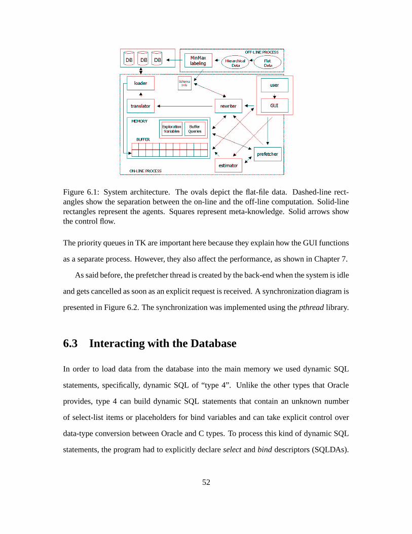
Figure 6.1: System architecture. The ovals depict the flat-file data. Dashed-line rect-angles show the separation between the on-line and the off-line computation. Solid-linerectangles represent the agents. Squares represent meta-knowledge. Solid arrows showthe control flow.

The priority queues in TK are important here because they explain how the GUI functions

as a separate process. However, they also affect the performance, as shown in Chapter 7.

As said before, the prefetcher thread is created by the back-end when the system is idle

and gets cancelled as soon as an explicit request is received. A synchronization diagram is

presented in Figure 6.2. The synchronization was implemented using the pthread library.

6.3 Interacting with the Database

In order to load data from the database into the main memory we used dynamic SQL

statements, specifically, dynamic SQL of “type 4”. Unlike the other types that Oracle

provides, type 4 can build dynamic SQL statements that contain an unknown number

of select-list items or placeholders for bind variables and can take explicit control over

data-type conversion between Oracle and C types. To process this kind of dynamic SQL

statements, the program had to explicitly declare select and bind descriptors (SQLDAs).

52

Figure 6.2: System synchronization. The dashed-line rectangle represents the mainthread. The rectangles on the left hand side of the main thread form the prefetcher thread.The GUI acts as a separate process, due to the priority queues of TK.

A select descriptor holds descriptions of select-list items, and the addresses of output

buffers where the names and values of select-list items are stored. A bind descriptor

holds descriptions of bind variables and indicator variables, and the addresses of input

buffers where the names and values of bind variables and indicator variables are stored.

This solution is required in our system due to the fact that the user can dynamically

change the dataset to be used during the exploration. Thus, the table which is queried

(and implicitly the name and number of the attributes, etc.) changes as well.

53

Chapter 7

Experimental Results

7.1 Experimental Inputs

Performance measurements in systems where human interaction is needed require typi-

cally some way of simulating the users. The main reasons for that is that exactly the same

sequence of operations has to be performed multiple times. User input (also referred to

as user script or input script from now onwards) is a sequences of user operations and

the time specification of when the operations occur. In XmdvTool, the user input is a

sequence of navigation primitives and delays. An example of user script is presented

below:

1000 3 0.0500001200 1 0.1000001400 1 0.1500001600 2 0.200000

The first column contains the time specification, the second the type of the operation and

the third the parameters that the operation requires.

The main goal for our input simulation is to provide “data specificity” and “user speci-

ficity” to the scripts that we generate. In other words the scripts need to show how particu-

54

larities in the data may affect the navigation and also how particularities in user behaviour

(personal preferences) may influence the same. These particularities provide the hints that

we exploit when prefetching.

We simulate the specificity in data by using “hot regions” (Fig. 7.1). Hot regions

are places in the navigation space from where some interesting properties in the data

are visible and where the user will consequently likely examine. Our assumption is that

sooner or later the user will reach those hot regions and thus moving toward them is more

probable. The size and the number of these hot regions as well as the probability of using

them are factors that can vary as we will show in Section 7.2.

Figure 7.1: Hot regions: selections in the navigation space that provide useful insight intothe data.

We also simulate the specificity in the user behaviour. First, we use a probability

factor that gives the likelihood that the user keeps moving in the same direction. This

seems pretty natural given the navigation environment. Each navigation tool (widget in

the GUI) corresponds to a direction. The user will use the same navigation tool for a

while and then change to another one, and so on. Second, we distinguish various classes

of delays that may occur. We differentiate between short delays that occur between two

consecutive events when using the same tool, moderate delays when, for instance, the

user changes the navigation tool and large delays when the user analyzes the data. The

probability value as well as the delay values can be varied as we will show in Section 7.2.

55

Given the factors just described, the user moves pseudo-randomly in our experiments,

i.e., some of the future possible actions are more probable than others, but choosing

among these actions is still performed non-deterministically. The input scripts may af-

fect the system’s performance. Therefore, the results we present further are obtained as

the average of multiple runs in which the scripts are generated with the same parameters.

The approach used to model user navigation may not be the only possible one. Ob-

viously, we feel that our method generates scripts that are close to real ones; however,

further research is needed to validate this assumption.

7.2 Settings

All experiments were conducted on an Alpha v4.0 878 DEC station, running Oracle 8.1.5.

We used C as the host language and embedded SQL statements for accessing the data in

the database.

Throughout all phases of testing we used different types of datasets, both real and

synthetic ones, with always consistent results. However, all experiments we report in this

thesis are based on synthetic data only. We made this choice to avoid the problems caused

by non-homogeneous structures in interpreting the result, since the performance depends

to some degree on the shape of the tree, i.e, the distribution of the nodes in the clustering

tree.

Thus we used complete trees with a constant fan-out (2). The eleven datasets we used

have between 128 (same as IRIS benchmark) and 10 million datapoints, between 8 and

20 dimensions, and between 1,024 (210) and 65,536 216 objects as the maximum number

of points displayed at a time. The datasets named: D1, D2, D3, D128, D1k, D2k, D4k,

D1k10k, D1k100k, D1k1M, D1k10M, had respectively 4096, 65536, 131072, 128, 1024,

2048, 4096, 10000, 100000, 1000000, and 10000000 objects, and a maximum number of

56

displayed objects of 2048, 32768, 65536, 128, 1024, 2048, 4096, 1024, 1024, 1024, and

1024 respectively.

We also varied the user input (number of focus regions, delay factor, “keep direction”

factor) and some system parameters (prefetching strategy, hints to query optimizer, and

size of the data). In all experiments we used navigation scripts containing between 300

and 3000 user operations.

The values we measured during the experiments were: quality, query-based hit ratio,

objects-based hit ratio, and latency. The quality is the number of objects being displayed

during a navigation session. As explained in Chapter 6, the display requests in TK are

queued and served when the system is idle. However, if two display requests refer to the

same widget, the older one is cancelled. This behaviour may result in lost information,

when the display requests are too frequent. This is why we consider the number of objects

being displayed as a measure of the visual quality. The hit ratio is the number of hits over

the total number of items (queries or objects) requested from the back-end. The latency

is the total time, expressed in seconds, in which the user had to wait for her requests to be

served, i.e., the on-line loading time.

7.3 Experiments

Experiment 1: MinMax vs. Recursive. First, we measured the system’s performance

when implementing the structure-based brushes using both the MinMax tree technique

and a direct implementation of the query specification, i.e., a recursive technique. As SQL

does not support recursive views, the recursive technique used an additional attribute to

mark the tuples selected by that time by all previous recursion steps. In both cases we

used the schema described in Chapter 4 and created simple indices on the join attributes

and compound indices on extent and level attributes. Maintaining the indices was not an

57

issue because the trees were static during our experiments. The results of the experiment

are presented in Figures 7.2 – 7.4. As expected, the MinMax method is substantially faster

than the recursive one in all cases. These results show clearly that the application of the

MinMax technique in our system made visual exploration over large datasets practically

feasible, thus accomplishing our ultimate goal.

Figure 7.2: MinMax vs. Recursive.Structure-based brushes for datasetD1.


Experiment 2: Varying brush parameters. In the next three experiments we ana-

lyze the behaviour of the system when the size of the brushes changes. Specifically we

vary the level value, the extent values and the size of the dataset. For these experiments

we use a compound index on�e1 � e2 � L � and a NOCACHE hint for the Oracle’s optimizer.

Since the brushes are implemented as range queries, we expect that the response time will

vary linearly with respect to all these parameters.

Experiment 2a: Varying the level value. In this experiment, the extent values are

constant (0 � 25 � 0 � 75) and the level value vary in two-unit increments. As in a complete

binary tree the number of points increases exponentially (doubles each level), we expected

that the response time would have at most the same growth and thus be linear in the size

of the input. However, as one can see in Fig. 7.5, the linear behaviour can be observed

only for large levels, while for small ones it is almost constant.

Experiment 2b: Varying the extent values. In this experiment, the level value is

58


Figure 7.5: Varying the level value.Functions compared against 2x.Logarithmic y scale.

constant (11 – the leaf level in the smallest dataset) and the extent values varies from�0 � 0 � 0 � 0 � to

�0 � 0 � 1 � 0 � in 0 � 2 increments (captured on the x-axis). The behaviour is again

expected to be linear. This experiment is particularly important since it validates our

assumption that the incremental computing of brushes is needed. Indeed, as shown in

Fig. 7.6, the increase in the response time is linear. Thus the processing time for a level-

based brush is proportionally reduced when computing it incrementally.

Figure 7.6: Varying the extentvalue. Functions compared againstx

�1.

Figure 7.7: Varying the dataset size.Levels 12 and 14 not defined forD1.

Experiment 2c: Varying the size of the dataset. In this experiment we used dataset

D4, having 218 � 262144 tuples. The brush settings are set to values from�0 � 25 � 0 � 75;8 �

to�0 � 25 � 0 � 75;14 � , and the dataset changes from D1 (4096 tuples) to D4 (262144 tuples).

59

The number of nodes doubled from D1 to D2, from D2 to D3, and from D3 to D4 (shown

on the x-axis). However, as one can see in Fig. 7.7, the resulting time is almost constant.

This ensures that our system indeed scales well to large datasets.

Experiment 3: Varying user input. In the next three experiments we analyze the

behaviour of the system when the user input changes. Specifically we vary the size of the

delays between events, the number of the hot regions and the probability parameter that

determines if the current direction is abandoned or not. For these experiments we use the

dataset D1k100k (having a total of 100,000 objects and 1,000 objects in the maximum

active set), and the NOCACHE hint for the Oracle’s optimizer. The results represent the

measurements for both direction (S2) and focus (S3) prefetching strategies, with mini-

mum buffer size (i.e., 1,000 objects in this case).

Figure 7.8: Varying the delays forstrategy S2 and S3. Measured qual-ity.

Figure 7.9: Varying the delays forstrategy S2 and S3. Measured hitratio.

Experiment 3a: Varying the delays. In this experiment we vary the delay factor. Ba-

sically, we multiply the default 1/10–1–5 delays with factors of 1, 2, 5, and 10. Increasing

the delays gives the prefetcher more time. Thus, it is natural that the quality (Fig. 7.8), hit

ratio (both at the object and at the query level) (Fig. 7.9), and latency (Fig. 7.10) improve.

Also, we compare the execution of the direction prefetcher (S2) on multiple data sizes

(D128, D1k, D2k, D4k). There is a tendency for the system to perform better than linear

as soon as it exceeds the short delay region. This is expected given that for short delays

60

Figure 7.10: Varying the delays forstrategy S2 and S3. Measured la-tency.

Figure 7.11: Varying the delays forvarious datasets. Measured quality.

most of the prefetching requests get cancelled.

Figure 7.12: Varying the number ofhot regions. Measured both queryand object hit ratio.

Figure 7.13: Varying the “keep di-rection” factor. Measured queryand object hit ratio.

Experiment 3b: Varying the hot regions. In this experiment we vary the number of

hot regions from 2 to 5. As we expected, the results show that the performance decreases

(Fig. 7.12) when the number of hot regions increases. We present here only the hit ratio

measurements, the latency and the quality are not relevant since the input script had to be

changed from one measurement to another.

Experiment 3c: Varying the “keep direction” parameter. In this experiment we

vary the probability of maintaining the same direction when the current sequence of “in-

terruptible” operations is over. Basically, the probability factor gives the likelihood that a

61

Figure 7.14: Varying the “keep di-rection” factor for various datasets.Measured the hit ratio.

Figure 7.15: Varying prefetchingstrategy. Measured object andquery hit ratio.

user will keep using the same manipulation tool. We use factor values from 0.2 to 0.8, in

increments of 0.2. The obvious tendency is that the higher the factor is, the more accurate

the prediction is. We again measured the hit ratio (Fig. 7.13); the latency and the quality

were irrelevant due to the change of the input scripts. Note that the system uses the same

prediction all the time, which is a probability of 0.6. Also, as part of this experiment, we

vary the size of the data for the direction (S2) strategy (Fig. 7.14). The same tendency is

present.

Experiment 4: Varying system settings. In the next three experiments we analyze

how, given a “typical” user input (suggested by the previous set of experiments), the

performance is influenced by various system settings. We used a user script with three

focus regions, a delay multiplication factor of 2 and a “keep direction” factor of 0.60.

For these experiments we varied the prefetching strategy, the hints to the query optimizer

and the size of the dataset. All of the results were obtained as average of multiple runs

(typically 2 to 4), with different input scripts (but generated with the same parameters).

The measurements for each point on the graphs is the result of the execution of 500

operation scripts.

Experiment 4a: Varying the prefetching strategy. In this experiment we tested the

four prefetcher strategies S0, S1, S2, and S3 against two datasets, namely D1k10k and

62

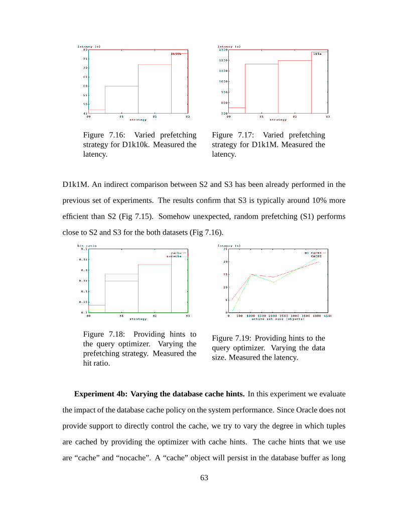
Figure 7.16: Varied prefetchingstrategy for D1k10k. Measured thelatency.

Figure 7.17: Varied prefetchingstrategy for D1k1M. Measured thelatency.

D1k1M. An indirect comparison between S2 and S3 has been already performed in the

previous set of experiments. The results confirm that S3 is typically around 10% more

efficient than S2 (Fig 7.15). Somehow unexpected, random prefetching (S1) performs

close to S2 and S3 for the both datasets (Fig 7.16).

Figure 7.18: Providing hints tothe query optimizer. Varying theprefetching strategy. Measured thehit ratio.

Figure 7.19: Providing hints to thequery optimizer. Varying the datasize. Measured the latency.

Experiment 4b: Varying the database cache hints. In this experiment we evaluate

the impact of the database cache policy on the system performance. Since Oracle does not

provide support to directly control the cache, we try to vary the degree in which tuples

are cached by providing the optimizer with cache hints. The cache hints that we use

are “cache” and “nocache”. A “cache” object will persist in the database buffer as long

63

as possible. A “nocache” object will not be loaded into the buffer. However, nothing

prevents the optimizer to read a “nocache” object from cache, if the object is there. Thus,

the results of these experiments have a higher degree of deviation. In average however

both the hit ratio (Fig 7.18) and the latency (Fig 7.19) improves by about 10%–30%. On

the other hand, the gain of using prefetching is usually at least 150%–200%. It follows

therefore that our technique has a clear advantage over using a commercial cache only. We

varied in this experiment both the prefetch strategy (Fig 7.18) and the data size (Fig 7.19).

Figure 7.20: Varying the dataset.Measured the hit ratio.

Figure 7.21: Varying the dataset.Measured the latency.

Experiment 4c: Varying the dataset size. In this experiment we test the scalability

of our method. We use for this purpose the datasets D1k, D1k10k, D1k100k, D1k1M,

and D1k2M, and all the prefetch strategies S0, S1, S2, and S3. The buffer size is set

to the minimum and the Oracle hints are “nocache”. As one can see, the method scales

better than linear (very similar to a logarithmic curve). It follows that the method is very

appropriate for exploring large datasets, the goal of this thesis.

Discussion. The first set of experiments has demonstrated that recursive processing

of queries is far too expensive to be applied in interactive tools such as XmdvTool. Fur-

thermore, the use of MinMax encoding is shown to make the problem tractable. The

experiments confirmed again the gain of using pre-computed information to support on-

line processing.

64

The second set of experiments has demonstrated that the processing time for a structure-

based brush operation is only proportional to the number of objects being selected and in-

dependent from what brush parameter changed. Thus, the time required for computing a

sequence of brushes is proportional to the sum of the objects in all these selections. These

experiments fully confirmed our approach of computing the structure-based brushes in-

crementally.

The third set of experiments has analyzed how the user input influences the prefetcher

accuracy and thus the system overall efficiency. When there is a clear focus in navigation

or there is enough time between events (requests) the performance improves considerably.

The experiments confirmed the important role of a good predictor.

The fourth set of experiments has analyzed the performance of the system for a fixed

type of user input. The results show that prefetching helps. The system performance

improves significantly compared to the case of using a cache policy only, no matter that

the cache is at the database side or at the application side. Moreover, we have shown that

the system scales better than linearly with respect to the size of the data that is explored.

65

Chapter 8

Conclusions and Future Work

8.1 Conclusions

With the increasing amount of data being accumulated nowadays, the need for visually

exploring large datasets becomes more and more important. A viable way to achieve

scalability in visualization is to integrate visualization applications with database man-

agement systems. Such integrations raise however two kind of problems. First, it requires

the design of an organization of data and a corresponding query mechanism such that all

front-end operations can be translated into efficient database operations. Second, a good

memory management strategy should be employed in order to reduce the overhead of

database accesses and thus make the use of the database transparent to end-users.

This thesis presents a solution that addresses both problems. The approach is be-

ing used to couple XmdvTool4.0, a visualization application for interactive exploration

of multivariate data, with an Oracle8i database management system. Experiments for

assessing the method showed that, despite the recursive nature of the operations at the

interface level, the processing time in our integrated system is only proportional to the

number of objects being selected. Moreover, the system scales linearly with respect to

66

the size of the dataset.

In summary, the main contributions of our approach are:

� The MinMax method was developed in order to improve the applicability of rela-

tional dataset systems for a class of new applications including visualization tools

or CAD/CAM applications. The method provides important advantages over the

traditional recursive approaches when implementing navigation operations on hier-

archical structures due to its fast way to compute the ancestors and the descendents

of the nodes in the tree.

� We implemented the MinMax technique using Oracle 8 and C as a host language

and showed that the MinMax-based queries performed significantly faster than the

equivalent recursive queries. We used this technique to implement the query mech-

anism for XmdvTool [49].

� The caching strategy we employed supports incremental loading of data into the

memory buffer. By hashing the objects from the buffer based on their level value

and by keeping the objects on each level in order, any query containment test against

the data in memory becomes of complexity O�1 � .

� To further reduce the response time in the system, we designed a speculative non-

pure prefetcher that brings data into memory when the system is idle. In order to

ensure efficiency at interruption, the prefetcher uses a cache replacement policy that

combines a low granularity of data (object level) and a “semantic” description of

the content of the buffer.

� Users are synthetically generated for testing the system. Navigation patterns sim-

ulates data specificity as well as user specificity. Moreover, a proper indirection of

the input ensures that exactly the same navigation script can be executed multiple

67

times.

� Experiments showed that the proposed memory management strategy significantly

decreased the latency in the system. The system now scales for datasets of the order

105–107 records.

8.2 Future Work

Directions for further research include both refining the current approach and making it

more general by dropping some of the constraints that we are enforcing now.

The efficiency in the system could be further improved by developing a more accurate

user model. A complex study would need to record and analyze real user input and then

produce classes of patterns that invariantly occur in real navigations. We think that our

model provides a fair approximation of the users. More research is needed to validate this

hypothesis. Once an accurate user model is provided, we could design a more complex

predictor, based on that model. If we confidently know how the patterns look, the task

of extracting the exact parameters from a real navigation script is a tractable statistical

problem.

The system could also be functionally extended by dropping some of the current con-

straints, as for example the “static” assumption. This assumption has two aspects. First,

we might consider dynamic changes of the dataset. It is more and more common to ana-

lyze information that suffers intensive updates during the exploration. Second, we might

dynamically change the tools that we are using during the exploration itself. Dynamic

clustering or dynamic computation of aggregates would be possible for instance.

68

Appendix A

Navigation Operations

A.1 Notation Conventions

In what follows, �� denote a sequence of integers � n1 � n1�

1 �� n2 � . A variable v that

takes all the values from n1 to n2 will be denoted by � �� . A variable v that takes

some values from n1 to n2 (not necessarily all of them) will be denoted by �� .

A.2 Hierarchical Clustering

Let X � � x1 � x2 �� xm � be a set of base data points. Then, P � � P1 � P2 �� Pn � is defined

to be a partition of X iff:

�1

�j

�n : Pj � X (A.1)

�1

�j1 �� j2

�n : Pj1 � Pj2 � /0 (A.2)

n�

j � 1

Pj � X (A.3)

We denote the set X on which partition P is defined by support(P). When using more

69

than one partition, we indicate the partition number by a superscript, e.g.: Pi � � Pi1 � Pi

2 �� Pini

� .

Two partitions Pi1 � � Pi11 � Pi1

2 � �� Pi1ni1

� and Pi2 � � Pi21 � Pi2

2 �� Pi2ni2

� are called nested and

denoted by Pi1 � Pi2 (Pi1 nested in Pi2), iff:

support�Pi1 � � support

�Pi2 � (A.4)

�1

�j2

�ni2 : � 1

�j1

�ni1 : Pi2

j2 � Pi1j1

(A.5)

A hierarchical clustering of X can now be defined as a sequence PX � � P1 � P2 �� Pk �of partitions of X, where:

P1 � X (A.6)

Pk � � � x1 � � � x2 � �� xm � � (A.7)

P1 � P2 � �� Pk (A.8)

A.3 Structure Based Brushes

The hierarchical clustering process, as described in Appendix A.2, results in a tree struc-

ture that is formed on the Pij partitions. Property (A.5) above gives us the parent cluster

(Pi1j1

) for each cluster (Pi2j2

) in the tree. In what follows, the parent of a node Z will be

denoted by θ�Z � . Moreover, for any set of nodes S �� Zt , we will denote by θ

�S � the set

of the parents of S. Thus, θ�S � � � θ

�Zt � .

A structure based brush is basically a set-based function SBB : � 1 �� m � �� 1 �� m � �� k

i � 1 � nij � 1 Pi

j such that SBB�v1 � v2 � � I

�v1 � v2 � � T

�I�v1 � v2 � � � �� T k � 1 �

I�v1 � v2 �� and

where:

1. I�v1 � v2 � � � some j � 1 nk

Pkj � � nk

j � 1 Pkj is the initial selection operator that is applied

to the leaf nodes, and

70

2. T� � some j � 1 ni

Pij � � Pi

j � � � some j � 1 ni � 1Pi � 1

j � � Pi � 1j is a propagation operator

that propagates the selection from one level to its adjacent level. (T i is the notation

for operator T being applied i times.)

Any structure-based brush is consequently fully defined by providing a specification

for the operators I and T.

A.3.1 The ALL Structure Based Brush

In the ALL structure-based brushes, the I operator is defined as:

I�v1 � v2 � � � xv1 �� xv2 � �

nk�

j � 1

Pkj (A.9)

The T operator for an ALL structure-based brush is defined as:

TALL�S � �

some j � 1 ni

Pij � � � Z �

ni�

j � 1

Pi � 1j

�� Y �� ni�

j � 1

Pij �� S : Z � θ

�Y � � (A.10)

A.3.2 The ANY Structure Based Brush

The I operator for the ANY structure-based brushes is identical with the one for the ALL

brushes:

I�v1 � v2 � � � xv1 �� xv2 � �

nk�

j � 1

Pkj (A.11)

The propagation operator T is however different:

TANY�S � �

some j � 1 ni

Pij � � θ

�S � (A.12)

71

A.3.3 The Relational Semantics of Structure-Based Brushes

According to the definitions in Section A.3.1 and Section A.3.2, the propagation operator

corresponds to a division and to a join respectively.

Given a relation R(x, y, ...), where x is a node id and y is the id of the parent of x,

and considering S the initial selection defined by the operator I (same for ALL and ANY

structure-based brushes), the ALL and ANY structure-based brushes define the following

relational operations:

SBBALL � S ��S � R � �

�S � R � R � ��

k � 1�

i � 0

S � R � �� R� �� i times

(A.13)

SBBANY � S ��S � R � �

�S � R � R � ��

k � 1�

i � 0

S � R � �� R� �� i times

(A.14)

72

Appendix B

MinMax Hierarchy Encoding

Let θ�x � be the parent of node x. We define the sets of ancestors anc(x) and descendents

desc(x) of a node x in the hierarchy as follows:

anc�x � � � y

� � node1 � x � node2 �� nodet � 1 � nodet � y :�

i � 2 �� t :

nodei � θ�nodei � 1 � � (B.1)

desc�x � � � y

� � node1 � x � node2 �� nodet � 1 � nodet � y :�

i � 1 �� t � 1 :

nodei � θ�nodei � 1 � � (B.2)

Let now I be the “initial set” and � �a1 � b1 � �

�a2 � b2 � ��

�am � bm � � be the labels of

the leaf nodes in that initial set,�a j � b j � � I � I , a1

�b1

�a2

�b2

� �� am

�bm as

shown in Section 4. A MinMax tree is a labeled tree of the form node�t � � �

aα � t � � bβ � t � � � � t,

where:

α�t � � min � j

�lea f j � desc

�nodet � � (B.3)

β�t � � max � j

�lea f j � desc

�nodet � � (B.4)

� lea fα � t � �� lea fβ � t � � � desc�nodet � (B.5)

73

B.1 Proof of Theorem 1

Theorem: Given a MinMax tree T and two nodes x and y of T whose extent values are�ax1 � ax2 � and

�ay1 � ay2 � respectively, node x is an ancestor of node y if and only if x1

�y1

and y2�

x2.

Proof: We first notice that anc() is a monotonic function. Indeed, relation (B.1) im-

plies that if x � θ�y � then anc

�x �� anc

�y � . Using induction, we further get that:

i f x � anc�y � then anc

�x � � anc

�y � � (B.6)

Analogously, it can be proven that desc() is monotonic, i.e.:

i f y � desc�x �� then desc

�y � � desc

�x � � (B.7)

Implication � : If y � desc�x � then x1

�y1

�y2

�x2.

Indeed, y � desc�x � � � B 7 � ay1 � desc

�y � � desc

�x � � � B 2 � x1

�y1. Similarly, y2

�x2.

Since y1�

y2 is true by construction, we have proven that x1�

y1�

y2�

x2 (q.e.d.).

Implication � : If x1�

y1�

y2�

x2 then y � desc�x � .

We will prove it by contradiction. Let z be the lowest level common ancestor of x and y.

Such a node exists since the root is one common ancestor of x and y. It is also unique

since two nodes on the same level cannot have common descendents (in a tree hierarchy).

Now if x � z or y � z then necessarily x � y � z and x1 � y1�

y2 � x2 (q.e.d.). If x �� z

and y �� z then there exists a child cx � �acx1 � acx2 � of z such that cx = anc(x) and a child

cy � �acy1 � acy2 � of z such that cy = anc(y). cx �� cy follows from the assumption that

z has the lowest level among all the common ancestors. By construction,�cx1 � cx2 � ��

cy1 � cy2 � � /0. However, cx = anc(x) implies that�x1 � x2 � �

�cx1 � cx2 � and cy = anc(y)

implies that�y1 � y2 ��

�cy1 � cy2 � . From the hypothesis

�y1 � y2 ��

�x1 � x2 � and therefore

74

�cx1 � cx2 � �

�cy1 � cy2 � � �

y1 � y2 �� /0 (contradiction) (q.e.d.).


Theorem: Given the brush values vmin and vmax, an ALL structure-based brush gen-

erates the union of all nodes x � �ax1 � ax2 � whose extents are fully contained in the brush

interval�vmin � vmax � , i.e.,

�x1 � x2 ��

�vmin � vmax � .

Proof: Let x � �ax1 � ax2 � be a node and SBB � SBBALL

�v1 � v2 � be an ALL structure-

based brush.

Implication � : If x � SBB then�x1 � x2 � �

�v1 � v2 � .

x � SBB � � 0�

i�

k : x � T i � I �v1 � v2 �� A 10 �

� � y �� T i � 1 �I�v1 � v2 �� : θ

�y � � x �

p � 1 �x � � T i � 1 �

I�v1 � v2 ��

�p � 1 � i � x � � T 0 �

I�v1 � v2 �� I

�v1 � v2 � � ax1 � I

�v1 � v2 � & ax2 �

I�v1 � v2 � � x1 �

�v1 � v2 � & x2 �

�v1 � v2 � � v1

�x1

�x2

�v2 �

�x1 � x2 � �

�v1 � v2 � (q.e.d.).

Implication�

: If�x1 � x2 ��

�v1 � v2 � then x � SBB.

We will prove it by contradiction. If x � Pij then: x �� SBB � � xi � 1 � � ni � 1

j � 1 Pi � 1j �

T k � i � 1 �I�v1 � v2 �� : x � θ

�xi � 1 � � � xi � 2 � � ni � 2

j � 1 Pi � 2j � T k � i � 2 �

I�v1 � v2 �� : xi � 1 � θ

�xi � 2 � �

�� xk � � nkj � 1 Pk

j � I�v1 � v2 � : xk � 1 � θ

�xk � � � xk � �

aa1 � aa2 � � desc�x � : xk �� I

�v1 � v2 � � � T1 �

� �a1 � a2 ��

�x1 � x2 � :

�a1 � a2 ��

�v1 � v2 � �

�x1 � x2 � ��

�v1 � v2 � (contradiction) (q.e.d.).


Theorem: Given the brush values vmin and vmax, an ANY structure-based brush gen-

erates all the nodes x � �ax1 � ax2 � whose intersection with the brush interval

�vmin � vmax �

is not empty, i.e.,�x1 � x2 � �

�vmin � vmax �� /0.

Proof: Let x � �ax1 � ax2 � be a node and SBB � SBBANY

�v1 � v2 � be an ANY structure-

based brush.

75

Implication � : If x � SBB then�x1 � x2 � �

�v1 � v2 � �� /0.

x � SBB � � 0�

i�

k : x � T i � I �v1 � v2 �� xk � i � x � desc

�x � : x � T i � I �

v1 � v2 ��

� xk � i � 1 � desc�x � � x � p � 1 �

xk � i � : xi � 1 � T i � 1 �I�v1 � v2 �� xk � desc

�x � � x �

p � 1 �xk � 1 � : xk � �

aa1 � aa2 � � I�v1 � v2 � � � A 11 � v1

�a1

�a2

�v2. But, xk � �

aa1 � aa2 � �desc

�x � � � T1 � x1

�a1

�a2

�x2 �

�x1 � x2 ��

�v1 � v2 � � �

a1 � a2 �� /0 (q.e.d.).

Implication�

: If�x1 � x2 ��

�v1 � v2 �� /0 then x � SBB.

�x1 � x2 ��

�v1 � v2 �� /0 � � t : t �

�x1 � x2 � �

�v1 � v2 �� t �

�x1 � x2 � & t �

�v1 � v2 � .

t ��x1 � x2 � � at � desc

�x � � � a path � at � xk � xk � 1 � �� xi � x � from at to x such that

xk � 1 � θ�xk � � xk � 2 � θ

�xk � 1 � �� xi � θ

�xi � 1 � .

t ��v1 � v2 � � at � I

�v1 � v2 � � xk � I

�v1 � v2 � � � A 12 � xk � 1 � T

�I�v1 � v2 �� A 12 � xk � 2 �

T 2 �I�v1 � v2 �� A 12 � �� A 12 � xi � T k � i � I �

v1 � v2 �� x � T k � i � I �v1 � v2 �� x � SBB

(q.e.d).

76

Appendix C

Complexity of Memory Operations

For easy reference, buffer operations, as introduced in Chapter 5, are listed again here:

A: Remove old objects. Get the objects with the lowest probability that reside in the

buffer (and further remove them one at a time when more room in the buffer is

needed).

B: Bring new objects. Place an object from the cursor buffer into the memory buffer

(and rehash the buffer entry).

C: Display active set. Get those objects from the buffer that form the active set (and

send them to the graphical interface to have them displayed).

D: Recompute probabilities. Recompute the probabilities of the objects in the buffer

once the active window gets changed (to ensure accurate predictions in the future).

E: Test containment. Test whether the new active set fully resides in the buffer and

get the missing objects (if any) from the support set (when a new request is issued).

77

C.1 Full Size Probability Table

In what follows, the complexity of buffer access operations is presented. The function that

we measured was the number of buffer accesses, i.e., the number of buffer entries that are

visited. For a better understanding, a full version of the probability table is assumed first.

� Remove old objects

Complexity: There are between n � 2 and log n buffer accesses, in average, for

the first element of a single bucket and exactly one buffer access for the following

elements in the bucket list. Since the lists are usually of order n, it follows that

operation A is O�1 � with a good probability.

� Bring new objects

Complexity: There is one operation and a half, on average, for level based rehash-

ing and as many as n � 2 operations in the average for the worst distribution for the

probability based rehashing. The operation is therefore O�n � .

� Display active set

Complexity: There are n buffer accesses in the worst case, but there are no unnec-

essary ones; so that this is optimal. The operation is O�n � .

� Recompute probabilities

Complexity: The objects preserve their level value so no change of the level lists is

needed. However, the probability table needs to be rebuilt, and this takes n�

n2 � 2

operations: n is for deleting the lists (this can be done together with the probability

recomputation step) and n2 � 2 for creating the new ones (it is basically one list

insertion for each object). The operation is O�n2 � .

� Test containment

78

Complexity: Testing is O�1 � , loading the next m objects requires m �

�A�

��B�buffer

accesses, where�X�is the number of buffer accesses for operation X .

C.2 Reduced Probability Table

We now consider the case of a reduced (simplified) probability table. We measure again

the number of buffer accesses. As we shall see, the complexity of some operations de-

creases.

� Remove old objects

Complexity: Same as before.

� Bring new objects

Complexity: There are on average three and a half buffer accesses for rehashing in

this case. The operation is therefore O�1 � .

� Display active set


� Recompute probabilities

Complexity: There are n�

2m buffer accesses. Since m is constant, the operation

is O�n � .

� Test containment


79

Bibliography

[1] D. Andrews. Plots of high dimensional data. Biometrics, Vol. 28, p. 125-36, 1972.

[2] J.-L. Baer and G. R. Sager. Dynamic improvement of locality in virtual memorysystems. IEEE Transactions on Software Engineering, 2(2):137, June 1976.

[3] A. Becker and S. Cleveland. Brushing scatterplots. Technometrics, Vol 29(2), p.127-142, 1987.

[4] D. Calvanese, G. D. Giacomo, and M. Lenzerini. On the decidability of querycontainment under constraints. In Proc of the Seventeenth ACM SIGACT-SIGMOD-SIGART Symp on Princ of Database Systems, Seattle, Washington, pages 149–158.ACM Press, 1998.

[5] P. Cao, E. W. Felten, A. R. Karlin, and K. Li. A study of integrated prefetching andcaching strategies. Technical Report TR-479-94, Princeton University, ComputerScience Department, Dec. 1994.

[6] C. Chekuri and A. Rajaraman. Conjunctive query containment revisited. In F. N.Afrati and P. Kolaitis, editors, Database Theory - ICDT ’97, 6th International Con-ference, Delphi, Greece, volume 1186 of Lecture Notes in Computer Science, pages56–70. Springer, 1997.

[7] P. Ciaccia, D. Maio, and P. Tiberio. A method for hierarchy processing in relationalsystems. Information Systems, 14(2):93–105, 1989.

[8] W. Cleveland and M. McGill. Dynamic Graphics for Statistics. Wadsworth, Inc.,1988.

[9] G. P. Copeland, S. Khoshafian, M. G. Smith, and P. Valduriez. Buffering schemesfor permanent data. In Proc of the Second Intl Conf on Data Engineering, Feb 5-7,1986, Los Angeles, Cal, USA, pages 214–221, 1986.

[10] T. H. Cormen, C. E. Leiserson, and R. L. Rivest. Introduction to algorithms. MITPress and McGraw-Hill Book Company, 6th edition, 1992.

[11] K. M. Curewitz, P. Krishnan, and J. S. Vitter. Practical prefetching via data com-pression. In Proc of the 1993 ACM SIGMOD Intl Conf on Management of Data,Washington, D.C., May 26-28, 1993, pages 257–266. ACM Press, 1993.

80

[12] S. Dar, M. J. Franklin, B. T. Jonsson, D. Srivastava, and M. Tan. Semantic datacaching and replacement. In Proc of 22th Intl Conf on Very Large Data Bases, Sept3-6, 1996, Mumbai (Bombay), India, pages 330–341. Morgan Kaufmann, 1996.

[13] M. Derthick, J. Harrison, A. Moore, and S. Roth. Efficient multi-object dynamicquery histograms. Proc. of Information Visualization, pages 58–64, Oct. 1999.

[14] S. Feiner and C. Beshers. Worlds within worlds: Metaphors for exploring n-dimensional virtual worlds. Proc. UIST’90, p. 76-83, 1990.

[15] D. Florescu, A. Levy, D. Suciu, and K. Yagoub. Run-time management of dataintensive web-sites. Technical report, Inria, Institut National de Recherche en Infor-matique et en Automatique, 1999.

[16] Y. H. Fua, M. O. Ward, and E. A. Rundensteiner. Hierarchical parallel coordinatesfor exploration of large datasets. IEEE Proc. of Visualization, pages 43–50, Oct.1999.

[17] Y. H. Fua, M. O. Ward, and E. A. Rundensteiner. Navigating hierarchies withstructure-based brushes. Proc. of Information Visualization, pages 58–64, Oct. 1999.

[18] J. Haslett, R. Bradley, P. Craig, A. Unwin, and G. Wills. Dynamic graphics forexploring spatial data with application to locating global and local anomalies. Sta-tistical Computing 45(3), p. 234-42, 1991, 1991.

[19] S. Hibino and E. A. Rundensteiner. Processing incremental multidimensional rangequeries in a direct manipulation visual query. In Proc of the Fourteenth Intl Conf onData Engineering, Orlando, Florida, USA, pages 458–465, 1998.

[20] S. Hibino and E. Rundersteiner. User interface evaluation of a direct manipula-tion temporal visual query language. In Proc of The Fifth ACM Intl MultimediaConf (MULTIMEDIA ’97), pages 99–108, New York/Reading, Nov. 1998. ACMPress/Addison-Wesley.

[21] Y. Ioannidis. Dynamic information visualization. SIGMOD Record (ACM SpecialInterest Group on Management of Data), 25(4):16–16, Dec. 1996.

[22] C. Jeong and A. Pang. Reconfigurable disc trees for visualizing large hierarchicalinformation space. Proc. of Information Visualization ’98, p. 19-25, 1998.

[23] D. Joseph and D. Grunwald. Prefetching using Markov predictors. In Proc of the24th Annual Intl Symposium on Computer Architecture (ISCA-97), Computer Ar-chitecture News, pages 252–263, New York, June 1997. ACM Press.

[24] S. Kaushik and E. A. Rundensteiner. SVIQUEL: A spatial visual query and explo-ration language. Lecture Notes in Computer Science, 1460, 1998.

81

[25] A. M. Keller and J. Basu. A predicate-based caching scheme for client-serverdatabase architectures. VLDB Journal, 5(1):35–47, 1996.

[26] T. Kohonen. The self-organizing map. Proc. of IEEE, p. 1464-80, 1978.

[27] Y. Leung and M. Apperley. A review and taxonomy of distortion-oriented presenta-tion techniques. ACM Transactions on Computer-Human Interaction Vol. 1(2), June1994, p. 126-160, 1994.

[28] M. Livny, R. Ramakrishnan, K. S. Beyer, G. Chen, D. Donjerkovic, S. Lawande,J. Myllymaki, and R. K. Wenger. DEVise: Integrated querying and visualizationof large datasets. In Proc ACM SIGMOD Intl Conf on Management of Data, May13-15, 1997, Tucson, Arizona, USA, pages 301–312. ACM Press, 1997.

[29] A. Martin and M. Ward. High dimensional brushing for interactive exploration ofmultivariate data. Proc. of Visualization ’95, p. 271-8, 1995.

[30] A. Mead. Review of the development of multidimensional scaling methods. TheStatistician, Vol. 33, p. 27-35, 1992.

[31] X. Qian. Query folding. In S. Y. W. Su, editor, Proceedings of the Twelfth In-ternational Conference on Data Engineering, February 26 - March 1, 1996, NewOrleans, Louisiana, pages 48–55. IEEE Computer Society, 1996.

[32] G. Robertson, J. Mackinlay, and S. Card. Cone trees: Animated 3d visualizationof hierarchical information. Proc. of Computer-Human Interaction ’91, p. 189-194,1991.

[33] N. Roussopoulos, C.-M. Chen, S. Kelley, A. Delis, and Y. Papakonstantinou. TheADMS project: View R us. Data Engineering Bulletin, 18(2):19–28, 1995.

[34] P. G. Selfridge, D. Srivastava, and L. O. Wilson. Idea: Interactive data explorationand analysis. In Proc of the 1996 ACM SIGMOD Intl Conf on Management of Data,Montreal, Quebec, Canada, June 4-6, 1996, pages 24–34. ACM Press, 1996.

[35] L. D. Shapiro. Join processing in database systems with large main memories. ACMTransactions on Database Systems, 11(3):239–264, 1986.

[36] E. J. Shekita and M. J. Carey. A performance evaluation of pointer-based joins. InProc of the 1990 ACM SIGMOD Intl Conf on Management of Data, Atlantic City,NJ, May 23-25, 1990, pages 300–311. ACM Press, 1990.

[37] B. Shneiderman. Tree visualization with tree-maps: A 2d space-filling approach.ACM Transactions on Graphics, Jan. 1992, 1992.

[38] M. Stonebraker. Inclusion of new types in relational data base systems. In Proc ofthe Intl Conf on Data Engineering, pages 262–269, Los Angeles, CA, Feb. 1986.IEEE Computer Society, IEEE Computer Society Press.

82

[39] M. Stonebraker, J. Chen, N. Nathan, C. Paxson, and J. Wu. Tioga: Providing datamanagement support for scientific visualization applications. In 19th Intl Conf onVery Large Data Bases, 1993, Dublin, Ireland, pages 25–38. Morgan Kaufmann,1993.

[40] I. D. Stroe, E. A. Rundensteiner, and M. O. Ward. Minmax trees: Efficient rela-tional operation support for hierarchy data exploration. Technical Report TR-99-37,Worcester Polytechnic Institute, Computer Science Department, 1999.

[41] I. D. Stroe, E. A. Rundensteiner, and M. O. Ward. Scalable visual hierarchy explo-ration. In Database and Expert Systems Applications, Greenwich, UK, Sept. 2000.to appear.

[42] P. Sulatycke and K. Ghose. A fast multithreaded out-of-core visualization technique.In 13th Intl Parallel Processing Symposium and 10th Symposium on Parallel andDistributed Processing, Apr. 1999.

[43] E. Tanin, R. Beigel, and B. Shneiderman. Incremental data structures and algorithmsfor dynamic query interfaces. ACM Special Interest Group on Management of Data,25(4), Dec. 1996.

[44] J. Teuhola. Path signatures: A way to speed up recursion in relational databases.IEEE Transactions on Knowledge and Data Engineering, 8(3):446–454, June 1996.

[45] P. Valduriez. Join indices. ACM Transactions on Database Systems, 12(2):218–246,1987.

[46] P. Valduriez, S. Khoshafian, and G. P. Copeland. Implementation techniques ofcomplex objects. In VLDB’86 Twelfth Intl Conf on Very Large Data Bases, August25-28, 1986, Kyoto, Japan, Proc, pages 101–110. Morgan Kaufmann, 1986.

[47] M. O. Ward. Xmdvtool: Integrating multiple methods for visualizing multivariatedata. Proc. of Visualization, pages 326–333, 1994.

[48] G. Wills. Selection: 524,288 ways to say this is interesting. Proc. of InformationVisualization ’96, p. 54-9, 1996.

[49] Xmdvtool home page. http://davis.wpi.edu/˜xmdv.

[50] T. Zhang, R. Ramakrishnan, and M. Livny. Birch: an efficient data clusteringmethod for very large databases. SIGMOD Record, vol.25(2), p. 103-14, pages103–114, June 1996.

83

Documents

Scalable Visual Hierarchy Exploration - Worcester …davis.wpi.edu/~xmdv/docs/stroe_msthesis.pdf · · 2003-04-211.1 Caching and Prefetching for Large-Scale Visualization ... without