Clutter Reduction in Multi-Dimensional Data Visualization Using Dimension

Reordering∗

Wei Peng, Matthew O. Ward and Elke A. Rundensteiner

Computer Science Department, Worcester Polytechnic Institute, Worcester, MA 01609

{debbie,matt,rundenst}@cs.wpi.edu

ABSTRACT

Visual clutter denotes a disordered collection of graphical entities ininformation visualization. Clutter can obscure the structure presentin the data. Even in a small dataset, clutter can make it hard for theviewer to find patterns, relationships and structure.

In this paper, we define visual clutter as any aspect of the vi-sualization that interferes with the viewer’s understanding of thedata, and present the concept of clutter-based dimension reorder-ing. Dimension order is an attribute that can significantly affect avisualization’s expressiveness. By varying the dimension order in adisplay, it is possible to reduce clutter without reducing informationcontent or modifying the data in any way.

Clutter reduction is a display-dependent task. In this paper, wefollow a three-step procedure for four different visualization tech-niques. For each display technique, first, we determine what consti-tutes clutter in terms of display properties; then we design a metricto measure visual clutter in this display; finally we search for anorder that minimizes the clutter in a display.

CR Categories: H.5.2 [Information Interfaces and Presentation]:User Interfaces—Graphical user interfaces I.5.3 [Pattern Recogni-tion]: Clustering—Similarity Measures

Keywords: Multidimensional visualization, dimension order, vi-sual clutter, visual structure.

1 INTRODUCTION

Visualization is the graphical presentation of information with thegoal of helping the user gain a qualitative understanding of the in-formation. A good visualization clearly reveals structure within thedata and thus can help the viewer to better identify patterns and de-tect outliers. Clutter, on the other hand, is characterized by crowdedand disordered visual entities that obscure the structure in visualdisplays. In other words, clutter is the opposite of structure; it cor-responds to all the factors that interfere with the process of findingstructures. Clutter is certainly undesirable since it hinders view-ers’ understanding of the content of the displays. However, whenthe dimensions or number of data items grow high, it is inevitablefor displays to exhibit some clutter, no matter what visualizationmethod is used.

To address this problem, many clutter reduction techniques havebeen proposed, such as multi-resolution approaches [23, 7, 24], di-mensionality reduction approaches [9, 12, 22, 11], and distortionapproaches [16, 14]. However, they either sacrifice the integrity ofthe data or fail to generate an unbiased representation of the data.In order to complement these approaches by reducing clutter in tra-ditional visualization techniques while retaining the information in

∗This work was supported under NSF grant IIS-0119276.

the display, we propose a clutter reduction technique using dimen-sion reordering.

In many multivariate visualization techniques, such as parallelcoordinates [8, 21], glyphs [1, 15], scatterplot matrices [3] andpixel-oriented methods [10], dimensions are positioned in someone- or two-dimensional arrangement on the screen [25]. Giventhe 2-D nature of this medium, some ordering or organization ofthe dimensions must be assumed. This organization can have amajor impact on the expressiveness of the visualization. Differ-ent orderings of dimensions can reveal different aspects of the dataand affect the perceived clutter and structure in the display. Thuscompletely different conclusions may be drawn based on each dis-play. Unfortunately, in many existing visualization systems that en-compass these techniques, dimensions are usually ordered withoutmuch care. In fact, dimensions are often displayed by the defaultorder in the original dataset. Manual dimension ordering is avail-able in some systems. For example, Polaris [18] allows users tomanually select and order the dimensions to be mapped to the dis-play. Similarly, in XmdvTool [25], users can manually change theorder of dimensions from a reconfigurable list of dimensions. How-ever, the exhaustive search for the best ordering is tedious even for amodest number of dimensions. Therefore, automatic clutter-baseddimension ordering techniques that would remedy this shortcomingof current tools are needed.

Clutter reduction is a visualization-dependent task because visu-alization techniques vary largely from one to another. The basicgoal of this paper is to present clutter measuring and reduction ap-proaches for several of the most popular visualization techniques,namely parallel coordinates [8, 21], scatterplot matrices [3], starglyphs [17], and dimensional stacking [13]. Although we onlychose these visualization techniques to experiment with, there aremany more traditional visualization techniques that could benefitfrom this concept.

In order to automate the dimension reordering process for a dis-play, we are concerned with three issues: (1) determining the wayclutter manifests itself in the display, (2) designing a metric to mea-sure visual clutter, and (3) arranging the dimensions for the purposeof clutter reduction. The solutions we provide are specifically tunedto each individual visualization technique. In some techniques, wereduce the level of noise in the display; in other cases we increasethe number of clusters. For each technique we will follow a simi-lar procedure. First we determine the visual characteristics that wewould label as clutter. Next, we carefully define a metric for mea-suring clutter. Then we find the dimension order that minimizes theclutter in a display.

The remainder of this paper is organized as follows. Section 2provides a review of related work. Sections 3, 4, 5, and 6 discussthe clutter definitions and measures for four different visualizationtechniques respectively. In Section 7, algorithms for reordering arepresented. Conclusions and future work are presented in Section 8.

2 RELATED WORK

Many approaches have been proposed to overcome the clutter prob-lem. Distortion [16, 14] is a widely used technique for clutter reduc-

tion. In visualizations supporting distortion-oriented techniques,the interesting portion of the data is given more display space. Theproblem with this technique is that the uninteresting subset of thedata is squeezed into a small area, making it difficult for the viewerto fully understand it. Multi-resolution approaches [23, 7, 24] areused to group the data into hierarchies and display them at a desiredlevel of detail. These approaches do not retain all the information inthe data, since many details will be filtered out at low resolutions.

High dimensionality is another source of clutter. Many ap-proaches exist for dimension reduction. Principal ComponentAnalysis [9], Multi-dimensional Scaling [12, 22], and Self Orga-nizing Maps [11] are popular dimensionality reduction techniquesused in data and information visualization. Yang et al. [27] pro-posed a visual hierarchical dimension reduction technique that cre-ates meaningful lower dimensional spaces with representative di-mensions from the original data space instead of generating newdimensions. These techniques generate a lower dimensional sub-space to reduce clutter but some information in the original dataspace is also lost.

In information visualization, many visual factors can be orderedto enhance the displays. Friendly et al. [6] designed a generalframework for ordering information, including arrangement of vari-ables, according to the desired effects or trends. Dimension order-ing has also been studied in [2, 26]. Ankerst et al. [2] proposed amethod to arrange dimensions according to their similarities so thatsimilar ones are adjacent to each other. They used Euclidean dis-tance as the similarity measure, proved that the arrangement prob-lem is NP-complete, and applied heuristic algorithms to search forthe optimal order. Yang et al. [26] imposed a hierarchical struc-ture over the dimensions themselves, grouping a large number ofdimensions into a hierarchy so that the complexity of the order-ing problem is reduced. User interactions are then supported tomake it practical for users to actively decide on dimension reduc-tion and ordering in the visualization process. However, in thoseapproaches, dimensions are reordered according to only one partic-ular measure, the similarity between dimensions. In many visual-ization techniques, the overall clutter in the display is not alwaysrelated to similarity between dimensions. Ordering dimensions ac-cording to the best correlation does not guarantee the least clutter.But their idea of using dimension ordering inspired our work ofordering dimensions to improve visualization quality.

3 PARALLEL COORDINATES

Parallel coordinates is a popular multivariate visualization tech-nique [8, 21]. In this method, each dimension corresponds to anaxis, and the N axes are organized as uniformly spaced vertical orhorizontal lines. A data element in an N-dimensional space mani-fests itself as a connected set of points, one on each axis. Thus apolyline is generated for representing one data point.

3.1 Clutter Analysis of Parallel Coordinates

In the parallel coordinates display, as the axes order is changed, thepolylines representing data points take on very distinct shapes. InFigures 1 and 2, the two displays depict the same dataset with dif-ferent dimension orders. As can be seen in the figure, a parallelcoordinates display makes inter-dimensional relationships betweenneighboring dimensions easy to see, but does not disclose relation-ships between non-adjacent dimensions. In a full display of parallelcoordinates without sampling, filtering or multi-resolution process-ing, if polylines between two dimensions can be naturally groupedinto a set of clusters, the user will likely find it easier to comprehendthe relationship between them. Instead, if there are many lines thatdon’t belong to any cluster, the space between the two dimensionscan be very cluttered. These polylines don’t help the viewer to find

patterns and discover relationships. Those data points that don’tbelong to any cluster are called outliers. It is true that one of theadvantages of parallel coordinates visualization is to help find out-liers, but in our case, a lot of outliers between a pair of dimensionsindicates that there is little relationship between the two of them.Since our goal is to disclose more relationships and patterns be-tween dimensions, we want to minimize the impact from outliers,in other words, we carefully order the dimensions to avoid them.

3.2 Clutter Measure in Parallel Coordinates

3.2.1 Defining and Computing Clutter

Due to the fact that outliers often obscure structure and thus con-fuse the user, clutter in parallel coordinates can be defined as theproportion of outliers against the total number of data points. Toreduce clutter in this technique, our task is to rearrange the dimen-sions to minimize the outliers between neighboring dimensions. Tocalculate the score for a given dimension order, we first count thetotal number of outliers between neighboring dimensions, Soutlier.If there are n dimensions, the number of neighboring pairs for agiven order is n− 1. The average outlier number between dimen-sions is defined to be Savg = Soutlier/(n− 1). Let Stotal denote thetotal number of data points. The clutter C , defined as the proportionof outliers, can then be calculated as follows:

C = Savg/Stotal =Soutlier

n−1

Stotal

(1)

Since n−1 and Stotal are both fixed for a given dataset, dimen-sion orders that reduce the total number of outliers also reduce clut-ter in the display according to our notion of clutter.

Now we are faced with the problem of how to decide if a dataitem is within a cluster or is an outlier. Since we have restrictedthe notion of clutter to the number of outliers within neighboringpairs of dimensions, we can use the normalized Euclidean distancesbetween data points to measure their closeness. If a data point doesnot have any neighbor whose distance to it is less than thresholdt, we treat it as an outlier. In this way, we are able to find all thedata points that don’t have any neighbors within the distance t inthe specified two-dimensional space. If the number of data pointsis m, this is done in O(m2) time. We do this for every pair of the ndimensions and store the outlier numbers in a outlier matrix M. Thetotal time for building this matrix is O(m2n2). Given a dimensionorder, we can then decide the clutter in the display by adding upoutlier numbers between neighboring dimensions.

Instead of letting the user specify the threshold, we could havedecided it based on the dataset, or develop algorithms that don’tinvolve thresholds. However, since we want to give the user moreflexibility and interaction when ordering the dimensions, we be-lieve that allowing the user to decide the thresholds of cluster widthis preferable. Thus the threshold here and those in the followingchapters all can be user-defined, though with a fixed default value.

3.2.2 The Optimal Dimension Order

Optimal dimension ordering would be to select the one dimensionorder that minimizes visual clutter. In a given dimension order,adding up outlier numbers between neighboring dimensions takesO(n) time. Since the optimal dimension ordering algorithm is anexhaustive search algorithm with O(n!) time, the search time in-volved is O(n∗n!).

3.3 Example

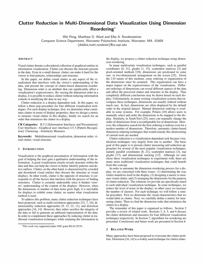
Figures 1 and 2 both represent the Cars dataset. In Figure 1 the datais displayed with the default dimension ordering. Figure 2 displays

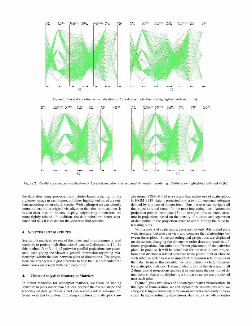
Figure 1: Parallel coordinates visualization of Cars dataset. Outliers are highlighted with red in (b).

Figure 2: Parallel coordinates visualization of Cars dataset after clutter-based dimension reordering. Outliers are highlighted with red in (b).

the data after being processed with clutter-based ordering. In therightmost image in each figure, polylines highlighted in red are out-liers according to our clutter metric. With a glimpse we can identifymore outliers in the original visualization than the improved one. Itis also clear that, in the new display, neighboring dimensions aremore tightly related. In addition, the data points are better sepa-rated and thus it is easier for the viewer to find patterns.

4 SCATTERPLOT MATRICES

Scatterplot matrices are one of the oldest and most commonly usedmethods to project high dimensional data to 2-dimensions [1]. Inthis method, N ∗ (N −1)/2 pairwise parallel projections are gener-ated, each giving the viewer a general impression regarding rela-tionships within the data between pairs of dimensions. The projec-tions are arranged in a grid structure to help the user remember thedimensions associated with each projection.

4.1 Clutter Analysis in Scatterplot Matrices

In clutter reduction for scatterplot matrices, we focus on findingstructure in plots rather than outliers, because the overall shape andtendency of data points in a plot can reveal a lot of information.Some work has been done in finding structures in scatterplot visu-

alizations. PRIM-9 [19] is a system that makes use of scatterplots.In PRIM-9 [19] data is projected onto a two-dimensional subspacedefined by any pair of dimensions. Thus the user can navigate allthe projections and search for the most interesting ones. Automaticprojection pursuit techniques [5] utilize algorithms to detect struc-ture in projections based on the density of clusters and separationof data points in the projection space to aid in finding the most in-teresting plots.

With a matrix of scatterplots, users are not only able to find plotswith structure, but also can view and compare the relationships be-tween these plots. Since all orthogonal projections are displayedon the screen, changing the dimension order does not result in dif-ferent projections, but rather a different placement of the pairwiseplots. In practice, it will be beneficial for the user to have projec-tions that disclose a related structure to be placed next or close toeach other in order to reveal important dimension relationships inthe data. To make this possible, we have defined a clutter measurefor scatterplot matrices. The main idea is to find the structure in all2-dimensional projections and use it to determine the position of di-mensions so that plots displaying a similar structure are positionednear each other.

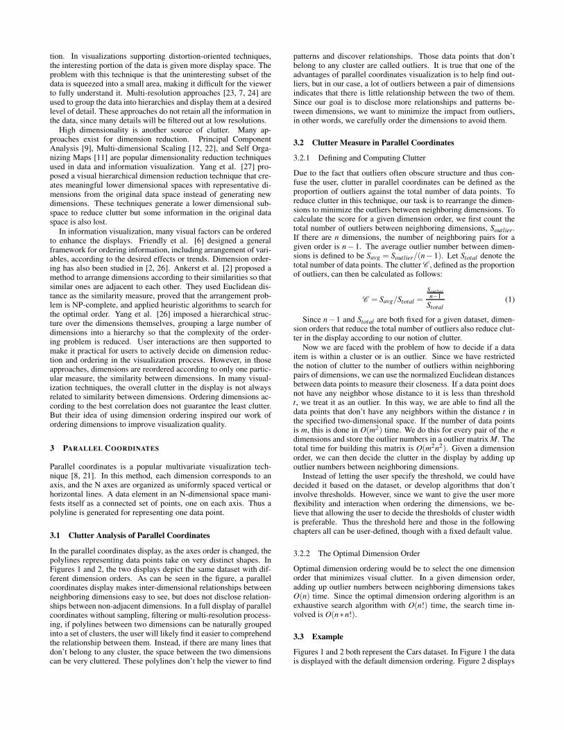
Figure 3 gives two views of a scatterplot matrix visualization. Inthis type of visualization, we can separate the dimensions into twocategories: high-cardinality dimensions and low-cardinality dimen-sions. In high-cardinality dimensions, data values are often contin-

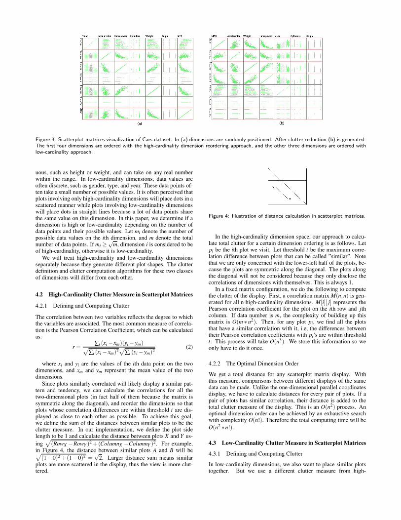
Figure 3: Scatterplot matrices visualization of Cars dataset. In (a) dimensions are randomly positioned. After clutter reduction (b) is generated.The first four dimensions are ordered with the high-cardinality dimension reordering approach, and the other three dimensions are ordered withlow-cardinality approach.

uous, such as height or weight, and can take on any real numberwithin the range. In low-cardinality dimensions, data values areoften discrete, such as gender, type, and year. These data points of-ten take a small number of possible values. It is often perceived thatplots involving only high-cardinality dimensions will place dots in ascattered manner while plots involving low-cardinality dimensionswill place dots in straight lines because a lot of data points sharethe same value on this dimension. In this paper, we determine if adimension is high or low-cardinality depending on the number ofdata points and their possible values. Let mi denote the number ofpossible data values on the ith dimension, and m denote the totalnumber of data points. If mi ≥

√m, dimension i is considered to be

of high-cardinality, otherwise it is low-cardinality.

We will treat high-cardinality and low-cardinality dimensionsseparately because they generate different plot shapes. The clutterdefinition and clutter computation algorithms for these two classesof dimensions will differ from each other.

4.2 High-Cardinality Clutter Measure in Scatterplot Matrices

4.2.1 Defining and Computing Clutter

The correlation between two variables reflects the degree to whichthe variables are associated. The most common measure of correla-tion is the Pearson Correlation Coefficient, which can be calculatedas:

r =∑i (xi −xm)(yi −ym)

√

∑i (xi −xm)2√

∑i (yi −ym)2(2)

where xi and yi are the values of the ith data point on the twodimensions, and xm and ym represent the mean value of the twodimensions.

Since plots similarly correlated will likely display a similar pat-tern and tendency, we can calculate the correlations for all thetwo-dimensional plots (in fact half of them because the matrix issymmetric along the diagonal), and reorder the dimensions so thatplots whose correlation differences are within threshold t are dis-played as close to each other as possible. To achieve this goal,we define the sum of the distances between similar plots to be theclutter measure. In our implementation, we define the plot sidelength to be 1 and calculate the distance between plots X and Y us-

ing√

(RowX −RowY )2 +(ColumnX −ColumnY )2. For example,in Figure 4, the distance between similar plots A and B will be√

(1−0)2 +(1−0)2 =√

2. Larger distance sum means similarplots are more scattered in the display, thus the view is more clut-tered.

Figure 4: Illustration of distance calculation in scatterplot matrices.

In the high-cardinality dimension space, our approach to calcu-late total clutter for a certain dimension ordering is as follows. Letpi be the ith plot we visit. Let threshold t be the maximum corre-lation difference between plots that can be called ”similar”. Notethat we are only concerned with the lower-left half of the plots, be-cause the plots are symmetric along the diagonal. The plots alongthe diagonal will not be considered because they only disclose thecorrelations of dimensions with themselves. This is always 1.

In a fixed matrix configuration, we do the following to computethe clutter of the display. First, a correlation matrix M(n,n) is gen-erated for all n high-cardinality dimensions. M[i][ j] represents thePearson correlation coefficient for the plot on the ith row and jthcolumn. If data number is m, the complexity of building up thismatrix is O(m ∗ n2). Then, for any plot pi, we find all the plotsthat have a similar correlation with it, i.e, the differences betweentheir Pearson correlation coefficients with pi’s are within thresholdt. This process will take O(n3). We store this information so weonly have to do it once.

4.2.2 The Optimal Dimension Order

We get a total distance for any scatterplot matrix display. Withthis measure, comparisons between different displays of the samedata can be made. Unlike the one-dimensional parallel coordinatesdisplay, we have to calculate distances for every pair of plots. If apair of plots has similar correlation, their distance is added to thetotal clutter measure of the display. This is an O(n2) process. Anoptimal dimension order can be achieved by an exhaustive searchwith complexity O(n!). Therefore the total computing time will be

O(n2 ∗n!).

4.3 Low-Cardinality Clutter Measure in Scatterplot Matrices

4.3.1 Defining and Computing Clutter

In low-cardinality dimensions, we also want to place similar plotstogether. But we use a different clutter measure from high-

cardinality dimensions.For plots with low-cardinality dimensions, the higher the car-

dinality, the more crowded the plot seems to be. Therefore, in-stead of navigating all dimension orders and searching for the bestone, we will order these dimensions according to their cardinalities.Dimensions with higher cardinality are positioned before lower-cardinality dimensions. In this way, plots with similar density areplaced near each other. This satisfies our purpose for clutter reduc-tion. The dot density of plots will appear to decrease gradually,resulting in less clutter, or more perceived order, in the view.

4.3.2 The Optimal Dimension Order

With low-cardinality dimensions, the dimension reordering can beenvisioned as a sorting problem. With a quick sort algorithm, it canbe achieved within O(n∗ log n) time.

4.4 Example

From Figure 3 we notice that plots generated by two high-cardinality dimensions are very different in pattern with plots in-volving one or two low-cardinality dimensions. We believe thatseparating the high and low-cardinality dimensions from each otheris useful in identifying similar low-cardinality dimensions and find-ing similar plots in the high-cardinality dimension subspace.

5 STAR GLYPHS

5.1 Clutter Analysis in Star Glyphs

A glyph is a representation of a data element that maps data valuesto various geometric and color attributes of graphical primitives orsymbols [15]. XmdvTool [25] uses star glyphs [17] as one of itsfour visualization approaches. In this technique, each data elementoccupies one portion of the display window. Data values control thelength of rays emanating from a central point. The rays are joinedby a polyline drawn around the outside of the rays to form a closedpolygon.

In star glyph visualization, each glyph represents a differentdata point. With dimensions ordered differently, the glyph’s shapevaries. Since glyphs are stand-alone graphical entities, we considerreducing clutter here as to make those single data points overallseem more structured. Alternatively we could have focused onglyph placement as a means of reducing clutter. Gestalt Laws arerobust rules of pattern perception [20]. They state that similarityand symmetry are two factors that help viewers see patterns in thevisual display. We call a glyph well structured if its rays are ar-ranged so that they have similar length to their neighbors and arewell balanced along some axis. In our approach, we define mono-tonicity and symmetry as our measures of structure for glyphs.Therefore user can find monotonic structure, symmetric structure,or a combination of the two in the data.

Let’s take monotonicity+symmetry for example. In a perfectlystructured glyph:

• Neighboring rays have similar lengths.

• The lengths of rays are ordered in a monotonically increasingor decreasing manner on both sides of an axis.

• Rays of similar lengths are positioned symmetrically alongeither a horizontal or vertical axis.

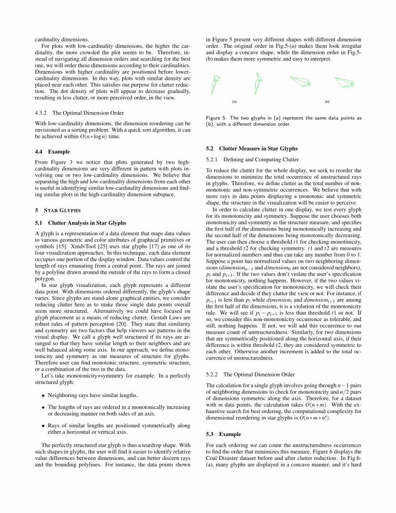
The perfectly structured star glyph is thus a teardrop shape. Withsuch shapes in glyphs, the user will find it easier to identify relativevalue differences between dimensions, and can better discern raysand the bounding polylines. For instance, the data points shown

in Figure 5 present very different shapes with different dimensionorder. The original order in Fig.5-(a) makes them look irregularand display a concave shape, while the dimension order in Fig.5-(b) makes them more symmetric and easy to interpret.

Figure 5: The two glyphs in (a) represent the same data points as(b), with a different dimension order.

5.2 Clutter Measure in Star Glyphs

5.2.1 Defining and Computing Clutter

To reduce the clutter for the whole display, we seek to reorder thedimensions to minimize the total occurrence of unstructured raysin glyphs. Therefore, we define clutter as the total number of non-monotonic and non-symmetric occurrences. We believe that withmore rays in data points displaying a monotonic and symmetricshape, the structure in the visualization will be easier to perceive.

In order to calculate clutter in one display, we test every glyphfor its monotonicity and symmetry. Suppose the user chooses bothmonotonicity and symmetry as the structure measure, and specifiesthe first half of the dimensions being monotonically increasing andthe second half of the dimensions being monotonically decreasing.The user can then choose a threshold t1 for checking monotinicity,and a threshold t2 for checking symmetry. t1 and t2 are measuresfor normalized numbers and thus can take any number from 0 to 1.Suppose a point has normalized values on two neighboring dimen-sions (dimensionn−1 and dimension0 are not considered neighbors),pi and pi+1. If the two values don’t violate the user’s specificationfor monotonicity, nothing happens. However, if the two values vi-olate the user’s specification for monotonicity, we will check theirdifference and decide if they clutter the view or not. For instance, ifpi+1 is less than pi while dimensioni and dimensioni+1 are amongthe first half of the dimensions, it is a violation of the monotonicityrule. We will see if pi − pi+1 is less than threshold t1 or not. Ifso, we consider this non-monotonicity occurrence as tolerable, andstill, nothing happens. If not, we will add this occurrence to ourmeasure count of unstructuredness. Similarly, for two dimensionsthat are symmetrically positioned along the horizontal axis, if theirdifference is within threshold t2, they are considered symmetric toeach other. Otherwise another increment is added to the total oc-currence of unstructuredness.

5.2.2 The Optimal Dimension Order

The calculation for a single glyph involves going through n−1 pairsof neighboring dimensions to check for monotonicity and n/2 pairsof dimensions symmetric along the axis. Therefore, for a datasetwith m data points, the calculation takes O(n ∗m). With the ex-haustive search for best ordering, the computational complexity fordimensional reordering in star glyphs is O(n∗m∗n!).

5.3 Example

For each ordering we can count the unstructuredness occurrencesto find the order that minimizes this measure. Figure 6 displays theCoal Disaster dataset before and after clutter reduction. In Fig.6-(a), many glyphs are displayed in a concave manner, and it’s hard

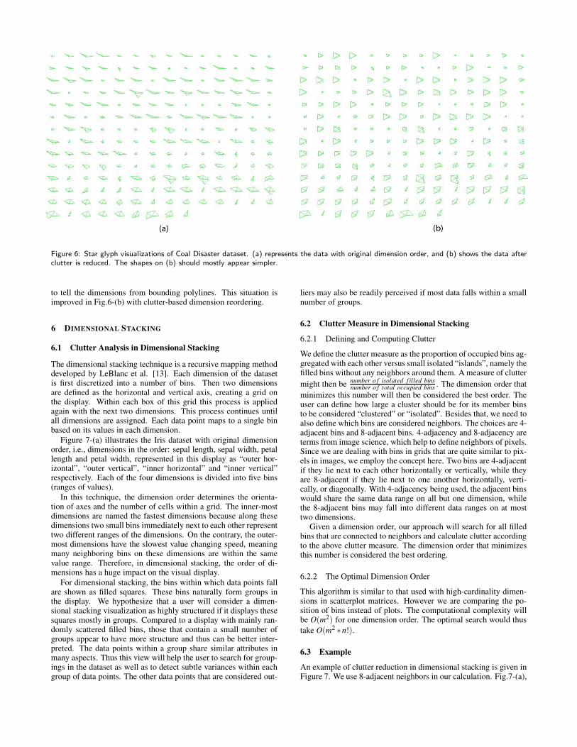
Figure 6: Star glyph visualizations of Coal Disaster dataset. (a) represents the data with original dimension order, and (b) shows the data afterclutter is reduced. The shapes on (b) should mostly appear simpler.

to tell the dimensions from bounding polylines. This situation isimproved in Fig.6-(b) with clutter-based dimension reordering.

6 DIMENSIONAL STACKING

6.1 Clutter Analysis in Dimensional Stacking

The dimensional stacking technique is a recursive mapping methoddeveloped by LeBlanc et al. [13]. Each dimension of the datasetis first discretized into a number of bins. Then two dimensionsare defined as the horizontal and vertical axis, creating a grid onthe display. Within each box of this grid this process is appliedagain with the next two dimensions. This process continues untilall dimensions are assigned. Each data point maps to a single binbased on its values in each dimension.

Figure 7-(a) illustrates the Iris dataset with original dimensionorder, i.e., dimensions in the order: sepal length, sepal width, petallength and petal width, represented in this display as “outer hor-izontal”, “outer vertical”, “inner horizontal” and “inner vertical”respectively. Each of the four dimensions is divided into five bins(ranges of values).

In this technique, the dimension order determines the orienta-tion of axes and the number of cells within a grid. The inner-mostdimensions are named the fastest dimensions because along thesedimensions two small bins immediately next to each other representtwo different ranges of the dimensions. On the contrary, the outer-most dimensions have the slowest value changing speed, meaningmany neighboring bins on these dimensions are within the samevalue range. Therefore, in dimensional stacking, the order of di-mensions has a huge impact on the visual display.

For dimensional stacking, the bins within which data points fallare shown as filled squares. These bins naturally form groups inthe display. We hypothesize that a user will consider a dimen-sional stacking visualization as highly structured if it displays thesesquares mostly in groups. Compared to a display with mainly ran-domly scattered filled bins, those that contain a small number ofgroups appear to have more structure and thus can be better inter-preted. The data points within a group share similar attributes inmany aspects. Thus this view will help the user to search for group-ings in the dataset as well as to detect subtle variances within eachgroup of data points. The other data points that are considered out-

liers may also be readily perceived if most data falls within a smallnumber of groups.

6.2 Clutter Measure in Dimensional Stacking

6.2.1 Defining and Computing Clutter

We define the clutter measure as the proportion of occupied bins ag-gregated with each other versus small isolated “islands”, namely thefilled bins without any neighbors around them. A measure of clutter

might then benumber o f isolated f illed binsnumber o f total occupied bins

. The dimension order that

minimizes this number will then be considered the best order. Theuser can define how large a cluster should be for its member binsto be considered “clustered” or “isolated”. Besides that, we need toalso define which bins are considered neighbors. The choices are 4-adjacent bins and 8-adjacent bins. 4-adjacency and 8-adjacency areterms from image science, which help to define neighbors of pixels.Since we are dealing with bins in grids that are quite similar to pix-els in images, we employ the concept here. Two bins are 4-adjacentif they lie next to each other horizontally or vertically, while theyare 8-adjacent if they lie next to one another horizontally, verti-cally, or diagonally. With 4-adjacency being used, the adjacent binswould share the same data range on all but one dimension, whilethe 8-adjacent bins may fall into different data ranges on at mosttwo dimensions.

Given a dimension order, our approach will search for all filledbins that are connected to neighbors and calculate clutter accordingto the above clutter measure. The dimension order that minimizesthis number is considered the best ordering.

6.2.2 The Optimal Dimension Order

This algorithm is similar to that used with high-cardinality dimen-sions in scatterplot matrices. However we are comparing the po-sition of bins instead of plots. The computational complexity willbe O(m2) for one dimension order. The optimal search would thus

take O(m2 ∗n!).

6.3 Example

An example of clutter reduction in dimensional stacking is given inFigure 7. We use 8-adjacent neighbors in our calculation. Fig.7-(a),

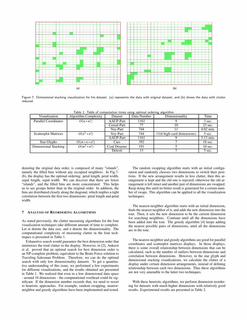
Figure 7: Dimensional stacking visualization for Iris dataset. (a) represents the data with original dataset, and (b) shows the data with clutterreduced.

Table 1: Table of computation times using optimal ordering algorithmVisualization Algorithm Complexity Dataset Data Number Dimensionality Time

Parallel Coordinates O(n∗n!) AAUP-Part 1161 9 3 sec.Cereal-Part 77 10 23 sec.

Voy-Part 744 11 4:02 min.

Scatterplot Matrices O(n2 ∗n!) Voy-Part 744 11(6 high-card dimensions) 5 sec.AAUP-Part 1161 9 3:13 min.

Star Glyphs O(m∗n∗n!) Cars 392 7 18 sec.

Dimensional Stacking O(m2 ∗n!) Coal Disaster 191 5 10 sec.Detroit 13 7 5 sec.

denoting the original data order, is composed of many “islands”,namely the filled bins without any occupied neighbors. In Fig.7-(b), the display has the optimal ordering: petal length, petal width,sepal length, sepal width. We can discover that there are fewer“islands”, and the filled bins are more concentrated. This helpsus to see groups better than in the original order. In addition, thebins are distributed closely along the diagonal, which implies a tightcorrelation between the first two dimensions: petal length and petalwidth.

7 ANALYSIS OF REORDERING ALGORITHMS

As stated previously, the clutter measuring algorithms for the fourvisualization techniques take different amount of time to complete.Let m denote the data size, and n denote the dimensionality. Thecomputational complexity of measuring clutter in the four tech-niques is presented in Table 1.

Exhaustive search would guarantee the best dimension order thatminimizes the total clutter in the display. However, in [2], Ankerstet al. proved that an optimal search for best dimension order isan NP-complete problem, equivalent to the Brute-Force solution toTraveling Salesman Problem. Therefore, we can do the optimalsearch with only low dimensionality datasets. To get a quantita-tive understanding of this issue, we performed a few experimentsfor different visualizations, and the results obtained are presentedin Table 1. We realized that even in a low dimensional data space- around 10 dimensions - the computational overhead could be sig-nificant. If the dimension number exceeds that, we need to resortto heuristic approaches. For example, random swapping, nearest-neighbor and greedy algorithms have been implemented and tested.

The random swapping algorithm starts with an initial configu-ration and randomly chooses two dimensions to switch their posi-tions. If the new arrangement results in less clutter, then this ar-rangement is kept and the old one is rejected; otherwise the old ar-rangement is left intact and another pair of dimensions are swapped.Keep doing this until no better result is generated for a certain num-ber of swaps. This algorithm can be applied to all the visualizationtechniques.

The nearest-neighbor algorithm starts with an initial dimension,finds the nearest neighbor of it, and adds the new dimension into thetour. Then, it sets the new dimension to be the current dimensionfor searching neighbors. Continue until all the dimensions havebeen added into the tour. The greedy algorithm [4] keeps addingthe nearest possible pairs of dimensions, until all the dimensionsare in the tour.

The nearest-neighbor and greedy algorithms are good for parallelcoordinates and scatterplot matrices displays. In those displays,there is some overall relationship between dimensions that can becalculated, such as the number of outliers between dimensions andcorrelation between dimensions. However, in the star glyph anddimensional stacking visualizations, we calculate the clutter of adisplay under certain dimension arrangements, instead of definingrelationship between each two dimensions. Thus these algorithmsare not very amenable to the latter two techniques.

With these heuristic algorithms, we perform dimension reorder-ing for datasets with much higher dimensions with relatively goodresults. Experimental results are presented in Table 2.

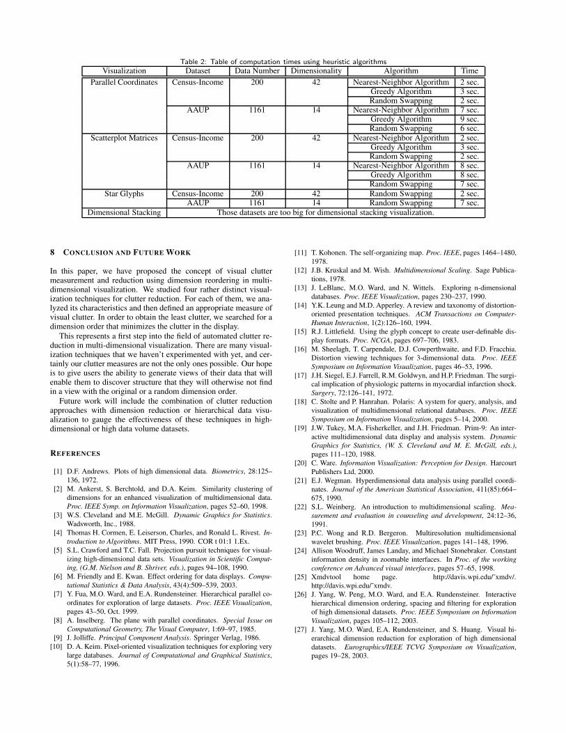
Table 2: Table of computation times using heuristic algorithmsVisualization Dataset Data Number Dimensionality Algorithm Time

Parallel Coordinates Census-Income 200 42 Nearest-Neighbor Algorithm 2 sec.Greedy Algorithm 3 sec.Random Swapping 2 sec.

AAUP 1161 14 Nearest-Neighbor Algorithm 7 sec.Greedy Algorithm 9 sec.Random Swapping 6 sec.

Scatterplot Matrices Census-Income 200 42 Nearest-Neighbor Algorithm 2 sec.Greedy Algorithm 3 sec.Random Swapping 2 sec.

AAUP 1161 14 Nearest-Neighbor Algorithm 8 sec.Greedy Algorithm 8 sec.Random Swapping 7 sec.

Star Glyphs Census-Income 200 42 Random Swapping 2 sec.AAUP 1161 14 Random Swapping 7 sec.

Dimensional Stacking Those datasets are too big for dimensional stacking visualization.

8 CONCLUSION AND FUTURE WORK

In this paper, we have proposed the concept of visual cluttermeasurement and reduction using dimension reordering in multi-dimensional visualization. We studied four rather distinct visual-ization techniques for clutter reduction. For each of them, we ana-lyzed its characteristics and then defined an appropriate measure ofvisual clutter. In order to obtain the least clutter, we searched for adimension order that minimizes the clutter in the display.

This represents a first step into the field of automated clutter re-duction in multi-dimensional visualization. There are many visual-ization techniques that we haven’t experimented with yet, and cer-tainly our clutter measures are not the only ones possible. Our hopeis to give users the ability to generate views of their data that willenable them to discover structure that they will otherwise not findin a view with the original or a random dimension order.

Future work will include the combination of clutter reductionapproaches with dimension reduction or hierarchical data visu-alization to gauge the effectiveness of these techniques in high-dimensional or high data volume datasets.

REFERENCES

[1] D.F. Andrews. Plots of high dimensional data. Biometrics, 28:125–

136, 1972.

[2] M. Ankerst, S. Berchtold, and D.A. Keim. Similarity clustering of

dimensions for an enhanced visualization of multidimensional data.

Proc. IEEE Symp. on Information Visualization, pages 52–60, 1998.

[3] W.S. Cleveland and M.E. McGill. Dynamic Graphics for Statistics.

Wadsworth, Inc., 1988.

[4] Thomas H. Cormen, E. Leiserson, Charles, and Ronald L. Rivest. In-

troduction to Algorithms. MIT Press, 1990. COR t 01:1 1.Ex.

[5] S.L. Crawford and T.C. Fall. Projection pursuit techniques for visual-

izing high-dimensional data sets. Visualization in Scientific Comput-

ing, (G.M. Nielson and B. Shriver, eds.), pages 94–108, 1990.

[6] M. Friendly and E. Kwan. Effect ordering for data displays. Compu-

tational Statistics & Data Analysis, 43(4):509–539, 2003.

[7] Y. Fua, M.O. Ward, and E.A. Rundensteiner. Hierarchical parallel co-

ordinates for exploration of large datasets. Proc. IEEE Visualization,

pages 43–50, Oct. 1999.

[8] A. Inselberg. The plane with parallel coordinates. Special Issue on

Computational Geometry, The Visual Computer, 1:69–97, 1985.

[9] J. Jolliffe. Principal Component Analysis. Springer Verlag, 1986.

[10] D. A. Keim. Pixel-oriented visualization techniques for exploring very

large databases. Journal of Computational and Graphical Statistics,

5(1):58–77, 1996.

[11] T. Kohonen. The self-organizing map. Proc. IEEE, pages 1464–1480,

1978.

[12] J.B. Kruskal and M. Wish. Multidimensional Scaling. Sage Publica-

tions, 1978.

[13] J. LeBlanc, M.O. Ward, and N. Wittels. Exploring n-dimensional

databases. Proc. IEEE Visualization, pages 230–237, 1990.

[14] Y.K. Leung and M.D. Apperley. A review and taxonomy of distortion-

oriented presentation techniques. ACM Transactions on Computer-

Human Interaction, 1(2):126–160, 1994.

[15] R.J. Littlefield. Using the glyph concept to create user-definable dis-

play formats. Proc. NCGA, pages 697–706, 1983.

[16] M. Sheelagh, T. Carpendale, D.J. Cowperthwaite, and F.D. Fracchia.

Distortion viewing techniques for 3-dimensional data. Proc. IEEE

Symposium on Information Visualization, pages 46–53, 1996.

[17] J.H. Siegel, E.J. Farrell, R.M. Goldwyn, and H.P. Friedman. The surgi-

cal implication of physiologic patterns in myocardial infarction shock.

Surgery, 72:126–141, 1972.

[18] C. Stolte and P. Hanrahan. Polaris: A system for query, analysis, and

visualization of multidimensional relational databases. Proc. IEEE

Symposium on Information Visualization, pages 5–14, 2000.

[19] J.W. Tukey, M.A. Fisherkeller, and J.H. Friedman. Prim-9: An inter-

active multidimensional data display and analysis system. Dynamic

Graphics for Statistics, (W. S. Cleveland and M. E. McGill, eds.),

pages 111–120, 1988.

[20] C. Ware. Information Visualization: Perception for Design. Harcourt

Publishers Ltd, 2000.

[21] E.J. Wegman. Hyperdimensional data analysis using parallel coordi-

nates. Journal of the American Statistical Association, 411(85):664–

675, 1990.

[22] S.L. Weinberg. An introduction to multidimensional scaling. Mea-

surement and evaluation in counseling and development, 24:12–36,

1991.

[23] P.C. Wong and R.D. Bergeron. Multiresolution multidimensional

wavelet brushing. Proc. IEEE Visualization, pages 141–148, 1996.

[24] Allison Woodruff, James Landay, and Michael Stonebraker. Constant

information density in zoomable interfaces. In Proc. of the working

conference on Advanced visual interfaces, pages 57–65, 1998.

[25] Xmdvtool home page. http://davis.wpi.edu/˜xmdv/.

http://davis.wpi.edu/˜xmdv.

[26] J. Yang, W. Peng, M.O. Ward, and E.A. Rundensteiner. Interactive

hierarchical dimension ordering, spacing and filtering for exploration

of high dimensional datasets. Proc. IEEE Symposium on Information

Visualization, pages 105–112, 2003.

[27] J. Yang, M.O. Ward, E.A. Rundensteiner, and S. Huang. Visual hi-

erarchical dimension reduction for exploration of high dimensional

datasets. Eurographics/IEEE TCVG Symposium on Visualization,

pages 19–28, 2003.