Scalable Quantum Simulation of Molecular Energies

P. J. J. O’Malley,1, ∗ R. Babbush,2, ∗ I. D. Kivlichan,3 J. Romero,3 J. R. McClean,4 R. Barends,5 J. Kelly,5 P.

Roushan,5 A. Tranter,6, 7 N. Ding,2 B. Campbell,1 Y. Chen,5 Z. Chen,1 B. Chiaro,1 A. Dunsworth,1 A. G. Fowler,5

E. Jeffrey,5 E. Lucero,5 A. Megrant,5 J. Y. Mutus,5 M. Neeley,5 C. Neill,1 C. Quintana,1 D. Sank,5 A. Vainsencher,1

J. Wenner,1 T. C. White,5 P. V. Coveney,7 P. J. Love,6 H. Neven,2 A. Aspuru-Guzik,3 and J. M. Martinis5, 1

1Department of Physics, University of California, Santa Barbara, CA 93106, USA2Google Inc., Venice, CA 90291, USA

3Department of Chemistry, Harvard University, Cambridge, MA 02138, USA4Computational Research Division, Lawrence Berkeley National Laboratory, Berkeley CA 94720, USA

5Google Inc., Santa Barbara, CA 93117, USA6Department of Physics, Tufts University, Medford, MA 02155, USA

7Center for Computational Science and Department of Chemistry, University College London, WC1H 0AJ, UK

We report the first electronic structure calculation performed on a quantum computer withoutexponentially costly precompilation. We use a programmable array of superconducting qubits tocompute the energy surface of molecular hydrogen using two distinct quantum algorithms. First,we experimentally execute the unitary coupled cluster method using the variational quantum eigen-solver. Our efficient implementation predicts the correct dissociation energy to within chemicalaccuracy of the numerically exact result. Second, we experimentally demonstrate the canonicalquantum algorithm for chemistry, which consists of Trotterization and quantum phase estimation.We compare the experimental performance of these approaches to show clear evidence that thevariational quantum eigensolver is robust to certain errors. This error tolerance inspires hope thatvariational quantum simulations of classically intractable molecules may be viable in the near future.

Universal and efficient simulation of physical systems[1] is among the most compelling applications of quan-tum computing. In particular, quantum simulation ofmolecular energies [2], which enables numerically exactprediction of chemical reaction rates, promises significantadvances in our understanding of chemistry and couldenable in silico design of new catalysts, pharmaceuti-cals and materials. As scalable quantum hardware be-comes increasingly viable [3–7], chemistry simulation hasattracted significant attention [8–28] since classically in-tractable molecules require a relatively modest numberof qubits and because solutions have commercial valueassociated with their chemical applications [29].

The fundamental challenge in building a quantum com-puter is realizing high-fidelity operations in a scalable ar-chitecture [30]. Superconducting qubits have made rapidprogress in recent years [3–6] and can be fabricated inmicrochip foundries and manufactured at scale [31]. Re-cent experiments have shown logic gate fidelities at thethreshold required for quantum error correction [3] anddynamical suppression of bit-flip errors [4]. Here, we usethe device reported in [4, 7, 32] to implement and com-pare two quantum algorithms for chemistry. We havepreviously characterized our hardware using randomizedbenchmarking [4] but related metrics (e.g. fidelities) onlyloosely bound how well our devices can simulate molecu-lar energies. Thus, studying the performance of hardwareon small instances of real problems is an important wayto measure progress towards viable quantum computing.

∗ These authors contributed equally to this work.

Our first experiment demonstrates the recently-proposed variational quantum eigensolver (VQE), intro-duced in [19]. Our VQE experiment achieves chemi-cal accuracy and is the first scalable quantum simula-tion of molecular energies performed on quantum hard-ware, in the sense that our algorithm is efficient anddoes not benefit from exponentially costly precompilation[33]. When implemented using a unitary coupled clusteransatz, VQE cannot be efficiently simulated classicallyand empirical evidence suggests that answers are accu-rate enough to predict chemical rates [19–23]. BecauseVQE only requires short state preparation and measure-ment sequences, it has been suggested that classicallyintractable computations might be possible using VQEwithout the overhead of error correction [22, 23]. Ourexperiments substantiate this notion; the robustness ofthe VQE to systematic device errors allows the experi-ment to achieve chemical accuracy.

Our second experiment realizes the original algorithmfor the quantum simulation of chemistry, introduced in[2]. This approach involves Trotterized simulation [34]and the quantum phase estimation algorithm (PEA) [35].We experimentally perform this entire algorithm, includ-ing both key components, for the first time. While PEAhas asymptotically better scaling in terms of precisionthan VQE, long and coherent gate sequences are requiredfor its accurate implementation.

The phase estimation component of the canonicalquantum chemistry algorithm has been demonstrated ina photonic system [36], a nuclear magnetic resonancesystem [37], and a nitrogen-vacancy center system [38].While all three experiments obtained molecular energiesto incredibly high precision, none of the experiments im-

arX

iv:1

512.

0686

0v2

[qu

ant-

ph]

4 F

eb 2

017

2

Time (ns)

PrepareInitial State

Apply Parameterized AnsatzMeasure

Expectation Values

Classical Optimizer Suggests New Parameters

CalculateEnergy

400 μm

Software

Hardware

0 100 200 300 400

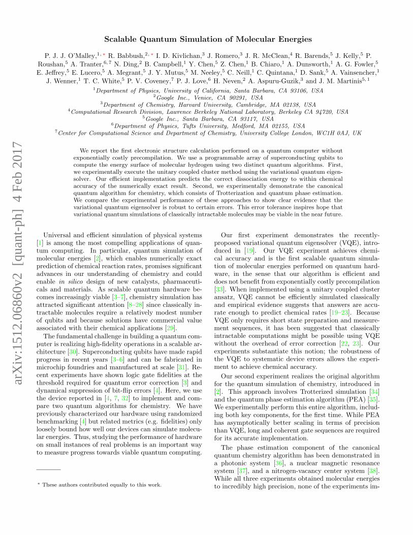
FIG. 1. Hardware and software schematic of the variational quantum eigensolver. (Hardware) micrograph showstwo Xmon transmon qubits and microwave pulse sequences to perform single-qubit rotations (thick lines), DC pulses fortwo-qubit entangling gates (dashed lines), and microwave spectrosopy tones for qubit measurements (thin lines). (Software)quantum circuit diagram shows preparation of Hartree-Fock state, followed by application of the unitary coupled cluster ansatzin Eq. (3) and efficient partial tomography (Rt) to measure the expectation values in Eq. (1). Finally, the total energy iscomputed according to Eq. (4) and provided to a classical optimizer which suggests new parameters.

plemented the propagator in a scalable fashion (e.g. usingTrotterization) as doing so requires long coherent evo-lutions. Furthermore, none of these experiments usedmore than a single qubit or qutrit to represent the en-tire molecule. This was possible due to the use of theconfiguration basis, which is not scalable but renders theexperimental challenge much easier. Furthermore, all ofthese implementations applied the logic gates with a sin-gle, totally controlled pulse, as opposed to compiling thealgorithm to a universal set of gates as we do.

There have been two previous experimental demon-strations of VQE: first in a photonic system [19] and laterin an ion trap [39]. Both experiments validated the vari-ational approach and the latter implemented an ansatzbased on unitary coupled cluster. All prior experimentsfocused on either molecular hydrogen [36, 37] or heliumhydride [19, 38, 39] but none of these prior experimentsemployed a scalable qubit representation such as secondquantization. Instead, all five prior experiments repre-sent the Hamiltonian in a configuration basis that cannotbe efficiently decomposed as a sum of local Hamiltonians,and then exponentiate this exponentially large matrix asa classical preprocessing step [19, 36–39].

Until this work, important aspects of scalable chem-istry simulation such as the Jordan-Wigner transforma-tion [40] or the Bravyi-Kitaev transformation [41, 42] hadnever been used to represent a molecule in an experi-ment; however, prior experiments such as [7] have pre-viously used the Jordan-Wigner representation to simu-late fermions on a lattice. In both experiments presentedhere, we simulate the dissociation of molecular hydro-gen in the minimal basis of Hartree-Fock orbitals, rep-resented using the Bravyi-Kitaev transformation of the

second quantized molecular Hamiltonian [17]. As shownin Appendix A, the molecular hydrogen Hamiltonian canbe scalably written as

H = g01+g1Z0 +g2Z1 +g3Z0Z1 +g4Y0Y1 +g5X0X1 (1)

where {Xi, Zi, Yi} denote Pauli matrices acting on the ith

qubit and the real scalars {gγ} are efficiently computablefunctions of the hydrogen-hydrogen bond length, R.

The ground state energy of Eq. (1) as a function ofR defines an energy surface. Such energy surfaces areused to compute chemical reaction rates which are expo-nentially sensitive to changes in energy. If accurate en-ergy surfaces are obtained, one can use established meth-ods such as classical Monte Carlo or Molecular Dynamicssimulations to obtain accurate free energies, which pro-vide the rates directly via the Erying equation [43]. Atroom temperature, a relative error in energy of 1.6×10−3

Hartree (1 kcal/mol or 0.043 eV) translates to a chemicalrate that differs from the true value by an order of magni-tude; therefore, 1.6×10−3 Hartree is known as “chemicalaccuracy” [43]. Our goal then is to compute the lowestenergy eigenvalues of Eq. (1) as a function of R, to withinchemical accuracy.

I. VARIATIONAL QUANTUM EIGENSOLVER

Many popular classical approximation methods for theelectronic structure problem involve optimizing a param-eterized guess wavefunction (known as an “ansatz”) ac-cording to the variational principle [43]. If we parameter-

ize an ansatz |ϕ(~θ)〉 by the vector ~θ then the variational

3

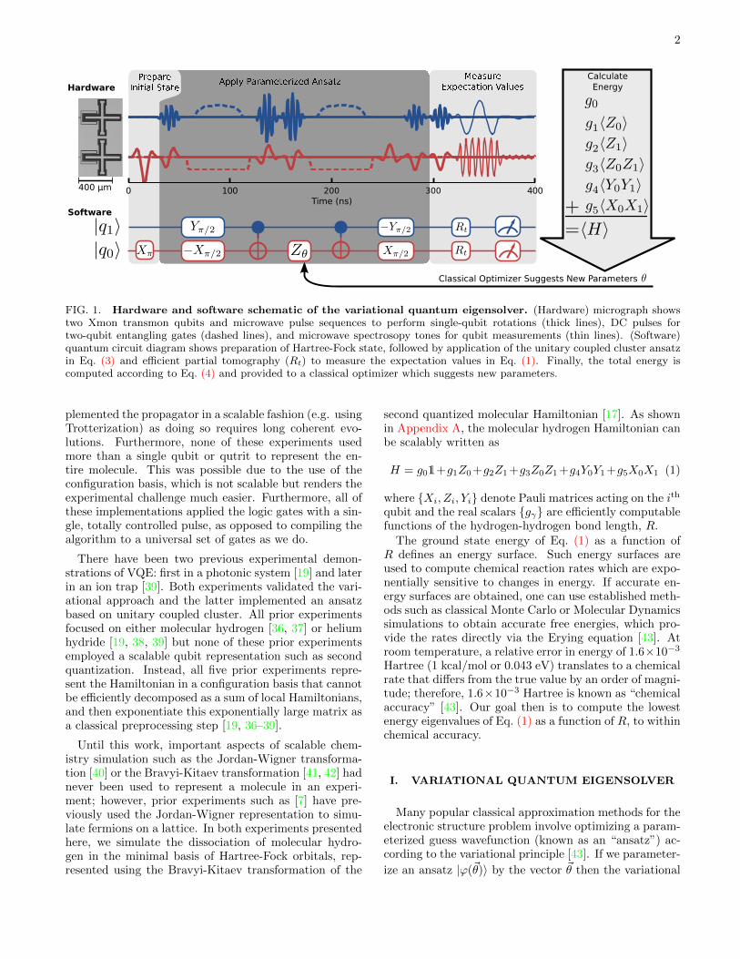
FIG. 2. Variational quantum eigensolver: raw data and computed energy surface. (a) Data showing the expectationvalues of terms in Eq. (1) as a function of θ, as in Eq. (3). Black lines nearest to the data show the theoretical values. Whilesuch systematic phase errors would prove disastrous for PEA, our VQE experiment is robust to this effect. (b) Experimentallymeasured energies (in Hartree) as a function of θ and R. This surface is computed from Figure 2a according to Eq. (4). Thewhite curve traces the theoretical minimum energy; the values of theoretical and experimental minima at each R are plottedin Figure 3a. Errors in this surface are given in Figure 6.

principle holds that

〈ϕ(~θ)|H |ϕ(~θ)〉〈ϕ(~θ)|ϕ(~θ)〉

≥ E0, (2)

where E0 is the smallest eigenvalue of the HamiltonianH. Accordingly, E0 can be estimated by selecting the pa-

rameters ~θ which minimize the left-hand side of Eq. (2).While the ground state wavefunction is likely to be in

superposition over an exponential number of states in thebasis of molecular orbitals, most classical approaches re-strict the ansatz to the support of polynomially manybasis elements due to memory limitations. However,quantum circuits can prepare entangled states which arenot known to be efficiently representable classically. In

VQE, the state |ϕ(~θ)〉 is parameterized by the action

of a quantum circuit U(~θ) on an initial state |φ〉, i.e.

|ϕ(~θ)〉 ≡ U(~θ) |φ〉. Even if |φ〉 is a simple product state

and U(~θ) is a very shallow circuit, |ϕ(~θ)〉 can containcomplex many-body correlations and span an exponen-tial number of standard basis states.

We can express the mapping U(~θ) as a concatenation ofparameterized quantum gates, U1(θ1)U2(θ2) · · ·Un(θn).In this work, we parameterize our circuit according tounitary coupled cluster theory [20, 22, 23]. As describedin Appendix D, unitary coupled cluster predicts that theground state of Eq. (1) can be expressed as

|ϕ(θ)〉 = e−i θ X0Y1 |01〉 , (3)

where |φ〉 = |01〉 is the Hartree-Fock (mean-field) stateof molecular hydrogen in the representation of Eq. (1).As discussed in Appendix D, unitary coupled cluster is

widely believed to be classically intractable and is knownto be strictly more powerful than the “gold standard” ofclassical electronic structure theory, coupled cluster [43–46]. The gate model circuit that performs this unitarymapping is shown in the software section of Figure 1.

VQE solves for the parameter vector ~θ with a clas-sical optimization routine. First, one prepares an ini-

tial ansatz |ϕ(~θ0)〉 and then estimates the ansatz energy

E(~θ0) by measuring the expectation values of each termin Eq. (1) and summing these values together as

E(~θ) =∑γ

gγ 〈ϕ(~θ)|Hγ |ϕ(~θ)〉 , (4)

where the gγ are scalars and the Hγ are local Hamilto-

nians as in Eq. (1). The initial guess ~θ0 and the corre-

sponding objective value E(~θ0) are then fed to a classi-cal greedy minimization routine (e.g. gradient descent),

which then suggests a new setting of the parameters ~θ1.

The energy E(~θ1) is then measured and returned to theclassical outer loop. This continues for m iterations until

the energy converges to a minimum value E(~θm) whichrepresents the VQE approximation to E0.

Because our experiment requires only a single varia-tional parameter, as in Eq. (3), we elected to scan a thou-sand different values of θ ∈ [−π, π) in order to obtain ex-pectation values which define the entire potential energycurve. We did this to simplify the classical feedback rou-tine but at the cost of needing slightly more experimentaltrials. These expectation values are shown in Figure 2aand the corresponding energy surfaces at different bondlengths are shown in Figure 2b. The energy surface in

4

0.5 1.0 1.5 2.0 2.5 3.0

Bond Length (Angstrom)

−1.2

−1.0

−0.8

−0.6

−0.4

−0.2

0.0

0.2TotalEnergy(Hartree)

Exact Energy

VQE Experiment

PEA Experiment

a b

0.5 1.0 1.5 2.0 2.5 3.0

Bond Length (Angstrom)

0.00

0.02

0.04

0.06

0.08

0.10

0.12

LocalError(Hartree)

equilibrium

Error at Experimental Angle

Error at Theoretical Angle

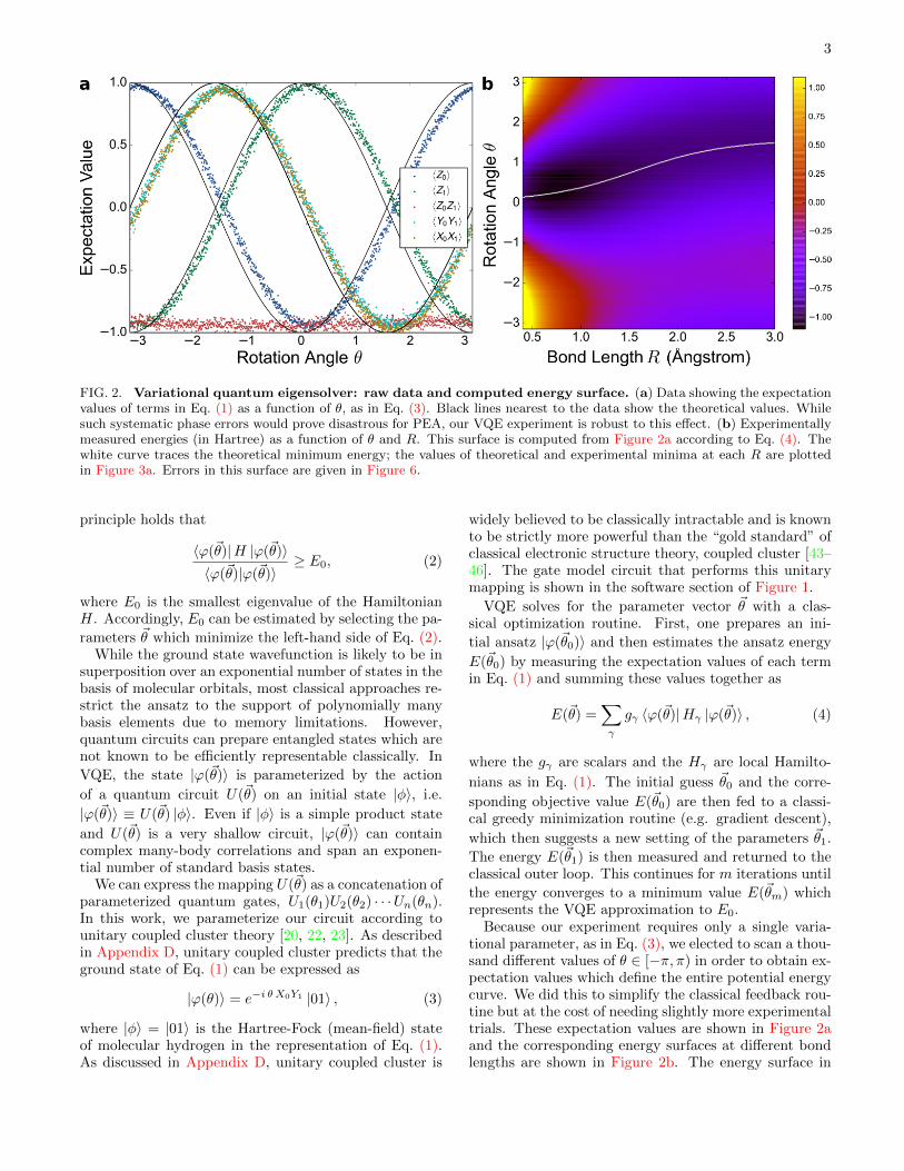
FIG. 3. Computed H2 energy curve and errors. (a) Energy surface of molecular hydrogen as determined by both VQEand PEA. VQE approach shows dissociation energy error of (8 ± 5) × 10−4 Hartree (error bars on VQE data are smaller thanmarkers). PEA approach shows dissociation energy error of (1 ± 1) × 10−2 Hartree. (b) Errors in VQE energy surface. Reddots show error in the experimentally determined energies. Green diamonds show the error in the energies that would havebeen obtained experimentally by running the circuit at the theoretically optimal θ instead of the experimentally optimal θ.The discrepancy between blue and red dots provides experimental evidence for the robustness of VQE which could not havebeen anticipated via numerical simulations. The gray band encloses the chemically accurate region relative to the experimentalenergy of the atomized molecule. The dissociation energy is relative to the equilibrium geometry, which falls within thisenvelope.

Figure 2b was locally optimized at each bond length toemulate an on-the-fly implementation.

Figure 3a shows the exact and experimentally deter-mined energies of molecular hydrogen at different bondlengths. The minimum energy bond length (R = 0.72 A)corresponds to the equilibrium bond length, whereas theasymptote on the right part of the curve corresponds todissociation into two hydrogen atoms. The energy differ-ence between these points is the dissociation energy, andthe exponential of this quantity determines the chem-ical dissociation rate. Our VQE experiment correctlypredicts this quantity with an error of (8 ± 5) × 10−4

Hartree, which is below the chemical accuracy threshold.Error bars are computed with Gaussian process regres-sion [47] which interpolates the energy surface based onlocal errors from the shot-noise limited expectation valuemeasurements in Figure 2a.

Errors in our simulation as a function of R are shownin Figure 3b. The curve in Figure 3b becomes nearly flatpast R = 2.5 A because the same angle is experimentallychosen for each R past this point. Note that the exper-imental energies are always greater than or equal to theexact energies due to the variational principle. Figure 3bshows that VQE has substantial robustness to system-atic errors. While this possibility had been previouslyhypothesized [23], we report the first experimental signa-ture of robustness and show that it allows for a successfulcomputation of the dissociation energy. By performing(inefficient) classical simulations of the circuit in Figure 1,we identify the theoretically optimal value of θ at each R.

In fact, for this system, at every value of R there existsθ such that E(θ) = E0. However, due to experimentalerror, the theoretically optimal value of θ differs substan-tially from the experimentally optimal value of θ. Thiscan be seen in Figure 3b from the large discrepancy be-tween the green diamonds (experimental energy errors attheoretically optimal θ) and the red dots (experimentalenergy errors at experimentally optimal θ). The experi-mental energy curve at theoretically optimal θ shows anerror in the dissociation energy of 1.1 × 10−2 Hartree,which is more than an order of magnitude worse. Onecould anticipate this discrepancy by looking at the rawdata in Figure 2a which shows that the experimentallymeasured expectation values deviate considerably fromthe predictions of theory. In a sense, the green diamondsin Figure 3b show the performance of a non-variationalalgorithm, which in theory gives the exact answer, butin practice fails due to systematic errors.

II. PHASE ESTIMATION ALGORITHM

We also report an experimental demonstration of theoriginal quantum algorithm for chemistry [2]. Similar toVQE, the first step of this algorithm is to prepare thesystem register in a state having good overlap with theground state of the Hamiltonian H. In our case, we beginwith the Hartree-Fock state, |φ〉. We then evolve thisstate under H using a Trotterized approximation to thetime-evolution operator. The execution of this unitary is

5

Time (μs)

PrepareInitial State

Evolve System,Acquire Phase on Ancilla

Convert Phase to Amplitude

400 μm

Hardware

Software

Measurebit

0.0 0.4 0.8 1.2 1.6

i

ii

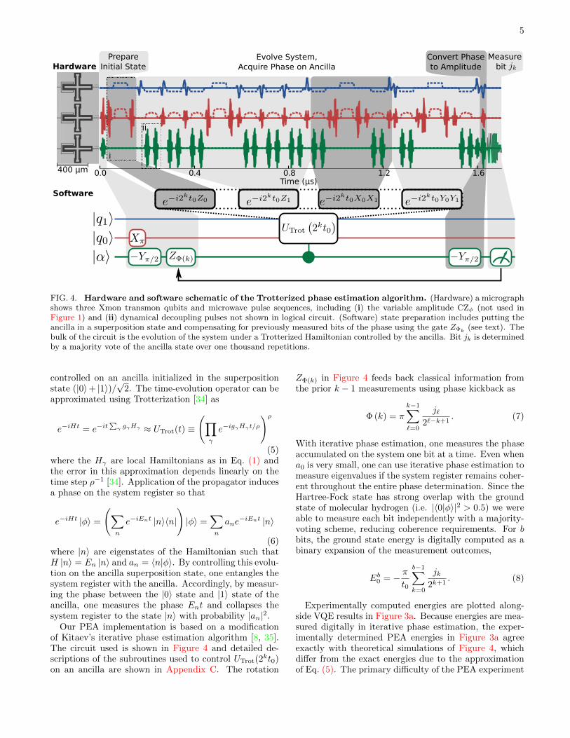
FIG. 4. Hardware and software schematic of the Trotterized phase estimation algorithm. (Hardware) a micrographshows three Xmon transmon qubits and microwave pulse sequences, including (i) the variable amplitude CZφ (not used inFigure 1) and (ii) dynamical decoupling pulses not shown in logical circuit. (Software) state preparation includes putting theancilla in a superposition state and compensating for previously measured bits of the phase using the gate ZΦk (see text). Thebulk of the circuit is the evolution of the system under a Trotterized Hamiltonian controlled by the ancilla. Bit jk is determinedby a majority vote of the ancilla state over one thousand repetitions.

controlled on an ancilla initialized in the superpositionstate (|0〉+ |1〉)/

√2. The time-evolution operator can be

approximated using Trotterization [34] as

e−iHt = e−it∑γ gγHγ ≈ UTrot(t) ≡

(∏γ

e−igγHγt/ρ

)ρ(5)

where the Hγ are local Hamiltonians as in Eq. (1) andthe error in this approximation depends linearly on thetime step ρ−1 [34]. Application of the propagator inducesa phase on the system register so that

e−iHt |φ〉 =

(∑n

e−iEnt |n〉〈n|)|φ〉 =

∑n

ane−iEnt |n〉

(6)where |n〉 are eigenstates of the Hamiltonian such thatH |n〉 = En |n〉 and an = 〈n|φ〉. By controlling this evolu-tion on the ancilla superposition state, one entangles thesystem register with the ancilla. Accordingly, by measur-ing the phase between the |0〉 state and |1〉 state of theancilla, one measures the phase Ent and collapses thesystem register to the state |n〉 with probability |an|2.

Our PEA implementation is based on a modificationof Kitaev’s iterative phase estimation algorithm [8, 35].The circuit used is shown in Figure 4 and detailed de-scriptions of the subroutines used to control UTrot(2

kt0)on an ancilla are shown in Appendix C. The rotation

ZΦ(k) in Figure 4 feeds back classical information fromthe prior k − 1 measurements using phase kickback as

Φ (k) = π

k−1∑`=0

j`2`−k+1

. (7)

With iterative phase estimation, one measures the phaseaccumulated on the system one bit at a time. Even whena0 is very small, one can use iterative phase estimation tomeasure eigenvalues if the system register remains coher-ent throughout the entire phase determination. Since theHartree-Fock state has strong overlap with the groundstate of molecular hydrogen (i.e. |〈0|φ〉|2 > 0.5) we wereable to measure each bit independently with a majority-voting scheme, reducing coherence requirements. For bbits, the ground state energy is digitally computed as abinary expansion of the measurement outcomes,

Eb0 = − πt0

b−1∑k=0

jk2k+1

. (8)

Experimentally computed energies are plotted along-side VQE results in Figure 3a. Because energies are mea-sured digitally in iterative phase estimation, the exper-imentally determined PEA energies in Figure 3a agreeexactly with theoretical simulations of Figure 4, whichdiffer from the exact energies due to the approximationof Eq. (5). The primary difficulty of the PEA experiment

6

is that the controlled application of UTrot(2kt0) requires

complex quantum circuitry and long coherent evolutions.Accordingly, we approximated the propagator in Eq. (5)using a single Trotter step (ρ = 1), which is not sufficientfor chemical accuracy. Our PEA experiment shows anerror in the dissociation energy of (1±1)×10−2 Hartree.

In addition to taking only one Trotter step, we per-formed classical simulations of the error in Eq. (5) underdifferent orderings of the Hγ in order to find the opti-mal Trotter sequences at each value of R. The Trottersequences used in our experiment as well as parameterssuch as t0 are reported in the Appendix C. Since thisoptimization is intractable for larger molecules, our PEAprotocol benefited from inefficient classical preprocessing(unlike our VQE implementation). Nevertheless, this isthe first time the canonical quantum algorithm for chem-istry has been executed in its entirety and as such, repre-sents a significant step towards scalable implementations.

III. EXPERIMENTAL METHODS

Both algorithms are implemented with a supercon-ducting quantum system based on the Xmon [48], a vari-ant of the planar transmon qubit [49], in a dilution re-frigerator with a base temperature of 20 mK. Each qubitconsists of a SQUID (superconducting quantum interfer-ence device), which provides a tunable nonlinear induc-tance, and a large X-shaped capacitor; qubit frequen-cies are tunable up to 6 GHz and have a nonlinearity of(ω21 − ω10) = −0.22 GHz. The qubits are capacitivelycoupled to their nearest neighbors in a linear chain pat-tern, with coupling strengths of 30 MHz. Single-qubitquantum gates are implemented with microwave pulsesand tuned using closed-loop optimization with random-ized benchmarking [50]. Qubit state measurement is per-formed in a dispersive readout scheme with capacitivelycoupled resonators at 6.6-6.8 GHz [4]. For details of thedevice fabrication and conventions for reporting qubitparameters, see [4].

Our entangling operation is a controlled-phase (CZφ)gate, accomplished by holding one of the qubits at a fixedfrequency while adiabatically tuning the other close to anavoided level crossing of the |11〉 and |02〉 states [3]. Toproduce the correct phase change φ, the acquired phaseis measured with quantum state tomography versus theamplitude of the trajectory, and the amplitude for anygiven φ is then determined via interpolation [7]. To min-imize leakage out of the computation subspace duringthis operation, we increase the gate duration from thepreviously used 40 ns to 50 ns, and then shape the pulsetrajectory. The CZφ gate as implemented here has arange of approximately 0.25 to 5.0 rad; for smaller val-ues of φ, parasitic interactions with other qubits becomenontrivial, and for larger φ, leakage is significant. Forφ outside this range, the total rotation is accomplishedwith two physical gates. For CZφ gates with φ = π, theamplitude and shape of the trajectory are further opti-

mized with ORBIT [50]. CZφ6=π is only necessary in thePEA experiment (see Appendix C).

The gates used to implement both VQE and PEA areshown in Appendix B and Appendix C. A single VQEsequence consists of 11 single-qubit gates and two CZπgates. A PEA sequence has at least 51 single-qubit gates,four CZφ6=π gates, and ten CZπ gates; more were requiredwhen not all φ values are within the range that could beperformed with a single physical gate.

IV. CONCLUSION

We report the use of quantum hardware to experimen-tally compute the potential energy curve of molecular hy-drogen using both PEA and VQE. We perform the firstexperimental implementation of the Trotterized molec-ular time-evolution operator and then measure energiesusing PEA. Due to the costly nature of Trotterization, weare able to implement only a single Trotter step, whichis not enough to achieve chemical accuracy. By con-trast, our VQE experiment achieves chemical accuracyand shows significant robustness to certain types of er-ror. The comparison of these two approaches suggeststhat adaptive algorithms (e.g. VQE) may generally bemore resilient for pre-error corrected quantum computingthan traditional gate model algorithms (e.g. PEA).

The robustness of VQE is partially a consequence ofthe adaptive nature of the algorithm; the classical outerloop of VQE helps to avoid systematic errors by actingsimilarly to the calibration loops used to tune individ-ual quantum gates [50]. This minimization proceduretreats the energy functional as a black box in that no as-sumptions are made about the actual circuit ansatz beingimplemented. Thus, VQE seeks to find the optimal pa-rameters in a fashion that is blind to control errors, suchas pulse imperfection, crosstalk and stray coupling in thedevice. We observe a remarkable increase in precisionby using the experimentally optimal parameters ratherthan the theoretically optimal parameters. This findinginspires hope that VQE may provide solutions to classi-cally intractable problems even without error correction.Additionally, these results motivate future experimentswhich take “sublogical” hardware calibration parameters,e.g. microwave pulse shapes, as variational parameters.

ACKNOWLEDGMENTS

The authors thank Cornelius Hempel for discussionsregarding VQE. J. R. M. is supported by the Luis W.Alvarez fellowship in Computing Sciences at LawrenceBerkeley National Laboratory. J. R. acknowledges theAir Force Office of Scientific Research for support un-der Award: FA9550-12-1-0046. A. A.-G. acknowledgesthe Army Research Office under Award: W911NF-15-1-0256 and the Defense Security Science Engineering Fel-lowship managed by the Office of Naval Research un-

7

der award N00014-16-1-2008. P. J. L. acknowledges thesupport of the National Science Foundation under grantnumber PHY-0955518. Devices were made at the UCSBNanofabrication Facility, a part of the NSF-funded Na-tional Nanotechnology Infrastructure Network, and atthe NanoStructures Cleanroom Facility. The authorsthank H. De Raedt, M. Nocon, D. Willsch and F. Jinwho brought to our attention an error in the g0 valuesreported in an earlier version of this work.

AUTHOR CONTRIBUTIONS

P. J. J. O. and R. Babbush contributed equally tothis work. R. Babbush, H.N., A.A.-G. and J.M.M. de-signed the experiments. P.J.J.O. performed the exper-

iments. J.K., R. Barends and A.M. fabricated the de-vice. I.D.K., J.R., J.R.M., A.T., N.D., P.V.C. and P.J.L.helped R. Babbush and P.J.J.O. to compile quantumsoftware and analyze data. R. Babbush, P.J.J.O., andJ.M.M. co-wrote the manuscript. All other authors con-tributed to the fabrication process, experimental set-upand manuscript preparation.

AUTHOR INFORMATION

Correspondence and requests for materials shouldbe addressed to P.J.J.O. (pomalley@google.com), R.Babbush (babbush@google.com), or J.M.M. (jmarti-nis@google.com).

[1] Seth Lloyd, “Universal Quantum Simulators,” Science273, 1073–1078 (1996).

[2] Alan Aspuru-Guzik, Anthony D Dutoi, Peter J Love,and Martin Head-Gordon, “Simulated Quantum Compu-tation of Molecular Energies,” Science 309, 1704 (2005).

[3] R Barends, J Kelly, A Megrant, A Veitia, D Sank,E Jeffrey, T C White, J Mutus, A G Fowler, Y Camp-bell Chen, Z Chen, B Chiaro, A Dunsworth, C Neill,P O’Malley, P Roushan, A Vainsencher, J Wenner, A NKorotkov, A N Cleland, and J Martinis, “Superconduct-ing quantum circuits at the surface code threshold forfault tolerance,” Nature 508, 500–503 (2014).

[4] J. Kelly, R. Barends, A. G. Fowler, A. Megrant, E. Jef-frey, T. C. White, D. Sank, J. Y. Mutus, B. Campbell,Yu Chen, Z. Chen, B. Chiaro, A. Dunsworth, I.-C. Hoi,C. Neill, P. J. J. O’Malley, C. Quintana, P. Roushan,A. Vainsencher, J. Wenner, A. N. Cleland, and John M.Martinis, “State preservation by repetitive error detec-tion in a superconducting quantum circuit,” Nature 519,66–69 (2015).

[5] A.D. Corcoles, Easwar Magesan, Srikanth J. Srinivasan,Andrew W. Cross, M. Steffen, Jay M. Gambetta, andJerry M. Chow, “Demonstration of a quantum error de-tection code using a square lattice of four superconduct-ing qubits,” Nature Communications 6, 6979 (2015).

[6] D Riste, S Poletto, M-Z Huang, A Bruno, V Vesterinen,O-P Saira, and L DiCarlo, “Detecting bit-flip errors ina logical qubit using stabilizer measurements.” NatureCommunications 6, 6983 (2015).

[7] R Barends, L Lamata, J Kelly, L Garcıa-Alvarez, A GFowler, A Megrant, E Jeffrey, T C White, D Sank,J Y Mutus, B Campbell, Yu Chen, Z Chen, B Chiaro,A Dunsworth, I-C Hoi, C Neill, P J J O’Malley, C Quin-tana, P Roushan, A Vainsencher, J Wenner, E Solano,and John M Martinis, “Digital quantum simulation offermionic models with a superconducting circuit,” Na-ture Communications 6, 7654 (2015).

[8] James D Whitfield, Jacob Biamonte, and Alan Aspuru-Guzik, “Simulation of electronic structure Hamiltoniansusing quantum computers,” Mol. Phys. 109, 735–750(2011).

[9] Ivan Kassal, James Whitfield, Alejandro Perdomo-Ortiz,Man-Hong Yung, and Alan Aspuru-Guzik, “SimulatingChemistry Using Quantum Computers,” Ann. Rev. Phys.Chem. 62, 185–207 (2010).

[10] N Cody Jones, James D Whitfield, Peter L McMa-hon, Man-Hong Yung, Rodney Van Meter, Alan Aspuru-Guzik, and Yoshihisa Yamamoto, “Faster quantumchemistry simulation on fault-tolerant quantum comput-ers,” New Journal of Physics 14, 115023 (2012).

[11] David Wecker, Bela Bauer, Bryan K. Clark, Matthew B.Hastings, and Matthias Troyer, “Gate-count estimatesfor performing quantum chemistry on small quantumcomputers,” Physical Review A 90, 1–13 (2014).

[12] David Poulin, M. B. Hastings, Dave Wecker, NathanWiebe, Andrew C. Doherty, and Matthias Troyer, “TheTrotter Step Size Required for Accurate Quantum Simu-lation of Quantum Chemistry,” Quantum Information &Computation 15, 361–384 (2015).

[13] Ryan Babbush, Jarrod McClean, Dave Wecker, AlanAspuru-Guzik, and Nathan Wiebe, “Chemical Basis ofTrotter-Suzuki Errors in Chemistry Simulation,” Physi-cal Review A 91, 022311 (2015).

[14] James D Whitfield, “Spin-free quantum computationalsimulations and symmetry adapted states,” Journal ofChemical Physics 139, 021105 (2013).

[15] Libor Veis and Jiı Pittner, “Adiabatic state preparationstudy of methylene,” The Journal of Chemical Physics140, 1–21 (2014).

[16] Libor Veis, Jakub Visak, Hiromi Nakai, and Jiı Pittner,“Quantum chemistry beyond Born-Oppenheimer approx-imation on a quantum computer: a simulated phase es-timation study,” e-print arXiv: 1507.03271 (2015).

[17] Andrew Tranter, Sarah Sofia, Jake Seeley, MichaelKaicher, Jarrod McClean, Ryan Babbush, Peter V.Coveney, Florian Mintert, Frank Wilhelm, and Pe-ter J. Love, “The Bravyi-Kitaev transformation: Proper-ties and applications,” International Journal of QuantumChemistry 115, 1431–1441 (2015).

[18] Ryan Babbush, Peter J. Love, and Alan Aspuru-Guzik,“Adiabatic Quantum Simulation of Quantum Chem-istry,” Scientific Reports 4, 1–11 (2014).

8

[19] Alberto Peruzzo, Jarrod McClean, Peter Shadbolt, Man-Hong Yung, Xiao-Qi Zhou, Peter J. Love, Alan Aspuru-Guzik, and Jeremy L. O’Brien, “A variational eigenvaluesolver on a photonic quantum processor,” Nature Com-munications 5, 1–7 (2014).

[20] Man-Hong Yung, J Casanova, A Mezzacapo, J. McClean,L Lamata, A. Aspuru-Guzik, and E Solano, “From tran-sistor to trapped-ion computers for quantum chemistry,”Scientific Reports 4, 9 (2014).

[21] Jarrod R. McClean, Ryan Babbush, Peter J. Love, andAlan Aspuru-Guzik, “Exploiting locality in quantumcomputation for quantum chemistry,” The Journal ofPhysical Chemistry Letters 5, 4368–4380 (2014).

[22] Dave Wecker, Matthew B. Hastings, and MatthiasTroyer, “Progress towards practical quantum variationalalgorithms,” Physical Review A 92, 042303 (2015).

[23] Jarrod R McClean, Jonathan Romero, Ryan Babbush,and Alan Aspuru-Guzik, “The theory of variationalhybrid quantum-classical algorithms,” New Journal ofPhysics 18, 23023 (2016).

[24] Borzu Toloui and Peter J. Love, “Quantum Algorithmsfor Quantum Chemistry based on the sparsity of the CI-matrix,” e-print arXiv: 1312.2579 (2013).

[25] Ryan Babbush, Dominic W. Berry, Ian D. Kivlichan,Annie Y. Wei, Peter J. Love, and Alan Aspuru-Guzik, “Exponentially More Precise Quantum Simula-tion of Fermions in Second Quantization,” New Journalof Physics 18, 033032 (2016).

[26] Ryan Babbush, Dominic W. Berry, Ian D. Kivlichan, An-nie Y. Wei, Peter J. Love, and Alan Aspuru-Guzik,“Exponentially More Precise Quantum Simulation ofFermions II: Quantum Chemistry in the CI Matrix Rep-resentation,” e-print arXiv: 1506.01029 (2015).

[27] Colin J. Trout and Kenneth R. Brown, “Magic state dis-tillation and gate compilation in quantum algorithms forquantum chemistry,” International Journal of QuantumChemistry 115, 1296–1304 (2015).

[28] Nikolaj Moll, Andreas Fuhrer, Peter Staar, and IvanoTavernelli, “Optimizing Qubit Resources for QuantumChemistry Simulations in Second Quantization on aQuantum Computer,” e-print arXiv:1510.04048 (2015).

[29] Leonie Mueck, “Quantum reform,” Nature Chemistry 7,361–363 (2015).

[30] John M Martinis, “Qubit metrology for building a fault-tolerant quantum computer,” e-print arXiv: 1502.01406(2015).

[31] M W Johnson, M H S Amin, S Gildert, T Lanting,F Hamze, N Dickson, R Harris, A J Berkley, J Johans-son, P Bunyk, E M Chapple, C Enderud, J P Hilton,K Karimi, E Ladizinsky, N Ladizinsky, T Oh, I Permi-nov, C Rich, M C Thom, E Tolkacheva, C J S Truncik,S Uchaikin, J Wang, B Wilson, and G Rose, “Quan-tum annealing with manufactured spins,” Nature 473,194–198 (2011).

[32] R. Barends, A. Shabani, L. Lamata, J. Kelly, A. Mezza-capo, U. Las Heras, R. Babbush, A. Fowler, B. Camp-bell, Y. Chen, Z. Chen, B. Chiaro, A. Dunsworth,E. Jeffrey, E. Lucero, A. Megrant, J. Mutus, M. Nee-ley, C. Neill, P. O’Malley, C. Quintana, P. Roushan,D. Sank, A. Vainsencher, J. Wenner, T. White, E. Solano,H. Neven, and J. Martinis, “Digitized Adiabatic Quan-tum Computing with a Superconducting Circuit,” Na-ture 534, 222–226 (2016).

[33] John A Smolin, Graeme Smith, and Alexander Vargo,“Oversimplifying quantum factoring.” Nature 499, 163–5 (2013).

[34] Hale F Trotter, “On the product of semi-groups of oper-ators,” Proc. Am. Math. Soc. 10, 545–551 (1959).

[35] Alexei Y. Kitaev, “Quantum measurements and theAbelian Stabilizer Problem,” e-print arXiv: 9511026(1995).

[36] B P Lanyon, J D Whitfield, G G Gillett, M E Goggin,M P Almeida, I Kassal, J D Biamonte, M Mohseni, B JPowell, M Barbieri, A Aspuru-Guzik, and a G White,“Towards quantum chemistry on a quantum computer.”Nature chemistry 2, 106–111 (2010).

[37] Jiangfeng Du, Nanyang Xu, Xinhua Peng, Pengfei Wang,Sanfeng Wu, and Dawei Lu, “NMR implementation of amolecular hydrogen quantum simulation with adiabaticstate preparation.” Physical Review Letters 104, 030502(2010).

[38] Ya Wang, Florian Dolde, Jacob Biamonte, Ryan Bab-bush, Ville Bergholm, Sen Yang, Ingmar Jakobi, PhilippNeumann, Alan Aspuru-Guzik, James D Whitfield, andJorg Wrachtrup, “Quantum Simulation of Helium Hy-dride Cation in a Solid-State Spin Register,” ACS Nano9, 7769–7774 (2015).

[39] Yangchao Shen, Xiang Zhang, Shuaining Zhang, Jing-Ning Zhang, Man-Hong Yung, and Kihwan Kim, “Quan-tum Implementation of Unitary Coupled Cluster for Sim-ulating Molecular Electronic Structure,” e-print arXiv:1506:00443 (2015).

[40] R. D. Somma, G. Ortiz, J.E. Gubernatis, E. Knill, andR. Laflamme, “Simulating physical phenomena by quan-tum networks,” Physical Review A 65, 17 (2002).

[41] Sergey Bravyi and Alexei Kitaev, “Fermionic quantumcomputation,” Annals of Physics 298, 210–226 (2002).

[42] Jacob T. Seeley, Martin J. Richard, and Peter J Love,“The Bravyi-Kitaev transformation for quantum com-putation of electronic structure,” Journal of ChemicalPhysics 137, 224109 (2012).

[43] T Helgaker, P Jorgensen, and J Olsen, Molecular Elec-tronic Structure Theory (Wiley, 2002).

[44] Mark R. Hoffmann and Jack Simons, “A unitary multi-configurational coupled-cluster method: Theory and ap-plications,” The Journal of Chemical Physics 88, 993(1988).

[45] Rodney J. Bartlett, Stanislaw A. Kucharski, and JozefNoga, “Alternative coupled-cluster ansatze II. The uni-tary coupled-cluster method,” Chemical Physics Letters155, 133–140 (1989).

[46] Andrew G. Taube and Rodney J. Bartlett, “New perspec-tives on unitary coupled-cluster theory,” InternationalJournal of Quantum Chemistry 106, 3393–3401 (2006).

[47] Christopher M Bishop, Pattern Recognition and MachineLearning (Springer, New York, 2006).

[48] R Barends, J Kelly, A Megrant, D Sank, E Jeffrey,Y Chen, Y Yin, B Chiaro, J Mutus, C Neill, P O’Malley,P Roushan, J Wenner, T C White, A N Cleland, andJohn M Martinis, “Coherent Josephson Qubit Suitablefor Scalable Quantum Integrated Circuits,” Physical Re-view Letters 111, 80502 (2013).

[49] Jens Koch, Terri Yu, Jay Gambetta, A Houck, D Schus-ter, J Majer, Alexandre Blais, M Devoret, S Girvin, andR Schoelkopf, “Charge-insensitive qubit design derivedfrom the Cooper pair box,” Physical Review A 76, 42319(2007).

9

[50] J Kelly, R Barends, B Campbell, Y Chen, Z Chen,B Chiaro, A. Dunsworth, a. G. Fowler, I.-C. Hoi, E Jef-frey, A. Megrant, J Mutus, C Neill, P J J O’Malley,C Quintana, P Roushan, D Sank, A. Vainsencher, J Wen-ner, T C White, A N Cleland, and John M Martinis,“Optimal Quantum Control Using Randomized Bench-marking,” Physical Review Letters 112, 240504 (2014).

Appendix A: The electronic structure problem

The central problem of quantum chemistry is to com-pute the lowest energy eigenvalue of the molecular elec-tronic structure Hamiltonian. The eigenstates of thisHamiltonian determine almost all of the properties of in-terest in a molecule or material, and as the gap betweenthe ground and first electronically excited state is oftenmuch larger than the thermal energy at room tempera-ture, the ground state is of particular interest. To arriveat the standard form of this Hamiltonian used in quan-tum computation, one begins from a collection of nuclearcharges Zi and a number of electrons in the system N forwhich the corresponding Hamiltonian is written

H = −∑i

∇2Ri

2Mi−∑i

∇2ri

2−∑i,j

Zi|Ri − rj |

+∑i,j>i

ZiZj|Ri −Rj |

+∑i,j>i

1

|ri − rj |(A1)

where the positions, masses, and charges of the nucleiare Ri,Mi, Zi, and the positions of the electrons are ri.Here, the Hamiltonian is in atomic units of energy known

as Hartree. One Hartree is ~2

mee2a20(630 kcal/mol or 27.2

eV) where me, e and a0 denote the mass of an electron,charge of an electron and Bohr radius, respectively.

This form of the Hamiltonian and its real-space dis-cretization are often referred to as the first quantizedformulation of quantum chemistry. Several approacheshave been developed for treating this form of the prob-lem on a quantum computer [9]; however, the focus of thiswork is the second quantized formulation. To reach thesecond quantized formulation, one typically first approx-imates the nuclei as fixed classical point charges underthe Born-Oppenhemier approximation, chooses a basisφi in which to represent the wavefunction, and enforcesanti-symmetry with the fermion creation and annihila-

tion operators a†i and aj to give

H =∑pq

hpqa†paq +

1

2

∑pqrs

hpqrsa†pa†qaras (A2)

with

hpq =

∫dσ φ∗p(σ)

(∇2r

2−∑i

Zi|Ri − r|

)φq(σ) (A3)

hpqrs =

∫dσ1 dσ2

φ∗p(σ1)φ∗q(σ2)φs(σ1)φr(σ2)

|r1 − r2|(A4)

where σi is now a spatial and spin coordinate with σi =(ri, si), and the standard anti-commutation relations

that determine the action of a†i and aj are {a†i , aj} = δijand {a†i , a†j} = {ai, aj} = 0. Finally, the second quan-tized Hamiltonian must be mapped into qubits for im-plementation on a quantum device. The most commonmappings used for this purpose are the Jordan-Wignertransformation [40] and the Bravyi-Kitaev transforma-tion [17, 41, 42].

Classical Preparation

Phase Estimation Algorithm Variational Quantum Eigensolver

Real SpaceMolecular

Hamiltonian

Entangle Ancillawith Trotterized

Propagator

ComputeNew Parameters

Compute Orbitals,Hartree-Fock State

ApplyParameterized

Unitary

Bravyi-KitaevTransform

Write inSecond Quantized

Orbital Basis

Born-OppenheimerApproximation

MeasureExpectation

Values

MeasureAncillaPhase

Repeat UntilGround State

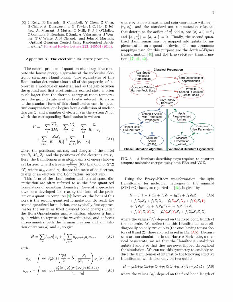
FIG. 5. A flowchart describing steps required to quantumcompute molecular energies using both PEA and VQE.

Using the Bravyi-Kitaev transformation, the spinHamiltonian for molecular hydrogen in the minimal(STO-6G) basis, as reported in [42], is given by

H = f01+ f1Z0 + f2Z1 + f3Z2 + f1Z0Z1 (A5)

+ f4Z0Z2 + f5Z1Z3 + f6X0Z1X2 + f6Y0Z1Y2

+ f7Z0Z1Z2 + f4Z0Z2Z3 + f3Z1Z2Z3

+ f6X0Z1X2Z3 + f6Y0Z1Y2Z3 + f7Z0Z1Z2Z3

where the values {fi} depend on the fixed bond length ofthe molecule. We notice that this Hamiltonian acts off-diagonally on only two qubits (the ones having tensor fac-tors of 0 and 2), those colored in red in Eq. (A5). Becausewe start our simulations in the Hartree-Fock state, a clas-sical basis state, we see that the Hamiltonian stabilizesqubits 1 and 3 so that they are never flipped throughoutthe simulation. We can use this symmetry to scalably re-duce the Hamiltonian of interest to the following effectiveHamiltonian which acts only on two qubits,

H = g01+g1Z0+g2Z1+g3Z0Z1+g4X0X1+g5Y0Y1 (A6)

where the values {gi} depend on the fixed bond length of

10

the molecule. We further note that the term Z0Z1 com-mutes with all other terms in the Hamiltonian. Sincethe ground state of the total Hamiltonian certainly hassupport on the Hartree-Fock state, we know the contri-bution to the total energy of Z0Z1 (it is given by theexpectation of those terms with the Hartree-Fock state).Steps to prepare this Hamiltonian are summarized in theupper-half of Figure 5.

Appendix B: Experimental methods for VQE

For the VQE experiment, the qubits q0 and q1 are used,at 4.49 and 5.53 GHz, respectively, while all the otherqubits are detuned to 3 GHz and below. Xπ, Yπ, ±Xπ/2,and ±Yπ/2 gates are 25 ns long, and pulse amplitudesand detunings from f10 are optimized with ORBIT; forthese parameters, additional pulse shaping (e.g. DRAG)proved unnecessary (see [32] for details of pulse detuningand shaping). The amplitude, trajectory, and compen-sating single-qubit phases of the CZπ gate are optimizedwith ORBIT as well. The duration of the CZπ is 55 ns,during which the frequency of q0 is fixed and q1 is moved.The rotation Zθ (the adjustable parameter in Eq. (3)) isimplemented as a phase shift on all subsequent gates.As operated here, q0 and q1 have energy relaxation timesT1 = 62.8 and 21.4µs, and Ramsey decay times T ∗2 = 1.1and 1.9µs, respectively.

The expectation values used to calculate the energy ofthe prepared state are measured with partial tomogra-phy; for example, X1X0 is measured by applying Yπ/2gates to each qubit prior to measurement. We empha-size that for chemistry problems, the number of measure-ments scales polynomially [23]. Readout duration is setto 1000 ns for higher fidelity (compared to [4], where the“measure”/odd-numbered qubits utilized much shorterreadout). In addition to discriminating between |0〉 and|1〉, higher level qubit states were also measured (called|2〉 for simplicity). Readout fidelities are typically >99%for |0〉, and ∼95% for |1〉 and |2〉, and measurement prob-abilities are corrected for readout error. After readoutcorrection, experiments where one of the qubits is mea-sured in |2〉 are dropped; any probability to be in |2〉 isset to zero and remaining probabilities are renormalized.

The circuit pulse sequence used to implement the UCCsequence in Eq. (3) is shown in Figure 1. The experimentis performed in different gauges of the Bravyi-Kitaevtransform; these correspond to the |0〉 (|1〉) state of q0

representing the first orbital being unoccupied (occupied)or occupied (unoccupied), and similarly for q1 represent-ing the parity of the first two orbitals being even (odd) orodd (even). In practice, a gauge change means a flip ofthe value of one or both qubits in the Hartree-Fock (HF)input state, and a sign change on the relevant terms ofthe Hamiltonian. In the standard gauge, the HF state is|01〉 and is prepared with an Xπ gate on q0. Statisticsfrom the experiment in these gauges are then averagedtogether. We also drop the first −Yπ/2 on q0; for an input

0.5 1.0 1.5 2.0 2.5 3.0

Bond Length R (Angstrom)

−3

−2

−1

0

1

2

3

Rot

atio

nA

ngle

Θ

−0.20

−0.16

−0.12

−0.08

−0.04

0.00

0.04

0.08

0.12

0.16

0.20

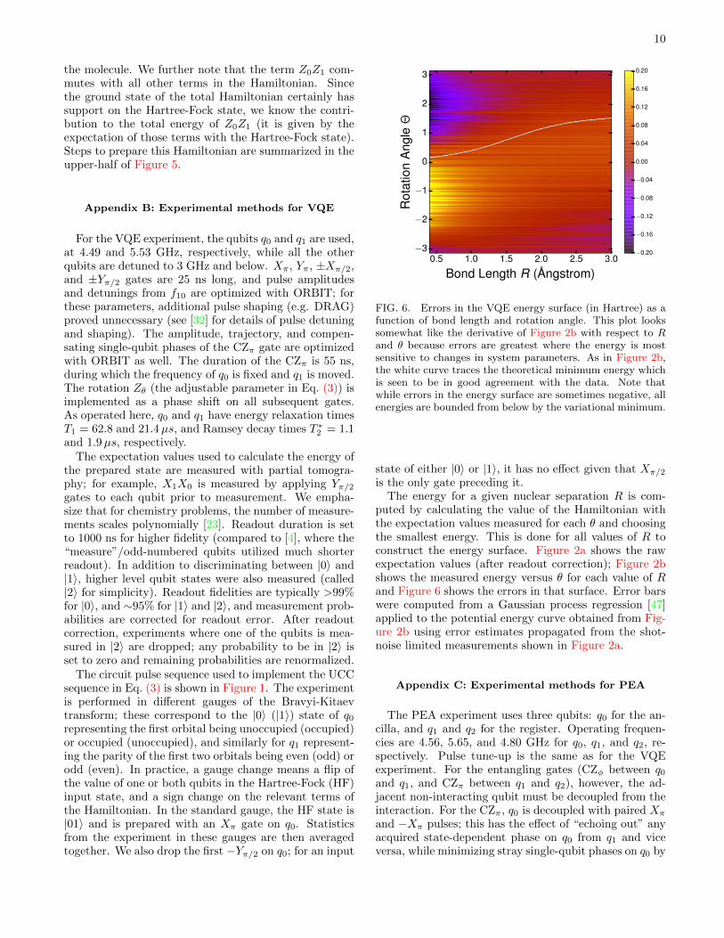
FIG. 6. Errors in the VQE energy surface (in Hartree) as afunction of bond length and rotation angle. This plot lookssomewhat like the derivative of Figure 2b with respect to Rand θ because errors are greatest where the energy is mostsensitive to changes in system parameters. As in Figure 2b,the white curve traces the theoretical minimum energy whichis seen to be in good agreement with the data. Note thatwhile errors in the energy surface are sometimes negative, allenergies are bounded from below by the variational minimum.

state of either |0〉 or |1〉, it has no effect given that Xπ/2

is the only gate preceding it.The energy for a given nuclear separation R is com-

puted by calculating the value of the Hamiltonian withthe expectation values measured for each θ and choosingthe smallest energy. This is done for all values of R toconstruct the energy surface. Figure 2a shows the rawexpectation values (after readout correction); Figure 2bshows the measured energy versus θ for each value of Rand Figure 6 shows the errors in that surface. Error barswere computed from a Gaussian process regression [47]applied to the potential energy curve obtained from Fig-ure 2b using error estimates propagated from the shot-noise limited measurements shown in Figure 2a.

Appendix C: Experimental methods for PEA

The PEA experiment uses three qubits: q0 for the an-cilla, and q1 and q2 for the register. Operating frequen-cies are 4.56, 5.65, and 4.80 GHz for q0, q1, and q2, re-spectively. Pulse tune-up is the same as for the VQEexperiment. For the entangling gates (CZφ between q0

and q1, and CZπ between q1 and q2), however, the ad-jacent non-interacting qubit must be decoupled from theinteraction. For the CZπ, q0 is decoupled with paired Xπ

and −Xπ pulses; this has the effect of “echoing out” anyacquired state-dependent phase on q0 from q1 and viceversa, while minimizing stray single-qubit phases on q0 by

11

keeping its frequency stationary. For the CZφ, however,q2 is detuned to frequencies significantly below the q0-q1

interaction; while this makes single-qubit phases on q2

harder to compensate, it is more effective at minimizingthe impact of q2 on the CZφ gate. This combination ofdecoupling methods was found to be optimal to minimizeerror on the phase of q0, which is the critical parameterin the PEA experiment.

As the CZφ gate varies the amplitude of q1’s frequencytrajectory over a wide range (approximately 200 MHzto 950 MHz) particular values of φ can be more sensitivelossy parts of the q1’s frequency spectrum that are rapidlyswept past and easily compensated for in the standardcase of only tuning up φ = π. Therefore, for some valuesof φ it is necessary to individually tune in compensatingphases on q0. This is implemented by executing the indi-vidual term of the Hamiltonian, varying the compensat-ing phase on q0, and fitting for the value that minimizesthe error of that term. After performing this careful com-pensation when necessary, the experiment produces thebit values (0 or 1) for each different Hamiltonian (i.e.each separation R) at each evolution time t that matchthose predicted by numerical simulation.

As operated in this experiment, q0, q1, and q2 have T1

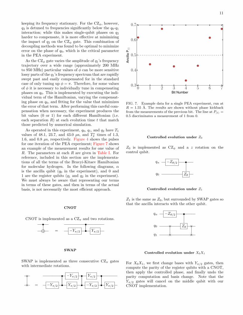
values of 48.1, 23.7, and 43.0 µs, and T ∗2 times of 1.3,1.6, and 0.8 µs, respectively. Figure 4 shows the pulsesfor one iteration of the PEA experiment; Figure 7 showsan example of the measurement results for one value ofR. The parameters at each R are given in Table I. Forreference, included in this section are the implementa-tions of all the terms of the Bravyi-Kitaev Hamiltonianfor molecular hydrogen. In the following diagrams, αis the ancilla qubit (q0 in the experiment), and 0 and1 are the register qubits (q1 and q2 in the experiment).We must always be aware that representing our termsin terms of these gates, and then in terms of the actualbasis, is not necessarily the most efficient approach.

CNOT

CNOT is implemented as a CZπ and two rotations.

• •= −Yπ/2 • Yπ/2

SWAP

SWAP is implemented as three consecutive CZπ gateswith intermediate rotations.

× • −Yπ/2 • Yπ/2 •

× = −Yπ/2 • Yπ/2 • −Yπ/2 • Yπ/2

0 1 2 3 4 5 6 7Bit Number

0.3

0.4

0.5

0.6

0.7

Anc

illa

P|1〉

FIG. 7. Example data for a single PEA experiment, run atR = 1.55 A. The results are shown without phase kickbackfrom the measurements of the previous bit. The line at P|1〉 =0.5 discriminates a measurement of 1 from 0.

Controlled evolution under Z0

Z0 is implemented as CZφ and a z rotation on thecontrol qubit.

qα −Zθ/2 •

q0 Zθ

Controlled evolution under Z1

Z1 is the same as Z0, but surrounded by SWAP gates sothat the ancilla interacts with the other qubit.

qα −Zθ/2 •

q0 × Zθ ×

q1 × ×

Controlled evolution under X0X1

For X0X1, we first change bases with Yπ/2 gates, thencompute the parity of the register qubits with a CNOT,then apply the controlled phase, and finally undo theparity computation and basis change. Note that theYπ/2 gates will cancel on the middle qubit with ourCNOT implementation.

12

qα −Zθ/2 •

q0 Yπ/2 Zθ −Yπ/2

q1 Yπ/2 • • −Yπ/2

Controlled evolution under Y0Y1

Y0Y1 is the same as X0X1 with a different basis change.

qα −Zθ/2 •

q0 −Xπ/2 Zθ Xπ/2

q1 −Xπ/2 • • Xπ/2

Appendix D: Unitary coupled cluster

The application of VQE requires the choice of anansatz, and in this work we have focused on the uni-tary coupled cluster (UCC) ansatz. This ansatz is a uni-tary variant of the method sometimes referred to as the“gold standard of quantum chemistry”, namely coupledcluster with single and double excitations with pertur-bative triples excitations [43]. The unitary variant hasthe advantage of satisfying a variational principle withrespect to all possible parameterizations [44–46]. Fur-thermore, UCC can be easily applied to a multireferenceinitial state whereas one of the major shortcomings oftraditional coupled cluster is that it can only be appliedto a single Slater determinant [44–46]. While the unitaryvariant has no efficient preparation scheme on a classi-cal computer, scalable methods of preparation for a fixedset of parameters on a quantum device have now beendocumented several times [19, 20, 22, 23].

The UCC ansatz |ϕ(~θ)〉 is defined with respect to areference state, which in this work we take to be theHartree-Fock state |φ〉,

|ϕ(~θ)〉 = U(~θ) |ϕ〉 = eT (~θ)−T (~θ)† |φ〉 (D1)

where T (~θ) is the anti-Hermitian cluster operator:

T =∑k

(k)T (~θ) (D2)

(1)T (~θ) =∑i1∈occa1∈virt

θa1i1 a†a1ai1 (D3)

(2)T (~θ) =1

4

∑i1,i2∈occa1,a2∈virt

θa1,a2i1,i2a†a2ai2a

†a1ai1 (D4)

where the occ and virt spaces are defined as the occu-pied and unoccupied sites in the Hartree-Fock state andthe definition of higher-order cluster operators (k)T fol-lows naturally. When only including up to the first twoterms in the cluster expansion, we term the ansatz uni-tary coupled cluster with single and doubles excitations(UCCSD) [43].

The task within VQE is to determine the optimal val-ues of the one- and two-body cluster amplitudes θa1i1 and

θa1,a2i1,i2, which are determined by the variational minimum

of a nonlinear function. As with all nonlinear minimiza-tions, the choice of starting parameters is key to algo-rithmic performance. As in classical coupled cluster,we can determine the starting amplitudes perturbativelythrough Moller-Plesset perturbation theory (MP2) [43].For molecular hydrogen in the minimal basis, there isexactly one term in the UCCSD ansatz.

The MP2 guess amplitudes are given by the equations

θai = 0, θabij =hijba − hijab

εi + εj − εa − εb(D5)

where εa refer to the 1-electron occupied and virtual or-bital energies from the Hartree-Fock calculation and thehijab are computed as in Eq. (A3). In the MP2 guess,the vanishing of the singles amplitudes is a result of thefact that single excitations away from the Hartree-Fockreference do not couple through the Hamiltonian as aconsequence of Brillouin’s theorem [43]. As the solu-tion of the classical coupled cluster equations is also effi-cient, it is possible to use amplitudes from a method likeCCSD as starting values as well. We note in both caseshowever, that the single-reference, perturbative nature ofthese constructions may lead to poor initial guesses forsystems with strong multireference character or entan-glement. In these cases the amplitudes may representpoor guesses, requiring more iterations for convergence.As such, a better initial guess in such problems may be arelated optimization, such as a different molecular geom-etry of the same system. In cases where the perturbativeestimates are accurate, one can discard operations re-lated to very small amplitudes in the state preparationcircuit, leading to computational savings.

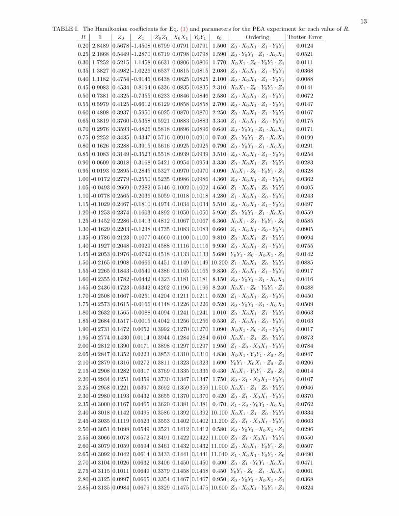
13TABLE I. The Hamiltonian coefficients for Eq. (1) and parameters for the PEA experiment for each value of R.

R 11 Z0 Z1 Z0Z1 X0X1 Y0Y1 t0 Ordering Trotter Error

0.20 2.8489 0.5678 -1.4508 0.6799 0.0791 0.0791 1.500 Z0 ·X0X1 · Z1 · Y0Y1 0.0124

0.25 2.1868 0.5449 -1.2870 0.6719 0.0798 0.0798 1.590 Z0 · Y0Y1 · Z1 ·X0X1 0.0521

0.30 1.7252 0.5215 -1.1458 0.6631 0.0806 0.0806 1.770 X0X1 · Z0 · Y0Y1 · Z1 0.0111

0.35 1.3827 0.4982 -1.0226 0.6537 0.0815 0.0815 2.080 Z0 ·X0X1 · Z1 · Y0Y1 0.0368

0.40 1.1182 0.4754 -0.9145 0.6438 0.0825 0.0825 2.100 Z0 ·X0X1 · Z1 · Y0Y1 0.0088

0.45 0.9083 0.4534 -0.8194 0.6336 0.0835 0.0835 2.310 X0X1 · Z0 · Y0Y1 · Z1 0.0141

0.50 0.7381 0.4325 -0.7355 0.6233 0.0846 0.0846 2.580 Z0 ·X0X1 · Z1 · Y0Y1 0.0672

0.55 0.5979 0.4125 -0.6612 0.6129 0.0858 0.0858 2.700 Z0 ·X0X1 · Z1 · Y0Y1 0.0147

0.60 0.4808 0.3937 -0.5950 0.6025 0.0870 0.0870 2.250 Z0 ·X0X1 · Z1 · Y0Y1 0.0167

0.65 0.3819 0.3760 -0.5358 0.5921 0.0883 0.0883 3.340 Z1 ·X0X1 · Z0 · Y0Y1 0.0175

0.70 0.2976 0.3593 -0.4826 0.5818 0.0896 0.0896 0.640 Z0 · Y0Y1 · Z1 ·X0X1 0.0171

0.75 0.2252 0.3435 -0.4347 0.5716 0.0910 0.0910 0.740 Z0 · Y0Y1 · Z1 ·X0X1 0.0199

0.80 0.1626 0.3288 -0.3915 0.5616 0.0925 0.0925 0.790 Z0 · Y0Y1 · Z1 ·X0X1 0.0291

0.85 0.1083 0.3149 -0.3523 0.5518 0.0939 0.0939 3.510 Z0 ·X0X1 · Z1 · Y0Y1 0.0254

0.90 0.0609 0.3018 -0.3168 0.5421 0.0954 0.0954 3.330 Z0 ·X0X1 · Z1 · Y0Y1 0.0283

0.95 0.0193 0.2895 -0.2845 0.5327 0.0970 0.0970 4.090 X0X1 · Z0 · Y0Y1 · Z1 0.0328

1.00 -0.0172 0.2779 -0.2550 0.5235 0.0986 0.0986 4.360 Z0 ·X0X1 · Z1 · Y0Y1 0.0362

1.05 -0.0493 0.2669 -0.2282 0.5146 0.1002 0.1002 4.650 Z1 ·X0X1 · Z0 · Y0Y1 0.0405

1.10 -0.0778 0.2565 -0.2036 0.5059 0.1018 0.1018 4.280 Z1 ·X0X1 · Z0 · Y0Y1 0.0243

1.15 -0.1029 0.2467 -0.1810 0.4974 0.1034 0.1034 5.510 Z0 ·X0X1 · Z1 · Y0Y1 0.0497

1.20 -0.1253 0.2374 -0.1603 0.4892 0.1050 0.1050 5.950 Z0 · Y0Y1 · Z1 ·X0X1 0.0559

1.25 -0.1452 0.2286 -0.1413 0.4812 0.1067 0.1067 6.360 X0X1 · Z1 · Y0Y1 · Z0 0.0585

1.30 -0.1629 0.2203 -0.1238 0.4735 0.1083 0.1083 0.660 Z1 ·X0X1 · Z0 · Y0Y1 0.0905

1.35 -0.1786 0.2123 -0.1077 0.4660 0.1100 0.1100 9.810 Z0 ·X0X1 · Z1 · Y0Y1 0.0694

1.40 -0.1927 0.2048 -0.0929 0.4588 0.1116 0.1116 9.930 Z0 ·X0X1 · Z1 · Y0Y1 0.0755

1.45 -0.2053 0.1976 -0.0792 0.4518 0.1133 0.1133 5.680 Y0Y1 · Z0 ·X0X1 · Z1 0.0142

1.50 -0.2165 0.1908 -0.0666 0.4451 0.1149 0.1149 10.200 Z1 ·X0X1 · Z0 · Y0Y1 0.0885

1.55 -0.2265 0.1843 -0.0549 0.4386 0.1165 0.1165 9.830 Z0 ·X0X1 · Z1 · Y0Y1 0.0917

1.60 -0.2355 0.1782 -0.0442 0.4323 0.1181 0.1181 8.150 Z0 · Y0Y1 · Z1 ·X0X1 0.0416

1.65 -0.2436 0.1723 -0.0342 0.4262 0.1196 0.1196 8.240 X0X1 · Z0 · Y0Y1 · Z1 0.0488

1.70 -0.2508 0.1667 -0.0251 0.4204 0.1211 0.1211 0.520 Z1 ·X0X1 · Z0 · Y0Y1 0.0450

1.75 -0.2573 0.1615 -0.0166 0.4148 0.1226 0.1226 0.520 Z0 · Y0Y1 · Z1 ·X0X1 0.0509

1.80 -0.2632 0.1565 -0.0088 0.4094 0.1241 0.1241 1.010 Z0 ·X0X1 · Z1 · Y0Y1 0.0663

1.85 -0.2684 0.1517 -0.0015 0.4042 0.1256 0.1256 0.530 Z1 ·X0X1 · Z0 · Y0Y1 0.0163

1.90 -0.2731 0.1472 0.0052 0.3992 0.1270 0.1270 1.090 X0X1 · Z0 · Z1 · Y0Y1 0.0017

1.95 -0.2774 0.1430 0.0114 0.3944 0.1284 0.1284 0.610 X0X1 · Z1 · Z0 · Y0Y1 0.0873

2.00 -0.2812 0.1390 0.0171 0.3898 0.1297 0.1297 1.950 Z1 · Z0 ·X0X1 · Y0Y1 0.0784

2.05 -0.2847 0.1352 0.0223 0.3853 0.1310 0.1310 4.830 X0X1 · Y0Y1 · Z0 · Z1 0.0947

2.10 -0.2879 0.1316 0.0272 0.3811 0.1323 0.1323 1.690 Y0Y1 ·X0X1 · Z0 · Z1 0.0206

2.15 -0.2908 0.1282 0.0317 0.3769 0.1335 0.1335 0.430 X0X1 · Y0Y1 · Z0 · Z1 0.0014

2.20 -0.2934 0.1251 0.0359 0.3730 0.1347 0.1347 1.750 Z0 · Z1 ·X0X1 · Y0Y1 0.0107

2.25 -0.2958 0.1221 0.0397 0.3692 0.1359 0.1359 11.500 X0X1 · Z1 · Z0 · Y0Y1 0.0946

2.30 -0.2980 0.1193 0.0432 0.3655 0.1370 0.1370 0.420 Z0 · Z1 ·X0X1 · Y0Y1 0.0370

2.35 -0.3000 0.1167 0.0465 0.3620 0.1381 0.1381 0.470 Z1 · Z0 · Y0Y1 ·X0X1 0.0762

2.40 -0.3018 0.1142 0.0495 0.3586 0.1392 0.1392 10.100 X0X1 · Z1 · Z0 · Y0Y1 0.0334

2.45 -0.3035 0.1119 0.0523 0.3553 0.1402 0.1402 11.200 Z0 · Z1 ·X0X1 · Y0Y1 0.0663

2.50 -0.3051 0.1098 0.0549 0.3521 0.1412 0.1412 0.580 Z0 · Y0Y1 ·X0X1 · Z1 0.0296

2.55 -0.3066 0.1078 0.0572 0.3491 0.1422 0.1422 11.000 Z0 · Z1 ·X0X1 · Y0Y1 0.0550

2.60 -0.3079 0.1059 0.0594 0.3461 0.1432 0.1432 11.000 Z0 ·X0X1 · Y0Y1 · Z1 0.0507

2.65 -0.3092 0.1042 0.0614 0.3433 0.1441 0.1441 11.040 Z1 ·X0X1 · Y0Y1 · Z0 0.0490

2.70 -0.3104 0.1026 0.0632 0.3406 0.1450 0.1450 0.400 Z0 · Z1 · Y0Y1 ·X0X1 0.0471

2.75 -0.3115 0.1011 0.0649 0.3379 0.1458 0.1458 0.450 Y0Y1 · Z0 · Z1 ·X0X1 0.0061

2.80 -0.3125 0.0997 0.0665 0.3354 0.1467 0.1467 0.950 Z0 · Y0Y1 ·X0X1 · Z1 0.0368

2.85 -0.3135 0.0984 0.0679 0.3329 0.1475 0.1475 10.600 Z0 ·X0X1 · Y0Y1 · Z1 0.0324