Scalable Molecular Dynamics with NAMD - Virginia …people.cs.vt.edu/npolys/IT/VMD-NAMD.pdf · Scalable Molecular Dynamics with NAMD ... alchemical and conformational free energy

Scalable Molecular Dynamics with NAMD

JAMES C. PHILLIPS,1 ROSEMARY BRAUN,1 WEI WANG,1 JAMES GUMBART,1

EMAD TAJKHORSHID,1 ELIZABETH VILLA,1 CHRISTOPHE CHIPOT,2 ROBERT D. SKEEL,3

LAXMIKANT KALE,3 KLAUS SCHULTEN1

1Beckman Institute, University of Illinois at Urbana–Champaign, Urbana, Illinois 618012UMR CNRS/UHP 7565, Universite Henri Poincare,

54506 Vandœuvre-les-Nancy, Cedex, France3Department of Computer Science and Beckman Institute, University of Illinois at

Urbana–Champaign, Urbana, Illinois 61801

Received 14 December 2004; Accepted 26 May 2005DOI 10.1002/jcc.20289

Published online in Wiley InterScience (www.interscience.wiley.com).

Abstract: NAMD is a parallel molecular dynamics code designed for high-performance simulation of large biomo-lecular systems. NAMD scales to hundreds of processors on high-end parallel platforms, as well as tens of processorson low-cost commodity clusters, and also runs on individual desktop and laptop computers. NAMD works with AMBERand CHARMM potential functions, parameters, and file formats. This article, directed to novices as well as experts, firstintroduces concepts and methods used in the NAMD program, describing the classical molecular dynamics force field,equations of motion, and integration methods along with the efficient electrostatics evaluation algorithms employed andtemperature and pressure controls used. Features for steering the simulation across barriers and for calculating bothalchemical and conformational free energy differences are presented. The motivations for and a roadmap to the internaldesign of NAMD, implemented in C�� and based on Charm�� parallel objects, are outlined. The factors affectingthe serial and parallel performance of a simulation are discussed. Finally, typical NAMD use is illustrated withrepresentative applications to a small, a medium, and a large biomolecular system, highlighting particular features ofNAMD, for example, the Tcl scripting language. The article also provides a list of the key features of NAMD anddiscusses the benefits of combining NAMD with the molecular graphics/sequence analysis software VMD and the gridcomputing/collaboratory software BioCoRE. NAMD is distributed free of charge with source code at www.ks.uiuc.edu.

© 2005 Wiley Periodicals, Inc. J Comput Chem 26: 1781–1802, 2005

Key words: biomolecular simulation; molecular dynamics; parallel computing

Introduction

The life sciences enjoy today an ever-increasing wealth of infor-mation on the molecular foundation of living cells as new se-quences and atomic resolution structures are deposited in data-bases. Although originally the domain of experts, sequence datacan now be mined with relative ease through advanced bioinfor-matics and analysis tools. Likewise, the molecular dynamics pro-gram NAMD,1 together with its sister molecular graphics programVMD,2 seeks to bring easy-to-use tools that mine structure infor-mation to all who may benefit, from the computational expert tothe laboratory experimentalist.

The increase in our knowledge of structures is not as dramaticas that of sequences, yet the number of newly deposited structuresreached a record 5000 last year. For example, the structures ofpharmacologically crucial membrane proteins, which were essen-tially unknown 10 years ago, are being resolved today at a rapid

pace. Structures yield static information that can be viewed withmolecular graphics software such as VMD. However, structuresalso hold the key to dynamic information that leads to understand-ing function and mechanism, intellectual guideposts for basicmedical research. With NAMD we want to simplify access todynamic information extrapolated from structures and provide amolecular modeling tool that can be used productively by a wide

Correspondence to: K. Schulten; e-mail: [email protected]

Contract/grant sponsor: National Institutes of Health; contract/grantnumber: NIH P41 RR05969

Contract/grant sponsor: Pittsburgh Supercomputer Center and theNational Center for Supercomputing Applications (for supercomputertime); contract/grant number: National Resources Allocation CommitteeMCA93S028.

© 2005 Wiley Periodicals, Inc.

group of biomedical researchers, including particularly experimen-talists.

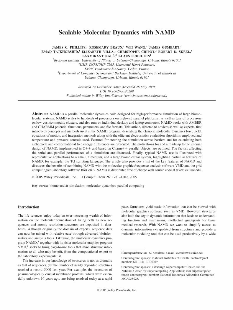
On a molecular scale, the fundamental processing units inthe living cell are often huge in size and function in an evenlarger complex environment. Striking progress has beenachieved in characterizing the immense machines of the cell,such as the ribosome, at the atomic level. Advances in biomed-icine demand tools to model these machines to understand theirfunction and their role in maintaining the health of cells. Ac-cordingly, the purpose of NAMD is to enable high-performanceclassical simulation of biomolecules in realistic environmentsof 100,000 atoms or more. The progress made in this regard isillustrated in Figure 1. A decade ago in its first release,3,4

NAMD permitted simulation of a protein–DNA complex en-compassing 36,000 atoms,5 one of the largest simulations car-ried out at the time. The most recent release permitted thesimulation of a protein–DNA complex of 314,000 atoms.6 Toprobe the behavior of this 10-fold larger system, the simulatedperiod actually increased 100-fold as well.

The following article on NAMD is directed to novices andexperts alike. It explains the concepts and algorithms underlyingmodern molecular dynamics (MD) simulations as realized inNAMD, for example, the efficient numerical integration of theNewtonian equations of motion, the use of statistical mechanicsmethods for simulations that control temperature and pressure, theefficient evaluation of electrostatic forces through the particle-mesh Ewald method, the use of steered and interactive MD tomanipulate and probe biomolecular systems and to speed up reac-tion processes, and the calculation of alchemical and conforma-tional free energy differences.

The article describes the design of NAMD and the motivationbehind the design, that is, to permit continuous software develop-ment in view of ever-changing technologies, to utilize parallelcomputers of any size effectively via message driven computation,to run well on platforms from laptops and desktops—whereNAMD is actually used most—to parallel computers with thou-

sands of processors. The article also demonstrates how the user canreadily extend NAMD through the Tcl scripting language andelaborates on the strengths of NAMD in steered and interactiveMD.

To demonstrate the broad utility of NAMD, the article intro-duces three typical applications as they are encountered in modernresearch, involving a small, an intermediate, and a large biomo-lecular system. We emphasize which features of NAMD were usedand which were most helpful in completing the three modelingprojects expeditiously. We also refer readers to tutorial material(available at http://www.ks.uiuc.edu/Training/Tutorials/) that hasbeen proven helpful in NAMD training workshops and universitycourses. In fact, the first application presented below ubiquitinstems directly from the introductory NAMD tutorial. Other tuto-rials—for which a laptop provides sufficient computationalpower—introduce steered MD and simulations of membrane chan-nels, as well as the use of VMD in trajectory analysis.

Finally, a conclusion section summarizes the features ofNAMD that have proven to be most relevant to nonexpert as wellas expert users and describes the great benefits that NAMD gainsfrom its close link to the widely used molecular graphics programVMD, which permits model building as well as trajectory analysis.The integration of NAMD into the grid software BioCoRE is alsomentioned.

Molecular Dynamics Concepts and Algorithms

In this section we outline concepts and algorithms of classical MDsimulations. In these simulations the atoms of a biopolymer moveaccording to the Newtonian equations of motion

m�r��

�r��

Utotal�r�1, r�2, . . . , r�N�, � � 1, 2 . . . N, (1)

where m� is the mass of atom �, r�� is its position, and Utotal is thetotal potential energy that depends on all atomic positions and,thereby, couples the motion of atoms. The potential energy, rep-resented through the MD “force field,” is the most crucial part ofthe simulation because it must faithfully represent the interactionbetween atoms, yet be cast in the form of a simple mathematicalfunction that can be calculated quickly.

Below we introduce first the functional form of the force fieldutilized in NAMD. We then comment on the special problem ofcalculating the Coulomb potential and forces efficiently. The nu-merical integration of (1) is then explained, followed by an outlineof simulation strategies for controlling temperature and pressure.In the case of such simulations, frictional and fluctuating forces areadded to (1) following the principles of nonequilibrium statisticalmechanics. Finally, we describe how external, user-defined forcesare added to simulations to manipulate and probe biomolecularsystems.

Force Field Functions

For an all-atom MD simulation, one assumes that every atomexperiences a force specified by a model force field accounting for

Figure 1. Growth in practical simulation size illustrated by compar-ison of estrogen receptor DNA-binding domain simulation of ref. 5,left, 36,000 atoms simulated over 100 ps, published in 1997, withmultiscale LacI–DNA complex simulation of ref. 6, right, 314,000atoms simulated over 10 ns, published in 2005 and described in theexemplary applications section. [Color figure can be viewed in theonline issue, which is available at www.interscience.wiley.com.]

1782 Phillips et al. • Vol. 26, No. 16 • Journal of Computational Chemistry

the interaction of that atom with the rest of the system. Today, suchforce fields present a good compromise between accuracy andcomputational efficiency. NAMD employs a common potentialenergy function that has the following contributions:

Utotal � Ubond � Uangle � Udihedral � UvdW � UCoulomb. (2)

The first three terms describe the stretching, bending, and torsionalbonded interactions,

Ubond � �bonds i

kibond�ri � r0i�

2, (3)

Uangle � �angles i

kiangle��i � �0i�

2, (4)

Udihedral � �dihedral i

�kidihe�1 � cos�ni�i � �i��, ni 0

kidihe�0i � �i�

2 n � 0, (5)

where bonds counts each covalent bond in the system, angles arethe angles between each pair of covalent bonds sharing a singleatom at the vertex, and dihedral describes atom pairs separated byexactly three covalent bonds with the central bond subject to thetorsion angle � (Fig. 2). An “improper” dihedral term governingthe geometry of four planar, covalently bonded atoms is alsoincluded as depicted in Figure 2.

The final two terms in eq. (2) describe interactions betweennonbonded atom pairs:

UvdW � �i

�j�i

4ij��ij

rij�12

� ��ij

rij�6�, (6)

UCoulomb � �i

�j�i

qiqj

4�0rij, (7)

which correspond to the van der Waal’s forces (approximated bya Lennard–Jones 6–12 potential) and electrostatic interactions,respectively.

In addition to the intrinsic potential described by the force field,NAMD also provides the user with the ability to apply externalforces to the system. These forces may be used to guide the systeminto configurations of interest, as in steered and interactive MD(described below).

For every particle in a given context of bonds, the parameterski

bond, r0i, etc., for the interactions given in eqs. (3)–(5) are laid outin force field parameter files. The determination of these parame-ters is a significant undertaking generally accomplished through acombination of empirical techniques and quantum mechanicalcalculations;7–9 the force field is then tested for fidelity in repro-ducing the structural, dynamic, and thermodynamic properties ofsmall molecules that have been well-characterized experimentally,as well as for fidelity in reproducing bulk properties. NAMD isable to use the parameterizations from both CHARMM7 andAMBER10 force field specifications.

To avoid surface effects at the boundary of the simulatedsystem, periodic boundary conditions are often used in MD sim-ulations; the particles are enclosed in a cell that is replicated toinfinity by periodic translations. A particle that leaves the cell onone side is replaced by a copy entering the cell on the oppositeside, and each particle is subject to the potential from all otherparticles in the system including images in the surrounding cells,thus entirely eliminating surface effects (but not finite-size effects).Because every cell is an identical copy of all the others, all theimage particles move together and need only be represented onceinside the molecular dynamics code.

However, because the van der Waals and electrostatic interac-tions [eqs. (6) and (7)] exist between every nonbonded pair ofatoms in the system (including those in neighboring cells) com-puting the long-range interaction exactly is unfeasible. To performthis computation in NAMD, the van der Waals interaction isspatially truncated at a user-specified cutoff distance. For a simu-lation using periodic boundary conditions, the system periodicity isexploited to compute the full (nontruncated) electrostatic interac-tion with minimal additional cost using the particle-mesh Ewald(PME) method described in the next section.

Full Electrostatic Computation

Ewald summation11 is a description of the long-range electrostaticinteractions for a spatially limited system with periodic boundary

Figure 2. Internal coordinates for bonded interactions: r governs bondstretching; � represents the bond angle term; � gives the dihedralangle; the small out-of-plane angle � is governed by the so-called“improper” dihedral angle .

Scalable Molecular Dynamics with NAMD 1783

conditions. The infinite sum of charge-charge interactions for acharge-neutral system is conditionally convergent, meaning thatthe result of the summation depends on the order in which it istaken. Ewald summation specifies the order as follows:12 sum overeach box first, then sum over spheres of boxes of increasinglylarger radii. Ewald summation is considered more reliable than acutoff scheme,13–15 although it is noted that the artificial period-icity can lead to bias in free energy,16,17 and can artificiallystabilize a protein that should have unfolded quickly.18

Dropping the prefactor 1/4�, the Ewald sum involves thefollowing terms:

EEwald � Edir � Erec � Eself � Esurface, (8)

Edir �1

2 �i, j�1

N

qiqj �n� r

erfc��r�i � r�j � n�r��r�i � r�j � n�r�

� ��i, j��Excluded

qiqj

�r�i � r�j � �� ij�, (9)

Erec �1

2�V �m� 0

exp��2�m� �2/�2�

�m� �2 ��i�1

N

qiexp(2�im� � r�i)�2

, (10)

Eself � ��

��i�1

N

qi2, (11)

Esurface �2�

�2s � 1�V ��i�1

N

qir�i�2

. (12)

Here, qi and r�i are the charge and position of atom i, respectively,and n� r is the lattice vector. For an arbitrary simulation box definedby three independent base vectors a�1, a�2, a�3, one defines n� r �n1a�1 � n2a�2 � n3a�3, where n1, n2, and n3 are integers. ¥denotes a summation over n� r that excludes the n� r � 0 term in thecase i � j; “excluded” denotes the set of atom pairs whose directelectrostatic interaction should be excluded. �� ij denotes the latticevector for the (i, j) pair that minimizes �r�i � r�j � �� ij�. � is aparameter adjusting the workload distribution for direct and recip-rocal sums. s is the dielectric constant of the surroundings of thesimulation box, which is water for most biomolecular systems. Vis the volume of the simulation box. m� is the reciprocal vectordefined as m� � m1b�1 � m2b�2 � m3b�3, where m1, m2, m3 areintegers, and the reciprocal base vectors b�1, b�2, b�3 are defined sothat

a� � � b� � � ��, �, � � 1, 2, 3. (13)

The complementary error function erfc( x) in eq. (9) is

erfc�x� �2

� x

�

e�t2dt. (14)

The Ewald sum in eq. (8) has four terms: direct sum Edir,reciprocal sum Erec, self-energy Eself, and surface energy Esurface.The self-energy term is a trivial constant, while the surface term isusually neglected by assuming the “tin-foil” boundary conditions � �, which is partly due to the dielectric constant of water(s � 80) being much larger than 1. The Ewald sum has a freelychosen parameter �, which can shift the computational load be-tween the direct sum and the reciprocal sum. For a given accuracy,the computationally optimal choice of the parameter leads to a costproportional to N3/ 2 in the standard computation, where N is thenumber of charges in the system.19

The particle–mesh Ewald (PME)20 method is a fast numericalmethod to compute the Ewald sum. NAMD uses the smooth PME(SPME)21 method for full electrostatic computations. The cost ofPME is proportional to N log N and the time reduction is signif-icant even for a small system of several hundred atoms. In PME,the parameter � is chosen so that the major work load is put intothe reciprocal sum while the direct sum is computed by a costproportional to N only. The reciprocal sum is then computed viafast Fourier transform (FFT) after an approximation is made todelegate the computation to a grid scheme. For this purpose, PMEuses an interpolation scheme to distribute the charges, sittinganywhere in real space, to the nodes of a uniform grid as illustratedin Figure 3. SPME uses B-spline functions as the basis functionsfor the interpolation. The continuity of B-spline functions and theirderivatives makes the analytical expression of forces easy toobtain, and reduces the number of FFTs by half compared to theoriginal PME method. In SPME, approximations are made to thepotential only; the force is still the exact derivative of the approx-imated potential. The strict conservation of energy resulting fromthe computed force is crucial and is strongly assisted by maintain-ing the symplecticness of the integrator,22 as discussed furtherbelow.

The PME method can be adopted to compute the electrostaticpotential in real space and has been implemented in VMD (see Fig.4). The feature has been used recently in a ground-breaking sim-ulation to compute transmembrane electrostatic potentials aver-aged over an MD trajectory.23 This feature makes it possible todayto compute average electrostatic potentials from first principlesand to replace previously used heuristic potentials like those de-rived from Poisson–Boltzmann theory.

The PME method does not conserve energy and momentumsimultaneously, but neither does the particle-particle/particle-meshmethod24 or the multilevel summation method.25,26 Momentumconservation can be enforced by subtracting the net force from thereciprocal sum computation, albeit at the cost of a small long-timeenergy drift.

Numerical Integration

Biomolecular simulations often require millions of time steps.Furthermore, biological systems are chaotic; trajectories start-ing from slightly different initial conditions diverge exponen-tially fast and after a few picoseconds are completely uncorre-lated. However, highly accurate trajectories is not normally agoal for biomolecular simulations; more important is a propersampling of phase space. Therefore, for constant energy (NVEensemble) simulations, the key features of an integrator are not


only how accurate it is locally, but also how efficient it is, andhow well it preserves the fundamental dynamical properties,such as energy, momentum, time-reversibility, and symplectic-ness.

The time evolution of a strict Hamiltonian system is symplec-tic.22 A consequence of this is the conservation of phase spacevolume along the trajectory, that is, the enforcement of the Li-ouville theorem (ref. 27, p. 69). To a large extent, the trajectoriescomputed by numerical integrators observing symplecticness rep-resent the solution of a closely related problem that is still Ham-iltonian.28 Because of this, the errors, unavoidably generated by anintegrator at each time step, accumulate imperceptibly slowly,resulting in a very small long-time energy drift, if there is any atall (ref. 22, theorem IX.8.1). Artificial measures to conserve en-ergy, for example, scaling the velocity at each time step so that thetotal energy is constant, lead to biased phase space sampling of theconstant energy surface;29 in contrast, there has been no evidencethat symplectic integrators have this problem.

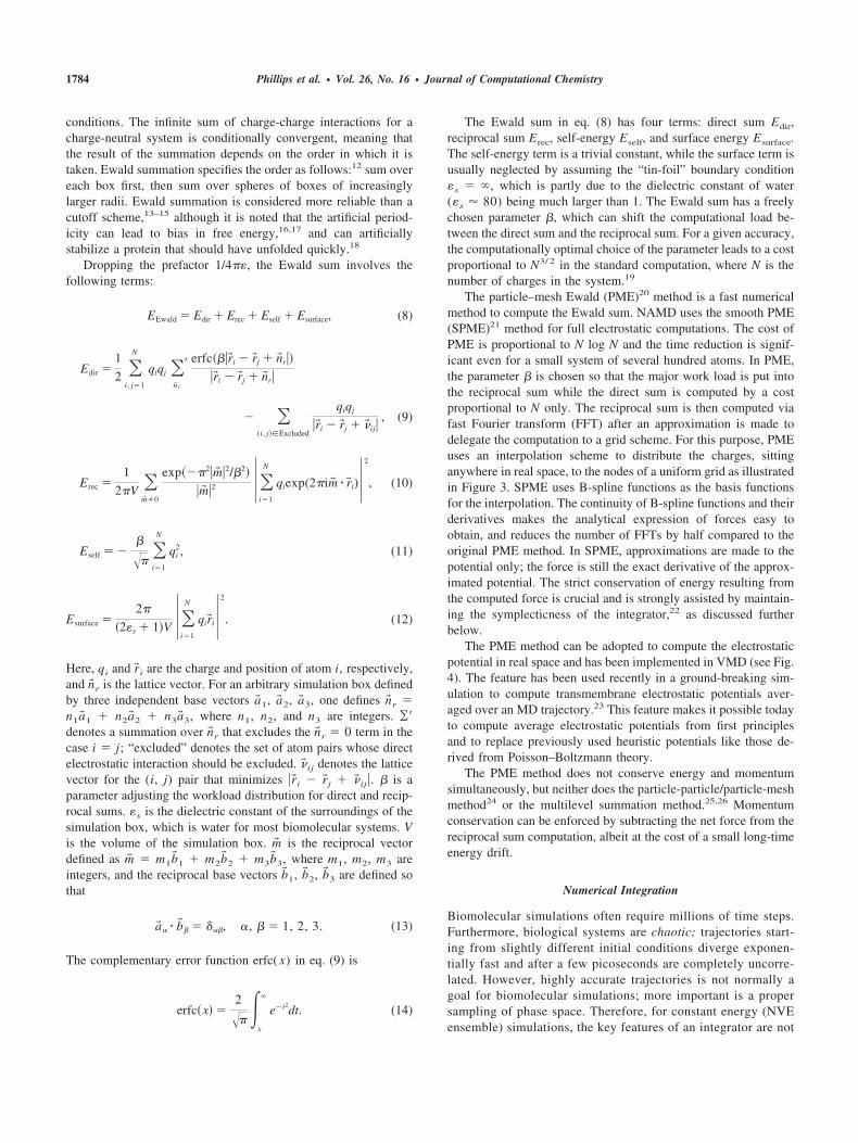
A simple example demonstrates the merit of a symplecticintegrator. For this purpose, the one-dimensional harmonic oscil-lator problem has been numerically integrated, the resulting tra-jectory being shown in Figure 5. We note that the comparison is“unfair” to the symplectic method with respect to both accuracy( t2 local error for the symplectic method vs. t5 for the Runge–Kutta method, where t is the time step), and computational effort(single force evaluation per time step for the symplectic method vs.four force evaluations for the Runge–Kutta method). Nevertheless,the symplectic method shows superior long-time stability.

NAMD uses the Verlet method (ref. 31, section 4.2.3) for NVEensemble simulations. The “velocity-Verlet” method obtains theposition and velocity at the next time step (rn�1, vn�1) from thecurrent one (rn, vn), assuming the force Fn � F(rn) is alreadycomputed, in the following way:

“half-kick” vn�1/ 2 � vn � M�1Fn � t/2,

“drift” rn�1 � rn � vn�1/ 2 t,

“compute force” Fn�1 � F�rn�1�,

“half-kick” vn�1 � vn�1/ 2 � M�1Fn�1 � t/2.

Here, M is the mass. The Verlet method is symplectic and timereversible, conserves linear and angular momentum, and requiresonly one force evaluation for each time step. For a fixed timeperiod, the method exhibits a (global) error proportional to t2.

More accurate (higher order) methods are desirable if they canincrease the time step per force evaluation. Higher order Runge–Kutta type methods, symplectic or not, are not suitable for biomo-lecular simulations because they require several force evaluationsfor each time step and force evaluation is by far the most time-consuming task in molecular dynamics simulations. Gear typepredictor–corrector methods,32 or linear multistep methods in gen-eral, are not symplectic (ref. 22, theorem XIV.3.1). No symplecticmethod has been found as yet that is both more accurate than theVerlet method and as practical for biomolecular simulations.

NAMD employs a multiple-time-stepping13,33,34 method toimprove integration efficiency. Because the biomolecular interac-tions collected in eq. (2) generally give rise to several differenttime scales characteristic for biomolecular dynamics, it is naturalto compute the slower-varying forces less frequently than fastervarying ones in molecular dynamics simulations. This idea isimplemented in NAMD by three levels of integration loops. Theinner loop uses only bonded forces to advance the system, themiddle loop uses Lennard–Jones and short-range electrostaticforces, and the outer loop uses long-range electrostatic forces. Wenote that the method implemented in NAMD is symplectic andtime reversible.

The longest time step for the multiple time-stepping method islimited by resonance.35 When good energy conservation is neededfor NVE ensemble simulations we recommend choosing 2 fs, 2 fs,and 4 fs as the inner, middle, and outer time steps if rigid bonds tohydrogen atoms are used; or 1 fs, 1 fs, and 3 fs if bonds to

Figure 3. In PME, a charge (denoted by an empty circle with label“q” in the figure) is distributed over grid (here a mesh in two dimen-sions) points with weighting functions chosen according to the dis-tance of the respective grid points to the location of the charge.Positioning all charges on a grid enables the application of the FFTmethod and significantly reduces the computation time. In real appli-cations, the grid is three-dimensional.

Figure 4. Smoothed electrostatic potential of decalanine in vacuum ascalculated with the PME plugin of VMD. Atoms are colored by charge(blue is positive, red is negative). The helix dipole is clearly visiblefrom the two potential isosurfaces �20kBT/e (blue, left lobe) and�20kBT/e (red, right lobe). [Color figure can be viewed in the onlineissue, which is available at www.interscience.wiley.com.]


hydrogen are flexible.36 More aggressive time steps may beused for NVT or NPT ensemble simulations, for example, 2 fs,2 fs, and 6 fs with rigid bonds and 1 fs, 2 fs, and 4 fs without.Using multiple time stepping can increase computational effi-ciency by a factor of 2.

NVT and NPT Ensemble Simulations

A fundamental requirement for an integrator is to generate thecorrect ensemble distribution for the specified temperature andpressure in an appropriate way. For this purpose the Newtonianequations of motion (1) should be modified “mildly” so that thecomputed short-time trajectory can still be interpreted in a con-ventional way. To generate the correct ensemble distribution, thesystem is coupled to a reservoir, with the coupling being eitherdeterministic or stochastic. Deterministic couplings generally havesome conserved quantities (similar to total energy), the monitoringof which can provide some confidence in the simulation. NAMDuses a stochastic coupling approach because it is easier to imple-ment and the friction terms tend to enhance the dynamical stability.

The (stochastic) Langevin equation37 is used in NAMD togenerate the Boltzmann distribution for canonical (NVT) ensemblesimulations. The generic Langevin equation is

Mv � F�r� � �v � 2�kBT

MR�t�, (15)

where M is the mass, v � r is the velocity, F is the force, r is theposition, � is the friction coefficient, kB is the Boltzmann constant,T is the temperature, and R(t) is a univariate Gaussian randomprocess. Coupling to the reservoir is modeled by adding the fluc-tuating (the last term) and dissipative (��v term) forces to the

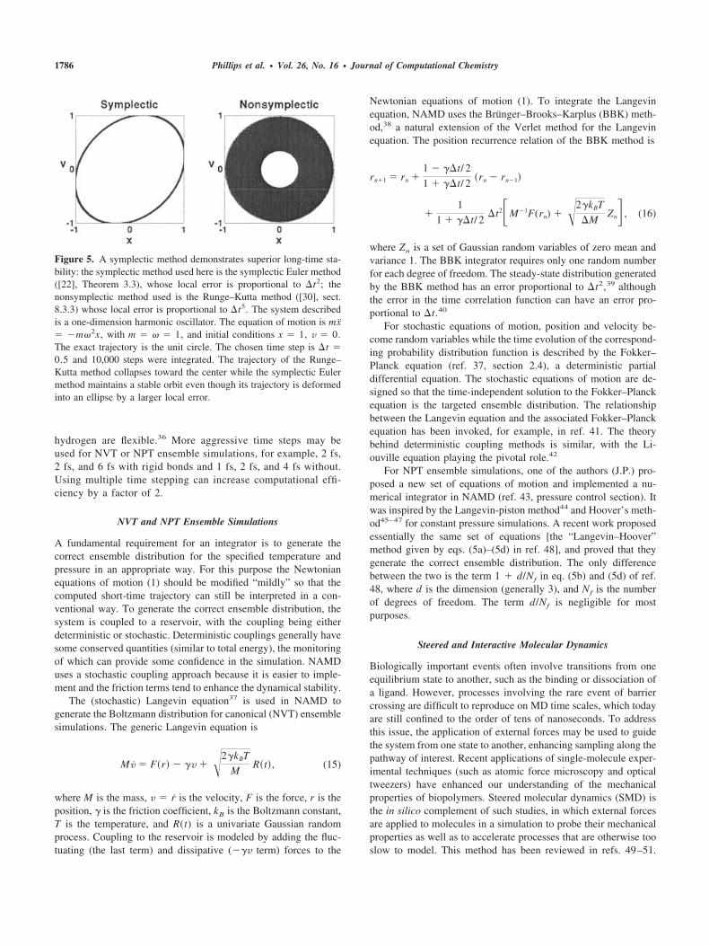
Newtonian equations of motion (1). To integrate the Langevinequation, NAMD uses the Brunger–Brooks–Karplus (BBK) meth-od,38 a natural extension of the Verlet method for the Langevinequation. The position recurrence relation of the BBK method is

rn�1 � rn �1 � � t/ 2

1 � � t/ 2�rn � rn�1�

�1

1 � � t/ 2 t2�M�1F(rn) � 2�kBT

MZn� , (16)

where Zn is a set of Gaussian random variables of zero mean andvariance 1. The BBK integrator requires only one random numberfor each degree of freedom. The steady-state distribution generatedby the BBK method has an error proportional to t2,39 althoughthe error in the time correlation function can have an error pro-portional to t.40

For stochastic equations of motion, position and velocity be-come random variables while the time evolution of the correspond-ing probability distribution function is described by the Fokker–Planck equation (ref. 37, section 2.4), a deterministic partialdifferential equation. The stochastic equations of motion are de-signed so that the time-independent solution to the Fokker–Planckequation is the targeted ensemble distribution. The relationshipbetween the Langevin equation and the associated Fokker–Planckequation has been invoked, for example, in ref. 41. The theorybehind deterministic coupling methods is similar, with the Li-ouville equation playing the pivotal role.42

For NPT ensemble simulations, one of the authors (J.P.) pro-posed a new set of equations of motion and implemented a nu-merical integrator in NAMD (ref. 43, pressure control section). Itwas inspired by the Langevin-piston method44 and Hoover’s meth-od45–47 for constant pressure simulations. A recent work proposedessentially the same set of equations [the “Langevin–Hoover”method given by eqs. (5a)–(5d) in ref. 48], and proved that theygenerate the correct ensemble distribution. The only differencebetween the two is the term 1 � d/Nf in eq. (5b) and (5d) of ref.48, where d is the dimension (generally 3), and Nf is the numberof degrees of freedom. The term d/Nf is negligible for mostpurposes.

Steered and Interactive Molecular Dynamics

Biologically important events often involve transitions from oneequilibrium state to another, such as the binding or dissociation ofa ligand. However, processes involving the rare event of barriercrossing are difficult to reproduce on MD time scales, which todayare still confined to the order of tens of nanoseconds. To addressthis issue, the application of external forces may be used to guidethe system from one state to another, enhancing sampling along thepathway of interest. Recent applications of single-molecule exper-imental techniques (such as atomic force microscopy and opticaltweezers) have enhanced our understanding of the mechanicalproperties of biopolymers. Steered molecular dynamics (SMD) isthe in silico complement of such studies, in which external forcesare applied to molecules in a simulation to probe their mechanicalproperties as well as to accelerate processes that are otherwise tooslow to model. This method has been reviewed in refs. 49–51.

Figure 5. A symplectic method demonstrates superior long-time sta-bility: the symplectic method used here is the symplectic Euler method([22], Theorem 3.3), whose local error is proportional to t2; thenonsymplectic method used is the Runge–Kutta method ([30], sect.8.3.3) whose local error is proportional to t5. The system describedis a one-dimension harmonic oscillator. The equation of motion is mx� �m�2x, with m � � � 1, and initial conditions x � 1, v � 0.The exact trajectory is the unit circle. The chosen time step is t �0.5 and 10,000 steps were integrated. The trajectory of the Runge–Kutta method collapses toward the center while the symplectic Eulermethod maintains a stable orbit even though its trajectory is deformedinto an ellipse by a larger local error.


With advances in available computer power, steering forces canalso be applied interactively, instead of in batch mode; we call thistechnique Interactive Molecular Dynamics (IMD).52,53 Externalforces have been applied using NAMD in a variety of ways to adiverse set of systems, yielding new information about the me-chanics of proteins,54 for instance in refs. 6, 55–67 and otherstudies reviewed in ref. 51. We expect that most molecular dy-namics simulations in the future will be of the steered type. Thisexpectation stems from an analogy to experimental biophysics:although many experiments provide unaltered images of biologicalsystems, more experiments investigate systems through well-de-signed perturbations by physical or chemical means.

SMD

Steered MD may be carried out with either a constant force appliedto an atom (or set of atoms) or by attaching a harmonic (spring-like) restraint to one or more atoms in the system and then varyingeither the stiffness of the restraint67 or the position of the re-straint68–70 to pull the atoms along. Other external forces orpotentials can also be used, such as constant forces or torquesapplied to parts of the system to induce rotational motion of itsdomains. NAMD provides built-in facilities for applying a varietyof external forces, including the automated application of movingconstraints. In SMD, the direction of the applied force is chosen inadvance, specified through a few simple lines in an NAMD con-figuration file. More flexible force schemes can be realized withinNAMD through scripting.

As a computational technique, SMD bears similarities to themethod of umbrella sampling,71,72 which also seeks to improve thesampling of a particular degree of freedom in a biomolecularsystem; however, while umbrella sampling requires a series ofequilibrium simulations, SMD simulations apply a constant ortime-varying force that results in significant deviations from equi-librium. In consequence, the results of the SMD dynamics have tobe analyzed from an explicitly nonequilibrium viewpoint.54 SMDalso permits new types of simulations that are more naturallyperformed and understood as out-of-equilibrium processes.

In constant-force SMD, the atoms to which the force is appliedare subject to a fixed, constant force in addition to the force fieldpotential. The affected atoms are specified through a flag in themolecular coordinates (PDB) file, and the force vector is specifiedin the NAMD configuration. Intermediates found through con-stant-force SMD simulations may be modeled using the theory ofmean first passage times for a barrier-crossing event.73,74 Typicalapplied forces range from tens to a thousand picoNewtons (pN).75

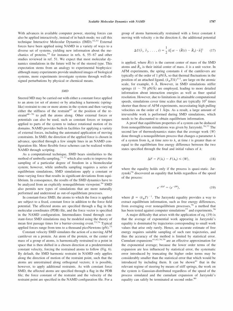
Constant velocity SMD simulates the action of a moving AFMcantilever on a protein. An atom of the protein, or the center ofmass of a group of atoms, is harmonically restrained to a point inspace that is then shifted in a chosen direction at a predeterminedconstant velocity, forcing the restrained atoms to follow (Fig. 6).By default, the SMD harmonic restraint in NAMD only appliesalong the direction of motion of the restraint point, such that theatoms are unrestrained along orthogonal vectors; it is possible,however, to apply additional restraints. As with constant forceSMD, the affected atoms are specified through a flag in the PDBfile; the force constant of the restraint and the velocity of therestraint point are specified in the NAMD configuration file. For a

group of atoms harmonically restrained with a force constant kmoving with velocity v in the direction n� , the additional potential

U�r�1, r�2, . . . , t� �1

2k�vt � �R� �t� � R� 0� � n� �2 (17)

is applied, where R� (t) is the current center of mass of the SMDatoms and R� 0 is their initial center of mass. n� is a unit vector. InAFM experiments, the spring constants k of the cantilevers aretypically of the order of 1 pN/Å, so that thermal fluctuations in theposition of an attached ligand, (kBT/k)1/ 2, are large on the atomicscale, for example, 6 Å. However, in SMD simulations stiffersprings (k � 70 pN/Å) are employed, leading to more detailedinformation about interaction energies as well as finer spatialresolution. However, due to limitations in attainable computationalspeeds, simulations cover time scales that are typically 105 timesshorter than those of AFM experiments, necessitating high pullingvelocities on the order of 1 Å/ps. As a result, a large amount ofirreversible work is performed during SMD simulations, whichneeds to be discounted to obtain equilibrium information.

A proof that equilibrium properties of a system can be deducedfrom nonequilibrium simulations was given by Jarzynski.76,77 Thesecond law of thermodynamics states that the average work �W�done through a nonequilibrium process that changes a parameter �of a system from �0 at time zero to �t at time t is greater than orequal to the equilibrium free energy difference between the twostates specified through the final and initial values of �:

F � F��t� � F��0� � �W�, (18)

where the equality holds only if the process is quasi-static. Jar-zynski76 discovered an equality that holds regardless of the speedof the process:

e�� F � �e��W�, (19)

where � � (kBT)�1. The Jarzynski equality provides a way toextract equilibrium information, such as free energy differences,from averaging over nonequilibrium processes,76 a method thathas been tested against computer simulations77 and experiments.78

A major difficulty that arises with the application of eq. (19) isthat the average of exponential work appearing in Jarzynski’sequality is dominated by trajectories corresponding to small workvalues that arise only rarely. Hence, an accurate estimate of freeenergy requires suitable sampling of such rare trajectories, andthus the accuracy of the method is limited by statistical error.Cumulant expansions41,62,76,79 are an effective approximation forthe exponential average; because the lower order terms of theexpansion are less influenced by statistical error, the systematicerror introduced by truncating the higher order terms may beconsiderably smaller than the statistical error that which would beintroduced by including them. It can be shown41 that in therelevant regime of steering by means of stiff springs, the work onthe system is Gaussian-distributed regardless of the speed of theprocess simulated and the cumulant expansion of Jarzynski’sequality can safely be terminated at second order.80


Application of the Jarzynski identity is comparable in effi-ciency to the umbrella sampling method.81 However, the analysisinvolved in the SMD method is simpler than that involved inumbrella sampling in which one needs to solve coupled nonlinearequations for the weighted histogram analysis method.31,54,82,83 Inaddition, the application of the Jarzynski identity has the advantageof uniform sampling of a reaction coordinate. Whereas in umbrellasampling a reaction coordinate is locally sampled nonuniformlyproportional to the Boltzmann weight, in SMD a reaction coordi-nate follows a guiding potential that moves with a constant veloc-ity and, hence, is sampled almost uniformly (computing time isuniformly distributed over the given region of the reaction coor-dinate). This is particularly beneficial when the potential of meanforce (essentially, the free energy profile along the reaction coor-dinate) contains narrow barrier regions as in ref. 62. In such cases,a successful application of umbrella sampling depends on anoptimal choice of biasing potentials, whereas nonequilibrium ther-modynamic integration appears to be more robust.31 However,umbrella sampling is a general method that can be applied to avariety of reaction coordinates, including complex ones like thoseinvolved in large conformational changes in proteins.84

NAMD also provides the facility for the user to apply othertypes of external forces to a system. In a technique related to SMD,torques may be applied to induce the rotation of a protein domain.As with SMD, this is implemented in NAMD through a simplespecification in the configuration file and does not require addi-tional programming on the part of the researcher. This techniquehas already been successfully used to study the rotation of the Fo

domain of ATPase.85 The application of more sophisticated exter-nal forces are readily implemented through the NAMD “Tclforces” interface, which allows the user to specify position- andtime-dependent forces to be computed at each time step. Thistechnique has recently been used to mimic the effect of membranesurface tension on a mechanosensitive channel59 and to model theinteraction of the lac repressor protein (modeled in atomic-leveldetail) with DNA described by an elastic rod that exerts forces onthe protein.6,86

IMD

By using NAMD in conjunction with the molecular graphicssoftware VMD, steering forces can be applied in an interactivemanner, rather than only in batch mode.52 For this purpose, VMDis linked to a NAMD simulation running on the same machine ora remote cluster. This arrangement permits an investigator to viewa running simulation and to apply forces based on real-time infor-mation about the progress of the simulation (such as visual infor-mation or force feedback through a haptic device). The researcheris then able to explore the mechanical properties of the system ina direct, hands-on manner, using her scientific intuition to guidethe simulation via a mouse or haptic device. This method hasalready been used in biomolecular research, for instance, to studythe selectivity and regulation of the membrane channel proteinGlpF and the enzyme glycerol kinase.53 Setting up an IMD sim-ulation is a straight-forward process that can be done on anycomputer.

The IMD haptic interface52 consists of three primary compo-nents: a haptic device to provide translational and orientationalinput as well as force feedback to the user’s hand; NAMD tocalculate the effect of applied forces via molecular dynamics; andVMD to display results (Fig. 7). VMD communicates with thehaptic device via a server87 that controls the haptic environmentexperienced by the user, as described in ref. 52. The scheme ofsplitting the haptic, visualization, and simulation components intothree communicating, asynchronous processes has been employedsuccessfully,52,88 and permits all three components to run at topspeed, maximizing the responsiveness of the system. IMD requires

Figure 6. Constant velocity pulling in a one-dimensional case. Thedummy atom is colored red, and the SMD atom blue. As the dummyatom moves at constant velocity, the SMD atom experiences a forcethat depends linearly on the distance between both atoms. [Color figurecan be viewed in the online issue, which is available at www.interscience.wiley.com.]

Figure 7. In IMD, the user applies forces to atoms in the simulationvia a force-feedback haptic device.


efficient network communication between the visualization front-end and the MD back-end. Although the network bandwidth re-quirements for performing IMD are quite low relative to thecomputational demands, latency is a major concern as it has adirect impact on the responsiveness of the system. IMD usescustom networking code in NAMD and VMD to transfer atomiccoordinates and steering forces efficiently.

To make molecular motion as described by MD perceptible tothe IMD user through the haptic device, the quantities arising inthe generic equation of motion governing the molecular response(represented below by Roman characters) and the haptic response(denoted by Greek characters),

md2x

dt2 � f, �d2�

d�2 � � (20)

must be related through suitable scaling factors. Molecular motionprobed is typically extended over distances of x � 1 Å, moleculartime scales covered are typically t � 1 ps, and external forcesacting on molecular moieties should not exceed f � 1 nN so as notto overwhelm inherent molecular forces. By contrast, the hapticdevice is characterized by length resolution of � � 1 cm and cangenerate a force of � � 1 N or more; t � 1 ps of dynamicsrequires � � 1 s or more to compute. The interface between thehaptic device and NAMD thus introduces the scaling factors

Sx � �/x � 108, St � � /t � 1012, Sf � �/f � 109, (21)

Multiplying the molecular equation of motion in eq. (20) by thefactor SfSx/St

2 gives

SfSx

St2 m

d2x

dt2 � Sfmd2�

d�2 �SfSx

St2 f �

Sx

St2 �. (22)

From this we can conclude

SfSt2

Sxm

d2�

d�2 � �. (23)

Comparison with the haptic equation of motion in eq. (20) suggeststhat the effective mass felt by the haptic device, and hence, by theuser is

� �SfSt

2

Sxm. (24)

The molecular moieties to be moved through external forces havetypical masses of (e.g., for glycerol moved through a membranechannel53) of m � 180 amu or m � 3 � 10�25 kg. From eq. (21)we conclude then that the effective mass felt by the user throughthe haptic device is 3 kg; the user does not sense strong inertialeffects, and can readily manipulate the biomolecular system. IMDcan also be carried out without force feedback, using a standardmouse to steer the simulated system.

To assist users of NAMD with IMD, AutoIMD89 has beendeveloped. AutoIMD permits the researcher to use the graphical

interface provided by VMD to run an MD simulation based on aselection of atoms. The simulation can then be visualized in realtime in the VMD graphics window. Forces may be applied witheither a mouse or a haptic device by the user (as described above),or statically as in traditional SMD. Rather than carrying out asimulation of the entire molecule, AutoIMD performs a rapid MDsimulation by dividing the system into three parts: a “moltenzone,” where the atoms are allowed to move freely; a surrounding“fixed zone,” in which the atoms are included in the simulation(and exert forces on the molten zone), but are held fixed; and an“excluded zone,” which is entirely disregarded in the AutoIMDsimulation. In this way, AutoIMD may be used to inspect andperform energy minimizations on parts of the system that havebeen manipulated (e.g., through mutations or IMD), giving theresearcher real-time feedback on the simulation.

SMD and IMD simulations differ in fundamental ways, andmay be fruitfully combined. In SMD, the specification of theexternal forces is developed based on the researcher’s understand-ing of the biological and structural properties of the system. TheSMD simulation is carried out with the weakest force possible toinduce the necessary change in an affordable length of simulationtime, and the analysis of the simulation data relates the forceapplied to the progress of the system along the chosen reactionpath. In contrast, IMD simulations are unplanned, allowing theresearcher to toy with the system, exploring the degrees of free-dom. Because the simulations need to be rapid—completed inminutes rather than days or weeks—the applied forces are ex-tremely large, and the simulations are too rough to produce datasuitable for an accurate analysis of molecular properties. Thetechniques can be combined: in the first stage, the researcher usesIMD to generate and test hypotheses for reaction mechanisms or toaccelerate substrate transport, docking, and other mechanisms thatare difficult to cast into numerical descriptions; in the second stage,the researcher carries out further MD or SMD simulations buildingon the hypothesized mechanisms or configurations from the IMDinvestigation.

Free Energy Calculations

In addition to propagating the motion of atoms in time, MD canalso be used to generate an ensemble of configurations, from whichthermodynamic quantities like free energy differences, F, can becomputed. In a nutshell, there are three possible routes for thecalculation of F: (1) estimate the relevant probability distribu-tion, �[U(r�1, . . . , r�N)], from which a free energy difference maybe inferred via �1/� ln �[U(r�1, . . . , r�N)]/�0, where �0 denotes anormalization term: (2) compute the free energy difference di-rectly; and (3) calculate the free energy derivative, d F(�)/d�,along some order parameter (collective coordinate), �, consistentwith an average force,90 and integrate the latter to obtain F.

The popular umbrella sampling method,71,72 whereby the prob-ability to find the system along a given reaction coordinate issought, falls evidently into the first category. One blatant short-coming of this scheme, however, lies in the need to guess theexternal potential or bias that is necessary to overcome the barriersof the free energy landscape—an issue that may rapidly becomeintricate in the case of qualitatively new problems. In this section,


we shall focus on the second and the third classes of approachesfor determining free energy differences.

The first approach, available in NAMD since version 2.4, isfree energy perturbation (FEP),91 an exact method for the directcomputation of relative free energies. FEP offers a convenientframework for performing “alchemical transformations,” or insilico site-directed mutagenesis of one chemical species into an-other.

Description of intermolecular association or intramolecular de-formation in complex molecular assemblies requires an efficientcomputational tool, capable of rapidly providing precise free en-ergy profiles along some ordering parameter, �, in particular whenlittle is known about the underlying free energy behavior of theprocess. A fast and accurate scheme, pertaining to the third cate-gory of methods, is introduced in NAMD version 2.6 to determinesuch free energy profiles, F(�). This scheme relies upon theevaluation of the average force acting along the chosen orderparameter, �, in such a way that no apparent free energy barrierimpedes the progress of the system along the latter.92,93

The efficiency of the free energy algorithm represents only onefacet of the overall performance of the free energy calculation,which to a large extent, relies on the ability of the core MDprogram to supply configurations and forces in rigorous thermo-dynamic ensembles and in a time-bound fashion. The methodologydescribed hereafter has been implemented in NAMD and operateswith nearly no extra cost compared to a standard MD simulation.

Alchemical Transformations

Contrary to the worthless piece of lead in the hands of the pro-verbial alchemist, the potential energy function of the computa-tional chemist is sufficiently malleable to be altered seamlessly,thereby allowing the thermodynamic properties of a system to berelated to those of a slightly modified one, such as a chemicallymodified protein or ligand, through the difference in the corre-sponding intermolecular potentials.

The free energy difference between a reference state, a, and atarget state, b, can be expressed in terms of the ratio of theircorresponding partition functions. Using the well-known relation-ship between partition function Z and free energy F, Z � exp[�F/k8T], along with the property Z � ZkinZpot where Zkin and Zpot arethe partition functions for kinetic and potential energy, respec-tively, one can express F a3b � Fb � Fa as:

Fa3b � �1

�ln

� exp��Ub�r�1, . . . , r�N��dr�1 . . . dr�N

� exp��Ua�r�1, . . . , r�N��dr�1 . . . dr�N. (25)

Here Ua and Ub are the potential energy functions for states a andb, respectively. One can write eq. (25) Fa3b ��(1/�)ln{�exp[��(Ub(�)�Ua(�))]exp[��Ua(�)]dx/�exp[��Ua(�)]dx} where� � r�1, . . . , r�N . Defining the average, Boltzmann-weighted relative tothe potential Ua, that is, weighted over configurations representa-tive of the reference state a, �f�a � �f(�)exp[��Ua(�)]dx/�exp[��Ua(�)]dx, one can state:

Fa3b � �1

�ln�exp��Ub�r�1, . . . , r�N� � Ua�r�1, . . . , r�N��a.

(26)

This is the celebrated FEP equation.91 In principle, eq. (26) isexact in the limit of infinite sampling. In practice, however, on thebasis of finite-length simulations, it only provides accurate esti-mates for small changes between a and b. This condition does notimply that the free energies characteristic of a and b be sufficientlyclose, but rather that the corresponding configurational ensemblesoverlap to a large degree to guarantee the desired accuracy. Forexample, although the hydration free energy of benzene is only�0.4 kcal/mol, insertion of a benzene molecule in bulk waterconstitutes too large a perturbation to fulfill the latter requirementin a single-step transformation. If such is not the case, the pathwayconnecting state a to state b is broken down into N intermediate,not necessarily physical states, �k (a � �1 � 0 and b � �N �1), so that the Helmholtz free energy difference reads:

Fa3b � �1

� �k�1

N�1

ln�exp��U�r�1, . . . , r�N; �k�1�

� U�r�1, . . . , r�N; �k��k. (27)

Here the potential energy is not only a function of the spatialcoordinates, but also of the parameter � that connects the referenceand the target states. Perturbation of the chemical system by meansof �k may be achieved by scaling the relevant nonbonded forcefield parameters of appearing, vanishing, or changing atoms, in thespirit of turning lead into gold.

In NAMD, the topologies characteristic of the initial state, a,and the final state, b, coexist, yet without interacting. This impliesthat, as a preamble to the free energy calculation, a hybrid topol-ogy has to be defined with an appropriate exclusion list to preventinteractions between those atoms unique to state a and thoseunique to state b. In lieu of altering the nonbonded parameters, theinteraction of the perturbed molecular fragments with their envi-ronment is scaled as a function of �k:

U�r�1, . . . , r�N; �k� � �kUb�r�1, . . . , r�N�

� �1 � �k�Ua�r�1, . . . , r�N�. (28)

This scheme is referred to as the dual-topology paradigm.94

In a number of MD programs, FEP is implemented as an extralayer, implying that free energy differences are computed a pos-teriori by looping over a previously generated trajectory. InNAMD, the potential energies representative of the reference state,�k, and the target state, �k�1, are evaluated concurrently “on thefly” at little additional cost and the ensemble average of eq. (27) isupdated continuously.

“Alchemical transformations” may be applied to a variety ofchemically and biologically relevant systems, offering, in ad-dition to a free energy difference, atomic-level insight into thestructural modifications entailed by the perturbation. In Figure8, in silico site-directed mutagenesis experiments are proposedfor the transmembrane domain of glycophorin A (GpA) in anattempt to pinpoint those residues responsible for �-helixdimerization. Leu75 and Ile76 are perturbed into alanine follow-ing the depicted thermodynamic cycle. The first point mutation,L75A, yields a free energy change of �13.9 � 0.3 and �28.8 �


0.5 kcal/mol in the free and in the bound state, respectively,which, put together, corresponds to a net free energy change of�1.0 � 0.6 kcal/mol (experimental estimate:95 �1.1 � 0.1kcal/mol). The second point mutation, I76A, led to a freeenergy change of �4.9 � 0.3 and �8.4 � 0.4 kcal/mol, in thesingle helix and in the dimer, respectively, that is, a net changeof �1.4 � 0.5 kcal/mol (experimental estimate:95 �1.7 � 0.1kcal/mol). Aside from the remarkable agreement between the-ory and experiment, these free energy calculations confirm thatreplacement of bulky nonpolar side chains like leucine orisoleucine by alanine disrupts the �-helical dimer through a lossof van der Waals interactions.96

Overcoming Free Energy Barriers Using an AdaptiveBiasing Force

The sizeable number of degrees of freedom described explicitly instatistical simulations of large molecular assemblies, in particularthose of both chemical and biological interest, rationalizes the need

for a compact description of thermodynamic properties. Free en-ergy profiles offer a suitable framework that fulfills this require-ment by providing the dependence of the free energy on the chosendegrees of freedom �. Determination of such free energy profiles,under the sine qua non condition that some key degree of freedom�, for example, a reaction coordinate, can be defined, however,remains a daunting task from the perspective of numerical simu-lations. In the context of Boltzmann sampling of the phase space,overcoming the high free energy barriers that separate thermody-namic states of interest is a rare event that is unlikely to occur onthe time scales amenable to MD simulation.

An important step forward on the road towards an optimalsampling of the phase space along a chosen collective coordinate,�, has been made recently. In a nutshell, this new method relies onthe continuous application of a dynamically adapted biasing forcethat compensates the current estimate of the free energy, thusvirtually erasing the roughness of the free energy landscape as thesystem progresses along �.92 To reach this goal, the average force

Figure 8. Homodimerization of the transmembrane (TM) domain of glycophorin A (GpA): (a) Contactsurface of the two �-helices forming the TM domain of GpA. The strongest contacts are observed in theheptad of amino acids, Leu75, Ile76, Gly79, Val80, Gly83, Val84, and Thr87. Residue Leu75, whichparticipates in the association of the two �-helices through dispersive interactions, is featured astransparent van der Waals spheres. (b) Free energy profile delineating the reversible dissociation of thetwo �-helices, obtained using an adaptive biasing force. The ordering parameter, �, corresponds to thedistance separating the center of mass of the TM segments. The entire pathway was broken down into 10windows, in which up to 15 ns of MD sampling was performed, corresponding to a total simulation timeof 125 ns. (c) Thermodynamic cycle utilized to perform the “alchemical transformation” of residues Leu75

and Ile76 into alanine, demonstrating the participation of these amino acids in the homodimerization of thetwo �-helices. The left vertical leg of the cycle represents the transformation in a single �-helix from thewild-type (WT) to the mutant form. The right vertical leg denotes a simultaneous point mutation in thetwo interacting �-helices. Using the notation of the figure, the free energy difference arising from thisperturbation is equal to G2

mutation � 2 G1mutation. Each leg of the thermodynamic cycle consists of 50

intermediate states and a total MD sampling of 6 ns. For clarity, the environment of the �-helical dimer,formed by a dodecane slab in equilibrium between two lamellae of water, is not shown. [Color figure canbe viewed in the online issue, which is available at www.interscience.wiley.com.]


acting on �, �F��, is evaluated from an unconstrained MD simu-lation:93

dA��

d�� U(r�1, . . . , r�N)

��

1

�

� ln�J��

��

� ��F��, (29)

where �J� denotes the determinant of the Jacobian for the trans-formation from Cartesian to generalized coordinates, which is anecessary modification of metric, given that {r�1, . . . , r�N} and �are not independent variables. The specific form of �J� is aninherent function of the coordinate, �, chosen to advance thesystem.

In the course of the simulation in NAMD, the force, F�, actingalong the ordering parameter, �, is accrued in small bins, therebysupplying an estimate of the derivative dA(�)/d�. The so calledadaptive biasing force (ABF), F� ABF � ��F��r�, is determinedin such a way that, when applied to the system, it yields aHamiltonian in which no average force is exerted along �. As aresult, all values of � are sampled with an equal probability, whichin turn, dramatically improves the accuracy of the calculated freeenergies. The approach further entails that progression of thesystem along � is fully reversible and limited solely by its self-diffusion properties. At this stage, it should be clearly understoodthat whereas the ABF method enhances sampling along �, itsability to supply a perfectly uniform probability distribution of thesystem over the entire range of � values may be impeded bypossible orthogonal degrees of freedom.

We have chosen to introduce the average force method in NAMDwithin the convenient framework of unconstrained MD,93 in whichthe coordinate, � is unconstrained, but other degrees of freedom, suchas bond lengths, can be constrained. Either constraint forces must betaken into account in F�, as they are in NAMD version 2.6, or it willbe crucial to ascertain that no Cartesian coordinate appears simulta-neously in a constrained degree of freedom and in the derivative�U(r�1, . . . , r�N)/�� of eq. (29).

The implementation of the ABF scheme in NAMD providesreaction coordinates such as a distance between subgroups of atoms orlength along a specified direction in cartesian space. Previous appli-cations include, the intramolecular folding of a short peptide, thepartitioning of small solutes across an aqueous interface, and theintermolecular association of neutral and ionic species.92,93

The �-helical dimerization of GpA represents an interestingapplication of the method, whereby the reversible dissociation—rather than the association, for obvious cost-effectiveness rea-sons—is carried out, using the distance separating the center ofmass of the trans-membrane segments as the reaction coordinate.The free energy profile characterizing this process is shown inFigure 8, and features a deep minimum at 8.2 Å, which corre-sponds to the native, close packing of the �-helices.

As the trans-membrane segments move away from eachother, helix– helix interactions are progressively disrupted, inparticular in the crossing region, thus causing an abrupt in-crease of the free energy, accompanied by a tilt of the two�-helices towards an upright orientation. As the distance be-tween the two trans-membrane segments further increases, thefree energy profile levels off at 21 Å, a separation beyond whichthe dimer is fully dissociated.

A valuable feature offered by NAMD lies in the possibilityto evaluate a posteriori electrostatic and van der Waals forcesfrom an ensemble of configurations. Projection of these forcesonto the coordinate �, and subsequent integration of the formerprovides a deconvolution of the complete free energy profile interms of helix– helix and helix–solvent contributions.

Analysis of these contributions reveals two regimes in theassociation process, driven at large separation by the solvent,which pushes the �-helices together, and at short separation by vander Waals interactions that favor native contacts.96

NAMD Software Design

Just as the intelligent car buyer looks under the hood to understandthe performance and longevity of a particular vehicle, we nowdirect the attention of the reader and potential NAMD user to a fewdesign and implementation details that contribute to the flexibilityand performance of NAMD.

Goals, Design, and Implementation

NAMD was developed to enable ambitious MD simulations ofbiomolecular systems, employing the best technology available toprovide the maximum performance possible to researchers. In thepast decade simulation size and duration have increased dramati-cally. Ten years ago a simulation of 36,000 atoms over 100 ps asreported in ref. 5 was considered very advanced. Today, this statusis reserved for simulations of systems with more than 300,000atoms for up to 100 ns as reported in refs. 6, 23, and 55. Theprogress made is illustrated in Figure 1, comparing the sizes ofsystems reported in refs. 5 and 6. This 1000-fold increase incapability (10-fold in atom count and over 100-fold in simulationlength) has been partially enabled by advances in processor per-formance, with clock rate increases leading the way. However,substantial progress has also resulted from exploiting the factor of100 or more in performance available through the use of massivelyparallel computing, coordinating the efforts of numerous proces-sors to address a single computation.

Looking forward, scientific ambition remains unchecked whileincreases in processor clock rates are constrained by limits on powerconsumption and heat dissipation. This stagnation in CPU speed hasinspired system vendors such as Cray and SGI to incorporate field-programmable gate arrays (FPGAs) into their offerings, promisinggreat performance increases, but only for suitable algorithms that aresubjected to heroic porting efforts (as have been initiated for the forceevaluations used by NAMD). Advances in semiconductor technologywill surpass the limits encountered today, but in the meantime, indus-try has turned to offering greater concurrency to performance-hungryapplications, scaling systems to more processors, and processors tomore cores, rather than to higher clock rates. Indeed, the highest-performance component of a modern desktop is often the 3D graphicsaccelerator, which inexpensively provides an order of magnitudegreater floating point capability than the main processor at a fractionof the clock rate by automatically distributing independent calcula-tions to tens of pipelines, and even across multiple boards. Therefore,high performance and parallel computing will become even moresynonymous than today, with greater industry acceptance and support.


Scientific computing is also facing the perennial “softwarecrisis” that has stalked business information systems for decades.The seminal book by Allen and Tildesley97 could dedicate a fewpages of an appendix to writing efficient FORTRAN-77 code andconsider the reader adequately informed. Developing modernhigh-performance software, however, requires knowledge of ev-erything from parallel decomposition and coordination libraries tothe relative cost of accessing different levels of cache memory.The design of more complex algorithms and numerical methodshas ensured that any useful and successful program is likely tooutlive the machine for which it is originally written, makingportability a necessity. Software is also likely to be used andextended by persons other than the original author, making codereadability and modifiability vital.

Software maintenance activities such as porting and modifica-tion account for the majority of the cost and effort associated witha program during its lifetime. These issues have been addressed inthe development of object-oriented software design, in which theprogrammer breaks the program into “objects” comprising closely-related data (such as the x, y, and z components of a vector) andthe operations that act on it (addition, dot product, cross product,etc.). The objects may be arranged into hierarchies of classes, andan object may contain or refer to other objects of the same ordifferent classes. In this manner, large and complex programs canbe broken down into smaller components with defined interfacesthat can be implemented independently. NAMD is implemented inC��, the most popular and widely supported programming lan-guage providing efficient support for these methods.

Methodology for the development of parallel programs is farfrom mature, with automatically parallelizing compilers and lan-guages still quite limited and most programmers using the Mes-sage Passing Interface (MPI) libraries in combination with C,C��, or Fortran. Although the acceptance of MPI as a crossplat-form standard for parallel software has been of great benefit, theburden on the programmer remains. The first task is to decomposethe problem, which is often simplified by assuming that the pro-cessor count is a power of two or has factors corresponding to thedimensions of a large three-dimensional array. MPI programmingthen requires the explicit sending and receiving of arrays betweenprocessors, much like directing a large and complex game of catch.

NAMD is based on the Charm�� parallel programming sys-tem and runtime library.98 In Charm��, the computation is de-composed into objects that interact by sending messages to otherobjects on either the same or remote processors. These messagesare asynchronous and one sided, that is, a particular method isinvoked on an object whenever a message arrives for it rather thanhaving the object waste resources while waiting for incoming data.This message-driven object programming style effectively hidescommunication latency and is naturally tolerant of the systemnoise that is found on workstation clusters. Charm�� also sup-ports processor virtualization,99 allowing each algorithm to bewritten for an ideal, maximum number of parallel objects that arethen dynamically distributed among the actual number of proces-sors on which the program is run. Charm�� provides thesebenefits even when it is implemented on top of MPI, an option thatallows NAMD to be easily ported to new platforms.

The parallel decomposition strategy used by NAMD is to treatthe simulation cell (the volume of space containing the atoms) as

a three-dimensional patchwork quilt, with each patch of sufficientsize that only the 26 nearest-neighboring patches are involved inbonded, van der Waals, and short-range electrostatic interactions.More precisely, the patches fill the simulation space in a regulargrid and atoms in any pair of non-neighboring patches are sepa-rated by at least the cutoff distance at all times during the simu-lation. Each hydrogen atom is stored on the same patch as the atomto which it is bonded, and atoms are reassigned to patches atregular intervals. The number of patches varies from one to severalhundred and is determined by the size of the simulation indepen-dently of the number of processors. Additional parallelism may begenerated through options that double the number (and have thesize) of patches in one or more dimensions.

When NAMD is run, patches are distributed as evenly aspossible, keeping nearby patches on the same processor when thereare more patches than processors, or spreading them across themachine when there are not. Then, a (roughly 14 times) largernumber of compute objects responsible for calculating atomicinteractions either within a single patch or between neighboringpatches is distributed across the processors, minimizing commu-nication by grouping compute objects responsible for the samepatch together on the same processors. At the beginning of thesimulation, the actual processor time consumed by each computeobject is measured, and this data is used to redistribute computeobjects to balance the workload between processors. This mea-surement-based load balancing100 contributes greatly to the paral-lel efficiency of NAMD.

Using forces calculated by compute objects, each patch isresponsible for integrating the equations of motion for the atoms itcontains. This can be done independently of other patches, butoccasionally requires global data affecting all atoms, such as achange in the size of the periodic cell due to a constant pressurealgorithm. Although the integration algorithm is the clearly visible“outer loop” in a serial program, NAMD’s message-driven designcould have resulted in much obfuscation (as was experienced evenin the simpler NAMD 1.X4). This was averted by using Charm��threads to write a top-level function that is called once for eachpatch at program start and does not complete until the end of thesimulation.10 This design has allowed pressure and temperaturecontrol methods and even a conjugate gradient minimizer to beimplemented in NAMD without writing any new code for parallelcommunication.

Tcl Scripting Interface

NAMD has been designed to be extensible by the end user in thoseareas that have required the most modification in the past and thatare least likely to affect performance or harbor hard-to-detectprogramming errors. The critical force evaluation and integrationroutines that are the core of any molecular dynamics simulationhave remained consistent in implementation as NAMD hasevolved, occasionally introducing improved methods for pressureand temperature control. The greatest demand for modification hasbeen in high-level protocols, such as equilibration and simulatedannealing schedules. An additional demand has been for the im-plementation of experimental and often highly specialized steeringand analysis methods, such as those used to study the rotationalmotion of ATP synthase.85


Flexibility requirements could, in theory, be met by having theend user modify NAMD’s C�� source code, but this is undesir-able for several reasons. Any users with special needs would haveto maintain their own “hacked” version of the source code, whichwould need to be updated whenever a new version of NAMD wasreleased. These unfortunate users would also need to maintain afull compiler environment and any external libraries for everyplatform on which they wanted to run NAMD. Finally, an under-standing of both C�� and NAMD’s internal structure would berequired for any modification, and bugs introduced by the end userwould be difficult for a novice programmer to fix. These problemscan be eliminated by providing a scripting interface that is inter-preted at run time by NAMD binaries that can be compiled oncefor each platform and installed centrally for all users on a machine.

Tcl (Tool Command Language)102 is a popular interpretedlanguage intended to provide a ready-made scripting interface tohigh-performance code written in a “systems programming lan-guage” such as C or C��. The Tcl programmer is supported byonline documentation (at www.tcl.tk) and by books targeting alllevels of experience. Tcl is used extensively in the popular mo-lecular graphics program VMD, and therefore even novice usersare likely to have experience with the language. In NAMD, Tcl isused to parse the simulation configuration file, allowing variablesand expressions to be used in initially defining options, and then tochange certain options during a running simulation.

Tcl scripting has been used to implement the replica exchangemethod103 using NAMD, without modifying or adding a singleline of C��. A master program, running in a Tcl shell outside ofNAMD, is used to spawn a separate NAMD slave process for eachreplica needed. Each NAMD instance is started with a specialconfiguration file that uses the standard networking capabilities ofTcl to connect to the master program via a TCP socket. At thispoint, the master program sends commands to each slave to load amolecule, simulate dynamics for a few hundred steps, reportaverage energies, and change temperatures based on the relativetemperatures of the other replicas. This work would have beenmuch more difficult without a standard and fully featured scriptinglanguage such as Tcl.

NAMD provides a variety of standard steering forces andprotocols, but an additional Tcl force interface provides the ulti-mate in flexibility. The user specifies the atoms to which steeringforces will be applied; the coordinates of these atoms are thenpassed to a Tcl procedure, also provided by the user, at every timestep. The Tcl steering procedure may use these atomic coordinatesto calculate steering forces, possibly modifying them based onelapsed time or progress of the atoms along a chosen path. Thisminimal but complete interface has been used to implement com-plex features such as the adaptive biasing force method93 de-scribed above.

Serial and Parallel Performance

Although the NAMD developers have strived to make the softwareas fast as possible,104 decisions made by the user can greatlyinfluence the serial performance and parallel efficiency of a par-ticular simulation. For example, the computational effort requiredfor a simulation is dominated by the nonbonded force evaluation,which scales as NRcut

3 �, where N is the number of simulated atoms,

Rcut is the cutoff distance, and � � N/V is the number of atoms perunit volume. From this formula one can see that, for example, afive-point water model compared to a three-point water modelincreases both the number and density of simulated points (realand dummy atoms) and would therefore run up to (5/3)2 � 2.8times as long.

The processor type and clock rate of the machine on whichNAMD is run, of course, will affect performance. Unlike manyscientific codes, NAMD is usually limited by processor speedrather than memory size, bandwidth, or latency; the patch structuredescribed above leads to naturally cache-friendly data layout andforce routines. However, the nonbonded pair lists used by NAMD,while distributed across nodes in a parallel run, can result in pagingto disk for large simulations on small memory machines, forexample, 100,000 atoms on a single 128 MB workstation; in thiscase disabling pair lists will greatly improve performance.

The limits of NAMD’s parallel scalability are mainly deter-mined by atom count, with one processor per 1000 atoms being aconservative estimate for good efficiency on recent platforms.Increased cutoff distances will result in additional work to distrib-ute, but also in fewer patches, and hence, one is confronted with ahard-to-predict effect on scaling. Finally, dynamics features thatrequire global communication or even synchronization, such asminimization, constant pressure, or steering, may adversely affectparallel efficiency.

When procuring a parallel computer, great attention is normallypaid to individual node performance, network bandwidth, andnetwork latency. Although NAMD transfers relatively little dataand is designed to be latency tolerant, scaling beyond a few tens ofprocessors will benefit from the use of more expensive technolo-gies than commodity gigabit ethernet. A major drain on parallelperformance will come from interference by other processes run-ning on the machine. A cluster should never be time shared, withtwo parallel jobs running on the same nodes at the same time, andcare should be taken to ensure that orphaned processes fromprevious runs do not remain. On larger machines, even occasionalinterruptions for normal operating system functions have beenshown to degrade the performance of tightly coordinated parallelapplications running on hundreds of processors.105

The particle-mesh Ewald (PME) method for full electrostaticsevaluation, neglected in the performance discussion thus far, de-serves special attention. The most expensive parts of the PMEcalculation are the gridding of each atomic charge onto (typically)4 � 4 � 4 points of a regular mesh and the correspondingextraction of atomic forces from the grid; both scale linearly withatom count. The actual calculation of the (approximately) 100 �100 � 100 element fast Fourier transform (FFT) is negligible, butrequires many messages for its parallel implementation. While thispresents a serious impediment to other programs, NAMD’s mes-sage-driven architecture is able to automatically interleave thelatency-sensitive FFT algorithm with the dominant and latency-tolerant short-range nonbonded calculation.106 In conclusion, asimulation with PME will run slightly slower than a non-PMEsimulation using the same cutoff, but PME is the clear winnerbecause it provides physically correct electrostatics (without arti-facts due to truncation) and allows a smaller short-range cutoff tobe used.


When running on a parallel computer, it is important to mea-sure the parallel efficiency of NAMD for the specific combinationof hardware, molecular system, and algorithms of interest. This iscorrectly done by measuring the asymptotic cost of the simulation,that is, the additional runtime of a 2000 step run vs. a 1000 steprun, thereby discounting startup and shutdown times. By measur-ing performance at a variety of processor counts, a decision can bemade between, for example, running two jobs on 64 processorseach vs. one job 60% faster (and 20% less efficiently) on 128processors.

Dynamic load balancing makes NAMD’s startup sequencelonger than that of other parallel programs, requiring specialattention to benchmarking. Initial load balancing in an NAMDrun begins by default after five atom migration “cycles” ofsimulation. Compute object execution times are measured forfive cycles, followed by a major load balancing in which workis reassigned to processors from scratch. Next is five cycles ofmeasurement followed by a load balance refinement in whichonly minor changes are attempted. This is repeated immedi-ately, and then periodically between 200-cycle stretches ofsimulation with measurement disabled (for maximum perfor-mance). After the second refinement, NAMD will print severalexplicitly labeled “benchmark” timings, which are a good esti-mate of performance for a long production simulation. Theresults of such benchmarking on a variety of platforms for atypical simulation are presented in Figure 9.

Although every researcher’s situation is different, the compu-tational resource decisions made by the authors’ group provide auseful example. The main local resources are six independent,24-node, 48-processor Linux clusters using commodity gigabitethernet cards and switches. Each cluster is used for at most onesimulation at a time, and therefore, only the six head nodes areconnected to the building network, which provides access to cen-tral file and administrative servers. A queueing system manages asingle queue, dispatching jobs to the next free cluster for up to24 h, yielding full utilization as long as jobs are available to run.In addition, the Clustermatic Linux distribution allows a runningsimulation to be easily suspended by the queueing system, allow-ing short “express” jobs to run, which are used for simulation setupand testing, as well as for on-demand IMD. These cost-efficientlocal resources are supplemented by grants of computer time fromNSF-funded centers, which provide access to larger, more scalablemachines for large, intensive simulations and other special cases.

In conclusion, a basic understanding of NAMD’s performancecharacteristics combined with specific benchmarks provides morescience in less time. Conversely, the most common ways to wastecomputer time with NAMD are to include too much water in thesimulation cell, to use an unnecessarily large cutoff with PME, to runon more processors than the simulation efficiency scales to, to blindlycontinue a simulation without checking the output for anomalies, andfinally, to simulate a molecule without a clear understanding of whatscientific questions are to be answered based on the results.

Three Exemplary Applications

In the following, we describe three exemplary applications ofNAMD. The applications are chosen to illustrate the use of NAMD

in studies of small (ubiquitin), intermediate (aquaporin channel),and large (lac repressor) systems. We emphasize in particular thefeatures of NAMD that were most useful and how they allowed usto surmount methodological hurdles quickly.

Ubiquitin

One first application of the NAMD program involves a ratherroutine modeling project on a small protein system that grew intoa more extensive one over time. The reader will learn from thisfirst brief case study mainly how NAMD is used under commoncircumstances in which any other modeling program would haveperformed just as well, although we will emphasize the particularfeatures that made NAMD a very suitable choice. The proteininvestigated is ubiquitin, which recently acquired considerablenotice as the main subject of study by the 2004 Nobel laureates inChemistry.107,108 Ubiquitin is a small globular protein of about 80amino acids that is highly conserved throughout the eukaryotes.The proteins, usually in the form of multimers, function as tags forthe destination of cellular proteins in cell trafficking, for example,for protein degradation.109 The modeling task in the present casewas to explain atomic force microscopy experiments that mea-sured forces and extensions that arise when monomeric or tet-rameric ubiquitin is stretched with pN forces.110,111 The projectwas vastly simplified through the availability of tutorials thatexplained how VMD and NAMD are used to set up a simulationof the solvated protein, to stretch it, and to analyze the results(http://www.ks.uiuc.edu/Training/Tutorials). Indeed, VMD andNAMD are accessible to novice researchers due to the extensiveintroductory material prepared by the developers.

The goal of these simulations was to stretch monomeric ubiq-uitin using the steered molecular dynamics method introducedabove. After equilibration of the protein in a spherical water bath(a system of altogether 26,000 atoms) under NVT and NVEensemble conditions with a 12 Å cutoff of nonbonded forces, theprotein was stretched with the N-terminus constrained and theC-terminus pulled with a spring (spring constant of about 500pN/Å), the end of which moved at a speed of 0.5 Å/ps [c.f., eq.(17) and Fig. 6]. Snapshots during the stretching process are shownin Figure 10. One can recognize that the protein can be stretchedreadily from the folded to the completely extended conformation.The simulations lasted about a nanosecond and, with a 2 fs timestep, required 4 days on a desktop computer with an AMD Opteronprocessor.

Next, the stretching of a tandem of four ubiquitins was alsoattempted. In this case, the simulated protein-water system com-prised 62,000 atoms; snapshots during the 3.5 ns stretching processare also shown in Figure 10. The simulations revealed the unfold-ing pathways of stretched ubiquitin, information that cannot begleaned from an experiment that provides solely data of extensionand applied forces vs. time. This application of steered moleculardynamics demonstrates well the value of molecular modeling incomplementing experimental observation. The ready accessibilityand ease of use of NAMD makes such modeling projects possiblefor experimentalists.

In this project several key features of NAMD and VMD wereemployed. NAMD ran on a common desktop system and was evenused on a laptop, for example, for setting up and testing the


simulation. NAMD simulations can then easily be migrated tomultiprocessor machines, although in the present case that was notabsolutely necessary. The “Psfgen” plugin of VMD was veryuseful in setting up the system, namely in defining the chemicaltopology, that is, the LYS48-C-terminus bonds connecting the fourtandem repeats, and generating so-called protein structure andparameter files. Also beneficial was the “Solvate” plugin of VMD,which greatly expedited the task of placing ubiquitin in a waterbath. NAMD is ideally suited to carry out SMD simulations; asexplained above, the needed functionality can be activated at theinput file level and other features can be added through scripting.In the present case, the scripting capabilities of VMD allowed usto calculate the extension of the protein reached at any momentduring the stretching process. This easy provision of all types ofdata from an MD run as well as the interplay with VMD areinvaluable features of NAMD.

Aquaporin

The second example of using NAMD to simulate and investi-gate a biomolecular process concerns a family of membraneproteins, known as aquaporins (AQPs), which are responsiblefor facilitating water transfer across cellular membranes. Sim-ulation of the dynamics and function of these channels is a goodexample of systems that require inclusion of more than 100,000

atoms in the molecular system,112–115 as one needs to explicitlyinclude a lipid bilayer and water to provide a natural environ-ment to the protein and to be able to investigate transmembranediffusion of molecules. Conceptual and methodological issuesof simulating membrane proteins have been reviewed in refs.116 and 117. The size of the system and the computationaldemand are usually prohibitive factors in simulation studies ofmembrane proteins, but NAMD’s ability to exploit efficientlyhundreds of processors makes it possible to tackle such prob-lems with full atomic detail in the most faithful way possible. Aside view of an AQP model embedded in a lipid bilayer isshown in Figure 11. AQPs are passive membrane channels thatincrease (over that of pure membranes) the rate of water ex-change between the cell and its environment in a highly selec-tive manner. Some members of the family have dual functionsin cellular metabolism, as they also allow other small mole-cules, such as glycerol, to pass. Charged species, includingprotons, however, are excluded.

Simulation of water permeation through AQPs and the study ofselectivity mechanisms employed by the channel require simula-tions of large molecular aggregates on the order of several tens ofnanoseconds.58,114,115,118 NAMD proved to be very efficient insimulating such systems at ambient pressure and physiologicaltemperature with full account of electrostatic forces. These condi-

Figure 9. NAMD performance on modern platforms. The cost in CPU seconds of a single time stepfor a representative system of 92,000 atoms with a 12 Å short-range cutoff and full electrostaticsevaluated via PME every four steps is plotted on the vertical axis, while the wait for a 1-ns simulation(one million time steps of 1 fs each) may be read relative to the broken diagonal lines. Perfect parallelscaling is a horizontal line. The older Pittsburgh Lemieux Alpha cluster has lower serial performancebut scales very well. The HPCx IBM POWER 4 cluster at Edinburgh scales similarly, withcomparable serial performance to the Xeon, Opteron, and Apple Xserve G5 clusters at UIUC. Thetwo NCSA Itanium platforms have excellent serial performance but lose efficiency beyond 128processors.


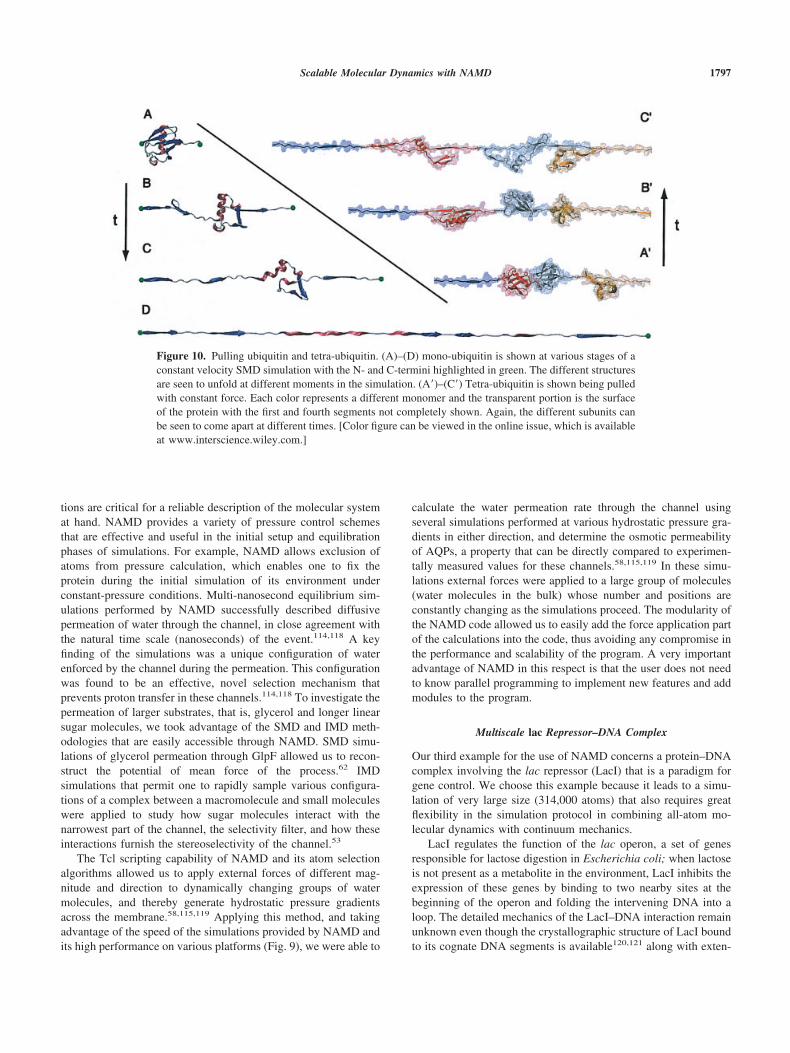
tions are critical for a reliable description of the molecular systemat hand. NAMD provides a variety of pressure control schemesthat are effective and useful in the initial setup and equilibrationphases of simulations. For example, NAMD allows exclusion ofatoms from pressure calculation, which enables one to fix theprotein during the initial simulation of its environment underconstant-pressure conditions. Multi-nanosecond equilibrium sim-ulations performed by NAMD successfully described diffusivepermeation of water through the channel, in close agreement withthe natural time scale (nanoseconds) of the event.114,118 A keyfinding of the simulations was a unique configuration of waterenforced by the channel during the permeation. This configurationwas found to be an effective, novel selection mechanism thatprevents proton transfer in these channels.114,118 To investigate thepermeation of larger substrates, that is, glycerol and longer linearsugar molecules, we took advantage of the SMD and IMD meth-odologies that are easily accessible through NAMD. SMD simu-lations of glycerol permeation through GlpF allowed us to recon-struct the potential of mean force of the process.62 IMDsimulations that permit one to rapidly sample various configura-tions of a complex between a macromolecule and small moleculeswere applied to study how sugar molecules interact with thenarrowest part of the channel, the selectivity filter, and how theseinteractions furnish the stereoselectivity of the channel.53

The Tcl scripting capability of NAMD and its atom selectionalgorithms allowed us to apply external forces of different mag-nitude and direction to dynamically changing groups of watermolecules, and thereby generate hydrostatic pressure gradientsacross the membrane.58,115,119 Applying this method, and takingadvantage of the speed of the simulations provided by NAMD andits high performance on various platforms (Fig. 9), we were able to

calculate the water permeation rate through the channel usingseveral simulations performed at various hydrostatic pressure gra-dients in either direction, and determine the osmotic permeabilityof AQPs, a property that can be directly compared to experimen-tally measured values for these channels.58,115,119 In these simu-lations external forces were applied to a large group of molecules(water molecules in the bulk) whose number and positions areconstantly changing as the simulations proceed. The modularity ofthe NAMD code allowed us to easily add the force application partof the calculations into the code, thus avoiding any compromise inthe performance and scalability of the program. A very importantadvantage of NAMD in this respect is that the user does not needto know parallel programming to implement new features and addmodules to the program.

Multiscale lac Repressor–DNA Complex

Our third example for the use of NAMD concerns a protein–DNAcomplex involving the lac repressor (LacI) that is a paradigm forgene control. We choose this example because it leads to a simu-lation of very large size (314,000 atoms) that also requires greatflexibility in the simulation protocol in combining all-atom mo-lecular dynamics with continuum mechanics.

LacI regulates the function of the lac operon, a set of genesresponsible for lactose digestion in Escherichia coli; when lactoseis not present as a metabolite in the environment, LacI inhibits theexpression of these genes by binding to two nearby sites at thebeginning of the operon and folding the intervening DNA into aloop. The detailed mechanics of the LacI–DNA interaction remainunknown even though the crystallographic structure of LacI boundto its cognate DNA segments is available120,121 along with exten-

Figure 10. Pulling ubiquitin and tetra-ubiquitin. (A)–(D) mono-ubiquitin is shown at various stages of aconstant velocity SMD simulation with the N- and C-termini highlighted in green. The different structuresare seen to unfold at different moments in the simulation. (A)–(C) Tetra-ubiquitin is shown being pulledwith constant force. Each color represents a different monomer and the transparent portion is the surfaceof the protein with the first and fourth segments not completely shown. Again, the different subunits canbe seen to come apart at different times. [Color figure can be viewed in the online issue, which is availableat www.interscience.wiley.com.]


sive biochemical and genetic data.122,123 In particular, the structurein ref. 120 does not include the DNA loop connecting the twobound DNA segments nor does it provide information on how LacIwrestles the DNA, forcing it to maintain a loop form.

A key obstacle to the simulation of the LacI–DNA dynamics isthat LacI alone is a very large protein that results, together with awater bath, in a system of 300,000 atoms; including the DNA loopwould increase the size to 700,000 atoms, thus incurring an evengreater computational cost. To overcome this difficulty one canfollow a multiscale strategy and describe the DNA loop mathe-matically employing the Kirchhoff theory of continuum elasticrods as developed in ref. 124, coupling the calculation to anall-atom MD representation of LacI. The method has been outlinedin ref. 86 and applied in ref. 6. The LacI–DNA structure con-structed in ref. 125 and employed in ref. 6 is available in theProtein Data Bank (1Z04).126 In the simulation, illustrated inFigure 12, LacI was solvated in a box of TIP3P water and 100 mMNaCl and simulated under NPT ensemble conditions with periodicboundary conditions and PME electrostatics for an overall simu-lation time of 40 ns using a 1-fs time step. At 10-ps intervals,position and orientation of the LacI head groups were communi-cated to the mathematical description of the DNA loop, which

determined the appropriate new loop geometry and communicatedback the forces and torques with which the DNA resisted theprotein’s action; forces and torques were included in the MDsimulations much like forces are incorporated in SMD runs. Sim-ulation results are shown in Figure 12. One can recognize the largescale motion of the DNA loop over the course of the simulation. Akey finding resulting from the simulation is an extreme flexibilityof the two LacI head groups absorbing most of the strain arisingfrom the DNA loop. The simulations reported in ref. 6 alsoprovided an insightful new interpretation of prior FRET data.127

NAMD proved to be most valuable due to its ability to effi-ciently simulate very large systems. In the present case NAMD rana 314,000 atom system on 256 Itanium processors of the NCSATeraGrid system with an average production speed of 2.5 ns perday. The multiscale strategy linking MD with a continuum me-chanics DNA model was implemented through the Tcl scriptinginterface of NAMD. This feature permitted us not only to obtaininformation from the simulation, for example, head group geom-etries, on the fly, but also to control from the NAMD side thecalculations for the DNA model, eventually retrieving the forcesapplied in the LacI simulation. For the sake of clarity we empha-size that the entire multiscale simulation, including the continuum

Figure 11. Side view of a simulated aquaporin tetramer in the cell membrane. The E. coli water/glycerolchannel GlpF is embedded in a patch of POPE lipid bilayer and fully hydrated by water on both sides.Lipid head groups are shown in CPK and the hydrophobic tail region is drawn using licorice represen-tation. The four AQP monomers, each forming an independent water pore, are shown in different colors.The single file of water formed inside the pores is shown in one of the monomers. The characteristicconformational inversion of water at the center of the channel that contributes to the barrier against protontransfer is discernible.


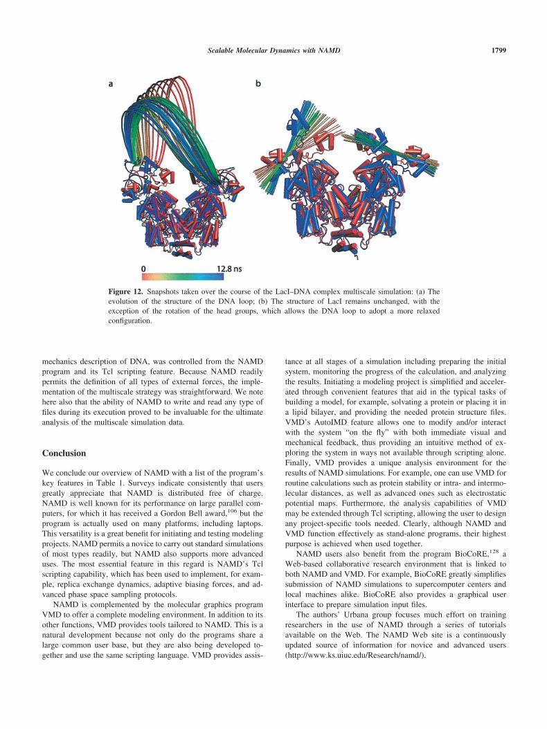
mechanics description of DNA, was controlled from the NAMDprogram and its Tcl scripting feature. Because NAMD readilypermits the definition of all types of external forces, the imple-mentation of the multiscale strategy was straightforward. We notehere also that the ability of NAMD to write and read any type offiles during its execution proved to be invaluable for the ultimateanalysis of the multiscale simulation data.

Conclusion

We conclude our overview of NAMD with a list of the program’skey features in Table 1. Surveys indicate consistently that usersgreatly appreciate that NAMD is distributed free of charge.NAMD is well known for its performance on large parallel com-puters, for which it has received a Gordon Bell award,106 but theprogram is actually used on many platforms, including laptops.This versatility is a great benefit for initiating and testing modelingprojects. NAMD permits a novice to carry out standard simulationsof most types readily, but NAMD also supports more advanceduses. The most essential feature in this regard is NAMD’s Tclscripting capability, which has been used to implement, for exam-ple, replica exchange dynamics, adaptive biasing forces, and ad-vanced phase space sampling protocols.

NAMD is complemented by the molecular graphics programVMD to offer a complete modeling environment. In addition to itsother functions, VMD provides tools tailored to NAMD. This is anatural development because not only do the programs share alarge common user base, but they are also being developed to-gether and use the same scripting language. VMD provides assis-

tance at all stages of a simulation including preparing the initialsystem, monitoring the progress of the calculation, and analyzingthe results. Initiating a modeling project is simplified and acceler-ated through convenient features that aid in the typical tasks ofbuilding a model, for example, solvating a protein or placing it ina lipid bilayer, and providing the needed protein structure files.VMD’s AutoIMD feature allows one to modify and/or interactwith the system “on the fly” with both immediate visual andmechanical feedback, thus providing an intuitive method of ex-ploring the system in ways not available through scripting alone.Finally, VMD provides a unique analysis environment for theresults of NAMD simulations. For example, one can use VMD forroutine calculations such as protein stability or intra- and intermo-lecular distances, as well as advanced ones such as electrostaticpotential maps. Furthermore, the analysis capabilities of VMDmay be extended through Tcl scripting, allowing the user to designany project-specific tools needed. Clearly, although NAMD andVMD function effectively as stand-alone programs, their highestpurpose is achieved when used together.

NAMD users also benefit from the program BioCoRE,128 aWeb-based collaborative research environment that is linked toboth NAMD and VMD. For example, BioCoRE greatly simplifiessubmission of NAMD simulations to supercomputer centers andlocal machines alike. BioCoRE also provides a graphical userinterface to prepare simulation input files.

The authors’ Urbana group focuses much effort on trainingresearchers in the use of NAMD through a series of tutorialsavailable on the Web. The NAMD Web site is a continuouslyupdated source of information for novice and advanced users(http://www.ks.uiuc.edu/Research/namd/).

Figure 12. Snapshots taken over the course of the LacI–DNA complex multiscale simulation: (a) Theevolution of the structure of the DNA loop; (b) The structure of LacI remains unchanged, with theexception of the rotation of the head groups, which allows the DNA loop to adopt a more relaxedconfiguration.


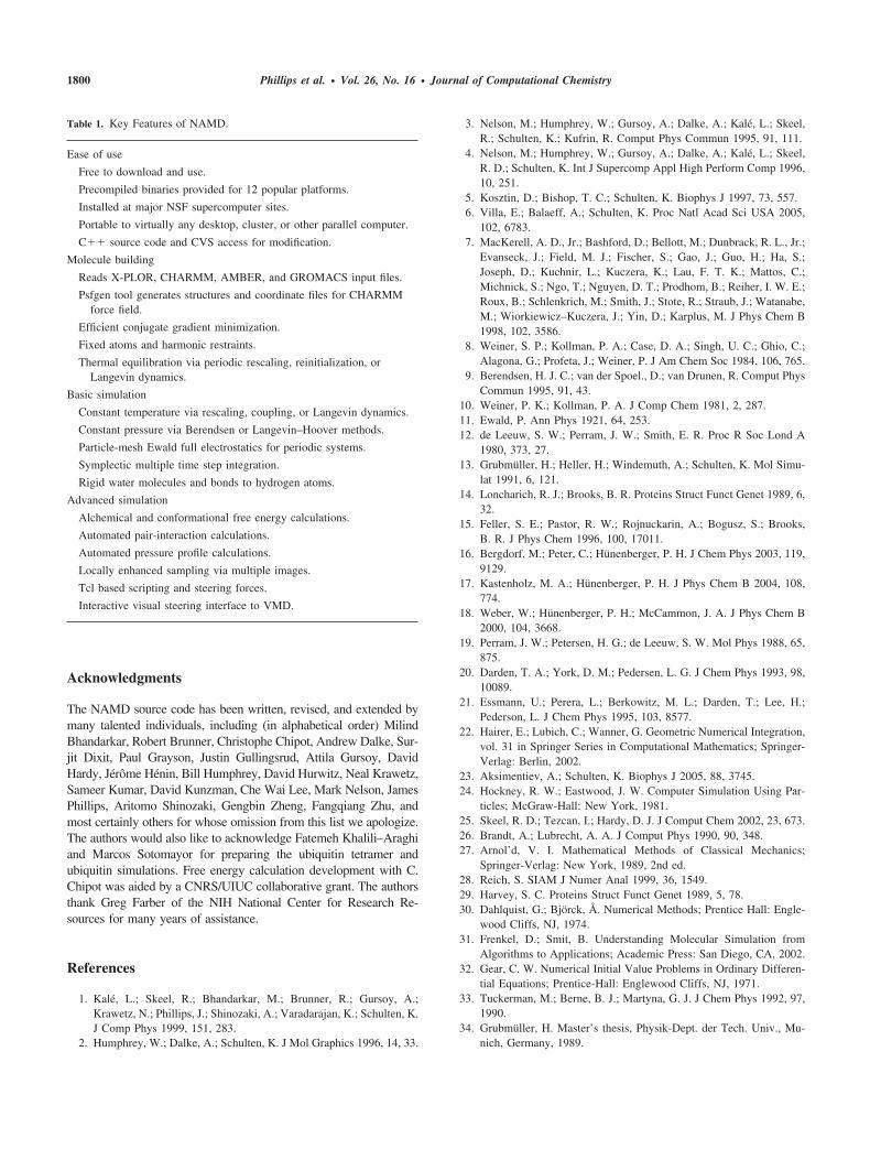
Acknowledgments

The NAMD source code has been written, revised, and extended bymany talented individuals, including (in alphabetical order) MilindBhandarkar, Robert Brunner, Christophe Chipot, Andrew Dalke, Sur-jit Dixit, Paul Grayson, Justin Gullingsrud, Attila Gursoy, DavidHardy, Jerome Henin, Bill Humphrey, David Hurwitz, Neal Krawetz,Sameer Kumar, David Kunzman, Che Wai Lee, Mark Nelson, JamesPhillips, Aritomo Shinozaki, Gengbin Zheng, Fangqiang Zhu, andmost certainly others for whose omission from this list we apologize.The authors would also like to acknowledge Fatemeh Khalili–Araghiand Marcos Sotomayor for preparing the ubiquitin tetramer andubiquitin simulations. Free energy calculation development with C.Chipot was aided by a CNRS/UIUC collaborative grant. The authorsthank Greg Farber of the NIH National Center for Research Re-sources for many years of assistance.

References

1. Kale, L.; Skeel, R.; Bhandarkar, M.; Brunner, R.; Gursoy, A.;Krawetz, N.; Phillips, J.; Shinozaki, A.; Varadarajan, K.; Schulten, K.J Comp Phys 1999, 151, 283.

2. Humphrey, W.; Dalke, A.; Schulten, K. J Mol Graphics 1996, 14, 33.

3. Nelson, M.; Humphrey, W.; Gursoy, A.; Dalke, A.; Kale, L.; Skeel,R.; Schulten, K.; Kufrin, R. Comput Phys Commun 1995, 91, 111.

4. Nelson, M.; Humphrey, W.; Gursoy, A.; Dalke, A.; Kale, L.; Skeel,R. D.; Schulten, K. Int J Supercomp Appl High Perform Comp 1996,10, 251.

5. Kosztin, D.; Bishop, T. C.; Schulten, K. Biophys J 1997, 73, 557.6. Villa, E.; Balaeff, A.; Schulten, K. Proc Natl Acad Sci USA 2005,

102, 6783.7. MacKerell, A. D., Jr.; Bashford, D.; Bellott, M.; Dunbrack, R. L., Jr.;

Evanseck, J.; Field, M. J.; Fischer, S.; Gao, J.; Guo, H.; Ha, S.;Joseph, D.; Kuchnir, L.; Kuczera, K.; Lau, F. T. K.; Mattos, C.;Michnick, S.; Ngo, T.; Nguyen, D. T.; Prodhom, B.; Reiher, I. W. E.;Roux, B.; Schlenkrich, M.; Smith, J.; Stote, R.; Straub, J.; Watanabe,M.; Wiorkiewicz–Kuczera, J.; Yin, D.; Karplus, M. J Phys Chem B1998, 102, 3586.

8. Weiner, S. P.; Kollman, P. A.; Case, D. A.; Singh, U. C.; Ghio, C.;Alagona, G.; Profeta, J.; Weiner, P. J Am Chem Soc 1984, 106, 765.

9. Berendsen, H. J. C.; van der Spoel., D.; van Drunen, R. Comput PhysCommun 1995, 91, 43.

10. Weiner, P. K.; Kollman, P. A. J Comp Chem 1981, 2, 287.11. Ewald, P. Ann Phys 1921, 64, 253.12. de Leeuw, S. W.; Perram, J. W.; Smith, E. R. Proc R Soc Lond A

1980, 373, 27.13. Grubmuller, H.; Heller, H.; Windemuth, A.; Schulten, K. Mol Simu-

lat 1991, 6, 121.14. Loncharich, R. J.; Brooks, B. R. Proteins Struct Funct Genet 1989, 6,

32.15. Feller, S. E.; Pastor, R. W.; Rojnuckarin, A.; Bogusz, S.; Brooks,

B. R. J Phys Chem 1996, 100, 17011.16. Bergdorf, M.; Peter, C.; Hunenberger, P. H. J Chem Phys 2003, 119,

9129.17. Kastenholz, M. A.; Hunenberger, P. H. J Phys Chem B 2004, 108,

774.18. Weber, W.; Hunenberger, P. H.; McCammon, J. A. J Phys Chem B

2000, 104, 3668.19. Perram, J. W.; Petersen, H. G.; de Leeuw, S. W. Mol Phys 1988, 65,

875.20. Darden, T. A.; York, D. M.; Pedersen, L. G. J Chem Phys 1993, 98,

10089.21. Essmann, U.; Perera, L.; Berkowitz, M. L.; Darden, T.; Lee, H.;

Pederson, L. J Chem Phys 1995, 103, 8577.22. Hairer, E.; Lubich, C.; Wanner, G. Geometric Numerical Integration,

vol. 31 in Springer Series in Computational Mathematics; Springer-Verlag: Berlin, 2002.

23. Aksimentiev, A.; Schulten, K. Biophys J 2005, 88, 3745.24. Hockney, R. W.; Eastwood, J. W. Computer Simulation Using Par-

ticles; McGraw-Hall: New York, 1981.25. Skeel, R. D.; Tezcan, I.; Hardy, D. J. J Comput Chem 2002, 23, 673.26. Brandt, A.; Lubrecht, A. A. J Comput Phys 1990, 90, 348.27. Arnol’d, V. I. Mathematical Methods of Classical Mechanics;

Springer-Verlag: New York, 1989, 2nd ed.28. Reich, S. SIAM J Numer Anal 1999, 36, 1549.29. Harvey, S. C. Proteins Struct Funct Genet 1989, 5, 78.30. Dahlquist, G.; Bjorck, Å. Numerical Methods; Prentice Hall: Engle-

wood Cliffs, NJ, 1974.31. Frenkel, D.; Smit, B. Understanding Molecular Simulation from

Algorithms to Applications; Academic Press: San Diego, CA, 2002.32. Gear, C. W. Numerical Initial Value Problems in Ordinary Differen-

tial Equations; Prentice-Hall: Englewood Cliffs, NJ, 1971.33. Tuckerman, M.; Berne, B. J.; Martyna, G. J. J Chem Phys 1992, 97,

1990.34. Grubmuller, H. Master’s thesis, Physik-Dept. der Tech. Univ., Mu-

nich, Germany, 1989.

Table 1. Key Features of NAMD.

Ease of use

Free to download and use.

Precompiled binaries provided for 12 popular platforms.

Installed at major NSF supercomputer sites.

Portable to virtually any desktop, cluster, or other parallel computer.

C�� source code and CVS access for modification.

Molecule building

Reads X-PLOR, CHARMM, AMBER, and GROMACS input files.

Psfgen tool generates structures and coordinate files for CHARMMforce field.

Efficient conjugate gradient minimization.

Fixed atoms and harmonic restraints.

Thermal equilibration via periodic rescaling, reinitialization, orLangevin dynamics.

Basic simulation

Constant temperature via rescaling, coupling, or Langevin dynamics.

Constant pressure via Berendsen or Langevin–Hoover methods.

Particle-mesh Ewald full electrostatics for periodic systems.

Symplectic multiple time step integration.

Rigid water molecules and bonds to hydrogen atoms.

Advanced simulation

Alchemical and conformational free energy calculations.

Automated pair-interaction calculations.

Automated pressure profile calculations.

Locally enhanced sampling via multiple images.

Tcl based scripting and steering forces.

Interactive visual steering interface to VMD.


35. Bishop, T. C.; Skeel, R. D.; Schulten, K. J Comp Chem 1997, 18, 1785.36. Ma, Q.; Izaguirre, J. A.; Skeel, R. D. SIAM J Sci Comput 2003, 24,

1951.37. Kubo, R.; Toda, M.; Hashitsume, N. Statistical Physics II: Nonequi-

librium Statistical Mechanics; Springer: New York, 1991, 2nd ed.38. Brunger, A.; Brooks, C. B.; Karplus, M. Chem Phys Lett 1984, 105,

495.39. Mishra, B.; Schlick, T. J Chem Phys 1996, 105, 299.40. Wang, W.; Skeel, R. D. Mol Phys 2003, 101, 2149.41. Park, S.; Schulten, K. J Chem Phys 2004, 120, 5946.42. Tuckerman, M.; Liu, Y.; Ciccotti, G.; Martyna, G. J. J Chem Phys

2001, 115, 1678.43. Bhandarkar, M.; Brunner, R.; Chipot, C.; Dalke, A.; Dixit, S.; Gray-

son, P.; Gullingsrud, J.; Gursoy, A.; Hardy, D.; Humphrey, W.;Hurwitz, D.; Krawetz, N.; Nelson, M.; Phillips, J.; Shinozaki, A.;Zheng, G.; Zhu, F. NAMD user’s guide version 2.5. http://www.ks.uiuc.edu/Research/namd/2.5/ug/ug.html.

44. Feller, S. E.; Zhang, Y.; Pastor, R. W.; Brooks, B. R. J Chem Phys1995, 103, 4613.

45. Hoover, W. G. Phys Rev A 1985, 31, 1695.46. Hoover, W. G. Phys Rev A 1986, 34, 2499.47. Hoover, W. G. Computational Statistical Mechanics; Elsevier: Am-

sterdam, 1991.48. Quigley, D.; Probert, M. I. J. J Chem Phys 2004, 120, 11432.49. Izrailev, S.; Stepaniants, S.; Isralewitz, B.; Kosztin, D.; Lu, H.;

Molnar, F.; Wriggers, W.; Schulten, K. Computational MolecularDynamics: Challenges, Methods, Ideas, vol. 4 in Lecture Notes inComputational Science and Engineering; Deuflhard, P.; Hermans, J.;Leimkuhler, B.; Mark, A. E.; Reich, S.; Skeel, R. D., Eds.; Springer-Verlag: Berlin, 1998, p. 39.

50. Isralewitz, B.; Baudry, J.; Gullingsrud, J.; Kosztin, D.; Schulten, K.J Mol Graph Model 2001, 19, 13; Also in Protein Flexibility andFolding, Kuhn, L. A.; Thorpe, M. F., Eds.; Elsevier: New York.

51. Isralewitz, B.; Gao, M.; Schulten, K. Curr Opin Struct Biol 2001, 11,224.

52. Stone, J.; Gullingsrud, J.; Grayson, P.; Schulten, K. In 2001 ACMSymposium on Interactive 3D Graphics; Hughes, J. F.; Sequin, C. H.,Eds.; ACM SIGGRAPH: New York, 2001, p. 191.

53. Grayson, P.; Tajkhorshid, E.; Schulten, K. Biophys J 2003, 85, 36.54. Gullingsrud, J.; Braun, R.; Schulten, K. J Comp Phys 1999, 151, 190.55. Sotomayor, M.; Corey, D. P.; Schulten, K. Structure 2005, 13, 669.56. Craig, D.; Gao, M.; Schulten, K.; Vogel, V. Structure 2004, 12, 2049.57. Aksimentiev, A.; Balabin, I. A.; Fillingame, R. H.; Schulten, K.

Biophys J 2004, 86, 1332.58. Zhu, F.; Tajkhorshid, E.; Schulten, K. Biophys J 2004, 86, 50.59. Gullingsrud, J.; Schulten, K. Biophys J 2003, 85, 2087.60. Bayas, M. V.; Schulten, K.; Leckband, D. Biophys J 2003, 84, 2223.61. Gao, M.; Wilmanns, M.; Schulten, K. Biophys J 2002, 83, 3435.62. Jensen, M. Ø.; Park, S.; Tajkhorshid, E.; Schulten, K. Proc Natl Acad

Sci USA 2002, 99, 6731.63. Kosztin, D.; Izrailev, S.; Schulten, K. Biophys J 1999, 76, 188.64. Lu, H.; Schulten, K. Proteins Struct Funct Genet 1999, 35, 453.65. Stepaniants, S.; Izrailev, S.; Schulten, K. J Mol Mod 1997, 3, 473.66. Izrailev, S.; Crofts, A. R.; Berry, E. A.; Schulten, K. Biophys J 1999,

77, 1753.67. Izrailev, S.; Stepaniants, S.; Balsera, M.; Oono, Y.; Schulten, K.

Biophys J 1997, 72, 1568.68. Isralewitz, B.; Izrailev, S.; Schulten, K. Biophys J 1997, 73, 2972.69. Grubmuller, H.; Heymann, B.; Tavan, P. Science 1996, 271, 997.70. Kosztin, D.; Izrailev, S.; Schulten, K. Biophys J 1999, 76, 188.71. Torrie, G. M.; Valleau, J. P. J Comput Phys 1977, 23, 187.72. Roux, B. Comput Phys Commun 1995, 91, 275.73. Schulten, K.; Schulten, Z.; Szabo, A. J Chem Phys 1981, 74, 4426.

74. Lu, H.; Krammer, A.; Isralewitz, B.; Vogel, V.; Schulten, K. InElastic Filaments of the Cell; Pollack, J.; Granzier, H., Eds.; KluwerAcademic/Plenum Publishers: New York, 2000, p. 143, chap 1.

75. Lu, H.; Schulten, K. Biophys J 2000, 79, 51.76. Jarzynski, C. Phys Rev Lett 1997, 78, 2690.77. Jarzynski, C. Phys Rev E 1997, 56, 5018.78. Liphardt, J.; Dumont, S.; Smith, S.; Tinoco, I.; Bustamante, C.

Science 2002, 296, 1832.79. Hummer, G.; Rasaiah, J. C.; Noworyta, J. P. Nature 2001, 414, 188.80. Marcinkiewicz, J. Math Z 1939, 44, 612.81. Park, S.; Khalili-Araghi, F.; Tajkhorshid, E.; Schulten, K. J Chem

Phys 2003, 119, 3559.82. Kumar, S.; Bouzida, D.; Swendsen, R. H.; Kollman, P. A.; Rosen-

berg, J. M. J Comp Chem 1992, 13, 1011.83. Boczko, E. M.; Brooks, C. L., III. J Phys Chem 1993, 97, 4509.84. Shea, J. E.; Brooks, C. L., III. Annu Rev Phys Chem 2001, 52, 499.85. Aksimentiev, A.; Balabin, I. A.; Fillingame, R. H.; Schulten, K.

Biophys J 2004, 86, 1332.86. Villa, E.; Balaeff, A.; Mahadevan, L.; Schulten, K. Multiscale Model

Simul 2004, 2, 527.87. Taylor, R. M., II. VRPN: Virtual Reality Peripheral Network, 1998.

http://www.cs.unc.edu/Research/vrpn.88. Dachille, F.; Qin, H.; Kaufman, A.; El-Sana, J. In 1999 Symposium

on Interactive 3D Graphics, 1999, p. 103.89. Cohen, J.; Grayson, P. AutoIMD User’s Guide, 2003. http://www.

ks.uiuc.edu/Research/vmd/plugins/autoimd.90. den Otter, W. K.; Briels, W. J. J Chem Phys 1998, 109, 4139.91. Zwanzig, R. W. J Chem Phys 1954, 22, 1420.92. Darve, E.; Pohorille, A. J Chem Phys 2001, 115, 9169.93. Henin, J.; Chipot, C. J Chem Phys 2004, 121, 2904.94. Gao, J.; Kuczera, K.; Tidor, B.; Karplus, M. Science 1989, 244, 1069.95. Fleming, K. G.; Ackerman, A. L.; Engelman, D. M. J Mol Biol 1997,

272, 266.96. Henin, J.; Pohorille, A.; Chipot, C. J Am Chem Soc 2005, 127, 8478.97. Allen, M. P.; Tildesley, D. J. Computer Simulation of Liquids;

Oxford University Press: New York, 1987.98. Kale, L. V.; Krishnan, S. Parallel Programming using C��; Wilson,

G. V.; Lu, P., Eds.; MIT Press: Cambridge, MA, 1996, p. 175.99. Kale, L. V. In LACSI 2002; Albuquerque, 2002.

100. Brunner, R. K.; Kale, L. V. In Parallel and Distributed Computing forSymbolic and Irregular Applications; World Scientific Publishing:Singapore, 2000, p. 167.

101. Phillips, J. C.; Brunner, R.; Shinozaki, A.; Bhandarkar, M.; Krawetz,N.; Kale, L.; Skeel, R. D.; Schulten, K. In Computational MolecularDynamics: Challenges, Methods, Ideas; vol. 4 in Lecture Notes inComputational Science and Engineering; Deuflhard, P.; Hermans, J.;Leimkuhler, B.; Mark, A.; Reich, S.; Skeel, R. D., Eds.; Springer-Verlag: Berlin, 1998, p. 472.

102. Ousterhout, J. Tcl and the Tk Toolkit; Addison-Wesley: Reading,MA; 1994.

103. Sugita, Y.; Okamoto, Y. Chem Phys Lett 1999, 314, 141.104. Kale, L. V.; Zheng, G.; Lee, C. W.; Kumar, S. In Future Generation

Computer Systems Special Issue on: Large-Scale System Perfor-mance Modeling and Analysis; in press.

105. Petrini, F.; Kerbyson, D. J.; Pakin, S. In Proceedings of the IEEE/ACMSC2003 Conference, Technical Paper 301; IEEE Press: Piscataway, NJ,2003.

106. Phillips, J.; Zheng, G.; Kumar, S.; Kale, L. In Proceedings of theIEEE/ACM SC2002 Conference, Technical Paper 277; IEEE Press:Piscataway, NJ, 2002.

107. Hershko, A.; Heller, H.; Elias, S.; Ciechanover, A. J Biol Chem 1983,258, 8206.

108. Haas, A. L.; Rose, I. A. J Biol Chem 1982, 257, 10329.


109. Hershko, A.; Ciechanover, A. Annu Rev Biochem 1998, 67, 425.110. Carrion–Vazquez, M.; Li, H.; Lu, H.; Marszalek, P. E.; Oberhauser,

A. F.; Fernandez, J. M. Nat Struct Biol 2003, 10, 738.111. Fernandez, J. M.; Li, H. Science 2004, 303, 1674.112. Zhu, F.; Tajkhorshid, E.; Schulten, K. FEBS Lett 2001, 504, 212.113. Jensen, M. Ø; Tajkhorshid, E.; Schulten, K. Structure 2001, 9,

1083.114. Tajkhorshid, E.; Nollert, P.; Jensen, M. Ø; Miercke, L. J. W.;

O’Connell, J.; Stroud, R. M.; Schulten, K. Science 2002, 296, 525.115. Zhu, F.; Tajkhorshid, E.; Schulten, K. Biophys J 2002, 83, 154.116. Roux, B.; Schulten, K. Structure 2004, 12, 1343.117. Tajkhorshid, E.; Cohen, J.; Aksimentiev, A.; Sotomayor, M.; Schulten,

K. In Bacterial Ion Channels and Their Eukaryotic Homologues; Mar-tinac, B.; Kubalski, A., Eds.; ASM Press: Washington, DC, 2005, p. 153.

118. Jensen, M. Ø; Tajkhorshid, E.; Schulten, K. Biophys J 2003, 85,2884.

119. Zhu, F.; Tajkhorshid, E.; Schulten, K. Phys Rev Lett 2004, 93,224501.

120. Lewis, M.; Chang, G.; Horton, N. C.; Kercher, M. A.; Pace, H. C.;Schumacher, M. A.; Brennan, R. G.; Lu, P. Science 1996, 271, 1247.

121. Friedman, A. M.; Fischmann, T. O.; Steitz, T. A. Science 1995, 268,1721.

122. Ptashne, M. A Genetic Switch; Cell Press & Blackwell ScientificPublications: Cambridge, MA, 1992, 2nd ed.

123. Muller–Hill, B. The lac Operon; Walter de Gruyter: New York, 1996.124. Balaeff, A.; Koudella, C. R.; Mahadevan, L.; Schulten, K. Philos

Trans R Soc Lond A 2004, 362, 1355.125. Balaeff, A.; Mahadevan, L.; Schulten, K. Structure 2004, 12, 123.126. The RCSB Protein Data Bank. http://www.rcsb.org/pdb.127. Edelman, L. M.; Cheong, R.; Kahn, J. D. Biophys J 2003, 84, 1131.128. Bhandarkar, M.; Budescu, G.; Humphrey, W.; Izaguirre, J. A.; Izrai-

lev, S.; Kale, L. V.; Kosztin, D.; Molnar, F.; Phillips, J. C.; Schulten,K. In Proceedings of the SCS International Conference on Web-Based Modeling and Simulation; Bruzzone, A. G.; Uchrmacher, A.;Page, E. H., Eds.; SCS International, San Francisco: San Francisco,CA, 1999, p. 242.


Documents

Scalable Molecular Dynamics with NAMD - Virginia …people.cs.vt.edu/npolys/IT/VMD-NAMD.pdf · Scalable Molecular Dynamics with NAMD ... alchemical and conformational free energy