SBGf 2015 Denise

7/23/2019 SBGf 2015 Denise

http://slidepdf.com/reader/full/sbgf-2015-denise 1/6

Fourteenth International Congress of the Brazilian Geophysical Society

Magnetic study of Saint Paul Fracture Zone, Equatorial AtlanticDenise S. Moura* (IAG/USP), Márcia Maia (CNRS-IUEM/UBO), Yára R. Marangoni (IAG/USP), Susanna E. Sichel(LAGEMAR, UFF) and Ivo Pessanha (CPRM)

Copyright 2015, SBGf - Sociedade Brasileira de Geofísica

This paper was prepared for presentation during the 14 th International Congress of theBrazilian Geophysical Society held in Rio de Janeiro, Brazil, August 3-6, 2015.

Contents of this paper were reviewed by the Technical Committee of the 14 th International Congress of the Brazilian Geophysical Society and do not necessarilyrepresent any position of the SBGf, its officers or members. Electronic reproduction orstorage of any part of this paper for commercial purposes without the written consentof the Brazilian Geophysical Society is prohibited. ____________________________________________________________________

Abstract

The magnetic study of Saint Paul fracture zone is partof the COLMEIA Project (Cold Mantle Exhumation andIntra-transform Accretion), and deals with themagnetic data collected during the oceanographiccruise on January-February of 2013. Firstly, the datawas processed and the initial analysis was done,getting an observed magnetic anomalies grid. Thesecond focus was the calculation of simpletheoretical models able to simulate an homogeneouscrust with constant spreading, and topography andtwo magnetization possibilities: a constant value or afunction of age. Therefore, the processed modelsrepresent a simple dynamic. The residuals, i.e., thedifferences between the observed and theoreticalsignal, show variations in composition, topographyand polarity. Differences between models will bepresented and discussed. The interpretation of theresidual anomalies, compared with other geophysical

and geological data, will be able to partially model thegeodynamical processes in the region, specifically inthe area of St. Paul’s fracture and the St. Peter and St.Paul’s Archipelago. The interpretation had alreadystarted and this work aims to present the first ideasfrom the magnetic analysis of COLMEIA cruise.

Introduction

In 2013 the international project COLMEIA begun thestudy of St. Paul Fracture Zone through anoceanographic cruise where geologic, geophysics, andchemistry data were collected. In this extend abstract theinitial analysis of the magnetic data is presented.

One of the main objects in geophysical studies in theoceanic crust is the magnetostratigraphy: The challengeof determining the ocean floor age based on magneticanomalies. The magnetic rocks that form the ocean floorguarantee the record of geomagnetic field while they cooldown, resulting in a linear anomaly pattern parallel to theridge. However, the typical magnetic profiles, like thoseobserved in Vine and Matthews (1963), were notidentifiable at the study area due to the very low magneticlatitude, which compromises the amplitude of the normaland reversely anomalies.

The technique of reduction to the pole is used as a tool toenhance the signal for magnetic surveys at low latitudes(Hansen and Pawlowski, 1989; Luo and Xue, 2009). Inspite of that, this work uses another approach, theforward modeling. It was adapted from a study publishedby Maia et al. (2005) which presents a magnetic modelingof oceanic crust in South Pacific as an independent meanof dating volcanic edifices.

This work proposes three magnetic computed modelswith a simple dynamic behind them. The parameters werechosen carefully, avoiding a complex model, so aninterpretation of the differences between the models and

the observed magnetic anomaly grid could be done.Materials and Methods

Available data The observed data consists in multibeambathymetry (Maia et al., 2013) and surface magneticmeasurements each 10 seconds. The bathymetric gridcan be seen in Figure 1 and the magnetic anomalies inFigure 2. IGRF-11 was removed from the Total MagneticField for each point.

The ship tracks are mostly oriented EW and NS. Usually,profiles in the spreading direction (EW) are better for theidentification of the magnetic anomalies and dating theoceanic crust, while perpendicular seismic arrays (NS)identify more precisely transform fault related structures

and the fracture zone.The minimum distance between the ship and themagnetometer was enough to avoid magnetic influence ofthe ship metallic mass. The measurements are made withan Overhauser magnetometer with 0.001nT resolutionand 0.1nT absolute accuracy. A low-pass filtering and aspike-sorting algorithm were applied to removeacquisition errors from the database. The early dataprocessing and validation was done on board.

An important correction for magnetic land surveys is thediurnal variation. It is not done on offshore campaigns dueto the need of keep a static magnetometer near the area,which is obviously not possible. However, the amplitudeof diurnal variation is smaller in marine surveys (Jones,

1999) ensuring the data validation. In the oceans,electromagnetic induction tends to reduce diurnalvariation amplitude, but it is a variable phenomenon. Flowof electrically conducting seawater produces fieldchanges that depend upon the speed and the direction ofthe water movement with respect to the magnetic polesand the conductivity structure of the seabed. Recordingsfrom the nearest land magnetic observatory cannot beused to take account of offshore diurnal variation withoutthe risk of large amplitude errors (Parkinson and Jones,1979; Hill and Mason, 1962). This condition made the useof Brazil and Africa’s observatories impracticable.

7/23/2019 SBGf 2015 Denise


M AGNETIC STUDY OF ST. P AUL FRACTURE ZONE ________________________________________________________________________________________________________________________________________________________________________________________________________________________________________________________________________________________________________________________________________________________________________________________________________________________________________________________________________________


2

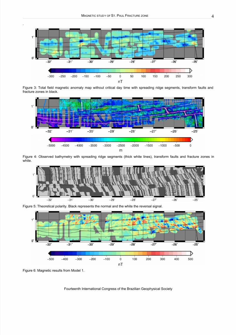
In practice, an analysis of diurnal variation is made todetermine if the critical interval, between 10 a.m. and 3p.m., define differences with other days’ time. If this hasoccurred the only solution would be to remove thosepoints. Fortunately, comparing the complete grid and thegrid without critical time (Figure 3) only few differenceswere found. This study used all data to make themagnetic survey grid and thus follows the currentprocedures for processing of marine magnetic data.

After all corrections and analysis, the observed databaseresulted in accurate anomalies.

Model assumptions This work assumed that magneticanomalies are dominated by thermoremanentmagnetization (TRM). By theoretical magnetic studies, itis known that very dynamic areas with hydrothermalcirculation have a remagnetization at most of one third ofthe natural remanent magnetization (NRM) (Hall et al.,1995). This is due to the magnetic moment of the grain,the dependence of time, related to the size and thetemperature. The thermal energy decreases the basaltmagnetization exponentially. This is guided by thefundamental process called maghemitization, which

consists in the transformation of titanomagnetite totitanomaghemite. For moderate oxidation of singledomain size grains, the chemical remanent magnetization(CRM) direction, related to maghemitization on this case,is the same as that of the TRM, so that magnetic stripeanomalies should be unchanged in terms ofmagnetization direction, only the amplitude will change(Dunlop and Özdemir, 1997). This is the affirmation thatvalidates Vine and Matthews’s theory for the presentstudy.

The magnetization model’s constant parameters are:

- A layer of 500 m thickness that supports thehypothesis of a young crust, recently magnetized(Ade-Hall et al., 1975).

- Five spreading ridges, including two segments partsof the Mid-Atlantic ridge and three intra-transformsegments. They have been delimited by theircharacteristic morphology (Figure 4).

- A constant spreading rate along each segment, theirdirections were calculated using a set of rotationpoles for South America and Africa plates.

- A homogeneous crust of tholeiitic basalt.

The flowlines were calculated as a function of time, so anage grid was interpolated and defined isochrones everymillion year. The age at the center of each ridge segment,at the neo-volcanic ridge, is zero. In the Figure 4 it is

presented the trace of the active transform faults and thecorresponding inactive fracture zones traced visuallyfollowing the valleys structures roughly parallel to thespreading direction.

The second constructed grid contained the expectedmagnetic polarities ascribed depending on the age. Thepolarity time scale uses the range of 35 Ma defined byCande and Kent (1995). A grid with this information wasset and is shown in Figure 5. It indicates the normal and

reversal signals of each age strip. The modeling aims tosimulate this influence on the magnetic signal.

Models This work compares three models. Thedistinctions among them are in the Table 1. They werecalculated with a project algorithm, an adaptation on thealgorithm of Maia et al. (2005), which combine the age,the magnetic polarity and the ocean floor depth grids tocalculate the magnetic anomalies formed by the TRM of

the oceanic crust.Table1: Models constructed for this study.

1 2 3

Magnetization Equation 1 Equation 1 10 [A/m]

Topography Observed Equation 2 Equation 2

(1)

(2)

Models 1 and 2 consider a decrease of magnetization asa function of age, equation (1). The initial value 10 A/m isan estimative of the magnetization of a zero age basaltcrust. Model 3 assumes a constant magnetization equalto the initial value. The dependence of time is aconsequence of viscous and chemical remanentmagnetizations, as discussed earlier in the modelassumptions. The parameter 2.1737 follows the sameempirical relation used in Maia et al. (2005).

The first model used the observed bathymetry and theothers a depth dependent of time (equation 2). The depthincreases with age as the oceanic lithosphere subsides.This particular relation was presented by Parsons andSclater (1977). The minridge is the value of minimumtopography at the ridge axis. It was set as 2500 m for theNorth and South segments, 3000 m for the intra-transformNorth segment and 3200 m for the central and south

segments. These values had been chosen visually fromthe bathymetry map, Figure 4.

Results and Preliminary Conclusions

The three models represent different possibilities to themagnetic anomalies related to a simple spreading modelfor the area of the St. Paul fracture zone.

Model 1 (Figure 6) presents high amplitude anomaliesaround the accretion axes and an approximately paralleldistribution of the polarities. The anomalies induced bythe boundaries between plates with different polarity andages are noticeable. Besides, the model does notsystematically present a mirror effect between the twoflanks of the ridge.

Model 2 (Figure 7) shows magnetic anomalies with smallamplitudes. The symmetry between the two flanks of theridges is not very clear, either.

Comparing models 1 and 2 it is possible to noticesignificant differences. The observed bathymetry (model1) presents higher anomaly amplitudes and they aredistributed in a larger area. Since the models differ only inthe bathymetric input (Table 1) it is possible to associatethe differences to the effect of the topography, which is

7/23/2019 SBGf 2015 Denise


MOURA, M AIA & M ARANGONI ________________________________________________________________________________________________________________________________________________________________________________________________________________________________________________________________________________________________________________________________________________________________________________________________________________________________________________________________________________


3

very pronounced in the study area and not always directlyrelated to the normal spreading process.

Model 3 (Figure 8) was formulated to evaluate the effectof the attenuation of the magnetization with time in atheoretical model.

The amplitude anomalies and the alignment of them inmodel 3 related to the observed anomalies (Figure 2) mayalert that the calculated decay may be stronger than theobserved in equatorial region. Therefore, a specific modelfor magnetic decay at equatorial region must be set.

The residual anomalies are the difference between thecalculated and the observed grid. Models 1 and 2 wereused to calculate the residual anomalies. Results arepresented in figures 9, 10 and 11, they show thedifference between the calculated magnetic grid (Figures6 and 7) and the observed anomaly grid (Figure 2).

The residual grid for the model 1 revealed an interestingpoint:

- The higher anomalies close to the accretionregion (Figure 9). It could be explained by thesame magnetization decay considered in thisstudy, although, the first million years has fastervariations. It is known that the fine grains inquenched pillows, in contact with seawater andwarmed through burial beneath later eruptions,

oxidize rapidly, certainly within 0.5 Ma (Irving,1970; Ozima, 1971; Johnson and Atwater, 1977and Johnson and Pariso, 1993).

The residual for model 2 has very similar anomaliescomparing to the residual for model 1, since this models just differs in the input topography. The followingcharacteristics revealed are:

- The negative anomaly caused by St. Peter andSt. Paul Archipelago, 29.5°W, and the St. Paultransform fault (Figure 10). It was expected dueto the low magnetization from mantle andmetamorphic rocks collected during the cruisecompared to the tholeiitic basalt used in themodels.

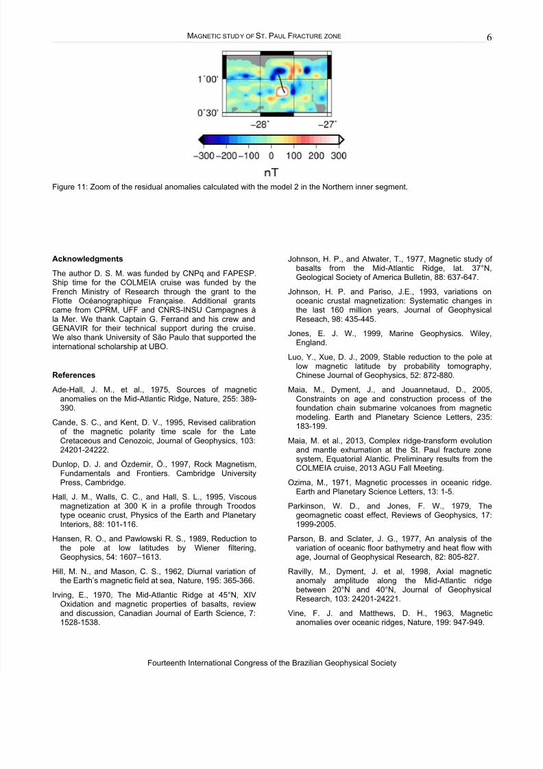
- The alteration action on the axes, easilyidentifiable on the intra-transform segments, asin 27.7°W, this axis has a negative anomalyassociated with its north part and a very positiveanomaly associated with its south part (Figure11). A theoretical explanation is that “Shallowfractionation and serpentinization of ultramaficrocks at segment ends control the amplitude

variation within segments. The balance betweenthese processes depends on the thermal stateamong segments” (Ravilly and Dyment, 1998).

Figures

Figure 1: Multibeam bathymetry with track profiles.

Figure 2: Total field magnetic anomaly map with spreading ridge segments, transform faults and fracture zones in black.

7/23/2019 SBGf 2015 Denise




4

.

Figure 3: Total field magnetic anomaly map without critical day time with spreading ridge segments, transform faults andfracture zones in black.

Figure 4: Observed bathymetry with spreading ridge segments (thick white lines), transform faults and fracture zones inwhite.

Figure 5: Theoretical polarity. Black represents the normal and the white the reversal signal.

Figure 6: Magnetic results from Model 1.

7/23/2019 SBGf 2015 Denise


MOURA, M AIA & M ARANGONI ________________________________________________________________________________________________________________________________________________________________________________________________________________________________________________________________________________________________________________________________________________________________________________________________________________________________________________________________________________


5



Figure 9: Zoom of the residual anomalies calculated with the model 1 in the Northern Mid-Ocean ridge.

Figure 10: Zoom of the residual anomalies calculated with the model 2 in the St. Paul fracture zone. The linear negativeanomaly of the fracture zone is delimited.

7/23/2019 SBGf 2015 Denise




6

Figure 11: Zoom of the residual anomalies calculated with the model 2 in the Northern inner segment.

Acknowledgments

The author D. S. M. was funded by CNPq and FAPESP.Ship time for the COLMEIA cruise was funded by theFrench Ministry of Research through the grant to theFlotte Océanographique Française. Additional grantscame from CPRM, UFF and CNRS-INSU Campagnes àla Mer. We thank Captain G. Ferrand and his crew andGENAVIR for their technical support during the cruise.We also thank University of São Paulo that supported theinternational scholarship at UBO.

References

Ade-Hall, J. M., et al., 1975, Sources of magneticanomalies on the Mid-Atlantic Ridge, Nature, 255: 389-390.

Cande, S. C., and Kent, D. V., 1995, Revised calibrationof the magnetic polarity time scale for the LateCretaceous and Cenozoic, Journal of Geophysics, 103:24201-24222.

Dunlop, D. J. and Özdemir, Ö., 1997, Rock Magnetism,Fundamentals and Frontiers. Cambridge UniversityPress, Cambridge.

Hall, J. M., Walls, C. C., and Hall, S. L., 1995, Viscousmagnetization at 300 K in a profile through Troodostype oceanic crust, Physics of the Earth and PlanetaryInteriors, 88: 101-116.

Hansen, R. O., and Pawlowski R. S., 1989, Reduction tothe pole at low latitudes by Wiener filtering,Geophysics, 54: 1607 –1613.

Hill, M. N., and Mason, C. S., 1962, Diurnal variation ofthe Earth’s magnetic field at sea, Nature, 195: 365-366.

Irving, E., 1970, The Mid-Atlantic Ridge at 45°N, XIVOxidation and magnetic properties of basalts, reviewand discussion, Canadian Journal of Earth Science, 7:1528-1538.

Johnson, H. P., and Atwater, T., 1977, Magnetic study of

basalts from the Mid-Atlantic Ridge, lat. 37°N,Geological Society of America Bulletin, 88: 637-647.

Johnson, H. P. and Pariso, J.E., 1993, variations onoceanic crustal magnetization: Systematic changes inthe last 160 million years, Journal of GeophysicalReseach, 98: 435-445.

Jones, E. J. W., 1999, Marine Geophysics. Wiley,England.

Luo, Y., Xue, D. J., 2009, Stable reduction to the pole atlow magnetic latitude by probability tomography,Chinese Journal of Geophysics, 52: 872-880.

Maia, M., Dyment, J., and Jouannetaud, D., 2005,Constraints on age and construction process of thefoundation chain submarine volcanoes from magneticmodeling. Earth and Planetary Science Letters, 235:183-199.

Maia, M. et al., 2013, Complex ridge-transform evolutionand mantle exhumation at the St. Paul fracture zonesystem, Equatorial Alantic. Preliminary results from theCOLMEIA cruise, 2013 AGU Fall Meeting.

Ozima, M., 1971, Magnetic processes in oceanic ridge.Earth and Planetary Science Letters, 13: 1-5.

Parkinson, W. D., and Jones, F. W., 1979, Thegeomagnetic coast effect, Reviews of Geophysics, 17:1999-2005.

Parson, B. and Sclater, J. G., 1977, An analysis of thevariation of oceanic floor bathymetry and heat flow withage, Journal of Geophysical Research, 82: 805-827.

Ravilly, M., Dyment, J. et al, 1998, Axial magneticanomaly amplitude along the Mid-Atlantic ridgebetween 20°N and 40°N, Journal of GeophysicalResearch, 103: 24201-24221.

Vine, F. J. and Matthews, D. H., 1963, Magneticanomalies over oceanic ridges, Nature, 199: 947-949.

Documents

SBGf 2015 Denise