Embed Size (px)
Citation preview

SAPIENZA UNIVERSITA’ DI ROMA
Facoltà di Ingegneria
Corso di Laurea in Telecomunicazioni
Tesi di Laurea Specialistica
CIRCUS Convergence of InfraRed Communications
and Ultrawideband Systems
!
! ! ! !
! Relatore: ! Prof. M. G. Di Benedetto ! Correlatore: ! ! ! ! Laureando: ! Dr. L. De Nardis! ! ! ! ! ! Giorgio Corbellini ! ! ! ! ! ! ! ! ! ! ! Matr. 795685
Anno Accademico 2006-2007

Summary
In recent years, wireless communications have gone through dramatic changes and
evolved to decentralized systems that are not necessarily provided with infrastruc-
ture. In this scenario Ultrawideband (UWB) and Optical communications are two
quite di!erent transmission technologies that are used in di!erent transmission con-
texts. Even though based on extremely di!erent physical layers, UWB and optical
signals share a fundamental feature i.e. the impulsive nature; in theory they may
thus converge in a unique dual system giving rise to an extremely powerful wire-
less system able to work properly against interferers of di!erent natures. This dual
system would not need licenses to transmit thanks to the peculiarities of low power
emissions typical of UWB technology and the use of optical signal that do not fol-
low standard regulation rules since they do not interfere with electromagnetic waves.
Ultrawideband is a virtually carrier-less system which operate on a very large
bandwidth. In recent years, it has received an increasing research interest and firsts
UWB RF transmitters are available in USA, an example is the wireless USB Hub
based on UWB technology released in 2006 by Belkin Corporation. Most of the
research on UWB is related to RF UWB but UWB signals can, also be generated
by emitting pulses very short in time. Theoretically if a dual physical layer system
is present, if the impulsive UWB part of the system would perceive a too much
high level of interference, switching to an optical physical layer could improve the
I

robustness of the entire system and would convoy an high degree of confidentiality
provided that the optical radiation is essentially confined to the room where it is
generated.
Within this framework network management and control protocols reflecting this
paradigm are needed. The aim of this work is proposing a dual physical layer sys-
tem and describing in a unified view both theoretical and basic research issues that
integrate the potential of Ultrawideband and Optical Wireless Communications.
In Table 1 the principle peculiarities of a generic radio transmitter and an optical
infrared system for indoor communications are reported and compared. As described
in [1], radio and optical infrared are complementary transmission media, and the
choice of the best medium is application dependent. Radio links are favoured in ap-
plications where user mobility must be maximized or transmission through walls or
over long ranges is required, they are usually preferred when transmitter power con-
sumption must be minimized. Infrared is favoured for short-range applications with
a low degree of mobility, in which per-link bitrate and aggregate system capacity
must be maximized or cost must be minimized. Signal confinement of optical trans-
missions naturally prevents from interference links operating in di!erent rooms and
secure against eavesdropping while in radio applications di!erent techniques must be
considered (such as channel coding) if a more secure system is wanted. Provided that
both the technologies are pulse based, a suitable Medium Access Control (MAC)
layer for the merging system should be specifically designed. In this work we chose
to adopt the UWB2[2] MAC protocol that is specifically designed for an impulsive
UWB system but that can be theoretically exploited by a wireless optical system too.
II
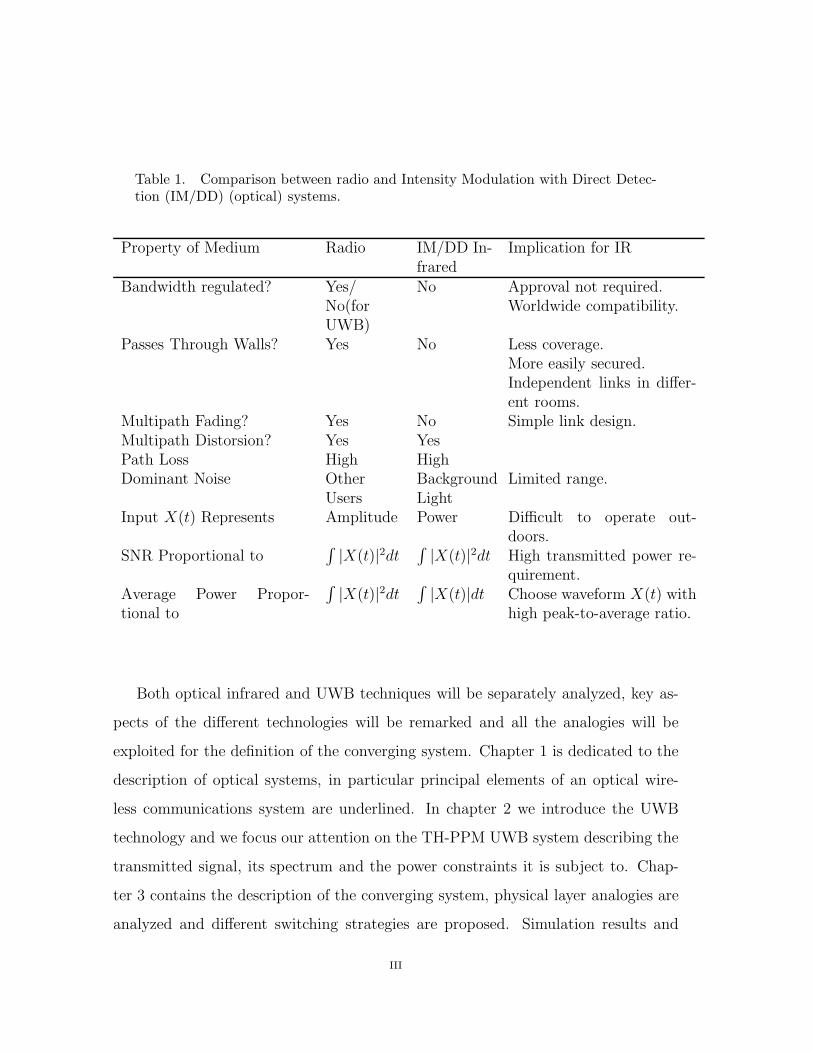
Table 1. Comparison between radio and Intensity Modulation with Direct Detec-tion (IM/DD) (optical) systems.
Property of Medium Radio IM/DD In-frared
Implication for IR
Bandwidth regulated? Yes/ No Approval not required.No(forUWB)
Worldwide compatibility.
Passes Through Walls? Yes No Less coverage.More easily secured.Independent links in di!er-ent rooms.
Multipath Fading? Yes No Simple link design.Multipath Distorsion? Yes YesPath Loss High HighDominant Noise Other
UsersBackgroundLight
Limited range.
Input X(t) Represents Amplitude Power Di"cult to operate out-doors.
SNR Proportional to!|X(t)|2dt
!|X(t)|2dt High transmitted power re-
quirement.Average Power Propor-tional to
!|X(t)|2dt
!|X(t)|dt Choose waveform X(t) with
high peak-to-average ratio.
Both optical infrared and UWB techniques will be separately analyzed, key as-
pects of the di!erent technologies will be remarked and all the analogies will be
exploited for the definition of the converging system. Chapter 1 is dedicated to the
description of optical systems, in particular principal elements of an optical wire-
less communications system are underlined. In chapter 2 we introduce the UWB
technology and we focus our attention on the TH-PPM UWB system describing the
transmitted signal, its spectrum and the power constraints it is subject to. Chap-
ter 3 contains the description of the converging system, physical layer analogies are
analyzed and di!erent switching strategies are proposed. Simulation results and
III

conclusions represent the content of chapter 4.
IV

Acknowledgements
Desidero ringraziare i miei genitori Luciano e Valeria e dedicare a loro questo mio
lavoro. Con il loro costante aiuto, fatto di telefonate comprensive e di qualche visita
fugace hanno saputo rendere decisamente meno duro questo mio percorso caratte-
rizzato, come mia abitudine, dal voler fare contemporaneamente molte piu cose di
quelle che dovrei complicandomi non poco la vita. Un ringraziamento speciale va a
Sabina, una splendida realta, che mi ha supportato nei momenti di"cili sapendomi
dare la sicurezza necessaria per poter continuare al meglio, che oramai dopo tanti
anni sa esattamente cosa dirimi al momento giusto e con la quale ho condiviso dei
momenti indimenticabili. Grazie. Non posso di certo non ringraziare i miei fratelli,
Alberto, Viola e Filippo che non sono mai mancati quando avevo un problema e
che mi hanno sempre incoraggiato. Ringrazio i miei amici, Paolo, Paola, Federica e
tutti gli altri con i quali ho condiviso questi bellissimi anni di universita fatti di bei
momenti di divertimento ma anche di tremende nottate passate a studiare insieme
a casa di qualcuno di noi. Grazie al mio Relatore, la Prof. Di Benedetto che ha cre-
duto in me e che mi ha dato la possibilita di realizzare questo lavoro. Grazie anche
al mio Correlatore, il Dr. De Nardis che nonostante la mia invadente ed insistente
richiesta di spiegazioni mi ha sempre puntualmente risposto.
V
Contents
Summary I
Acknowledgements V
1 Optical Communications 1
1.1 Historical Overview & State of the Art . . . . . . . . . . . . . . . . . 1
1.1.1 Basic Concepts in Optics . . . . . . . . . . . . . . . . . . . . . 11
1.1.2 Properties of the Light . . . . . . . . . . . . . . . . . . . . . . 13
1.1.3 Magnitudes and Units . . . . . . . . . . . . . . . . . . . . . . 15
1.2 Concepts of optical communications . . . . . . . . . . . . . . . . . . . 21
1.2.1 Optical Emitters . . . . . . . . . . . . . . . . . . . . . . . . . 30
1.2.2 The real optical channel . . . . . . . . . . . . . . . . . . . . . 35
1.2.3 Optical Receivers . . . . . . . . . . . . . . . . . . . . . . . . . 46
1.3 AIr MAC Protocol . . . . . . . . . . . . . . . . . . . . . . . . . . . . 51
2 Ultra-wide band communications 53
2.1 Historical Overview & State of the Art . . . . . . . . . . . . . . . . . 53
2.2 Principles of Impulse Radio in UWB communications . . . . . . . . . 56
2.2.1 Power Spectral Density of IR-TH-PPM UWB signal . . . . . . 59
2.2.2 Emission masks . . . . . . . . . . . . . . . . . . . . . . . . . . 62
2.3 UWB communications at low data rate . . . . . . . . . . . . . . . . . 66
VI

2.3.1 Multi User Interference (MUI) . . . . . . . . . . . . . . . . . . 67
2.4 Narrowband interference (NBI) onto UWB systems . . . . . . . . . . 76
2.5 MAC Protocols for Low Data Rate UWB . . . . . . . . . . . . . . . . 81
3 convergence IR-UWB 89
3.1 convergence IR-UWB . . . . . . . . . . . . . . . . . . . . . . . . . . . 89
3.2 Switching physical layer . . . . . . . . . . . . . . . . . . . . . . . . . 90
3.2.1 Energy consumption for UWB systems . . . . . . . . . . . . . 92
3.2.2 Optical Quantum Limit . . . . . . . . . . . . . . . . . . . . . 93
3.2.3 Modified-Quantum Limit . . . . . . . . . . . . . . . . . . . . . 95
3.2.4 Di!use wireless optical channel performance using OOC . . . 97
3.3 MAC for Low Data Rate Impulsive systems . . . . . . . . . . . . . . 98
4 Simulation results and Conclusions 101
4.1 The pulse collision model validation . . . . . . . . . . . . . . . . . . . 101
4.2 Potential Scenarios . . . . . . . . . . . . . . . . . . . . . . . . . . . . 104
4.3 Simulated scenario . . . . . . . . . . . . . . . . . . . . . . . . . . . . 105
4.4 Simulation results . . . . . . . . . . . . . . . . . . . . . . . . . . . . . 106
4.4.1 UWB system . . . . . . . . . . . . . . . . . . . . . . . . . . . 107
4.4.2 DWO system . . . . . . . . . . . . . . . . . . . . . . . . . . . 108
4.4.3 CIRCUS system . . . . . . . . . . . . . . . . . . . . . . . . . . 109
4.5 Conclusions . . . . . . . . . . . . . . . . . . . . . . . . . . . . . . . . 110
Bibliography 113
VII
List of Tables
1 Comparison between radio and Intensity Modulation with Direct De-
tection (IM/DD) (optical) systems. . . . . . . . . . . . . . . . . . . . III
1.1 Main Properties of the basic optical wireless links. . . . . . . . . . . . 9
1.2 Comparison between LEDs and LDs. . . . . . . . . . . . . . . . . . . 32
2.1 Average Power Limits set by FCC in the U.S. for Indoor UWB Devices. 65
2.2 Average Power Limits set by FCC in the U.S. for Outdoor UWB
Devices. . . . . . . . . . . . . . . . . . . . . . . . . . . . . . . . . . . 65
2.3 Maximum e.i.r.p. densities in the absence of appropriate mitigation
techniques, document released by the EC in 2007. . . . . . . . . . . . 66
VIII
List of Figures
1.1 Optical telegraph station at Metz, France (about 1830). . . . . . . . . 2
1.2 The Tyndall experiment. . . . . . . . . . . . . . . . . . . . . . . . . . 3
1.3 The Maiman Laser. . . . . . . . . . . . . . . . . . . . . . . . . . . . . 4
1.4 Donald Keck, Robert Maurer, and Peter Schultz from Corning Glass
Works, creators of the first practical optical fiber. (Photo from Corn-
ing Glass Inc.) . . . . . . . . . . . . . . . . . . . . . . . . . . . . . . . 6
1.5 Example of a FSO system interconnecting di!erent buildings to the
fiber backbone. . . . . . . . . . . . . . . . . . . . . . . . . . . . . . . 8
1.6 The electromagnetic spectrum. . . . . . . . . . . . . . . . . . . . . . . 11
1.7 Image formation by simple lens. . . . . . . . . . . . . . . . . . . . . . 18
1.8 Types of simple spherical lenses. . . . . . . . . . . . . . . . . . . . . . 19
1.9 Parallel rays of light brought to a focus by a positive thin lens. . . . . 20
1.10 Incident rays on a negative thin lens (diverge as if coming from a
point F on the left). . . . . . . . . . . . . . . . . . . . . . . . . . . . . 20
1.11 General scheme of an optical communication system. . . . . . . . . . 22
1.12 Common binary modulation schemes. . . . . . . . . . . . . . . . . . . 23
1.13 PSD of common binary modulation schemes. . . . . . . . . . . . . . . 23
1.14 (a) and (b) two di!erent OOC codewords belonging to the (32,4,1,1)
family, (c) auto-correlation, (d) cross-correlation. . . . . . . . . . . . . 28
1.15 Section diagram of an optical fiber (left) and a bunch of fibers (right). 36
IX

1.16 FSO system bandwidth demand vs covered distances. . . . . . . . . . 38
1.17 Example of di!use optical system. . . . . . . . . . . . . . . . . . . . . 41
1.18 Path Loss of an indoor optical system for both LOS and NLOS cases. 42
1.19 Optical spectra of common ambient infrared sources scaled to have
the same maximum value. . . . . . . . . . . . . . . . . . . . . . . . . 44
1.20 Example of two di!erent non-imaging hemispherical optical concen-
trators: a) with a planar filter and b) with and hemispherical filter. . 50
1.21 a) Low Impedance Amplifier , b) High Impedance Amplifier and c)
Trans-Impedance Amplifier. . . . . . . . . . . . . . . . . . . . . . . . 52
2.1 Transmission scheme for a PPM-TH-UWB. . . . . . . . . . . . . . . . 58
2.2 Example of UWB TH-PPM transmitted signal with Ns=5, average
transmitted power=-30dB, Ts=3ns, Tc=1ns, Nh=3, Np=5, Tm=0.5ns,
!=0.25ns and "=0.5ns. . . . . . . . . . . . . . . . . . . . . . . . . . . 60
2.3 PSD of an IR-TH-PPM UWB signal. . . . . . . . . . . . . . . . . . . 61
2.4 FCC indoor emission mask for UWB devices (FCC,2002). . . . . . . . 62
2.5 FCC outdoor emission mask for UWB devices (FCC,2002). . . . . . . 63
2.6 Linear model for the conditional probability of error Prob(Zmui <
!y|y,Nc, given y and Nc according to the Pulse Collision Model. . . . 74
2.7 Spectrum overlapping of the narrowband interferers in UWB systems. 77
2.8 An example of Superframe structure for 802.15.4 MAC. . . . . . . . . 83
2.9 UWB2 MAC protocol packet structures, a) Link Establish (LE) packet,
b) Data packet and, c) Link Confirm (LC) packet. . . . . . . . . . . . 87
3.1 BER variation due to a di!erent time duration of the transmitted
optical pulse with the same average transmitted power of 1mW and
10 nodes randomly positioned within a square room of 12mx12m. . . 96
4.1 BER vs. Ns for di!erent populated networks, according to the pulse
collision model increasing Ns does not improve the performance. . . . 102
X
4.2 Average number of interfering packets Ni as a function of the number
of pulses per bit Ns. Maintaining fixed Ts while increasing Ns cause
more collisions. . . . . . . . . . . . . . . . . . . . . . . . . . . . . . . 103
4.3 Average number of interfering packets Ni as a function of the number
of pulses per bit Ns; in this case Ts is reduced with increasing Ns,
thus the bitrate Rb remains approximately of 1Mbps. . . . . . . . . . 103
4.4 Throughput in the case of UWB physical layer with Ns = 3 and Ns =
5 for a network of 10 nodes with NLOSprobability=0.3 as a function of
the power spectral density of a narrow band interferer NNBI . . . . . . 107
4.5 Energy consumption for each node of the UWB network as a function
of the NBI PSD. . . . . . . . . . . . . . . . . . . . . . . . . . . . . . 108
4.6 Throughput in the case of two di!erently populated networks with
NLOSprobability set to 0.3 as a function of the transmitted optical
power of the LED. . . . . . . . . . . . . . . . . . . . . . . . . . . . . 109
4.7 An approximation that shows the dual system theoretical behaviour
if a narrow band interference would a!ect the UWB physical part. . . 110
XI

Chapter 1
Optical Communications
1.1 Historical Overview & State of the Art
Since ancient times light has been used to convey information from source to desti-
nation. Fires, torches, and the reflection of sunlight over a mirror, have been used,
for example, to transmit alerts of approaching dangers such as enemy armies. A
human observer acted as the receiver by visually perceiving optical signals. In more
complex systems, the transmission process included information coding, as in navy
flags for example, where a person waves arms or flags in di!erent patterns to rep-
resent letters and numbers. The introduction of mechanical tools allowed shapes
and patterns to grow larger and, therefore, be identified by an observer at larger
distances than with human transmitters. The first significant example adopting this
strategy was invented in the 1790’s by French engineer C. Chappe and was named
optical telegraph (see Figure 1.1). The system, consisting in a series of semaphores
mounted on towers where human operators relayed messages from one tower to the
next, was much faster than hand-carried messages, but was replaced by mid-19th
century by the electric telegraph, leaving a scattering of “Telegraph Hills” as its
most visible legacy.
1

1 – Optical Communications
After the electrical telegraph was established, J. Leseurre introduced in 1855 the
Figure 1.1. Optical telegraph station at Metz, France (about 1830).
mirror heliograph that is a system capable of transmitting light beams after multiple
reflections of sunlight over a set of mirrors in the direction of an intended recipient.
The beam was keyed “on” and “o!” by means of a shutter or tilting mirror, and
allowed thus the transmission of Morse coded messages. The system was operated
at a speed of 5 to 12 words per minute, depending on Morse skills of the operator.
During late 1800’s, heliographs were used in several countries, typically for military
applications.
Another breakpoint in the history of optical communications was the discovery
of the phenomenon known as total internal reflection that is the confinement of light
in a material surrounded by a medium with lower refractive index, such as glass in
air. In the 1840’s, D. Colladon and J. Babinet showed that light could be guided
along jets of water for fountain displays. J. Tyndall popularized light guiding in an
experiment that he first demonstrated in 1854, in which light was guided in a jet of
water flowing from a tank (see Figure 1.2).
As regards the use of light for data transmission, it is as back as in 1880 that
2

1.1 – Historical Overview & State of the Art
Figure 1.2. The Tyndall experiment.
A. G. Bell patented an optical wireless telephone system called the Photophone.
Bell dreamed of sending signals through the air, but experienced that the atmo-
sphere did not transmit light as reliably as wires carried electricity. In the following
decades, light was used for very limited and specific applications, as for example sig-
nalling between ships, and optical communication systems, such as the experimental
Photophone donated by Bell to the Smithsonian Institution, languished on the shelf.
The next important milestone was reached in 1958, about 80 years after the
Photophone, when L. Schawlow and C. H. Townes published their theoretical re-
sults on the possibility of amplifying light by stimulated emission of radiation. In
their study, Schawlow and Townes were actually considering microwave frequencies,
but their results opened the way to investigations in the infrared and visible spec-
trum. This concept later formed the basis for the development of laser devices. As
a natural consequence, research and development intensified for creating practical
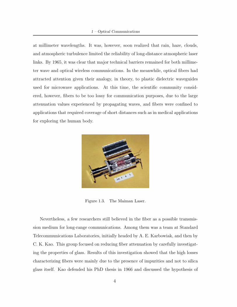
devices, and it was in 1960 that T. Maiman invented the first ruby-based practical
laser (see Figure 1.3). The device was identified as a possible emitter in wireless
optical communication systems, since air is far more transparent at optical than
3
1 – Optical Communications
at millimeter wavelengths. It was, however, soon realized that rain, haze, clouds,
and atmospheric turbulence limited the reliability of long-distance atmospheric laser
links. By 1965, it was clear that major technical barriers remained for both millime-
ter wave and optical wireless communications. In the meanwhile, optical fibers had
attracted attention given their analogy, in theory, to plastic dielectric waveguides
used for microwave applications. At this time, the scientific community consid-
ered, however, fibers to be too lossy for communication purposes, due to the large
attenuation values experienced by propagating waves, and fibers were confined to
applications that required coverage of short distances such as in medical applications
for exploring the human body.
Figure 1.3. The Maiman Laser.
Nevertheless, a few researchers still believed in the fiber as a possible transmis-
sion medium for long-range communications. Among them was a team at Standard
Telecommunications Laboratories, initially headed by A. E. Karbowiak, and then by
C. K. Kao. This group focused on reducing fiber attenuation by carefully investigat-
ing the properties of glass. Results of this investigation showed that the high losses
characterizing fibers were mainly due to the presence of impurities and not to silica
glass itself. Kao defended his PhD thesis in 1966 and discussed the hypothesis of
4

1.1 – Historical Overview & State of the Art
using, in theory, single-mode fibers with attenuation below 20 dB/km for long-range
communications. The first usable optical fiber was invented in 1970 by researchers
R. D. Maurer, D. B. Keck, P. Schultz, and F. Zimar working for American glass
maker Corning Glass Works (see Figure 1.4). They manufactured a fiber with an
attenuation of 17 dB/km, by doping silica glass with titanium. Based on this discov-
ery, the first experimental fiber optic communication system was installed in 1976.
Using a gallium-arsenide semiconductor laser, the AT&T US company installed an
experimental 2000-meter-long (1.25 miles) fiber optic cable under the streets of At-
lanta, Georgia. The technology evolved so fast that in 1980 with similar emitters the
degree of purity of the fiber allowed a 240 km coverage; if the sea was as transparent
as such a fiber, one would see the bottom of the Pacific ocean as clearly as in a pool,
even in the deepest abyssal zones. By mid-80’s, the fiber replaced wired-copper,
microwave and satellite links. The first transatlantic telephone cable using optical
fibers named TAT-8 was put in operation in 1988 by AT&T. It initially carried
40,000 telephone circuits (simultaneous calls) between the US and France, o!ering
a capacity of (2+1)x280 Mb/s, indicating that two fibre pairs with a capacity of 280
Mb/s each were available to provide normal service, while another fibre pair with
similar capacity was available for back-up purposes .
At this stage, amplification was electrical. Performance i.e. signal-to-noise, was
mainly limited by amplifiers rather than by lasers and fibers. The evolution towards
systems covering larger distances at higher transmission rates could be made possi-
ble by reaching pure optical amplification. In 1985, S. B. Poole, from Southampton
University, UK, discovered that it was possible to create a full-optical amplifier by
doping glass fibers with Erbium. Using this approach, D. Payne and P.J. Mears,
also from Southampton University, and E. Desurvire from the Bell Laboratories,
developed a full-optical fiber link.
5

1 – Optical Communications
Figure 1.4. Donald Keck, Robert Maurer, and Peter Schultz from Corning GlassWorks, creators of the first practical optical fiber. (Photo from Corning Glass Inc.)
In the 90’s, cable television adopted fiber optics to enhance network reliability.
Computers and Local Area Networks (LANs) started using fiber at about the same
period of time. Industrial links were among the first to be set, since features such
as noise immunity and low attenuation made it ideal for factories and storage net-
works. Several other applications developed fast: on-board aircraft and satellites
copper cable replacement thanks to the reduced weight, ships and automobile data
buses, surveillance systems for security, links for consumer digital stereo, etc.
Today’s fiber transmission standard rates could be reached thanks to the intro-
duction of multiplexing, and in particular Wavelength Division Multiplexing (WDM)
techniques. In a similar way of Frequency Division Multiplexing (FDM) for Radio
Frequencies (RF) channels, WDM allowed for the transmission of di!erent wave-
lengths of light simultaneously over a single fiber, maximizing thus the total band-
width per fiber. Systems such as TAT-14 entered the service by the end of 2000,
o!ering a capacity of (4+4)x160 Gb/s (over 1500 times more capacity than 12 years
earlier with TAT-8).
6

1.1 – Historical Overview & State of the Art
In the recent past, the possibility of using wireless optical transmissions, also
referred to as free-space optical communications (FSO), as an alternative (or a sup-
plement) to fiber optics connections came back to surface. The main reason for this
interest is the possibility to have a license-free high-speed link where cable transmis-
sions will be logistics di"culties for deploying the fiber. FSO and fiber transmissions
use similar light wavelengths, reach similar transmission bandwidths, and adopt sim-
ilar modulation techniques. Point-to-point broadband wireless optical connections
with transmission rates up to 1 Gb/s are nowadays practicable. A common scenario
of application for FSO consists in wideband connections between two points, for
example two buildings, where the installation of a wired connection would either
be impossible or too expensive, and where a microwave radio based system would
not o!er the necessary bandwidth (see Figure 1.5). Well-designed FSO systems are
typically characterized by outage probability of 10−3 at 500-2000 m ranges, and have
been installed in several cities all around the world for example in the surrounding
area of Milan, in Italy [3] . A feasible use of an FSO system is the installation of the
“last mile” link from the fiber backbone directly to the client or between di!erent
buildings [4]. FSO system performance is primarily dependent upon the climatology
and physical characteristics of the installation location. Even if modern systems can
work with every kind of climate [5], atmospheric attenuation typically dominated by
fog, low clouds, rain, snow and dust is the major weakness of this systems. Turbu-
lences can also cause atmospheric scintillation, which introduces fluctuations in the
received light intensity. Alignment between transmitter and receiver is another key
factor; FSO emitters transmit in fact highly directional and narrow light beams that
must impinge upon the aperture of the receiver. A typical FSO emitter transmits
one or more light beams; each of these is about 5-8 cm in diameter at the trans-
mitter and typically spreads to roughly 1-5 m in diameter at a range of 1 km. This
e!ect might prove to be disastrous when, for instance, either the transmitter or the
7

1 – Optical Communications
receiver moves unexpectedly, even by a slight amount. Buildings, for example, are
constantly in motion due to a variety of factors, including thermal expansion, wind
sway, and vibration. Because of the narrowness of the transmitted beam and the
restricted receiver Field Of View (FOV), building sway can a!ect link alignment
and interrupt communication. Since FSO systems can be easy installed they can
be used in mobile/nomadic situations (e.g seminars, meetings or events) but also
the creation optical bridges between di!erent locations for disaster management is
a possibility.
Figure 1.5. Example of a FSO system interconnecting di!erent buildingsto the fiber backbone.
A di!erent scenario of application for wireless optical transmissions consists in
communications based on light di!usion. These systems are suitable for low/medium
baud-rates links for cable replacement, with a small degree of mobility. Optical
wireless links between portable devices, as well as for in-house applications, have
been a hot research topic [6],[7],[1],[8],[9],[10], in parallel with the development of RF
solutions in the same framework. In di!use systems, the link is always maintained
between any transmitter and any receiver in the same vicinity by reflecting the
transmitted information-bearing light o! reflecting surfaces such as ceilings, walls
and furniture. The transmitter and the receiver are not necessarily in visibility, thus
8

1.1 – Historical Overview & State of the Art
Non Line-of-Sight (NLOS) links are fully exploited. Table 1.1 summarizes the main
properties of directed and di!use links.
Table 1.1. Main Properties of the basic optical wireless links.
Type of link Tx FOV Rx FOV ConnectionAdvantage Disadvantage Implementation
Directed Narrow Narrow LOS High speed Shadowing ComplexDi!use Wide Wide Reflections High Cov-
erageLow speed Simple
Di!use systems are mainly used for indoor transmissions and the di!use opti-
cal channel is exposed to ambient light sources like daylight, tungsten light and
fluorescent lamps. In general, there is an high level of stationary or slowly fluctu-
ating ambient light generating shot noise in the receiving photodiode. In addition,
artificial-light sources also emit rapid fluctuating components associated with higher
harmonics of the mains frequency; this have to be eliminated by electrical filtering.
Part of the incidental ambient light can be mitigated by optical filtering.
Nowadays, there is no real competition between wireless RF and wireless opti-
cal systems. RF systems are well established, cheap and robust, but there are some
specific scenarios in which wireless optical systems may be competitive. F.R. Gfeller
[6] proposed for example using infrared systems as an alternative to RF for portable
terminals in indoor applications. An interesting use of optical di!use systems that
is becoming popular is Visible Light Communication (VLC) that is communicating
via 380-700 nm LEDs, due to the inherently di!use optical source, the safety issue
is minimized. Furthermore provided that the emitted light is visible those systems
could be used simultaneously lighting and communication. The idea of bringing
these two worlds together was recently re-invigorated through the emergence of
white-light LEDs, which o!er a considerable modulation bandwidth of about 20
9
1 – Optical Communications
MHz [8] and are low cost elements [11]. As a matter of fact, several manufacturers
and research groups produce nowadays wireless optical products for a wide range
of applications. Nowadays optical communications are integrated into the commu-
nication world thanks to the definition of standards classified in correspondence to
channel types that is fiber, FSO, and di!use optical wireless.
Communication networks that use the fiber as the transmission medium.
There are several standards developed by international organizations for di!erent
application scenarios. The North American Telecommunications Industry Associ-
ation (TIA) has promoted the FO-4 Engineering Committee on Fiber Optics as a
responsible for the development and maintenance of fiber optic components, sub-
systems, systems, and network technology standards. For example a sub-committee
of FO-4 established that the recent TAT-14 submarine transatlantic cable system
should use WDM with 16 wavelengths per fiber pair, giving an aggregate capacity
of about 9,700,000 circuits per fiber. Other standards are promoted by the IEEE
and OSA (Optical Society of America): these were adopted for several applications
such as cable TV and hybrid networks, LAN, Metropolitan Area Network (MAN),
and Wide Area Network (WAN), Synchronous Digital Hierarchy (SDH) networks,
submarine links.
FSO Free space optical systems are not intended to be standardized.
Di!use Wireless Optical (DWO) For Di!use Wireless optical systems two
main commercial standards are available: the IrDA standard for computer and pe-
ripherals interconnection (also used for connections between cellular phones or palm
computers) and the IEEE 1073 standard for medical instrumentation interconnec-
tion.
10

1.1 – Historical Overview & State of the Art
1.1.1 Basic Concepts in Optics
Light is an electromagnetic radiation characterized by periodically varying electric
and magnetic fields that are mutually orthogonal and move at the speed of light.
When travelling through space or being reflected, light behaves like a wave. When
emitted from, or absorbed by, materials, it behaves like a particle. As a general
concept, an electromagnetic radiation is characterized by three parameters (ampli-
tude, wavelength or frequency, and phase). Wavelength is defined as “the distance
over which the wave repeats itself” and is represented by #. The time required to
complete one cycle of the wave, is called period of the wave. The frequency of the
wave is the number of cycles of the wave contained in one second and is represented
by $. Electromagnetic radiations are classified as a function of their wavelength; the
infinite possible values of wavelengths, and corresponding radiations, are commonly
referred to as the electromagnetic spectrum (see Figure 1.6) .
Figure 1.6. The electromagnetic spectrum.
As it is shown in the Figure we can classify radiations with respect to the in-
creasing frequencies (reducing wavelengths):
11

1 – Optical Communications
• radio waves in the region of wavelengths between 300’000 and 0.3 meters,
corresponding to frequencies between 1 kHz and 1 GHz)
• microwaves, wavelengths from about 0.3 meters to about 0.0003 meters
• infrared from about 300 to 0.7 µm
• visible light, from 0.4 to 0.7 µm
• ultraviolet from about 0.4 to 0.01µm
• x-rays from about 0.01µm to about 10E-4µm
• gamma rays, wavelengths shorter than about 10E-4µm
These last very short-wavelength, high-energy radiations show interactions with
the matter that are more particle-like than wave-like. Indeed, gamma rays are
usually characterized in terms of their photon energy, above 103 keV (Gamma rays
are the most energetic form of electromagnetic radiation). In the following, we will
focus on the so-called optical spectrum including infrared, visible and ultraviolet:
• Infrared (IR) is the portion of the electromagnetic spectrum with wavelengths
from about 300 to 0.7 µm (over the red part of the visible light). It can be
further subdivided into far, intermediate and near infrared. Far and interme-
diate infrared, corresponding to the longer wavelengths, are used for thermal
imaging, while the near infrared region is useful not only for optical commu-
nications but for detection and identification of superficial materials.
• Visible light (VIS) is the rather narrow but important region of the electro-
magnetic spectrum to which the typical human eye is sensitive. It goes from
the red (near to infrared) to the blue (near to ultraviolet).
12
1.1 – Historical Overview & State of the Art
• Ultraviolet (UV) is a more energetic electromagnetic radiation that covers the
region from about 0.4 to 0.01 micrometers. It is capable of inducing photo-
chemical reactions and is generally detrimental to organic materials. Far UV
is strongly absorbed by ozone, (also by oxygen) and is also strongly attenuated
by normal glass lenses.
The transmission characteristics of several materials as well as the absorption for
di!erent atmospherical components in the near infrared region have been extensively
analyzed. As a result of this analysis, three wavelength regions have been identified,
that are characterized by a low attenuation. These regions are called transmission
windows. The first window has wavelengths between 700 and 900 nm; the second
includes wavelengths from 1200 to 1300 nm, while the third one is centered around
1550 nm. The existence of such transmission windows has driven the design of
emitters and receivers, that typically operate in one of the windows.
1.1.2 Properties of the Light
Polarization As mentioned above, light consists in wave variations of mutually
orthogonal electric and magnetic fields. As a consequence, if the direction of one of
these fields is known, the direction of the other is also known. The polarization of
light defines the orientation of the electric field in space. The following terms are
commonly employed in the description of polarized light:
• Unpolarized light has no specific orientation of electric field. The direction of
the electric field varies randomly at approximately the frequency of light.
• Plane-polarized light is characterized by an electric field that oscillates in one
plane only.
• In vertically-polarized light the plane of the electric field is vertical and moves
13

1 – Optical Communications
up and down in the plane. In horizontally-polarized light the plane that con-
tains the electric field is horizontal.
• In circularly-polarized light, the direction of the electric field is neither random
nor confined to a single plane. The direction of the electric field of circularly-
polarized light sweeps out a circle during each period of the wave.
Coherence Can be defined for light waves as the condition that exists when all
the light waves are in phase. The coherence can be defined as follows: if we consider
a set of light waves emitted at the same instant in the same point in space, these
light waves are temporally coherent if, given an observation point in space and an
observation instant in time, all the light waves show the same value of the electrical
field. In the case of a light source, there are two main causes of lack of coherence:
• Temporal The variation of the electrical field in a light wave depends on the
frequency (or, equivalently, wavelength) of the light wave. Since an optical
source emits several light waves at the same time, the more nearly the output
of the source approximates a single frequency (monochromaticity), the more
temporally coherent is the emitted light.
• Spatial A light source emits arrays of photons (each of them corresponding
to a light wave), that are supposed to depart at the same time by the entire
area of emission. In a light source characterized by a large active area of
emission, however, di!erent sections of the area of emission will emit photons
belonging to the same array in di!erent times, causing a lack of coherence. As
a consequence, the smaller is the extent of a light source, that is the more it
resembles a point source, the greater the coherence of the emitted light.
Interference It occurs when a coherent light beam is divided into two parts and
later recombined. If the two waves are combined at a point at which they are 180◦
14
1.1 – Historical Overview & State of the Art
out of phase, the two electric fields cancel through a process called destructive inter-
ference producing a dark area. If both waves arrive in phase we have a constructive
interference, and their electric fields add to produce an area that has an increased
irradiance. If the two waves are of equal amplitude, the irradiance at this point is
four times that produced by either of the beams alone.
1.1.3 Magnitudes and Units
In this section we shall briefly describe the units and magnitudes that are com-
monly used in optical communications. We will focus on the international system of
units (usually called the SI, using the first two initials of its French name Systeme
International d’Unites ) The SI is maintained by a small agency in Paris, the In-
ternational Bureau of Weights and Measures (BIPM, for Bureau International des
Poids et Mesures ).
Luminous intensity Also known as candlepower is the light density emitted
within a very small solid angle, in a specified direction. The unit of measure is
candela (cd). In modern standards, the candela is the basic of all measurements of
light and all other units are derived from it.
Formally the Candela is defined to be the luminous intensity of a light source pro-
ducing single-frequency light at a frequency of 540 THz with a power of ( 1683·W/steradian),
or 18.3988mW over a complete sphere centered at the light source (a steradian is
defined as the solid angle that, given a sphere of radium R, determines on the sur-
face of the sphere a circle of area R2). The frequency of 540 THz corresponds to a
wave length of approximately 555.17nm. In order to produce 1 candela of single-
frequency light of wavelength #, a lamp would have to radiate ( 1683·V (λ)·W/steradian) ,
where V(#) is the relative sensitivity of the eye at wavelength #. These values are
defined by the International Commission on Illumination (CIE).
15
1 – Optical Communications
Luminous flux It corresponds to the time rate of flow of light. The unit of
measure is the lumen (lm). One lumen may be defined as the light flux emitted in
one unit solid angle by a one-candela uniform-point source. The lumen di!ers from
the candela in that it is a measure of light flux irrespective of direction. In fact, one
lumen equals to the intensity in candelas multiplied by the solid angle in steradians
into which the light is emitted. Thus the total flux of a one-candela light, if the light
is emitted uniformly in all directions, is 4% lumens. Note that a lumen is a measure
of optical power, as Watt is. The di!erence between lumen and watts relies in the
fact that lumen definition takes into account the human eye sensitivity. Therefore,
lights with the same power in watts, but di!erent colours have di!erent luminous
fluxes, because the human eye has di!erent sensitivity at di!erent wavelengths. At
a wavelength of 555 nm (maximum eye sensitivity) 1 Watt equals 683 Lm.
Very powerful sources of infrared radiation produce no lumen output, because
the human eye can not see it. However, if you need to calculate total power absorbed
by a surface (to estimate temperature increase, for example), you have to transfer
lumen flux to watt. This can be done by using a spectral luminous e"ciency curve
(V(#)).
Illumination Illumination is defined as the density of luminous flux on a surface.
This parameter shows how “bright” the surface point appears to the human eye.
The SI unit to measure illumination is lux (lx) and is defined as an illumination of
1 lm/m2.
Luminance or Brightness It is defined as the luminous intensity on a surface in
a given direction per unit of projected area of the surface. Luminance is especially
important because our eye only sees brightness, not illumination. It is proportional
to the object’s illumination, so a well illuminated object seems brighter. Luminance
can be expressed in many ways: using SI units we can express it in candelas per
16

1.1 – Historical Overview & State of the Art
unit of area or in lumens per unit of solid angle per unit of area. In the CGS system
we find the lambert (La) that is defined as the luminance of a surface that emits or
reflects one lumen/cm2. As it is a large unit, practical measurements tend to be in
millilamberts (mLa). A surface area having an intensity of 1 cd/m2 emits a total
light flux of (% · lmsr/m2 ); as a result: 1 La=3183.099 cd/m2.
Lambertian Surfaces It is a di!use reflector ideal. It is a surface that adheres to
Lambert cosine law, that states that the reflected or transmitted luminous intensity
in any direction from an element of a perfectly di!using surface varies as the cosine
of the angle between that direction and the normal vector of the surface. As a
consequence, the luminance of that surface is the same regardless of the viewing
angle. A good example is a surface painted with a good “matte” or “flat” white
paint. If a Lambertian surface is uniformly illuminated, like from the sun, it appears
equally bright form whatever direction you view it.
Lenses and Collimators Lenses are used in optical communications to change
the direction of rays of light (see Figure 1.7). Lenses are used for example for sep-
arating di!erent spots of light in order to avoid interferences, or for concentrating
light on a point in order to increase the active area at the receiver without increasing
other related parameters (as the spurious capacitance that severely limits the band-
width at the receiver). They can be used also as filters for avoiding the incidence
of signals out of the desired scope of wavelength. The e!ect of a lens on light is
embodied in Snell’s law of refraction. This law states that, in passing from a rarer
medium into a denser one, light is refracted toward the normal. In passing from a
denser to a rarer medium, light is refracted away from the normal. The degree of
bending or refracting is in accordance with the following equation:
n1 · sin&1 = n2 · sin&2 (1.1)
17

1 – Optical Communications
Where n1 and n2 are the indices of the two media, and &1 and &2 are the angles
of incidence and refraction, respectively.
Figure 1.7. Image formation by simple lens.
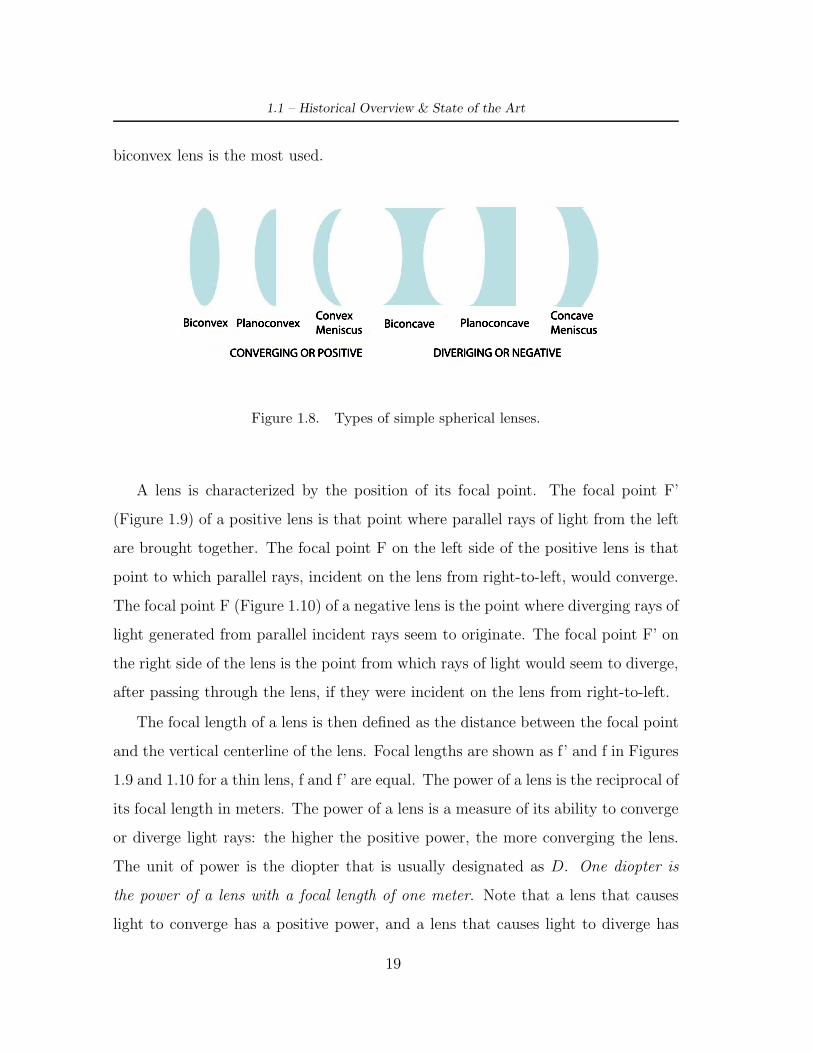
Lenses can be classified into two general types according to the e!ect they have
on a parallel beam of light. The two types are converging and diverging lenses.
Converging lenses Also are called “positive”, “plus”, or “convex” lenses. They
are thicker in the middle than at the edges. They cause both parallel rays of light
and diverging rays of light arriving at one side of the lens to converge on the opposite
side.
Diverging lenses Also known as “negative”, “minus”, or “concave” lenses and
are thinner in the middle than at the edges.
Diverging lens causes parallel rays of light to diverge or spread in opposite di-
rections on the other side of the lens. If rays initially are diverging toward such a
lens, they will be made to diverge even more strongly after they pass through the
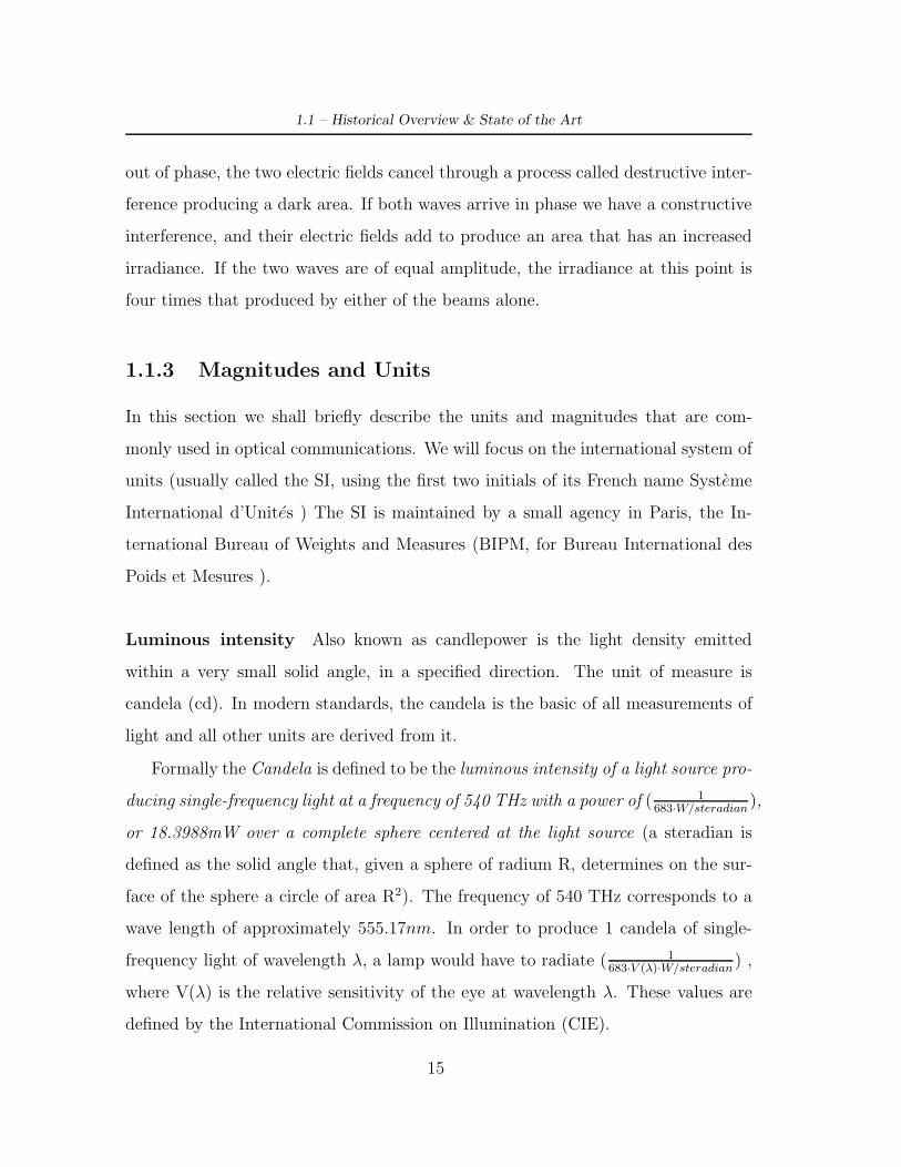
lens. Further subdivisions of these two basic types can be made according to the
curvature of the lens surfaces. Spherical lenses are lenses whose surfaces are spheri-
cal in shape. They can be classified into the six sub-types shown in Figure 1.8. The
18
1.1 – Historical Overview & State of the Art
biconvex lens is the most used.
Figure 1.8. Types of simple spherical lenses.
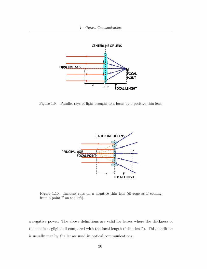
A lens is characterized by the position of its focal point. The focal point F’
(Figure 1.9) of a positive lens is that point where parallel rays of light from the left
are brought together. The focal point F on the left side of the positive lens is that
point to which parallel rays, incident on the lens from right-to-left, would converge.
The focal point F (Figure 1.10) of a negative lens is the point where diverging rays of
light generated from parallel incident rays seem to originate. The focal point F’ on
the right side of the lens is the point from which rays of light would seem to diverge,
after passing through the lens, if they were incident on the lens from right-to-left.
The focal length of a lens is then defined as the distance between the focal point
and the vertical centerline of the lens. Focal lengths are shown as f’ and f in Figures
1.9 and 1.10 for a thin lens, f and f’ are equal. The power of a lens is the reciprocal of
its focal length in meters. The power of a lens is a measure of its ability to converge
or diverge light rays: the higher the positive power, the more converging the lens.
The unit of power is the diopter that is usually designated as D. One diopter is
the power of a lens with a focal length of one meter. Note that a lens that causes
light to converge has a positive power, and a lens that causes light to diverge has
19
1 – Optical Communications
Figure 1.9. Parallel rays of light brought to a focus by a positive thin lens.
Figure 1.10. Incident rays on a negative thin lens (diverge as if comingfrom a point F on the left).
a negative power. The above definitions are valid for lenses where the thickness of
the lens is negligible if compared with the focal length (“thin lens”). This condition
is usually met by the lenses used in optical communications.
20

1.2 – Concepts of optical communications
1.2 Concepts of optical communications
The general scheme of an optical communication system can be depicted as in Figure
1.11. The input to the system is a digital, base-band data signal. The data input is
first processed in an electrical form at the transmitter by the transmitter electrical
processor, secondly transduced into an optical signal by the optical emitter, and
finally filtered and amplified by optical lenses. The output of the transmitter forms
the input to the optical channel. At the output of the channel the optical signal
that enters the receiver is corrupted by noise and interference. The receiver is
formed by a front-end optical filter and amplifier, followed by a receiver transducer
(the photodiode) that produces an electrical current that is processed by the final-
stage amplifier and treated as any electrical signal would be. In this section we
briefly analyze basic concepts related to the main blocks of Figure 1.11 and in
particular: modulation and coding carried out by the transmitter electrical processor
(section 1.2), transduction by the optical emitter (section 1.2.1), transmission over
a real optical channel a!ected by noise and interference (section 1.2.2), transduction
by the optical receiver (section 1.2.3), and amplification in the receiver electrical
processor (section 1.2.3). Optical filtering and amplification by lenses have already
been analyzed in the previous section.
Modulation and Coding
Modulation and coding schemes best suited for optical transmissions are commonly
based on intensity modulation/direct detection (IM/DD) schemes operating either in
the baseband or in shifted bands using electrical subcarriers. The information is then
conveyed by the instantaneous optical power at the output of the optical emitter.
At the receiver, a photodetector produces a current proportional to the received
instantaneous optical power. This optical power is proportional to the square of
the received electric field and is the integral over the photodetector surface of the
21

1 – Optical Communications
!"!#T%I#A"(%)#!**)%
)(TI#A" !,ITT!% "!-*!*
"!-*!*I-T!%.!%!-#!
)(TI#A".I"T!%*
!"!#T%I#A"(%)#!**I-/
)(TI#A" #0A--!"
-)I*!
I-T!%.!%!-#!
1ATA
1ATA
%!#!I2!%
T%A-*,ITT!%
(0)T)1I)1!
Figure 1.11. General scheme of an optical communication system.
received scattered optical power, similarly to what happens in a receiving antenna.
Popular baseband modulation schemes are On-O! Keying (OOK) with Non Return
to Zero (NRZ) and Return to Zero (RZ), Pulse Position Modulation (PPM). In
Figure 1.12 these di!erent binary modulation schemes are depicted: (a) in OOK
with NRZ, (b) OOK with RZ with a duty cycle of '=0.5, (c) 2-PPM, and (d) BPSK
subcarrier at a frequency equal to the reciprocal of the symbol duration.
For all baseband and single-carrier modulation schemes, we define B the first null
bandwidth of the Power Spectral Density (PSD) of the transmitted waveform X(t).
For multiple-subcarrier schemes, the bandwidth requirement B is the span from
dc to the first null in the highest-frequency subcarrier. We will present bandwidth
requirements B/Rb, i.e., normalized to the bit rate Rb. In Figure 1.13 the normalized
spectrum of the four di!erent binary schemes is provided. The power Pt is the
22
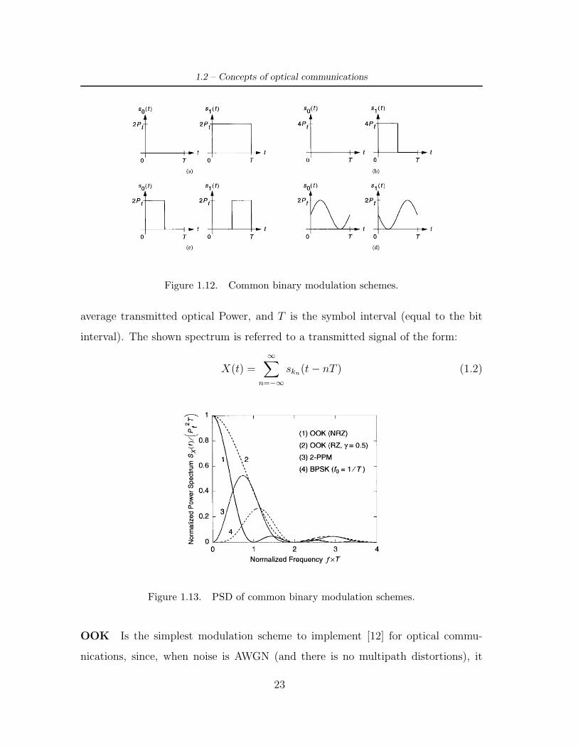
1.2 – Concepts of optical communications
Figure 1.12. Common binary modulation schemes.
average transmitted optical Power, and T is the symbol interval (equal to the bit
interval). The shown spectrum is referred to a transmitted signal of the form:
X(t) =∞"
n=−∞
skn(t ! nT ) (1.2)
Figure 1.13. PSD of common binary modulation schemes.
OOK Is the simplest modulation scheme to implement [12] for optical commu-
nications, since, when noise is AWGN (and there is no multipath distortions), it
23

1 – Optical Communications
only requires an ideal maximum-likelihood (ML) receiver. In this case the ML re-
ceiver consists in a continuous-time filter matched to the transmitted pulse shape,
followed by a sampler and a threshold detector. When using OOK with duty cycle
0 < ' < 1 the bandwidth requirement increments by a factor 1/', however this
increment provides a decrease of the average optical power necessary to meet the
BER target (usually 10−6 for di!use systems); the reason is that the increased noise
associated to this expanded bandwidth is outweighed by the 1/' increase in peak
optical power. Thus, OOK with RZ is usually preferred to NRZ in infrared systems.
PPM Pulse Position Modulation is an orthogonal modulation scheme that o!ers
a decrease in the average-power requirement compared to OOK, at the expense of
an increased bandwidth requirement. In particular L-PPM uses symbols consisting
of L time slots also referred to as chips. A constant power L · Pt is transmitted
within one chip while zero power is transmitted during the remaining L ! 1 chips,
thereby encoding log2 L bits. For a given bit rate, LPPM requires more bandwidth
than OOK by a factor Llog2 L , (e.g., 16PPM requires four times more bandwidth than
OOK), but PPM can achieve much greater immunity to neardc noise from fluores-
cent lamps than OOK. In the absence of multipath distortion, L-PPM yields an
average-power requirement that decreases steadily with increasing L; this average
power reduction makes PPM especially suitable for portable devices. On the other
hand, PPM presents two drawbacks: increased transmitter peakpower requirement,
and the need for both chip and symbol level synchronization. In the absence of
multipath distortion, an optimum ML receiver is a continuous-time matched filter
matched to one chip, whose output is sampled at chip rate. Each block of L samples
is passed to the decoder that can be an hard-decision or a soft-decision decoder
yielding log2 L information bits. The hard decision decoder is characterized by a
threshold detector that quantizes to “low” or “high” the samples and the decision
24

1.2 – Concepts of optical communications
is based on which sample is “high”. In the soft decision decoder the samples are
unquantized, and the block decoder chooses the largest of L samples.
Subcarrier Modulation In single-subcarrier modulation (SSM) a bitstream is
modulated onto a radio-frequency subcarrier, and this modulated subcarrier is mod-
ulated onto X(t), the instantaneous power of the infrared transmitter. Provided that
the optical signal must be non negative, a dc bias must be added if the subcarrier is
a sinusoid. The transmitted waveforms and PSD of a BPSK subcarrier are shown in
Figure 1.12(d) and 1.13, respectively, assuming a subcarrier frequency equal to the
bit rate. The required bandwidth of such a BPSK subcarrier is twice the bandwidth
of an OOK signal, while a QPSK subcarrier requires the same bandwidth as OOK.
After optical-to-electrical conversion at the receiver, the subcarrier can be demodu-
lated and detected using a standard BPSK or QPSK receiver.
Multiple access strategies and Optical Orthogonal Codes (OOC) In opti-
cal wireless communications MA schemes are mainly based on Time Division Mul-
tiple Access (TDMA) and Code Division Multiple Access (CDMA). In TDMA each
user is allowed to transmit only within a specified time interval (Time Slot). Di!er-
ent users transmit in di!erent Time Slots. With TDMA separation between users
is performed in the time domain, thus each transmitting user can use the whole
available frequency bandwidth. TDMA access technique can be use if the network
infrastructure is centralized with a coordinator node because it is necessary for the
coordinator to send to all nodes periodic reference burst aimed at defining the time
frames in which user can transmit. In real communications there are significant de-
lays between users, thus burst references are received with di!erent phases from this
reasoning guard times inside time slots are necessary. Moreover since each tra"c
25

1 – Optical Communications
burst is transmitted independently with an uncertain phase relative to the reference
burst, there is a need for a preamble at the beginning of each tra"c burst. This
preamble allows the receiver to estimate time and carrier phase. In CDMA tech-
niques each user has assigned a di!erent code (with uncorrelation properties) used
to encode data. Thus, di!erent user can transmit in the same time, exploiting the
whole available system bandwidth. Codes used in CDMA are called spreading codes
due to their particularity of spreading the bandwidth of the encoded signals, in fact
CDMA is based on spread-spectrum modulation. Tanks to the uncorrelation prop-
erty of the codes receiver can ideally perfectly recover the received signal knowing
the transmitter code. However transmissions of di!erent users of the networks are
not synchronized and this cause a partial loss of the uncorrelation of codes, that
become partially correlated. Partial correlation cannot be totally canceled but can
be mitigated by proper choice of the spreading codes. CDMA Channel capacity is
limited by the number if other users rather than by thermal noise. Furthermore,
in CDMA systems is necessary to perform a power control of the power level of
the transmitters, because a typical problem to deal with is near-far problem present
whenever all users transmit at the same power level (the received power is higher for
transmitters closer to the receiving antenna). An optical orthogonal code is a fam-
ily of (0,1) sequences with good auto- and cross-correlation properties [13],[14], [15],
[16]. OOC has thumbtack-shaped auto-correlation that enables the e!ective detec-
tion of the desired signal, and low-profiled cross-correlation make it easy to reduce
interference due to other users and channel noise. An OOC family is composed by
unipolar sequences suitable for OOK modulation. In general an (n,w,#a,#c) OOC is
a family of binary sequences of length n and weight w, with unipolar auto-correlation
and cross-correlation constraints #a and #c, respectively:
n−1"
t=0
xtxt+τ " #a (1.3)
26

1.2 – Concepts of optical communications
n−1"
t=0
ytxt+τ " #c (1.4)
for any x #= y $ C and any integer t. Aimed at reducing the correlation between
di!erent codes, the maximum cross correlation between any two di!erent code se-
quences should be zero. However, real binary (0,1) sequences, that is sequences for
truly positive systems, such as optical systems, can not achieve a cross-correlation
value 0, as the coincidences do not cancel out unlike in (+1,-1) sequences. Hence,
the minimum possible value of cross-correlation is 1. An (n,w,#a,#c) OOC C can be
alternatively considered as a family of w sets of integers modulo n in which each w
set corresponds to a codeword and the integers within each w set specify the nonzero
bits positions of the codeword. For instance, the simple OOC 1101000 is referred by
(7,3,1,1) but also {0,1,3}(mod 7). Then the auto-correlation and cross-correlation
properties can be reformulated, respectively as reported in [15]:
|(a + X) % (b + X)| " #a (1.5)
for X $ C and any a #= b mod(n), and
|(a + X) % (b + Y )| " #a (1.6)
for any X #= Y $ C and any a,b. Here a + X={a + x : x $ X} and all integers
under consideration are taken modulo n. In Figure 1.14 (a) and (b) two di!erent
codewords are shown. In (c) and (d) the auto-correlation and the cross-correlation
are, respectively depicted. The size of a code C that is |C|, denoted by M, is the
number of codewords in it. The cyclic shift of a codeword is not considered as
another codeword. Provided that is desirable to have OOC with the largest possible
number of codewords M, many studies in literature refers to upper and lower bounds
for OOC. The largest possible size of an (n,w,#a,#c) code is denoted by #(n,w,#a,#c).
A code that has maximum possible size M=#(n,w,#a,#c) is said to be an optimal
27

1 – Optical Communications
Figure 1.14. (a) and (b) two di!erent OOC codewords belonging to the (32,4,1,1)family, (c) auto-correlation, (d) cross-correlation.
code. There exists many di!erent methods to construct Optical Orthogonal Codes
like using Iterative Construction, Projective Geometry [15], but also using Error
Correcting Codes [16]. The use of OOC allow optical systems to increment the
system capacity in terms of the number of users that are transmitting at the same
time. Every information bit is encoded with the OOC and et receiver side correlator-
type decoders are used to neglect interfering signals. When the total number of users
goes up, the cross-correlation due to interfering users adds up to quickly to severely
degrade the system performance. To avoid this phenomenon, both w and n should
be increased simultaneously. If we increase only w fixing n, cross-correlation value
due to the interference can be lowered because. However, OOC has a very sparse
marks to keep the cross-correlations low, i.e. a number of zeros is much higher than
that of ones in the sequence. It means that the cross-correlation increases itself by
increasing only w. Anyway even increasing both w and n has a drawback, that is
a long signal processing time due to long n. After the correlator matched to the
single user signal, the receiver has threshold that is used to take decisions on the
28

1.2 – Concepts of optical communications
correlator output. The threshold $ value can be chosen under the condition:
0 " $ " w (1.7)
Two di!erent types of detector can be considered, soft-limiting and hard limiting.
The main di!erence is that in the soft-limiting detector, the contribution of a single
tap (the decoder is composed by tapped-delay lines) equals the number of pulses it
senses. If there are $ or more pulses, it outputs 1. In the hard limiting detector, the
contribution of a tap is one when it senses one or more pulses and zero otherwise.
The detector outputs a 1 when $ or more taps contribute 0 otherwise. The di!erence
between the two types of detectors is best illustrated when a small number of taps
on a single delay line are sensing a number of pulses. The soft-limiting detector
will produce a 1, while the hard-limiting type will not. Error probabilities for both
di!erent correlator can be found in [15] and [14].
Optical Orthogonal Codes will be used in in this work for system simulation
aimed at achieving a performance improvement as it will described in 3.2 and sub-
sequently shown by simulation results. As regards resource management and con-
trol (Medium Access Control (MAC)), Carrier-Sense Multiple Access by Collision
Avoidance (CSMA-CA) strategies are the most commonly adopted in commercial
systems. By these strategies, a transmitter senses the channel and avoids trans-
mitting when hearing the channel as busy. Other methods such as the well-known
Carrier-Sense Multiple Access by Collision Detection (CSMA-CD) are di"cult to
use in the optical context for similar problems to those experienced in RF wireless;
typically a transmitter that is actively transmitting is not able to detect another
transmission that is to detect a collision. The Advanced Infrared (AIr) Medium
Access protocol used by Irda will be further presented (1.3).
29
1 – Optical Communications
1.2.1 Optical Emitters
Two are the processes by which a source can emit light: spontaneous emission where
an electron makes a transition from a high energy state E2 to a lower energy state
E1 resulting in the emission of a photon, and stimulated emission where a photon,
with an energy equal to (E2!E1), interacts with an atom in the upper energy state,
causing it to return to the lower state and emit thus a second photon with same
phase, frequency, and polarization as the first. Semiconductor sources are based
on p-n junctions, and we will consider two di!erent light emitter types: the Light
Emitting Diode (LED) that produces scattered incoherent light and is electrically
simple to use and control, and the Light Amplification by Stimulated Emission of
Radiation (LASER) diode that produces a narrow beam of coherent light and re-
quires a more complex control than a LED.
Light Emitting Diodes (LEDs) produce light following the spontaneous emission
principle, while stimulated emission is the basic principle of operation of Light Am-
plification by Stimulated Emission of Radiation (LASER) based-devices that is laser
diodes. Basic properties of laser light are [17]:
• Monochromaticity This property is related to wavelength and thus colour.
A wavelength specifies the colour at which the laser lases. Ordinary coloured
light consists of a broad range of wavelengths covering a particular portion
of the visible-light spectrum. Laser beams consist of an extremely narrow
range of wavelengths, is thus common to refer to red, green, or blue lasers
(but not white laser). Laser beams are said to be nearly “monochromatic,”
or nearly “single-coloured.” Near-monochromaticity is a unique property of
laser light, meaning that it consists of light of almost a single wavelength.
Perfectly monochromatic light cannot be produced even by a laser, but laser
light is many times more monochromatic than the light from any other source.
30
1.2 – Concepts of optical communications
In some applications, special techniques are employed to further narrow the
range of wavelengths contained in the laser output and, thus, to increase the
monochromaticity.
• Intensity This property refers to the intensity of light. The energy emitted
by a laser in the narrow spectral region (colour) in which the laser lases, far
exceeds that of the sun or of any other known light source!
• Directionality and Coherence Common light sources, such as flashlights,
light bulbs, or the sun, emit energy in all directions. Devices such as auto-
mobile headlights and spotlights contain optical systems that collimate the
emitted light, such that it leaves the device in a directional beam; however,
the beam produced always diverges (spreads) more rapidly than the beam
generated by a laser. A laser, on the contrary, only emits light and only in a
very well defined direction. Moreover, common light sources emit light with a
random phase. In contrast, lasers emit light at only one phase, according to
the coherence property described in the previous section, that is all produced
photons are in phase (phase coherence), have the same wavelength (frequency
coherence or monochromaticity), and travel in the same direction (spatial co-
herence).
LEDs are inexpensive and can support input signals with bandwidths up to 100
MHz. Laser Diodes (LDs) produce a narrow beam of coherent light but they re-
quire more complex control and are more expensive than LEDs. A LD can support
input signals with bandwidths up to tens of GHz and can provide higher optical
power outputs than LEDs. Di!erent materials are used to manufacture lasers at
680, 800, 1300, and 1500 nm but the wavelength band between about 780 and 950
nm is presently the best choice for most applications of infrared wireless links, due
to the availability of low-cost LEDs and LDs, and because is coincides with the peak
31

1 – Optical Communications
responsivity of inexpensive, low-capacitance silicon photodiodes. The primary draw-
back of radiation in this band relates to eye safety: it can pass through the human
cornea and be focused by the lens onto the retina, where it can potentially induce
thermal damage, that is energy is absorbed by the tissue in the form of heat which
can cause localized, intense heating of sensitive tissues. The Human responsivity as
function of the wavelength is opaque beyond 1400 nm, unfortunately photodiodes
presents at this bands are much more expensive and has higher capacitance per unit
area than other more common LEDs.
Light emitted by a LEDs follows the spontaneous emission principle. LEDs are
simply biased p-n junctions crossed by a forward current. On the p side of the
junction empty electron states are occupied by injected electrons from the n side;
on the n side empty hole states are occupied by injected holes from the p side.
This increased concentration of minority carriers in the opposite type region leads
to recombination across the bandgap, releasing energy. This recombination can be
non-radiative (dissipated as heat) or radiative, resulting in a photon of energy Eg.
Generated photons are radiated in all directions with a wide wavelength range.
Table 1.2. Comparison between LEDs and LDs.
Characteristic LEDs LDs
Spectral width 25-100 nm < 10−5 to 5 nm(10-50 THz) (< 1MHz to 2 THz)
Modulation Bandwidth Tens of kHz to tens of MHz Tens of kHz to tens of GHzE/O Conversion e"ciency 10-20% 30-70%Eye Safety General considered eye-safe Must be rendered eye-safe,
especially for # < 1400 nmCost Low Moderate to high
32

1.2 – Concepts of optical communications
Di!erent colours LEDs are are available, there are white, blue, green, aqua, red,
orange, yellow, violet, ultra-violet, and infrared LEDs. Typical driving current is in
the order of mA and the luminous intensity of a LED is measured in Milli Candle
Power (mci); this intensity is measured in the most intense portion of the produced
beam. Use of LEDs is more common in wireless optical communication than in
fiber optics, because coupling su"cient power into a fiber is di"cult, thus regarding
the communication in fiber, LEDs are restricted to large core fibers. The most
common structure of LEDs is the so called Double Heterojunction (DH) or Double
Heterostructure. The Heterojunction is an interface between to semicondutcive
materials of di!erent bandgap energies (as opposed to a so called homojunction).
The p type layer of the p-n junction is a GaAs layer and the n type is a AlGaAs
Semiconductor lasers, most important for optical communications, are light emit-
ting diodes with a resonator cavity that is formed either on the surface of the diode
or externally. An electric current passing through the diode produces light emission
when electrons and holes recombine at the p-n junction in an area called active area.
The active area should be as small as possible in order to confine the laser output
and preserve coherence features. Dispersion in the laser output can be reduced by
means of special optical filters to produce a good beam shape. The original semicon-
ductor lasers were manufactured from crystals containing a junction between p- and
n-type gallium arsenide, but nowadays they use three or four elements from columns
III and V of the periodic table (the so-called III-V compounds). Examples of these
semiconductors are Al1-xGaxAs (aluminum gallium arsenide) or In1-xGaxAs1-yPy
(indium gallium arsenide phosphide). Lasers are used in several applications such
as optical-fiber communications, printers or CD players.
Given the quantum e"ciency of the diode (, that is the capability of the device in
emitting photons, the rate of emitted photons generated by radiative recombination
33

1 – Optical Communications
is:
Rp = (i
q(1.8)
where i is the forward bias current in Amperes and q is the charge on an electron in
Coulombs. Each photon has an energy of h$ Joules, so the optical power P measured
in Watts emitted by a LED is given by the product of Rp and h$:
P = Rp · h$ = (i
q· hc
#(1.9)
where c is speed of light and # is the wavelength characterizing the diode. Optical
power produced by a LED is thus intrinsically linear with input current and for
a given current, output optical power decreases when temperature increases. In
Table (1.2) presents a comparison between LEDs and LDs . Typical LEDs emit
light into semiangles (at half power) of 10◦-30◦, thus they are suitable for directed
transmission, in non directed systems like Di!use Wireless Optical systems, multiple
LEDs oriented in di!erent directions are employed. In general LEDs cost less and are
more safe than LD but they have several drawbacks like typically poor electro-optic
power conversion e"ciencies of 10-20% (against 30-70% of LDs) and broader spectral
widths, which require the use of a wide receiver optical passband, leading to poor
rejection of ambient light. The eye safety of infrared transmitters is governed by
International Electrotechnical Commission (IEC) standards [49]. It is desirable for
infrared transmitters to conform to the IEC Class 1 allowable exposure limit (AEL),
implying that they are safe under all foreseen circumstances of use, and require no
warning labels. At pulse repetition rates higher than about 24 kHz, compliance with
this AEL can be calculated on the basis of average emitted optical power alone. The
AEL depends on the wavelength, diameter, and emission semiangle of the source.
At present, the IEC is in the midst of revising the standards applying to infrared
transmitters. Based on proposed revisions, at 875 nm, an IrDA-compliant source
having an emission semiangle of 15◦ and diameter of 1 mm can emit an average
34

1.2 – Concepts of optical communications
power up to 28 mW. At the same wavelength, a Lambertian source (60◦ semiangle)
having a diameter of 1 mm can emit up to 280 mW; at larger diameters, the allowable
power increases as the square of the diameter.
1.2.2 The real optical channel
Optical channels fall into three main categories: guided channels, corresponding
to fiber optics, unguided but directed transmission (also called Line-Of-Sight or
LOS) typical of outdoor optical channels, and, finally, indoor di!use channels where
transmission between mobile terminals is made possible thanks to bounces on the
reflecting surfaces of obstacles (e.g. ceilings, walls, furniture, windows). We will now
introduce fiber optics basics before describing Free Space Communication (FSO)
systems and Di!use Wireless Optical (DWO) systems.
Optical Fibers
The optical fiber can be defined a cylindrical dielectric waveguide made of low-loss
materials such as silica glass, guiding light injected by either a LED or a laser at one
end throughout the other end [18]. The fiber consists in a core, in which the light
is held, and a cladding that surrounds the core see Figure(1.15). Light confinement
in the core is obtained thanks to total-internal refection; since the cladding has
a lower refractive index than the core, light rays reflect back into the core when
they encounter the cladding at a shallow angle, smaller than a critical angle. When
that critical angle is exceeded a ray may even escape from the fiber. Fibers can be
classified according to propagation properties and in particular one can find:
Multimode fibers These have a typical diameter in the 50-to-100 micron range
for the light carry component. As a result, some of the light rays that make up
the digital pulse may travel a direct route, whereas others zigzag as they bounce o!
35

1 – Optical Communications
Figure 1.15. Section diagram of an optical fiber (left) and a bunch of fibers (right).
the cladding. These alternative pathways cause the di!erent groupings of light rays,
referred to as modes, to arrive separately at a receiving point. The pulse, an aggre-
gate of di!erent modes, su!ers from dispersion that is it spreads out and looses its
well-defined shape. Multimode fibers can support relatively high transmission rates
but over relatively short distances (about 1 km). For larger distances, transmission
rates are fairly limited.
Monomode optical or single-mode fibers These are single stands of glass
fibers with a very narrow core diameter that allows only one mode of transmission.
Although at a larger cost, monomode fibers can carry much higher transmission rates
at 50 times the distance compared to multimode fibers, but require light emitters
with narrow spectral width.
Multimode fibers that have larger diameter than monomode fibers are also char-
acterized by how reflection occurs within the core. A typical problem of multimode
fibers is an e!ect called modal dispersion, that arises from the di!erences among the
group velocities of the modes inside the fiber. This e!ect limits the rate at which
two di!erent pulses can be sent without overlapping in time and therefore the speed
36

1.2 – Concepts of optical communications
at which a fiber-optic communication can operate [19]. Modal dispersion can be re-
duced by grading the refractive index of the fiber core from a maximum value at its
center to a minimum value at the core-cladding boundary. The fiber is then called
a graded-index fiber, whereas conventional fibers with constant refractive indices in
the core and the cladding are called step-index fibers. Old generation fibers were
step-index multimode Fibers with a large core measuring up to 100 microns in di-
ameter. The time interval between pulses needed to be large in order to mitigate at
the receiver inter-pulse interference provoked by pulse dispersion. As a consequence,
the available bandwidth was limited and transmission covered rather short distances
(as in an endoscope). In Graded-Index Multimode Fibers the core is characterized
by a refractive index that gradually diminishes from the center axis out towards
the cladding. Due to the higher refractive index at the center, light rays travelling
along the center axis have a lower propagation speed than those moving near the
cladding. Also, rather than zigzagging o! the cladding, light in the core curves
helically because of the graded index, reducing its travel distance. The shortened
path and higher speed allow light at the periphery to arrive at a receiver at about
the same time as the slow but straight rays along the core axis. As a result pulse
dispersion is reduced.
The most important feature of fiber optics is its immunity to electrical interfer-
ence. Fibers convey pure optical signals. They are non conductive media and no
electricity runs through them. Therefore, signals travelling over di!erent fibers do
not interfere with one another and with electrical equipment. Additional benefits
of fiber optics are security since the signal is confined in the core and there are no
emissions of electromagnetic energy, and the compact size.
37
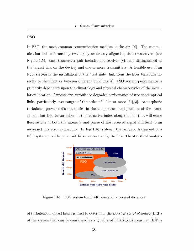
1 – Optical Communications
FSO
In FSO, the most common communication medium is the air [20]. The commu-
nication link is formed by two highly accurately aligned optical transceivers (see
Figure 1.5). Each transceiver pair includes one receiver (visually distinguished as
the largest lens on the device) and one or more transmitters. A feasible use of an
FSO system is the installation of the “last mile” link from the fiber backbone di-
rectly to the client or between di!erent buildings [4]. FSO system performance is
primarily dependent upon the climatology and physical characteristics of the instal-
lation location. Atmospheric turbulence degrades performance of free-space optical
links, particularly over ranges of the order of 1 km or more [21],[3]. Atmospheric
turbulence provokes discontinuities in the temperature and pressure of the atmo-
sphere that lead to variations in the refractive index along the link that will cause
fluctuations in both the intensity and phase of the received signal and lead to an
increased link error probability. In Fig 1.16 is shown the bandwidth demand of a
FSO system, and the potential distances covered by the link. The statistical analysis
Figure 1.16. FSO system bandwidth demand vs covered distances.
of turbulence-induced losses is used to determine the Burst Error Probability (BEP)
of the system that can be considered as a Quality of Link (QoL) measure. BEP is
38

1.2 – Concepts of optical communications
defined in terms of the probability density function of attenuation and is the sum of
three e!ects: beam wander, incidency angle fluctuations, and scintillation. Another
limiting factor for BEP is aerosol scattering. Although rain and snow can hamper
light propagation, the most detrimental environmental conditions for urban FSO
are fog and haze, due to their high concentration of scattering particles with radii
on the same order of magnitude as laser wavelengths. Scattering is the deflection of
incident light from its initial direction, which causes spatial, angular, and temporal
spread, and results in attenuation and distortion of the transmitted signal (on the
order of tens to even hundreds of dB/km), and may drive to the loss of the link.
In general, the scattering phenomenon depends upon the ratio x between particle
size r to radiation wavelength #, according to the following equation:
x =2 · % · r#
(1.10)
When the ratio defined in the above equation is much larger than 1 that is when par-
ticle size r is much larger that radiation wavelength #, as in raindrops and snowflakes
for example, particles do not seriously impede light propagation. Oppositely, parti-
cles that are much smaller than # introduce scattering of the incident waves named
as Rayleigh scattering. This phenomenon produces deviations of light particles and
attenuate incident power according to the 4th power-law of the wavelength. The
worst condition which in fact corresponds to the presence of aerosols is when ratio r
is close to unity and as a consequence scattering is determined by the Mie solution
to the Maxwell wave equation.
In summary, the FSO channel is characterized by three parameters: maximum
BER, maximum atmospherical attenuation used to determine the lost-link condition
as a function of local atmospheric conditions, and the BEP as a measure of link
degradation due to turbulences.
39
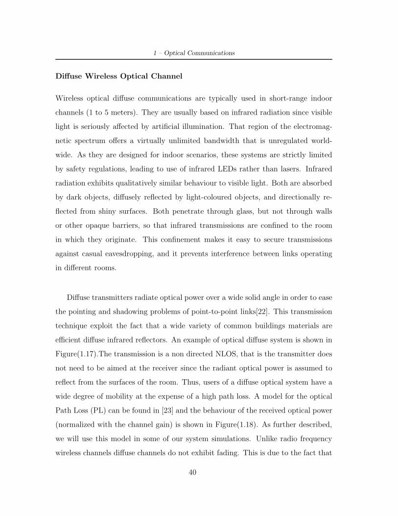
1 – Optical Communications
Di!use Wireless Optical Channel
Wireless optical di!use communications are typically used in short-range indoor
channels (1 to 5 meters). They are usually based on infrared radiation since visible
light is seriously a!ected by artificial illumination. That region of the electromag-
netic spectrum o!ers a virtually unlimited bandwidth that is unregulated world-
wide. As they are designed for indoor scenarios, these systems are strictly limited
by safety regulations, leading to use of infrared LEDs rather than lasers. Infrared
radiation exhibits qualitatively similar behaviour to visible light. Both are absorbed
by dark objects, di!usely reflected by light-coloured objects, and directionally re-
flected from shiny surfaces. Both penetrate through glass, but not through walls
or other opaque barriers, so that infrared transmissions are confined to the room
in which they originate. This confinement makes it easy to secure transmissions
against casual eavesdropping, and it prevents interference between links operating
in di!erent rooms.
Di!use transmitters radiate optical power over a wide solid angle in order to ease
the pointing and shadowing problems of point-to-point links[22]. This transmission
technique exploit the fact that a wide variety of common buildings materials are
e"cient di!use infrared reflectors. An example of optical di!use system is shown in
Figure(1.17).The transmission is a non directed NLOS, that is the transmitter does
not need to be aimed at the receiver since the radiant optical power is assumed to
reflect from the surfaces of the room. Thus, users of a di!use optical system have a
wide degree of mobility at the expense of a high path loss. A model for the optical
Path Loss (PL) can be found in [23] and the behaviour of the received optical power
(normalized with the channel gain) is shown in Figure(1.18). As further described,
we will use this model in some of our system simulations. Unlike radio frequency
wireless channels di!use channels do not exhibit fading. This is due to the fact that
40
1.2 – Concepts of optical communications
Figure 1.17. Example of di!use optical system.
the receive photodiode integrates the optical intensity field over an area of millions
of square wavelengths and hence no change in the channel response is noted if the
photodiode is moved a distance on the order of a wavelength. Thus the large size
of the photodiode relative to the wavelength of light provides a degree of spatial
diversity which eliminates multipath fading. Many channel models based on mea-
surements allow for the accurate simulation of the impulse response of the channel
[24]. Optical indoor channels can be modelled with similar techniques as RF indoor
channels. Besides iterative and statistical approaches, the most proper technique
seems to be ray-tracing combined with models for reflecting surfaces.
Consider a non directed NLOS infrared channel using intensity modulation and
direct detection.As it will shown in the receiver description, the input signal X(t) is
the instantaneous optical power of the emitter, and the output of the channel Y (t)
is the instantaneous current in the receiving photodetector, which is the product
of the photodetector responsivity ) and the integral over the photodetector surface
of the instantaneous optical power at each location. The signal propagates within
a room whose surfaces (e.g. walls, ceiling,..) has reflectivity properties. In the
41

1 – Optical Communications
Figure 1.18. Path Loss of an indoor optical system for both LOS and NLOS cases.
presence of intense infrared and visible background light, which results in additive,
white, nearly Gaussian shot noise n(t) the channel can be modeled as a baseband
system like:
Y (t) = )X(t) & h(t) + n(t) (1.11)
where & denotes the convolution. The channel impulse response of this system
is di!erent from the one characterizing the radio environment because here the
reflection of infrared radiation (and, indeed, visible light) by most surfaces in typical
rooms is predominantly di!use, i.e., the reflected light is scattered into a continuous
distribution of angles, which is nearly independent of the incident angle. Hence,when
a reflecting object is illuminated by the transmitter and this object lies in the receiver
field of view, the result is a pulse extended in time . The temporal dispersion of h(t)
can be expressed by the channel rms delay spread D or by its normalized version
42
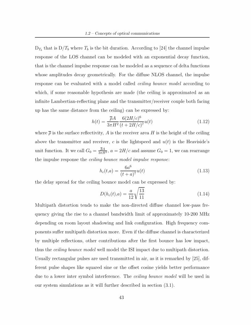
1.2 – Concepts of optical communications
DTbthat is D/Tb where Tb is the bit duration. According to [24] the channel impulse
response of the LOS channel can be modeled with an exponential decay function,
that is the channel impulse response can be modeled as a sequence of delta functions
whose amplitudes decay geometrically. For the di!use NLOS channel, the impulse
response can be evaluated with a model called ceiling bounce model according to
which, if some reasonable hypothesis are made (the ceiling is approximated as an
infinite Lambertian-reflecting plane and the transmitter/receiver couple both facing
up has the same distance from the ceiling) can be expressed by:
h(t) =)A
3%H2
6(2H/c)6
(t + 2H/c)7u(t) (1.12)
where ) is the surface reflectivity, A is the receiver area H is the height of the ceiling
above the transmitter and receiver, c is the lightspeed and u(t) is the Heaviside’s
unit function. It we call G0 = ρA3πH2 , a = 2H/c and assume G0 = 1, we can rearrange
the impulse response the ceiling bounce model impulse response:
hc(t,a) =6a6
(t + a)7u(t) (1.13)
the delay spread for the ceiling bounce model can be expressed by:
D(hc(t),a) =a
12
#13
11(1.14)
Multipath distortion tends to make the non-directed di!use channel low-pass fre-
quency giving the rise to a channel bandwidth limit of approximately 10-200 MHz
depending on room layout shadowing and link configuration. High frequency com-
ponents su!er multipath distortion more. Even if the di!use channel is characterized
by multiple reflections, other contributions after the first bounce has low impact,
thus the ceiling bounce model well model the ISI impact due to multipath distortion.
Usually rectangular pulses are used transmitted in air, as it is remarked by [25], dif-
ferent pulse shapes like squared sine or the o!set cosine yields better performance
due to a lower inter symbol interference. The ceiling bounce model will be used in
our system simulations as it will further described in section (3.1).
43

1 – Optical Communications
Ambient Light Noises
The most commonly encountered ambient light sources are sunlight, skylight, in-
candescent and fluorescent lamps [26],[6],[1]. The optical spectral power densities of
some of them are shown in Figure (1.19). As shown, the spectrum produced by an
electronic-ballast driven fluorescent lamp consists of low and high frequency regions;
the low frequency region resembles the spectrum of a conventional fluorescent lamp
while the high frequency region is attributable to the electronic ballast. In addi-
tion artificial sources emit rapidly fluctuating components associated with higher
harmonics of the mains frequency. These components can reduced by electrical fil-
tering. A deterministic expression that models the interfering signal at the output
Figure 1.19. Optical spectra of common ambient infrared sources scaled tohave the same maximum value.
of the photodiode is in [26]. Noise sources can be organized into these categories:
• Sunlight irradiance produces shot noise in the photodiode that can be con-
sidered as a white Gaussian noise. This noise can be reduced by using tinted
lenses that avoid visible and UV spectral components. Solar irradiation (also
44
1.2 – Concepts of optical communications
called insolation) arrives at Earth at wavelengths determined by the photo-
spheric temperature of the sun (peaking near 5600 ◦C). The main wavelength
interval is between 200 and 3400 nm (0.2 and 3.4 µm), with a maximum power
input close to 480 nm (0.48 µm).
• Artificial lamps (incandescent, halogen and fluorescent) produce shot noise in
the photodiode that can be considered as a narrowband interference. The
e!ect of incandescent or halogen lamps can be seen as a near-dc photocurrent.
On the other hand, fluorescent lamps (especially when driven by electronic
ballast) emit an infrared signal that is periodically modulated at rates of tens
of kHz, and which can severely impair the performance of IR wireless links.
Fluorescent lamps emit strongly at spectral lines of mercury and argon that lie
in the 780-950 nm band of interest for low-cost infrared systems. This e!ect
can be reduced by means of lenses and optical filtering (similar to a bandpass
filter, but designed based on wavelength rather than frequency), or also by
coding and modulation, for example adopting spread spectrum modulation
the artificial light interference behaves like a narrow band jammer, hence its
e!ect reduced thanks to the processing gain advantage of the spread spectrum
technique.
• Thermal noise at receiver has similar nature of any electronic device and is
modelled by the Boltzmann equation.
• Dark current that is a spurious current level produced in the photodiode.
Part of the incident ambient light can blocked by optical filers with a passband
corresponding to the transmitting LED bandwidth, di!erent filters “absorption edge
filters” block only the visible part of the spectrum. A type of filters that is used
in almost all present commercial infrared systems is the “longpass filter”, this can
be thought as a filter that allow to pass all the wavelength beyond wavelength and
45

1 – Optical Communications
are independent of the angle of incidence. The use of longpass filters combined
with silicon p-i-n diodes exhibits a bandpass optical response since the silicon de-
vice does not respond to wavelengths beyond about 1100 nm. In the particular case
of indoor optical communications the interference produced by fluorescent lamps
driven by electronic ballasts causes very large power penalties and the entire ambi-
ent light level varies over several orders of magnitude. Bandpass filters are usually
constructed of multiple thin dielectric layers, these filters can achieve narrow band-
widths, leading to superior ambient light rejection (bandwidths below 1 nm are
available commercially).
1.2.3 Optical Receivers
Optical receivers are transducers capable of transforming optical signals into elec-
trical signals and are called photodetectors. Photodetectors can be classified as
Photodiodes, Phototransistors Photoconductive devices and Photomultiplier tubes.
Photodiodes By far the most common photodetector, a photodiode is a p-n junc-
tion designed to be responsive to optical input.
Phototransistors These are bipolar transistors encased in a transparent case so
that light can reach the Base-Collector diode. The phototransistor works like a
photodiode, but with a much higher sensitivity to light, because the electrons that
tunnel through the Base-Collector diode are amplified by the transistor function.
They are more sensitive than photodiodes but, as their temporal response is much
slower than in a photodiode, their not usually used in optical communications.
Photoconductive devices and Photomultiplier tubes These are high-sensitivity
devices that are far more expensive than photodiodes and phototransistors. They
46

1.2 – Concepts of optical communications
require high bias voltages that make them not practical for optical communications.
The availability of low-cost, low capacitance, large area silicon photodiodes work-
ing in the band of low-cost LED transmitters (that is approximately 780-950nm),
made this reliable optical element used receiver almost in all optical communication
systems. Photodiodes can be used in either zero bias or reverse bias. In zero bias,
light falling on the diode causes a voltage to develop across the device, leading to
a current in the forward bias direction. This is called the photovoltaic effect, and
is the basis for the operation of solar cells (in fact a solar cell can be considered
as a large number of big, cheap photodiodes). Diodes usually have extremely high
resistance when reverse biased. This resistance is reduced when light of an appro-
priate frequency shines on the junction. Hence, a reverse biased diode can be used
as a detector by monitoring the current running through it. The most attractive
characteristics of a photodiode can be summarized as follows:
• High sensitivity at the operating wavelength range (780-950 nm but also 1200-
1600 nm)
• Short response time
• Linearity over a wide range
• Stability with respect to time and temperature
• Low cost and high reliability
Two types of silicon photodiodes are widely available on the market: Ordi-
nary silicon “positive-intrinsic-negative” (PINs) photodiodes and “avalanche photo-
diodes” (APDs). PINs are at present extensively employed in nearly all commercial
infrared links. APDs are essentially p-i-n devices, but operated at a very high reverse
bias, so that photogenerated carriers create secondary carriers by impact ionization,
47

1 – Optical Communications
resulting in internal electrical gain. In principle, this internal gain helps to overcome
receiver amplifier thermal noise, by increasing the receiver SNR when other sources
of noise, that is ambient noise, is weak. When ambient noise is dominant, however,
the random nature of the APD’s internal gain reflects in an increase in the variance
of the shot noise, and as a result the SNR decreases. Other drawbacks are a higher
cost compared to PINs, and temperature-dependent gains. Since our scope is the
simulation of a low-cost system, we will restrict the remaining discussion to ordinary
PINs.
When an incident instantaneous optical power p(t) reach the photodiode surface,
a current is produced in output. This current is called photocurrentand it follows
the expression
i(t) = ) · p(t) (1.15)
where ) is the responsivity and its unit is (A/W). For a typical silicon photodiode
) presents a peak about 950 nm. This responsivity can be estimated from another
parameter: the Quantum Efficiency (Q.E.) (, that is a percentage expressing the
photodiode’s capability to convert light energy to electrical energy. It depends on
the responsivity of the photodiode. Operating under ideal conditions of reflectance,
crystal structure and internal resistance, a high quality silicon photodiode of opti-
mum design would be capable of approaching a Q.E. of 80%.
The risetime of a photodiode it is referred as (tr) and it is the measure of the
photodiode response speed to a stepped light input signal. It is the time required
for the photodiode to increase its output from 10% to 90% of final output level.
Unless a photodiode should be biased on inverse voltage, when applying an excessive
reverse voltage to photodiodes may cause breakdown and severe degradation of
device performance. Thus every photodiode is characterized by a Maximum Reverse
48

1.2 – Concepts of optical communications
Voltage referred as (V r). Any reverse voltage applied must be kept lower than the
maximum rated vale, (V rmax). The photodiode’s Linearity measures the degree
of linearity of the photodiodes output. Generally, when reverse-biased, output is
extremely linear with respect to the illuminance applied to the photodiode junction.
One important parameters of a photodiode is its Junction capacitance that depends
on its area and the bias voltage. This capacitance limits the bandwidth response of
the device, so, unless more active area is needed in order to increase the received
optical power, it penalizes the bandwidth response.
An infrared receiver detects an optical power that is proportional to its e!ec-
tive light-collection area. Increasing the photodiode area is expensive, and tends
to decrease receiver bandwidth and increase receiver noise. Hence, to increase the
e!ective area of the receiver optical concentrators can be deployed. Concentrators
may be of the imaging or non-imaging variety. An example of an imaging concentra-
tor is the telescopes used in long-range, free-space optical links. In the short range
optical communications, non imaging concentrators are chosen.
The e!ective area of a receiver depends on the angle of incidence of the incoming
ray *. If we ignore the reflection losses and consider a photodiode with physical
receiving area A using a concentrator covered with a filter, we have [1]:
Aeff (*) =
$%
&ATs(*)g(*) cos*, 0 " * " %c
0, & > %c
where Ts(*) is the signal transmission of the filter (if the source bandwidth is not nar-
row this can be considered an average of the filter transmission over di!erent wave-
lengths and/or over di!erent angles of incidence if di!erent ray strike are present),
g(*) is the concentrator gain, %c is the concentrator FOV (semiangle). Usually
%c " %/2. Non imaging concentrators exhibit a trade-o! between gain and FOV.
In the particular case of non direct optical communication, hemispherical lens are
the most suitable due to the very large FOV (%c ' %/2 and gain g(*) ' n2).
49

1 – Optical Communications
In Figure(1.20) an example of two di!erent hemispherical concentrators is shown.
When a longpass filter is is employed, a planar longpass filter can be placed between
the hemisphere and the detector. When bandpass filtering is utilized, it is not de-
sirable to employ a planar filter in the configuration shown in Figure(1.20-a). As *,
the angle from which rays are received, shifts, so does &, the angle at which light
strikes the filter. This shifts the filter passband, decreasing the filter transmission
Ts(*) for some *. Instead, as shown in Figure(1.20-b), the bandpass filter should
be deposited or bonded onto the outer surface of the hemispherical concentrator.
In this case rays that reach the detector are incident upon the filter at small values
of the angle & independently of the angle *, thus minimizing the shift of the filter
passband, and maximizing its transmission. Di!erent types of concentrators that
privilege the gain respect to the FOV are suitable for di!erent types of systems.
Figure 1.20. Example of two di!erent non-imaging hemispherical optical concen-trators: a) with a planar filter and b) with and hemispherical filter.
50
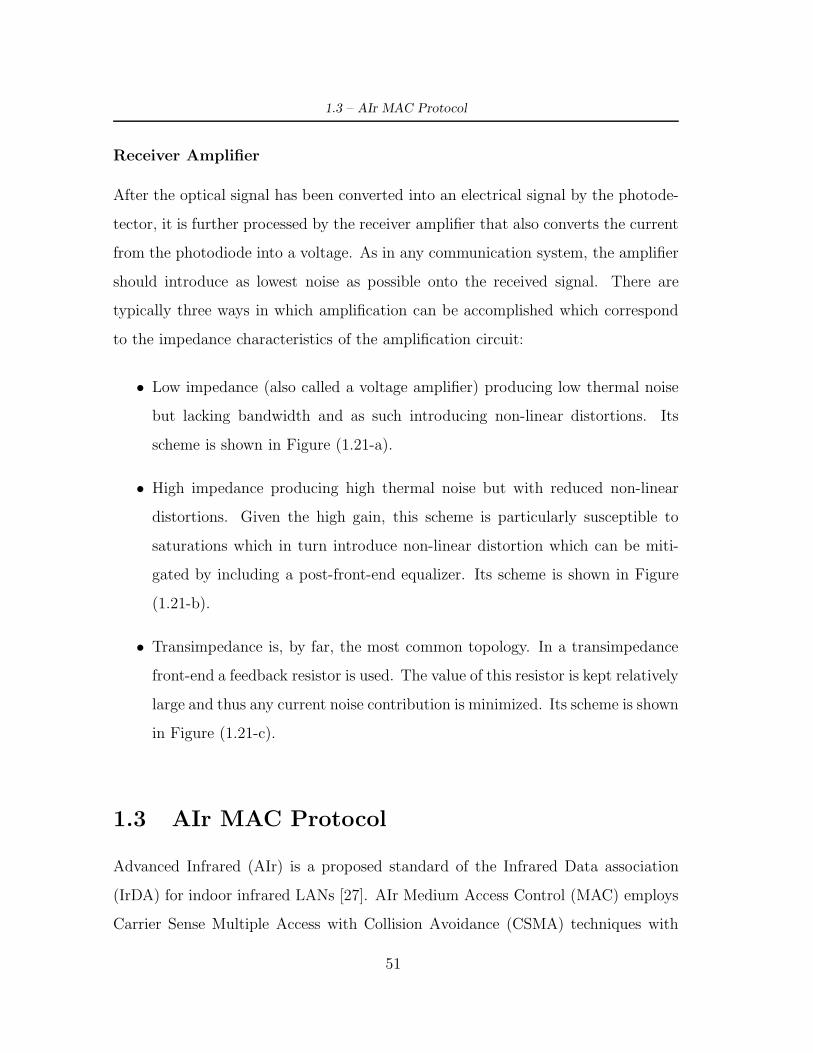
1.3 – AIr MAC Protocol
Receiver Amplifier
After the optical signal has been converted into an electrical signal by the photode-
tector, it is further processed by the receiver amplifier that also converts the current
from the photodiode into a voltage. As in any communication system, the amplifier
should introduce as lowest noise as possible onto the received signal. There are
typically three ways in which amplification can be accomplished which correspond
to the impedance characteristics of the amplification circuit:
• Low impedance (also called a voltage amplifier) producing low thermal noise
but lacking bandwidth and as such introducing non-linear distortions. Its
scheme is shown in Figure (1.21-a).
• High impedance producing high thermal noise but with reduced non-linear
distortions. Given the high gain, this scheme is particularly susceptible to
saturations which in turn introduce non-linear distortion which can be miti-
gated by including a post-front-end equalizer. Its scheme is shown in Figure
(1.21-b).
• Transimpedance is, by far, the most common topology. In a transimpedance
front-end a feedback resistor is used. The value of this resistor is kept relatively
large and thus any current noise contribution is minimized. Its scheme is shown
in Figure (1.21-c).
1.3 AIr MAC Protocol
Advanced Infrared (AIr) is a proposed standard of the Infrared Data association
(IrDA) for indoor infrared LANs [27]. AIr Medium Access Control (MAC) employs
Carrier Sense Multiple Access with Collision Avoidance (CSMA) techniques with
51
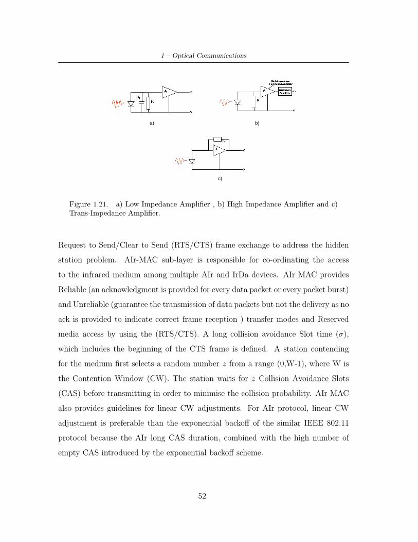
1 – Optical Communications
a) b)
c)
Figure 1.21. a) Low Impedance Amplifier , b) High Impedance Amplifier and c)Trans-Impedance Amplifier.
Request to Send/Clear to Send (RTS/CTS) frame exchange to address the hidden
station problem. AIr-MAC sub-layer is responsible for co-ordinating the access
to the infrared medium among multiple AIr and IrDa devices. AIr MAC provides
Reliable (an acknowledgment is provided for every data packet or every packet burst)
and Unreliable (guarantee the transmission of data packets but not the delivery as no
ack is provided to indicate correct frame reception ) transfer modes and Reserved
media access by using the (RTS/CTS). A long collision avoidance Slot time (+),
which includes the beginning of the CTS frame is defined. A station contending
for the medium first selects a random number z from a range (0,W-1), where W is
the Contention Window (CW). The station waits for z Collision Avoidance Slots
(CAS) before transmitting in order to minimise the collision probability. AIr MAC
also provides guidelines for linear CW adjustments. For AIr protocol, linear CW
adjustment is preferable than the exponential backo! of the similar IEEE 802.11
protocol because the AIr long CAS duration, combined with the high number of
empty CAS introduced by the exponential backo! scheme.
52

Chapter 2
Ultra-wide band communications
2.1 Historical Overview & State of the Art
Ultra-wideband (UWB) is an emerging wireless technology, and has been considered
as one of the promising technologies to provide multimedia services in both indoor
and outdoor applications.The UWB transmission technique is characterized by an
instantaneous spectral occupancy in excess of 500 MHz or fractional bandwidth of
more than 20%. With the benefits of high data rate, low power spectral density, ca-
pability to capture multipath energy, and ability of accurate positioning, UWB has
demonstrated its potential in future multimedia applications as well as in industrial
control and maintenance medical monitoring, radar imaging, home automation, etc.
A breakpoint in the history of UWB was when the Federal Communication
Commission (FCC) allowed spontaneous UWB indoor and outdoor transmissions
between the band from 3.1 to 10.6 GHz on an unlicensed basis [28].
This chapter begins discussing the state-of-the art of UWB and then continues
by providing a theoretical framework of UWB radio communications, modulation
53

2 – Ultra-wide band communications
techniques and Power Density Spectra. Since this thesis focuses on the convergence
between optical and UWB systems, common aspects between this two transmission
techniques will be highlighted (i.e pulse signals and pulse based modulations like
PPM and OOK.
Despite its renewed interest during the past decade, UWB has a history as long
as radio. In Guglielmo Marconi’s experiments over a century ago radio communi-
cations utilized enormous bandwidth as information was indeed conveyed through
a spark-gap transmitter to transmit the Morse Code over the air. Nevertheless
technological limitations (spark-gap transmitters were noisy and ine"cient) and
commercial pressure for more reliable communications strongly favoured, however a
shift of research and development towards continuous-wave transmissions. During
the World War II pulse transmissions techniques were adopted for security reasons
in for military transmissions. Since pulse-based systems were able to guarantee
higher ranges compared to continuous transmissions, the former started to be con-
sidered also for civilian applications. In fact these systems allowed to regenerate the
pulses, thus to avoiding the accumulation of distortion from noise and other system
imperfections. Moreover despite being analog, pulse-modulated systems permitted
the multiplexing of communication channels on the time division basis. During the
1960s, thanks to high sensitivity to scatters and low power consumption UWB tech-
nology was introduced in the radar systems with the works of Harmuth [29], Ross
[30] and others [31]. In 1977 the USAF started a research program on IR systems
that lasted until 1989. It was in 1989 that the U.S. Department of Defense (DoD)
coined the term “ultra wideband” for devices occupying at least 1.5 GHz, or a -20
dB fractional bandwidth exceeding 25% [32].
Modern history of Ultra Wideband starts o"cially in 2002, when the Federal
54

2.1 – Historical Overview & State of the Art
Communication Commission (FCC) allowed spontaneous emission of UWB signals
among the huge range of frequencies (3.6-10.1GHz) at the noise floor [28]. FCC
proposal allowed the coexistence of RF systems and UWB radios, these latter being
able to operate using low-power ultra-short information bearing pulses. Since the
FCC regulations were released, several research institutions, industry and govern-
ment agencies undertook e!orts to asses and exploit the potential of UWB radios:
examples are short-range very high-speed broadband access to the Internet, cable
replacement, very accurate (centimeter-level) localization, high resolution ground-
penetrating radar, through-wall imaging and many others.
The most common definition of the term Ultra Wideband comes from the UWB
radar world and refers to electromagnetic waveforms that are characterized by an
instantaneous fractional energy bandwidth greater than about 20! 25%. UWB sig-
nals are very often characterized by the transmission of pulses with a short duration
in time (in the order of ns), in this case considering the duration of one pulse, the
instantaneous energy must be computed over this interval. However the FCC regu-
lations leave open the possibility of producing UWB signals also with nonimpulsive
schemes. In this work however we will focus on Impulse Radio UWB. One source
bit can be represented with a single pulse, but commonly a single bit of information
involves the processing of several pulses, and in this case the energy bandwidth (that
is the energy in the frequency interval (fH ! fL) is referred to the group of pulses.
If more pulses per bit are considered, a well-based definition of useful signal energy
must be provided. According to FCC, the Energy Spectral Density (ESD) lower and
upper frequencies must be considered at !10dB. Thus since fractional bandwidth is
defined as'
fH−fL
fc
(, where fc is the central frequency, a systems with fc ( 2.5GHz
need to have a !10dB bandwidth of at least 500MHz [33].
55

2 – Ultra-wide band communications
If fL is the lower limit of the Energy Spectral Density (ESD) and fH is the
higher limit, then the center frequency of the spectrum is located at'
fH+fL
2
(and
the fractional bandwidth is defined as the ratio of the energy bandwidth and the
center frequency:
fb ='fH ! fL
fH+fL
2
((2.1)
For wireless communications the FCC power level regulations are very low (below
-41.3 dBm), this power constraint allows UWB to coexist with already available
legacy systems such as global positioning system (GPS) and the IEEE 802.11 wire-
less local area networks (WLANs) within the band 3.6-10.1GHz.
Provided that UWB signal power is forced to be at the noise floor, UWB signals
are very di"cult to intercept by eavesdroppers and are particularly secure against
jamming (AntiJamming capability AJ). These characteristics are typical of spread
spectrum schemes that have been recently proposed, for both wireless and wired
communications systems, as a way for reducing the e!ect of jamming and multipath
dispersion.
2.2 Principles of Impulse Radio in UWB commu-
nications
As previously mentioned the most common and traditional way of emitting an UWB
signal is by radiating pulses that are very short in time. This transmission tech-
nique goes under the name of Impulse Radio (IR). The way by which the information
data symbols modulate the pulses may vary, for example Pulse Position Modulation
(PPM), Pulse Amplitude Modulation (PAM) and On O! Keying (OOK) are possible
schemes. In addition to modulation and in order to shape the spectrum of the gen-
erated signal, the data symbols are encoded using pseudo-random or pseudo-noise
56

2.2 – Principles of Impulse Radio in UWB communications
(PN) codes. In a common approach, the encoded data symbols introduce a time
dither on generated pulses leading to the so called Time-Hopping UWB (TH-UWB).
Direct-Sequence Spread Spectrum (DS-SS), that is amplitude modulation of basic
pulses by encoded data symbols, in the IR version indicated as Direct-Sequence
UWB (DS-UWB), also seems particularly attractive. RF modulation is rarely men-
tioned in conjunction with UWB systems, which typically operate in the base-band.
While RF modulation is obviously applicable to UWB as well, a shift in operating
frequency can be potentially obtained by pulse shaping.
In Figure 2.1 a simple M-ary TH-UWB transmission chain is provided. Given the
binary sequence to transmit b=(..,b0,b1,..,bk,bk+1,..), generated at a rate of Rb = 1Tb
bits/s, a first system repeats each bit Ns times and generates a binary sequence
(..,b0,b0,..,b0,b1,b1,..,b1,bk,bk,..,bk,bk+1,bk+1,..,bk+1,..)=(..,a0,a1,..,aj ,aj+1,..)=a at the rate
Rcb = NsTb
= 1Ts
. This system introduces redundancy and is a (Ns,1) block coder in-
dicated as a code repetition coder. In the classical terminology this is a channel
coder. A second block called transmission coder applies an integer-valued code
c=(..,c0,c1,..,cj,cj+1,..) to the binary sequence a and generates a new sequence d.
The generic element of this sequence d is expressed as follows:
dj = cjTc + aj" (2.2)
where Tc is a time constant that is called “chip time” or “chip distance” and " is the
PPM time shift. Since bit time Tb is divided into Ns time slots each with duration
of Ts seconds, and each Ts must contain the chip time and the time shift, for all cj
the time constraint cjTc < Ts must be provided and this is also true that " < Tc.
The code c is a integer-valued code that can be pseudo-random. If we consider it
as a pseudo-random code, its generic element cj satisfies 0 " cj " Nh ! 1 where
Nh is the code cardinality. The code c can be periodic, and in this case, its period
is indicated by Np. In the most commonly adopted case the code period is chosen
57

2 – Ultra-wide band communications
BINARY SOURCE
CODEREPETITION
CODER(Ns,1)
TRANSM.CODER
PPMMODULATOR
PULSE SHAPER
p(t)
(bit/s) (bit/s) (symbols/s)
s(t)
(pulses/s)
Figure 2.1. Transmission scheme for a PPM-TH-UWB.
equal to the length of the repetition code, this choice has clear e!ect on the PSD of
the transmitted signal [34]. In the presented scheme the transmission coder plays a
double role of code division multiple access coder and of spread spectrum shaper of
the transmitted signal. The real-valued sequence d enters a third system, the PPM
modulator, which generates a sequence of unit pulses (Dirac pulses ,(t)) at a rate
of RpNsTb
= 1Ts
pulses per second. These pulses are located at times jTs + dj, and
therefore shifted in time from nominal positions jTs by dj. Pulses occur at times
(jTs + cjTc + aj"). Note that code c introduces a TH shift on the generated signal,
and it is for this reason that is indicated as TH code. The shift introduced by the
PPM modulator, aj", is usually much smaller than the shift introduced by the TH
code, cjTc, that is aj" " cjTc, except for cj = 0. The last block in the scheme is
the pulse shaper filter with impulse response p(t). The impulse response p(t) must
be such that the signal at the output of the pulse shaper filter is a sequence of
strictly non-overlapping pulses. The choice of p(t) is crucial since it a!ects the PSD
of the transmitted signal [34]. The TH-UWB transmitted signal can be expressed
as follows:
s(t) =∞"
j=−∞
p(t ! jTs ! cjTc ! aj") (2.3)
The generated pulse must be in the order of nanoseconds: this is possible after the
introduction of UWB Large Current Radiator (LCR) introduced by Harmuth (1990).
58

2.2 – Principles of Impulse Radio in UWB communications
The LCR is current driven, and the antenna radiates a power that is proportional to
the square of the derivative of current. When a step function current, for example,
is applied to the antenna, a pulse is generated: the steeper the step function current,
the narrower the generated pulse. A pulse shape that can be generated in the easiest
way by pulse generator has the gaussian shape, and it is described by the following
p(t) = ± 1)2%+2
e−)
t2
2!2
*= ±
)2
!e−
)2"t2
#2
*(2.4)
where !2 = 4%+2 is called shape factor and +2 is the variance. To be radiated in
an e"cient way, however, a basic feature of the pulse is to have a zero dc (direct
current) o!set. Several pulse waveform can be considered, provided that this con-
dition is verified. Gaussian derivatives are suitable, and in particular the second
order derivative is the most commonly adopted. In Impulse Radio is possible to
shape the spectrum by changing the pulse waveform: basically the spectrum may
be shaped in three di!erent ways, i.e. pulse width variations, pulse di!erentiation
and a combination of base functions. The Gaussian pulse used in practice must be
truncated to a desired time duration because provided that the pulse is infinite in
time ISI between pulses would be unavoidable. In Figure 2.2 is shown an example
of a TH-2PPM-UWB transmitted signal. In particular two bits are considered with
a repetition coder with length Ns=5.
2.2.1 Power Spectral Density of IR-TH-PPM UWB signal
The Power Spectral Density (PSD) of a TH-PPM UWB signal is reported. Based
on the similarities of the signal format 2.3 and the output of an analog PPM mod-
ulator consisting of a train of identically shaped and strictly non-overlapping pulses
the PSD of a TH-PPM signal was evaluated in [35]. Here the authors show how
the PPM signal can be considered modulated by a periodic signal and therefore
is reasonable for the PSD to be discrete and have frequency components at the
59

2 – Ultra-wide band communications
0 0.5 1 1.5 2 2.5 3x 10⁻⁸
−2
0
2
4
6
8x 10⁻³
Time [s]
Ampl
itude
[V]
TH−PPM UWB transmitted signal
Figure 2.2. Example of UWB TH-PPM transmitted signal with Ns=5, av-erage transmitted power=-30dB, Ts=3ns, Tc=1ns, Nh=3, Np=5, Tm=0.5ns,!=0.25ns and "=0.5ns.
fundamental. As reported also in [34], the fundamental frequency that influences
the PSD shape depends on the period of the code (Np), that is the fundamental is
fp = 1/Tp = 1/(NpTs), where Ts is the pulse interval of the system. Must be noted
that the pulse repetition frequency 1/Ts = Np/Tp is a multiple of the fundamental
frequency of the periodic waveform; therefore, the PSD is composed of lines occur-
ring at 1/Tb and its armonics. If, as common in practice, Np is set equal to Ns, that
is, the periodicity of the code coincides with the number of pulses per bit, spectrum
lines occur at 1/Tb and its armonics, where Tb = NsTs = NpTs is the bit interval.
Provided that the source b is a strict-sense stationary discrete random process,
and the di!erent extracted variables bk are statistically independent with a common
probability density function w, then the PSD of a TH-PPM UWB signal with Np =
Ns can be expressed by:
Ps(f) =|Pν(f)|2
Tb
+1 ! |W (f)|2 +
|W (f)|2
Tb
+∞"
n=−∞
,'f ! n
Tb
(,(2.5)
60

2.2 – Principles of Impulse Radio in UWB communications
where Pν(f) is the Fourier transform of a signal $(t) called “multi-pulse”, that is a
signal that takes count of all the Ns pulses that are used for the transmission of a
single bit. The TH-PPM signal can be imagined as sequence of multi-pulse signal.
If we define the single multi-pulse signal as:
$(t) =Ns"
j=1
p(t ! jTs ! (j) (2.6)
where (j is the the time shift due to the TH code, its Fourier transform can be
expressed by:
Pν(f) = P (f)Ns"
m=1
e−j(2πf(mTs+ηm)) (2.7)
The term |W (f)|2 that is the weight value of the spectral lines, depends on the
statistical properties of the source. An example of the Power Spectral Density of
a TH-PPM UWB signal is shown in Figure(2.3). The provided spectrum shape is
−8 −6 −4 −2 0 2 4 6 8x 10⁹
0
0.2
0.4
0.6
0.8
1
1.2
1.4
1.6
1.8
2x 10⁻¹⁵
Frequency [Hz]
Powe
r Spe
ctra
l Den
sity
[V2 /H
z]
Figure 2.3. PSD of an IR-TH-PPM UWB signal.
strictly dependent on the used TH code: in fact the e!ect of the code in fact is to
whiten the spectrum since power distributes over a larger number of spectrum lines
and spectral peaks are less accentuated.
61

2 – Ultra-wide band communications
2.2.2 Emission masks
UWB radio signals must coexist with other radio signals. Possible interference from
and onto other communications systems must be contained within regulated values
that indicate the maximum tolerable power be present in the air interface at any
given frequency. For this reason in 2002 FCC released 2 di!erent emission masks.
Mainly 3 types of UWB devices were defined, Imaging Systems, Communication
and Measurement Systems and Vehicular radar, thus both the outdoor and the
indoor channels must be considered. Emission masks impose power limitations on
the e!ective radiated power and di!erences between outdoor and indoor masks are
more stringent power constraints for the outdoor environment in the band between
1.99-3.1GHz and above 10.6GHz. The e!ective radiated power is the E!ective
109 1010
−75
−70
−65
−60
−55
−50
−45
−40
Frequency [MHz]
PSD
[dBm
/MHz
]
FCC UWB indoor emission mask
Figure 2.4. FCC indoor emission mask for UWB devices (FCC,2002).
Isotropic Radiated Power (EIRP) for a given range of operating frequencies, and
is given by the product of available power of the transmitter PTX , which is the
maximum power that the transmitter can transfer to the transmitter antenna and
62
2.2 – Principles of Impulse Radio in UWB communications
109 1010
−75
−70
−65
−60
−55
−50
−45
−40FCC UWB outdoor emission mask
Frequency [MHz]
PSD
[dBm
/MHz
]
Figure 2.5. FCC outdoor emission mask for UWB devices (FCC,2002).
the gain of the transmitter antenna GAT .
EIRP = PTX · GAT (2.8)
As seen in Figures 2.4,2.5 EIRP is measured in dBm, that is 10 log10(EIRPmWatts).
The available power of the transmitter PTX is e!ectively transferred from the trans-
mitter to the antenna when the condition for maximum power transfer between
the output impedance of the transmitter ZoTX and the input impedance of the an-
tenna ZAT is verified, ZAT = Z∗oTX . An equivalent way of ruling emitted radiations
is to impose limits on the field strength VS in V/m. VS represents the voltage one
should apply to the characteristic impedance of free-space ZFS to obtain an available
power PTX after propagation over a distance D. ZFS is 120% that is approximately
377 & and in principle it is independent of the frequency. The relation between field
strength and available power is
EIRP *=V 2
S
3774%D2 (2.9)
63
2 – Ultra-wide band communications
the power defined in (2.8) is an average power, that is, the ratio of the transmitted
energy per bit Eb over the bit period Tb. In a binary IR scheme, given the energy
of a single pulse Ep, PTX is thus expressed by:
PTX =NsEp
Tb=
NsEp
NsTs=
Ep
Ts(2.10)
where 1/Ts is the pulse repetition rate. As shown in (2.10), di!erent IR signals can
exhibit the same PTX with di!erent pulse energy Ep depending on the repetition
rate. At equal average power, signals with low repetition rate may have higher Ep.
For equal pulse duration, this is equivalent to saying that the maximum instanta-
neous power may be markedly di!erent among signals with similar average power.
Emission masks impose limits on the PSD of emitted signals, that is on EIRP spec-
tral density, expressed for example in dBm/Hz or dBm/MHz. Emission masks are,
however commonly provided in terms of power value at a given frequency, rather
than power density values. The values of the mission masks at a given frequency fc
indicates , the maximum allowed EIRP within a measured bandwidth (mb) centered
around fc. For signals having bandwidth B =mb, the maximum allowed EIRP value
is exactly the value of EIRPmb. For a signal having bandwidth B ( mb, the maxi-
mum allowed EIRP is equal to the sum of the EIRPmb values that are provided by
the mask corresponding to the frequency range occupied by the signal. In particular
we can express a formal definition of EIRPmb for a signal having B=mb as:
EIRPmbB
mb= EIRP + V 2
3774%D2 (2.11)
Regarding indoor and outdoor UWB systems , the masks limits operation to a -10
dB bandwidth lying between 3.1 and 10.6 GHz, and sets very stringent limits on
out-of-band emission masks. The emission masks values of the FCC are reported in
tables (2.2.2) and (2.2.2), the rule also specifies a limit on the peak level of emission
within a band of 50 MHz bandwidth centered on the frequency fM , at which the
highest radiated emission occurs. The limit is set to 0 dBm/50MHz, that is, the
64

2.2 – Principles of Impulse Radio in UWB communications
power computed over a frequency range of 50 MHz around fM is limited to 0 dBm.
Frequency in MHz EIRPmb in dBm
0-960 -41.3960-1610 -75.31610-1990 -53.31990-3100 -51.33100-10600 -41.3
Above 10600 -51.3
Table 2.1. Average Power Limits set by FCC in the U.S. for Indoor UWB Devices.
Frequency in MHz EIRPmb in dBm
0-960 -41.3960-1610 -75.31610-1990 -63.31990-3100 -61.33100-10600 -41.3
Above 10600 -61.3
Table 2.2. Average Power Limits set by FCC in the U.S. for Outdoor UWB Devices.
In february 2007 the European Community produced a document “on allowing the
use of the radio spectrum for equipment using ultra-wideband technology
in a harmonised manner in the Community”. Specifically the EC has chosen
to make use of only part of the spectrum that was approved for use in the US in
2002. In Europe UWB communications Part 15 limit of -41.3 dBm/MHz will be
applied over the 6.0- to 8.5-GHz frequency range, whereas in the United States the
FCC applies this over a broader spectrum from a much lower frequency. It is also
applied provisionally until the end of 2010 in the 4.2 to 4.8-GHz range (see table
2.2.2).
65
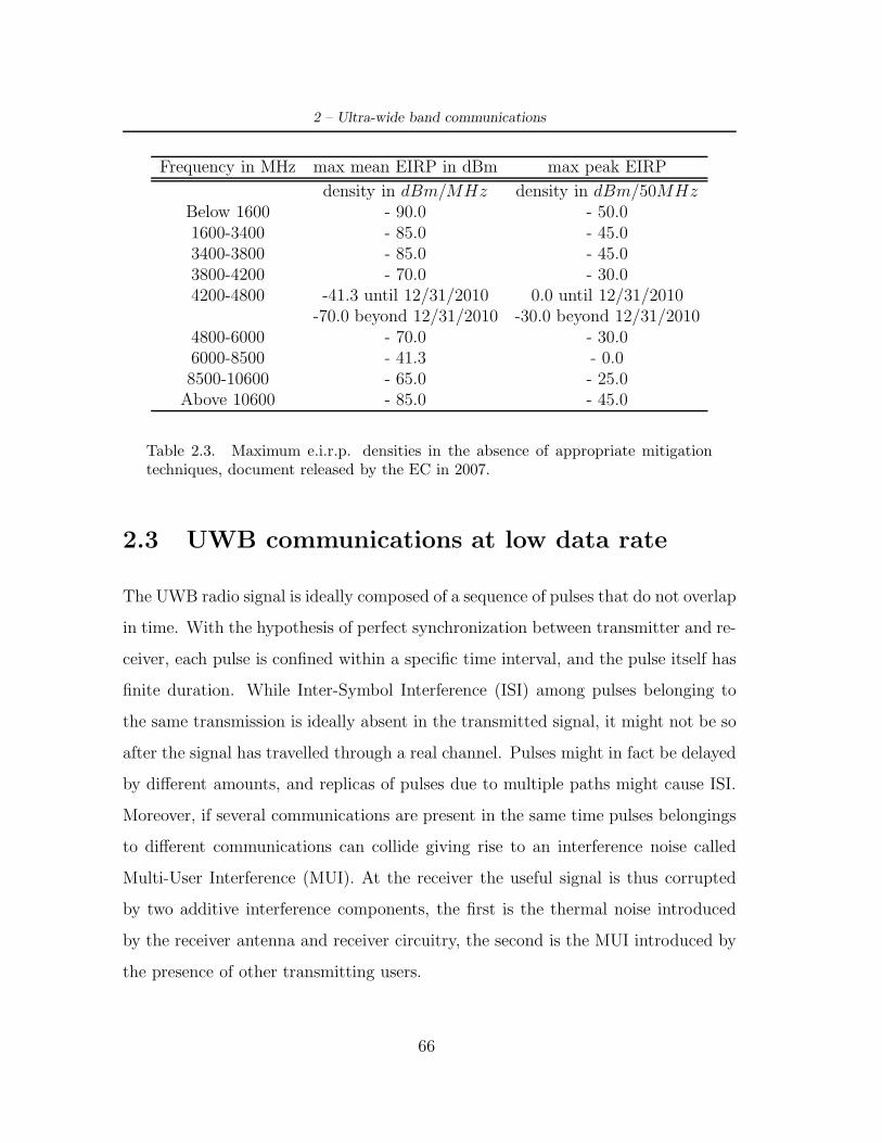
2 – Ultra-wide band communications
Frequency in MHz max mean EIRP in dBm max peak EIRP
density in dBm/MHz density in dBm/50MHzBelow 1600 - 90.0 - 50.01600-3400 - 85.0 - 45.03400-3800 - 85.0 - 45.03800-4200 - 70.0 - 30.04200-4800 -41.3 until 12/31/2010 0.0 until 12/31/2010
-70.0 beyond 12/31/2010 -30.0 beyond 12/31/20104800-6000 - 70.0 - 30.06000-8500 - 41.3 - 0.08500-10600 - 65.0 - 25.0
Above 10600 - 85.0 - 45.0
Table 2.3. Maximum e.i.r.p. densities in the absence of appropriate mitigationtechniques, document released by the EC in 2007.
2.3 UWB communications at low data rate
The UWB radio signal is ideally composed of a sequence of pulses that do not overlap
in time. With the hypothesis of perfect synchronization between transmitter and re-
ceiver, each pulse is confined within a specific time interval, and the pulse itself has
finite duration. While Inter-Symbol Interference (ISI) among pulses belonging to
the same transmission is ideally absent in the transmitted signal, it might not be so
after the signal has travelled through a real channel. Pulses might in fact be delayed
by di!erent amounts, and replicas of pulses due to multiple paths might cause ISI.
Moreover, if several communications are present in the same time pulses belongings
to di!erent communications can collide giving rise to an interference noise called
Multi-User Interference (MUI). At the receiver the useful signal is thus corrupted
by two additive interference components, the first is the thermal noise introduced
by the receiver antenna and receiver circuitry, the second is the MUI introduced by
the presence of other transmitting users.
66

2.3 – UWB communications at low data rate
2.3.1 Multi User Interference (MUI)
In this section the MUI problem for multi-access impulse radio UWB (IR-UWB)
systems is considered. Since the number of interferers is unknown a priori, a typical
assumption that can be made is to consider the multiuser interference as a Gaussian
distributed process, this approximation is referred as the Standard Gaussian Ap-
proximation (SGA). The SGA relies on the observation that when MUI is provoked
by the sum of a large number of users, interference can be treated as an additive
Gaussian noise with uniform power spectrum over the frequency band of interest.
Under this assumption, receiver tolerance to MUI easily expresses as a function of
the average signal to noise ratio at the reference receiver, where noise power is cal-
culated as the sum of thermal noise and average MUI powers. The SGA has two
main advantages over the other proposed models (see [36] for a complete survey), it
is simple, i.e., few system parameters are required for evaluating performance and it
is fast, i.e., the average BER is provided through an explicit form which can be cal-
culated at a reduced computational cost. The SGA however, is based on the central
limit theorem, and provides thus accurate BER estimations only for scenarios with
high MUI levels, i.e., for densely populated networks. Provided that the intended
scenario comprises only few nodes, the SGA may provide a BER estimations that is
optimistic if compared with the theoretical value. In the following the SGA model
is briefly described because most of the attention will be focused on a di!erent MUI
model, the Pulse Collision Model [36]. Based on the Pulse Collision Model, will be
described in section 2.5 the UWB2 MAC protocol that is used in our simulations.
The Standard Gaussian Approximation
Consider the TH-UWB signal expressed by equation (2.3), from this expression, if
we consider that each user is assigned a di!erent TH code, the transmitted signal
67
2 – Ultra-wide band communications
is:
sTX(t) =-
ETX
∞"
j=−∞
p0(t ! jTs ! cjTc ! "a%j/Ns&) (2.12)
where p0(t) is the energy-normalized waveform of the transmitted pulses, ETX is
the energy of each pulse, Ts is the average pulse repetition period, 0 " cjTc " Ts is
the time shift of the jth pulse provoked by the TH code, " is the PPM shift, ax is
the xth bit (that is a iid variable) of a, Ns is the number of pulses transmitted for
each bit, and ,x- is the inferior integer part of x. If the channel model is assumed
a general flat AWGN model, and perfect synchronization between transmitter TX
and receiver RX is assumed, the channel output is corrupted by thermal noise and
MUI generated by Ni interfering IR-UWB devices. The received signal thus writes:
sRX(t) = ru(t) + rmui(t) + n(t) (2.13)
where ru(t), rmui(t) and n(t) are the useful signal, MUI, and thermal noise, respec-
tively. As regards ru(t), one has:
ru(t) =-
Eu
∞"
j=−∞
p0(t ! jTs ! cjTc ! "a%j/Ns& ! -) (2.14)
where Eu = !2ETX and - is the propagation delay of the channel (that is known
at receiver due to the perfect synchronization hypothesis). as regard rmui(t), we
assume that all interfering signals are characterized by same Ts but not the same
Ns, and thus:
rmui(t) =Ni"
n=1
)E(n) ·
∞"
j=−∞
p0(t ! jTs ! c(n)j Tc ! "a(n)
%j/N(n)s &
! - (n)) (2.15)
where E(n) and - (n) are received energy per pulse and delay for the nth interfering
user. The relative delay '- (n) = - ! - (n) is assumed to be a random variable
uniformly distributed between 0 and Ts. Both TH codes and data bit sequences are
randomly generated and correspond to pseudo-noise sequences, that is, c(n)j terms
68

2.3 – UWB communications at low data rate
are assumed to be independent random variables uniformly distributed in the range
[0,Ts), and a(n)x values are assumed to be independent random variables with equal
probability to be “0” or “1”. Finally, signal n(t) in (2.13) is Gaussian noise, with
double-sided power spectral density N0/2.
If a coherent correlator followed by a ML detector is the considered receiver. We
have that in each bit period (that is Tb = NsTs seconds), the correlator converts
the received signal of (2.13) into a decision variable Z, which forms the input of the
detector. Here Soft is performed, i.e., the signal formed by Ns pulses is considered
as a single multi-pulse signal. The received signal is thus cross-correlated with a
correlation mask m(t) that is matched with the train of pulses representing one bit.
The input of the detector Z(x), for a generic bit ax, can be thus expressed as follows
by the sum of three components:
Z(x) = Zu + Zmui + Zn (2.16)
that are the useful term, the MUI term and the Gaussian noise term, respec-
tively.The bit estimation exploited in the receiver is based on the comparison of
the Z(x) value with a predefined zero-valued threshold according to the following
rule: if Z(x)¿0 decision is “0”, decision is “1” otherwise. For independent and
equiprobable transmitted bits, the average BER at the output of the detector is:
BER =1
2Prob(Z(x) < 0|ax = 0)+
1
2Prob(Z(x) > 0|ax = 1) = Prob(Z(x) < 0|ax = 0)
(2.17)
More specifically, all this terms depend on the transmitted pulse waveform p0(t). In
particular if we consider its autocorrelation function R0(t):
R0(t) =
. +∞
−∞p0(.)p0(. ! t)d.
and we define the term '(") = 1 ! R0("), we have that Zn, the Gaussian term has
zero mean and variance +2n = NsN0'("). Under the SGA also the term Zmui is
69
2 – Ultra-wide band communications
modeled as Gaussian random variable, and its variance that can be be interpreted
as the MUI power at the correlator output at the average operating conditions. Like
Zn, also Zmui depends on the waveform p0(t), and if we define the term +2M as:
+2M =
. +∞
−∞
'. +∞
−∞p0(t ! -)(p0(t) ! p0(t ! ")dt)
(2d-
we can write the variance of the MUI term as:
+2mui =
Ns
Ts+2
M
Ni"
n=1
En (2.18)
The useful component of the decision variable is Zu that can be expressed like:
Zu =
$%
&+Ns
)Eu'("), if ax = 0
!Ns
)Eu'("), if ax = 1
Under the SGA, therefore, the average Bit Error Rate (BER) writes:
BER =1
2erfc
/01121
2
/'NsEu'(")
N0
(−1
+' NsTs'(")
+2M
3Nin=1(E
(n)/Eu)
(−14−14
The SGA is derived from the central limit theorem and is thus valid only asymptot-
ically.
The Pulse Collision Model
We will firstly briefly introduce the pulse collision model basics as reported in [2],
and subsequently describe the model more deeply as can be found in [36]. The
time occupied by one single UWB pulse indicated by Tm is defined here as the time
interval typically centered on the main lobe in which most of the energy of the pulse
at the receiver is concentrated. Typical values for Tm lie between 70 psecs and 20
nsecs depending upon transmitted pulse shape and channel behaviour. Since no
synchronization between users is provided, is reasonable to assume that the inter-
arrival time of di!erent packets follows a Poisson distribution. Each packet contains
70

2.3 – UWB communications at low data rate
a set of pulses, each subset of Ns pulses carrying the information of one bit. The
pulse inter-arrival process is a complex phenomenon that depends on modulation,
dithering, codes and so on. To try to express the probability of pulse collision in a
closed form, let us assume that the pulse inter-arrival process is a Poisson process
itself. Therefore the probability that one or more pulses collide with the useful pulse
when PU packets are transmitted over the air interface by NU active users can be
compared to the Aloha collision probability when the information unit is the pulse
instead of the packet. This probability can be expressed as:
ProbPulseCollision = 1 ! e(−2·(PU−1)·TmTs
) (2.19)
where Ts is the average pulse repetition period. The number of transmitted packets
PU depends on the number of active users NU , and if L is the packet length, Rb is
the data rate (that is 1/(Ns · Ts), where Ns is the number of transmitted pulses per
bit) and G is the packet generation rate, its instantaneous value is:
PU =NU · L · G
Rb(2.20)
Assuming that a pulse collision causes a random decision at the receiver the pulse
error probability can be expressed as:
ProbPulseError = 0.5 · ProbPulseCollision (2.21)
Considering that each bit is encoded into NS pulses we assume an error on the bit
when more than Ns/2 pulse errors occur. This corresponds to assuming a hard
receiver detection. Bit error probability is thus expressed by:
ProbBitError =Ns"
i='Ns2 (
5Ns
i
6· Probi
PulseError · (1 ! ProbPulseError)Ns−i
Consider for example a low data rate UWB network in which NU = 100 active users
generate packets at a rate G = 103 packets/s using a packet length L = 1000 bits.
71

2 – Ultra-wide band communications
The data rate Rb (= 1/(Ns · Ts))is set to 1 Mbits/s. . In average PU = 10 packets
are present in the air interface at a given time. For example if Tm = 80 psecs and
Ns = 5 then ProbBitError 8.47e−5. Thus the probability of correctly receiving one
bit is:
ProbCorrectBit = (1 ! ProbBitError) (2.22)
Here, and in the further simulations we assume that a packet is corrupted if at least
one bit error occurs within the packet. Thus, the average probability to transmit a
packet successfully is:
ProbCorrectPacket = (1 ! ProbBitError)L (2.23)
Thus, according to the previous example we would have a ProbCorrectPacket of 0.92.
ProbCorrectPacket depends upon the number of packets PU and data rate Rb.
A more detailed detailed description of the pulse collision model, is presented
in the recent work [36]. Here the authors present an approximate expression for
the average BER at the receiver output for an IR-UWB-TH-PPM system. Let the
considered system be the same used for the SGA modeling. The decision variable
on which the detector take decision is a!ected by thermal AWGN and MUI, that is,
this variable is composed by three terms:
Z(x) = Zu + Zmui + Zn (2.24)
As described, the SGA considers the Zmui term like and additive random Gaussian
term, and the average BER at the output of the detector when all the components
are expressed, writes:
BER = Prob(Ns
-Eu'(") + Zmui + Zn < 0)
= Prob(Zmui < !(Ns
-Eu'(") + Zn))
= Prob(Zmui < !y) (2.25)
72

2.3 – UWB communications at low data rate
where y is a Gaussian random variable with mean Ns
)Eu'(") and variance
NsN0'("). In the pulse collision approach, conditional probability of error Prob(Zmui <
!y) takes into account collisions between pulses of di!erent transmissions. That is,
making the assumption that events of collision are independent of one another we
can rewrite:
Prob(Zmui < !y) =NsNi"
Nc=0
Prob(Zmui < !y|y,Nc)PCP (Nc) (2.26)
where Nc is the number of possible collision within a bit interval (the number of
possible collision is maximized by the number of all the pulses Ns transmitted by
all interferers Ni), and PCP (Nc) indicates where the probability of having Nc pulse
collisions within one single bit interval. For independent interferers, PCP (Nc) can
be reasonably expressed through the binomial distribution, i.e.,
PCP (Nc) =
5NsNi
Nc
6P Nc
C0(1 ! PC0)
NsNi−Nc
where PC0 is the probability that a single interfering device produces a colliding
pulse within Ts. PC0 can be computed as the fraction of Ts during which the re-
ceiver may be a!ected by the presence of an interfering pulse and produce non-zero
contributions to Zmui, and can thus be expressed as:
PC0 =min(2Tm + ",4Tm,Ts)
Ts(2.27)
where Tm is the length where of the pulse waveform p0(t), defined as the period
of time in which a given percentage of the pulse energy is contained. Compared with
the first version of the collision model, this value is more precise than the simplistic
Tm/Ts. The BER expression can be evaluated by first computing the conditional
BER for a generic y value, and by then averaging over all possible y values, i.e.
73

2 – Ultra-wide band communications
BER =NsNi"
Nc=0
PCP (Nc) ·. +∞
−∞Prob(Zmui < !y|y,Nc)pY (y)dy
where pY is the Gaussian probability density function (pdf) of y. For the ap-
proximation of BER the authors propose a shape for the conditional probability of
error, the model that is shown in Figure (2.6) can be expressed by:
Prob(Zmui < !y|y,Nc) =
$777777%
777777&
1, for y " !Zmax(Nc)
1 ! PCP (Nc)2
)1 + y
Zmax(Nc)
*, for -Zmax(Nc) < y " 0
PCP (Nc)2
)1 ! y
Zmax(Nc)
*, for 0 < y " Zmax(Nc)
0, for y > Zmax(Nc)
where Zmax(Nc) where is defined as the maximum value for the MUI term Zmui,
when Nc collisions have occurred at the reference receiver. The selection of a linear
model for the conditional probability of error simplifies the analytical derivation of
the BER at the reference receiver and it was selected on the basis of both practical
observations and statistical results emerged by simulation.
Figure 2.6. Linear model for the conditional probability of errorProb(Zmui < !y|y,Nc, given y and Nc according to the Pulse CollisionModel.
74

2.3 – UWB communications at low data rate
The authors propose multiple version of the maximum value for Zmui, in our
system simulation we adopted an intermediate value for Zmax(Nc) that is expressed
as follows:
Zmax(Nc) =Ni"
j=1
'8Nc ! j + 1
Ni
9:E(j)
s
((2.28)
where E(j)s is the received power level of the j interferer. Given maximum value for
Zmui, we can finally find the following approximate expression for the average BER
at receiver output:
BER ' Q
/#NsEu
N0'(")
4+
NiNs"
Nc=0
PCP (Nc)2
2&
/NsEu
N0'("),
Zmax(Nc)2
NsN0'(")
4(2.29)
where the & function is:
&(A,B) = Q()
A !)
B) + Q()
A +)
B) ! 2Q()
A) (2.30)
The BER expression includes a first term that only depends on signal to thermal
noise ratio at RX input, and a second term accounting for MUI. Note that for
computing (2.29), no additional information with respect to the BER computation
with the SGA is requested. The result in (2.29) provides an explicit analytical ex-
pression for the average BER at the reference receiver in the case of propagation
over an AWGN channel. As the authors state this model remains valid in the pres-
ence of multipath-a!ected channels, because a multipath channel can be modeled
an increased number of pulses that collide in air, thus, by expanding expressions of
the probability of having Nc colliding pulses and the maximum allowable value of
Zmax(Nc), multipath channels can be managed. The proposed model is validated
by system simulations, di!erent scenarios are considered for di!erent values of Ns
and varying the number of interferers Ni. By simulation is shown that increasing
the number of pulses per bit Ns, does not provide better performance, because if
75

2 – Ultra-wide band communications
one wants to receive a certain value of energy per bit called Eb while increasing Ns,
(not varying other parameters such average pulse repetition period Ts), the useful
energy Eu is reduced, since we can write:
Eu =PTX · Ts
channel pathloss(2.31)
while it is true that:
Eb = Eu · Ns (2.32)
As reported in the relative section, we can confirm by simulation that if we increase
Ns but we maintain constant the product (Ns · Ts), that is, we maintain constant
the bit rate Rb = 1/(Ns · Ts), the system performance in terms of BER are still
degrading. So receiver performance do not depend only on the amount of useful
energy per bit which is collected at the receiver, but it also depends on how many
pulses are used for transmitting such energy. By simulation is shown that the BER
estimation based on Pulse Collision fit simulation data while SGA underestimates
BER. In general the Pulse Collision Model provides an higher accuracy in estimating
BER than the SGA either for power-controlled either for power-unbalanced systems.
2.4 Narrowband interference (NBI) onto UWB
systems
Provided that UWB spectrum width spans from 3.1GHz up to 10.6 GHz, it is
unavoidably overlapped with the spectra of existing narrowband technologies that
transmit within this range; thus, it necessary to quantify the amount of potential
mutual interference between di!erent coexisting technologies. Therefore, significant
research has been carried out aimed at evaluating this the e!ect of UWB signals on
narrowband systems. As far as power levels are concerned, on the one hand UWB
76

2.4 – Narrowband interference (NBI) onto UWB systems
has significant constraints imposed by the regulatory agencies while having an ex-
tremely wide bandwidth, on the other narrowband signals occupy a much smaller
bandwidth, where their power spectrum is very high, thus the influence of narrow-
band signals on the UWB system can be significant, and in the extreme case, these
signals may jam the UWB receiver completely.
To guarantee the coexistence between UWB signals and already-existing narrow-
band systems, e!ective interference caused by UWB on these technologies can’t be
neglected. Several studies on this subject are available in the literature, for ex-
ample in [37] an extended simulation study on the interference on UMTS, GPS,
DCS1800, and Fixed Wireless Systems is provided.
Figure 2.7. Spectrum overlapping of the narrowband interferers in UWB systems.
Despite the fact that spectrum interference is reciprocal, in this work we are more
interested in the e!ects that other already-existing systems have on UWB signals.
Even though narrowband signals interfere with only a small fraction of the UWB
spectrum, due to their relatively high power with respect to the UWB signal, the
performance and capacity of UWB systems can be considerably a!ected. Recent
77

2 – Ultra-wide band communications
studies show that the BER performance of the UWB receivers is greatly degraded
due to the impact of narrowband interference (NBI).
NBI is a problem also for other wideband systems like Code Division Multiple
Access (CDMA) systems, but while in this systems NBI is partially handled with the
processing gain and employing several interference cancellation techniques such as
notch filtering or minimum mean square error (MMSE) detectors, NBI suppression
in UWB is a more challenging problem because of the restricted power transmission
and the higher number of narrowband interferers due to the extremely wide band
occupied. Moreover, in carrier modulated wideband systems, before demodulat-
ing the received signal both the desired wideband and the narrowband interfering
signals are down-converted to the baseband, and the baseband signal is sampled
above the Nyquist rate. Sampling at the Nyquist rate allows numerous e"cient
narrowband interference cancellation algorithms based on advanced digital signal
processing techniques to be employed. However, in UWB, the desired signal is al-
ready in the baseband, while the narrowband interferer is in radio frequency (RF),
furthermore the signal can not be sampled at the Nyquist rate with the existing
technologies. Therefore existing NBI cancellation techniques for wideband systems
can not be applicable for UWB. Given the low complexity requirements in both
hardware and computation, and considering the other limitations such as low-power
and low-cost transceiver design in many UWB applications, the NBI problem needs
to be handled more carefully, and e!ective techniques that are able to cope with
NBI need to be developed. Most of the proposed methods e!ective for UWB, can
be classified as NBI avoidance and NBI cancellation techniques, all these techniques
require the statistical identification of the NBI. NBI avoidance methods are based
on avoiding the transmission over the frequencies of strong narrowband interferers
or by modeling the signal spectrum by pulse shaping. The cancellation techniques,
78
2.4 – Narrowband interference (NBI) onto UWB systems
on the other hand, aim at eliminating the e!ect of NBI on the received UWB signal.
Regarding the jamming resistance, impulse radio UWB behaves very similar to
Direct Sequence Spread Spectrum (DSSS), where this resistance is provided by the
processing gain, which is obtained by spreading. The larger the spreading ratio
(the ratio of bandwidths of the spread signal and the original information), the
higher the processing gain, and hence, the better jamming resistance is obtained. At
the receiver, the transmitted spread spectrum signal and the narrowband interferer
go through a despreading operation, where the receiver takes the wideband spread
spectrum signal and collapses it back to the original data bandwidth, while spreading
the interferer to a wide spectrum. As a result, within the data bandwidth, the
e!ect of interferer is mitigated, a fact which is referred as the jamming resistance
or the natural interference immunity of the spread spectrum signals. Similar to
the DSSS systems, impulse radio based UWB also has inherent immunity to NBI.
Time-hopping UWB systems can be considered as an example. The processing gain
of TH-UWB signal is mainly obtained by transmitting very narrow pulses with a
very low duty cycle. During the reception of TH-UWB signals, using a matched
filter that basically operates as a time gate (i.e., lets the UWB signal along with
interference pass over the duration of the expected pulses, and blocks the rest of
the received signal), the power of the interfering signal is reduced significantly. As
a result, jamming resistance against NBI is obtained. Note that there will be still
partial interference at the output of the matched filter depending on the processing
gain, the power of the interferer, and other factors.
As reported in [38] and in [39] the narrowband interference that e!ects UWB
systems can be modeled in various ways. One of the commonly used models considers
NBI as a single tone, leading to
79

2 – Ultra-wide band communications
i(t) = A-
2Picos(2%fct + /i) (2.33)
where A denotes the channel gain, Pi is the average power, fc is the frequency
of the sinusoid, and /i is its phase. Another example for Narrow Band Interference
model is to consider it as an additive Gaussian noise. The corresponding model is a
zero-mean Gaussian random process and its power spectral density is as follows:
Si(f) =
$%
&Pint, fc -B
2 " |f | " fc + B2
0, otherwise
where B and fc are the bandwidth and the center frequency of the interferer,
respectively, and Pint is the power spectral density. The received signal can be shown
as
r(t) = v(t) + i(t) + n(t) (2.34)
where v(t) denotes the UWB signal, i(t) is NBI, and n(t) is the additive white
Gaussian noise (AWGN) with a PSD of N0. To identify the NBI within the received
signal is extremely useful to analyze the correlation between the samples of the sig-
nal. Since the narrowband signal has a bandwidth much smaller than the coherence
and width of the channel, the time domain samples of the NBI are highly correlated
with each other. Therefore, for the investigation of the narrowband interferers, the
correlation functions are of primary interest, rather than the time- or frequency-
domain representations. If NBI is modeled as single tone, the correlation between
the samples of the received signals can be shown as
Ri(-) = Pi|A|2cos(2%fc-) + N0,(-) (2.35)
where - is the duration between the received samples. In the case of band limited
interferer, the correlation function becomes
80

2.5 – MAC Protocols for Low Data Rate UWB
Ri(-) = 2PintBcos(2%fc-)sinc(B-) + N0,(-) (2.36)
For system simulations present in the relative chapter of this work NBI on UWB
system is considered, in particular we assumed that the narrow band interferer was
modeled as an additive Gaussian Noise.
2.5 MAC Protocols for Low Data Rate UWB
In this section Multiple Access protocols for low data rate Ultrawide Band sys-
tems are reported. More specifically, we will investigate those protocols for MAC
layer that are specifically designed for Low data-rate scenarios. Basics principles
of the IEEE 802.15.4 networks MAC protocol will be described; subsequently we
introduce the UWB2:Uncoordinated, Wireless, Baseborn Medium Access for UWB
Communication Networks protocol [2] which is specifically designed for the special
case of low data rate IR-UWB networks. IR-UWB signals have an high temporal
resolution, thus an high degree of robustness to MUI is provided, in particular for
low data rate applications [34]. As a consequence, an uncoordinated Medium Access
Control like an Aloha-like MAC protocol can be adopted. Thanks to the resilience
to MUI o!ered by impulse radio, correct reception for multiple simultaneous links
can be obtained. An Aloha-like approach may also favour lowering costs, since it
does not rely on specific physical layer (PHY) functions, such as carrier sensing, and
may thus be adapted with little e!ort to di!erent PHYs. Since UWB2 protocol was
the MAC protocol we chose for the simulated system presented in this work we will
describe this protocol more deeply.
81
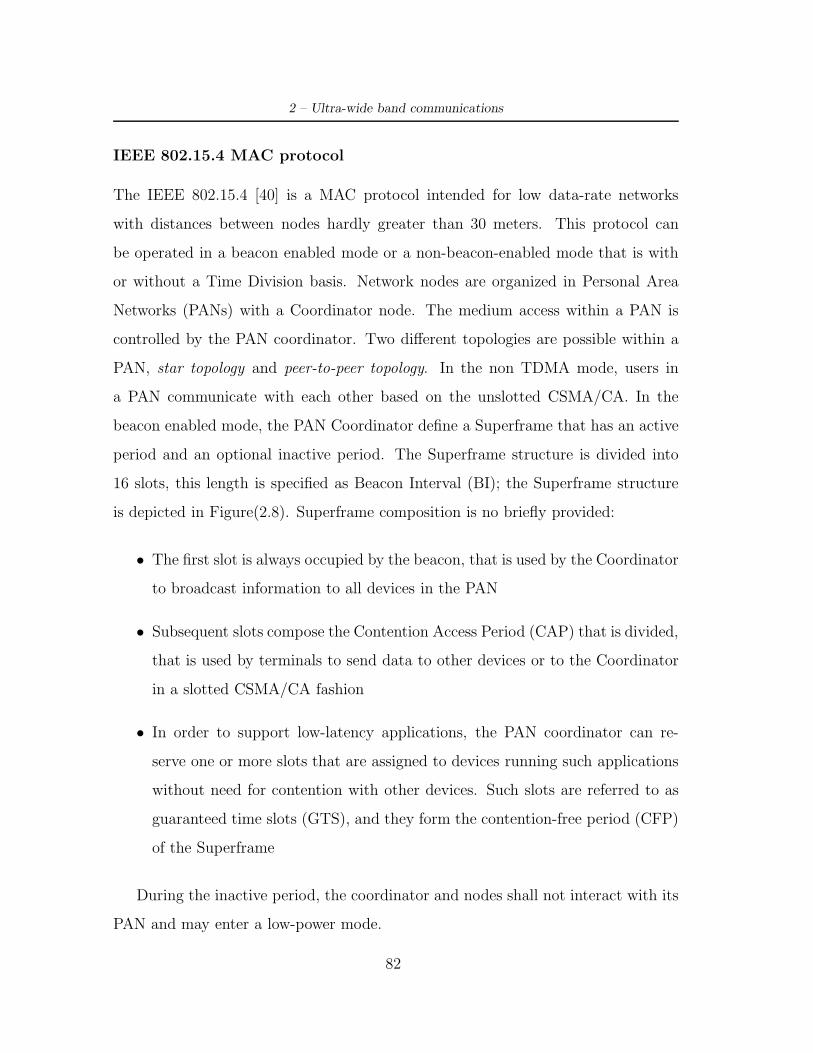
2 – Ultra-wide band communications
IEEE 802.15.4 MAC protocol
The IEEE 802.15.4 [40] is a MAC protocol intended for low data-rate networks
with distances between nodes hardly greater than 30 meters. This protocol can
be operated in a beacon enabled mode or a non-beacon-enabled mode that is with
or without a Time Division basis. Network nodes are organized in Personal Area
Networks (PANs) with a Coordinator node. The medium access within a PAN is
controlled by the PAN coordinator. Two di!erent topologies are possible within a
PAN, star topology and peer-to-peer topology. In the non TDMA mode, users in
a PAN communicate with each other based on the unslotted CSMA/CA. In the
beacon enabled mode, the PAN Coordinator define a Superframe that has an active
period and an optional inactive period. The Superframe structure is divided into
16 slots, this length is specified as Beacon Interval (BI); the Superframe structure
is depicted in Figure(2.8). Superframe composition is no briefly provided:
• The first slot is always occupied by the beacon, that is used by the Coordinator
to broadcast information to all devices in the PAN
• Subsequent slots compose the Contention Access Period (CAP) that is divided,
that is used by terminals to send data to other devices or to the Coordinator
in a slotted CSMA/CA fashion
• In order to support low-latency applications, the PAN coordinator can re-
serve one or more slots that are assigned to devices running such applications
without need for contention with other devices. Such slots are referred to as
guaranteed time slots (GTS), and they form the contention-free period (CFP)
of the Superframe
During the inactive period, the coordinator and nodes shall not interact with its
PAN and may enter a low-power mode.
82

2.5 – MAC Protocols for Low Data Rate UWB
Figure 2.8. An example of Superframe structure for 802.15.4 MAC.
If TDMA is not adopted, beacons are no longer needed for the definition of a
slotted time axis, but they are still required for broadcasting the ID of the PAN and
allow association of new devices. Unslotted CSMA/CA makes peer-to-peer data
exchange di"cult, since no common synchronization is available between devices,
and in the Standard it is not provided any specific synchronization procedure.
UWB2 MAC protocol
The Uncoordinated, Wireless, Baseborn Medium Access for UWB Communication
Networks referred as UWB2 [2], is a MAC protocol specifically designed for Impulse
Radio Ultra Wideband systems. The multiple access scheme is based on the com-
bination of a common control channel provided by a common Time-Hopping (TH)
code with dedicated data channels associated to transmitter specific TH codes. The
proposed protocol also takes into account synchronization requirements, in fact each
transmitted packet has a synchronization trailer part, composed by a certain num-
ber M of pulses (M is known a priori by receivers and depends on the environment
conditions). To obtain synchronization with the transmitter the receiver use a ded-
icated correlator that is continuously searching for the synchronization trailer. This
83
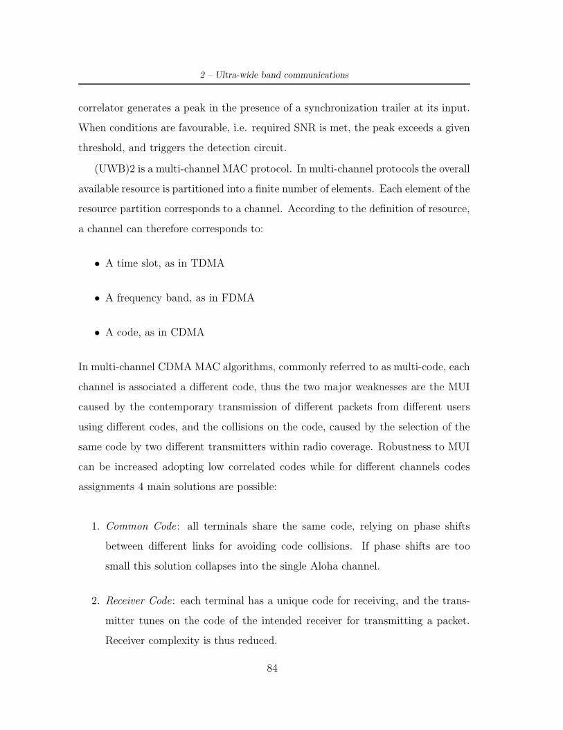
2 – Ultra-wide band communications
correlator generates a peak in the presence of a synchronization trailer at its input.
When conditions are favourable, i.e. required SNR is met, the peak exceeds a given
threshold, and triggers the detection circuit.
(UWB)2 is a multi-channel MAC protocol. In multi-channel protocols the overall
available resource is partitioned into a finite number of elements. Each element of the
resource partition corresponds to a channel. According to the definition of resource,
a channel can therefore corresponds to:
• A time slot, as in TDMA
• A frequency band, as in FDMA
• A code, as in CDMA
In multi-channel CDMA MAC algorithms, commonly referred to as multi-code, each
channel is associated a di!erent code, thus the two major weaknesses are the MUI
caused by the contemporary transmission of di!erent packets from di!erent users
using di!erent codes, and the collisions on the code, caused by the selection of the
same code by two di!erent transmitters within radio coverage. Robustness to MUI
can be increased adopting low correlated codes while for di!erent channels codes
assignments 4 main solutions are possible:
1. Common Code: all terminals share the same code, relying on phase shifts
between di!erent links for avoiding code collisions. If phase shifts are too
small this solution collapses into the single Aloha channel.
2. Receiver Code: each terminal has a unique code for receiving, and the trans-
mitter tunes on the code of the intended receiver for transmitting a packet.
Receiver complexity is thus reduced.
84

2.5 – MAC Protocols for Low Data Rate UWB
3. Transmitter code: each terminal has an unique code for transmitting, and the
receiver tunes on the code of the transmitter for receiving a packet. Receivers
must be able to listen to all possible codes in the network.
4. Hybrid : a combination of the above schemes.
Among these solutions, UWB2 adopts an Hybrid scheme for the specific case
of a TH-IR UWB system based on the combination of a common control channel,
provided by a Common TH code, with dedicated data channels associated to Trans-
mitter TH codes. The adoption of the Hybrid scheme is motivated by the authors as
it simplifies the receiver structure (data transmissions and corresponding codes are
transmitted on the common channel) and it provides a common channel for broad-
casting that is a key property for the operation of higher layers protocols. Broadcast
messages are for example required for routing and distributed positioning protocols.
The packet exchange procedure described below show that UWB2 also exploits the
ranging capability o!ered by UWB. Distance information between transmitter and
receiver is in fact collected during control packets exchange. Such information can
enable optimizations of several MAC features, and allow the introduction of new
functions, such as distributed positioning.
In the following procedure is assumed that, at each terminal T, MAC Protocol
Data Units (MACPDUs) resulting from the segmentation/concatenation of MAC
Service Data Units (MACSDUs) are stored in a transmit queue. It is also assumed
that T is able to determine how many MACPDUs in the queue are directed to a
given receiver R.
The transmission procedure Terminal T periodically checks the status of the
its MACPDUs queue and if there are data to transmit the terminal enable the
transmission procedure which can be described as follows:
1. The ID of the intended receiver R is extracted from the first PDU in the queue;
85
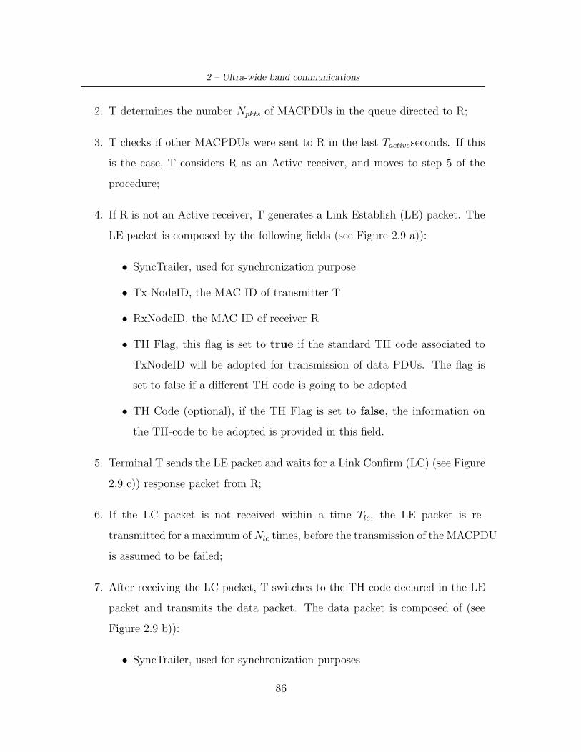
2 – Ultra-wide band communications
2. T determines the number Npkts of MACPDUs in the queue directed to R;
3. T checks if other MACPDUs were sent to R in the last Tactiveseconds. If this
is the case, T considers R as an Active receiver, and moves to step 5 of the
procedure;
4. If R is not an Active receiver, T generates a Link Establish (LE) packet. The
LE packet is composed by the following fields (see Figure 2.9 a)):
• SyncTrailer, used for synchronization purpose
• Tx NodeID, the MAC ID of transmitter T
• RxNodeID, the MAC ID of receiver R
• TH Flag, this flag is set to true if the standard TH code associated to
TxNodeID will be adopted for transmission of data PDUs. The flag is
set to false if a di!erent TH code is going to be adopted
• TH Code (optional), if the TH Flag is set to false, the information on
the TH-code to be adopted is provided in this field.
5. Terminal T sends the LE packet and waits for a Link Confirm (LC) (see Figure
2.9 c)) response packet from R;
6. If the LC packet is not received within a time Tlc, the LE packet is re-
transmitted for a maximum of Nlc times, before the transmission of the MACPDU
is assumed to be failed;
7. After receiving the LC packet, T switches to the TH code declared in the LE
packet and transmits the data packet. The data packet is composed of (see
Figure 2.9 b)):
• SyncTrailer, used for synchronization purposes
86

2.5 – MAC Protocols for Low Data Rate UWB
• Header, including the fields TxNodeID, RxNodeID, PDUnum and Npkts
• Payload, containing data information
8. Once the transmission is completed, T checks again the status of the data
queue, and repeats the procedure until all MACPDUs in the transmit queue
are served.
Synch Trailer Rx Node ID
Tx Node ID TH-code
TH-ag
x bits 16 bits 16 bits 1 bits 16 bits
a)
Synch Trailer Rx Node ID
Tx Node ID
PDUnum
x bits 16 bits 16 bits 8bits
b) Npkts
8bits
PAYLOAD
L bits
Synch Trailer Rx Node ID
Tx Node ID
x bits 16 bits 16 bits
c)
Figure 2.9. UWB2 MAC protocol packet structures, a) Link Establish (LE)packet, b) Data packet and, c) Link Confirm (LC) packet.
Reception procedure This is the procedure a terminal R in Idle state executes
when while listening to the Common TH code, a SyncTrailer is detected.
1. R checks the Rx Node ID field. If the value in the field is neither the MAC ID
of R nor the broadcast ID, the reception is aborted and the reception procedure
ends;
2. Since in the following we are not considering broadcast packets, let us assume
that the Rx Node ID contains the MAC ID of R. In this case, since R is
87

2 – Ultra-wide band communications
assumed in Idle state, MACPDUs directed to this terminal will necessarily be
LE packets;
3. Following the reception of a LE packet, R creates a LC packet, composed of
(see Figure 2.9 c)):
• SyncTrailer, used for synchronization purposes
• TxNodeID, the MAC ID of T
• RxNodeID, the MAC ID of R
4. R sends the LC packet and moves in the Active state, listening on the TH
code indicated in the LE packet. If no data packet is received within a time
Tdata the receiver falls back to Idle state and the procedure ends;
5. When a data packet is received, R processes the payload, and extracts Npkts
from the header. If Npkts > 0, R remains in Active state, since at least Npkts
more data packets are expected to be received from T. If Npkts = 0, R goes
back to the Idle state.
It should be noted that the above procedures are related to the setup of a single
link. During the reception procedure for example R also keeps on listening to the
common code. A terminal in fact can act as a receiver on one or more links while
acting as a transmitter on other links.
88

Chapter 3
convergence IR-UWB
3.1 convergence IR-UWB
Given the strong similarities between impulse radio UWB and wireless optical, the
combination of the two technologies can provide strong benefits and overcome limi-
tations characterizing both systems. In this section we will propose the combination
of the two physical layers by adopting a common medium access control protocol.
The choice of the most suitable physical layer can follow several strategies, specifi-
cally we consider two di!erent casses: minimization of the overall bit error rate and
minimization of the power consumption of the nodes (i.e. the higher the interference
level, the higher the number of necessary retransmissions to obtain the same BER
target).
While optical communication systems can operate everywhere without any spe-
cific regulatory permission, UWB radio, is subject to strong power limitations due
to its wide band that can potentially overlap with pre-existing wireless services. As
a consequence UWB links are sensible to the e!ect of strong narrowband interferers
that can jam the UWB signal and adversely a!ect performance (see section 2.4).
89
3 – convergence IR-UWB
This issue is particularly relevant in specific application scenarios where such nar-
rowband interferers are inherently present: this is the case for example of medical
premises, where diagnostic machines can emit RF radiations while operating, and of
industrial environments. In such scenarios network performance can be significantly
improved thanks to the adoption of an alternative physical layer solution based on
Di!use Wireless Optical (DWO) technology.
Furthermore, the similarities between UWB and DWO signal formats and charac-
teristics suggest that medium access control protocol schemes proposed for IR-UWB
can be used for both technologies, thus leading to a straightforward convergence of
UWB and DWO. In this work we evaluate the feasibility of this approach, by propos-
ing a solution for combining the two technologies by means of an environment-aware
physical layer selection strategy. The performance of the two physical layers solu-
tions is evaluated by simulations in order to determine the potential performance
increase guaranteed by the adoption of the proposed strategy.
3.2 Switching physical layer
The physical layer of the proposed dual system is able, if necessary, to switch from
a technology to another according to a predefined rule. The optical part of the
considered system is a Di!use Wireless Optical physical layer with an OOK mod-
ulation. Since we are interested in low cost transmission systems, the considered
transmitter is an infrared LED with wavelength of possibility of 850 nm (instead
of, for example, a more expensive laser diode). We evaluate the performance of the
DWO system both in the case of absence of a channel coding and in the case of
Optical Orthogonal Codes. Provided simulations will show the improvements due
to the presence of the code. On the other hand, the UWB physical layer part, is a
2 level PPM system, that uses Time Hopping codes.
90

3.2 – Switching physical layer
As previously mentioned, we propose two di!erent physical layer switching strate-
gies. The first is aimed at straightforwardly minimizing the whole system BER,
therefore, the selection is based on the rule:
PHY = argmin{BERUWB,BERDWO} (3.1)
where BERUWB is the bit error rate measured on the UWB physical layer and
BERDWO is the bit error rate measured on the di!use optical wireless physical
layer. Both BER values can be measured either on the basis of previous data pack-
ets exchange, or by means of beacon packets sent on the two physical layer interfaces.
The exact definition of the procedure for obtaining such measurements is outside
the scope of this work, and is left for future investigation.
The goal of the second switching strategy is minimizing the consumed energy
of each node due to the transmissions and receptions of packets. In this case the
selection of the physical layer is carried out according to the following rule:
PHY = argmin{CUWB · BERUWB,CDWO · BERDWO} (3.2)
where CUWB and CDWO are the cost of the transmission of one bit, for the UWB PHY
and the DWO PHY, respectively. This case can be considered as a general case pro-
vided that the former strategy can be obtained setting CUWB = CDWO = 1. The ba-
sic principle of this latter strategy, is that if transmitting a bit using the UWB physi-
cal layer has a higher energy cost than transmitting the same bit with DWO physical
layer, DWO should be preferred to some extent also when BERDWO > BERUWB.
The value of the two coe"cients would thus depend on hardware, physical layer
settings (e.g. code selection) and MAC settings (retransmission strategy and MAC
layer FEC coding). In the following part of this work system simulation results are
provided for the first switching strategy, that is we consider both the cost coe"cient
91

3 – convergence IR-UWB
to be equal to one. The resulting system is thus aimed at minimizing overall BER
i.e. the chosen physical layer is the one that provides a lower bit error rate.
3.2.1 Energy consumption for UWB systems
Aimed at evaluating the energy consumption due to the transmission and/or recep-
tion of one packet, we study the case of an UWB system. Our goal is to evaluate
how much energy is consumed by a single node of the network when it is involved
in transmitting or receiving one packet. We based our model on the framework for
energy-evaluation defined in [41]; here the authors show how power consumption
depends on hardware characteristics of the transceiver, physical layer settings (e.g.
code selection) and MAC settings like retransmission strategy and MAC layer cod-
ing. We now describe the energy consumption rule for the transmission of a packet
followed by the consumption for a reception. For our UWB system, the energy
consumed by a node when a packet of size Packetsize is sent at low bitrate, can be
expressed by the sum of two main components, the startup energy Estartup and the
e!ective transmission energy:
EnergyTX = Estartup + Packetsize ·'ETXperbit
+ ETXprop · dα(
(3.3)
where ETXperbitis the energy that is necessary to transmit a single bit, ETXprop is the
dissipated energy of the transmitting amplifier, d is the distance between transmitter
and receiver and ! is the exponent of the power attenuation low of the environment.
The energy necessary for the reception of a packet of size Packetsize for the same
system is expressed by:
EnergyRX = Estartup + Packetsize · ERXperbit(3.4)
In the original model (see [41]) also a term that depends on the decoding algorithm
is used, however since we do not consider channel coding, we decided to neglect that
92

3.2 – Switching physical layer
term. We adopted the presented consumption model with a low data rate UWB
system in the presence of narrow band interferers, as it is shown in Figure (4.5),
as the interfering power increases the energy consumption grows up because of the
higher number of retransmissions (and receptions) necessaries.
3.2.2 Optical Quantum Limit
The considered optical receiver is a direct detection system, so the detector converts
the received power into an electrical current. The received signal at the optical
detector output is always non-negative (because power is always non-negative) and
random due to the random arrival times of photons. This is not a flaw in the detec-
tor, but rather is a fundamental law of physics as dictated by quantum mechanics.
Quantum e!ects are present but insignificant at microwave frequencies and below,
but are important at optical frequencies typically in the near-infrared band. If we
consider an ideal receiver in which all impairments are absent, and we want to de-
termine the error probability, there is a fundamental limit we cannot neglect, the
Quantum Limit [42].
Consider a single transmitter-receiver couple. If we were magically able to elim-
inate all other sources of noise, and were able to reliably detect a photo-electron
in the receiver circuitry, then we could use the following receive criterion: no pulse
was transmitted if we receive zero photo-electrons, and a pulse was transmitted if
we receive one or more photo-electrons in the symbol interval. If we assume that no
dark current is present and a perfect quantum e"ciency (( = 1, that is all the light
energy is converted in electrical energy), the arrival rate of photo-electrons is:
#(t) =P (t)
h · $ (3.5)
where P (t) is the received optical power and h · $ is the energy of one photon (h is
93

3 – convergence IR-UWB
the Planck’s constant and $ is the frequency of one photon). The number of photo-
electrons observed during a symbol interval is a Poisson distributed random variable
with parameter (, where ( is the integral of #(t) over the symbol period. Thus,
when a pulse is transmitted (( > 0) the probability of n received photo-electrons is:
p(n) =(ne−!
n!(3.6)
Since the integral of power is energy,
( =Eb
h · $(3.7)
where Eb is the total received energy in the symbol interval. Since h ·$ is the energy
of one photon, another interpretation of ( is the average number of photons arriving
at the detector in one symbol interval.
Quantum e!ects are negligible at microwave frequencies because since this fre-
quencies are about five orders of magnitude smaller than optical frequencies, the
energy per photon is five orders of magnitude smaller, and for a given received pulse
energy the average number of photons is five order of magnitude larger. Since that
the variance of the Poisson distribution in (3.6) is equal to the mean, the standard
deviation is the square-root of the mean. The width of the distribution, as defined
by the standard deviation divided by the mean, approaches zero as the mean gets
large. Thus, for a very large number of received photons, the width of the Poisson
distribution approaches to zero, and the randomness due to quantum e!ects be-
comes negligible.
According to [42] for idealized receiver with no interferences no error can be
made if no pulse is transmitted, since precisely no photons will be received. Hence
the only error that is possible result if a pulse is transmitted and no photons are
94
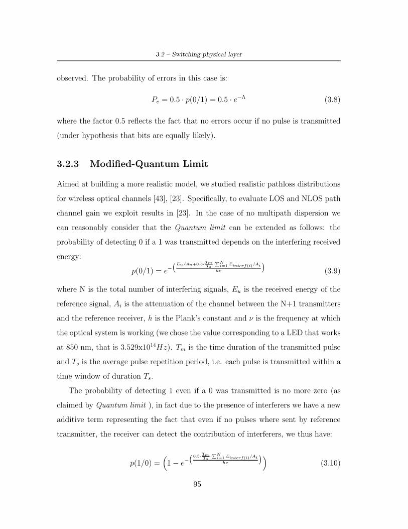
3.2 – Switching physical layer
observed. The probability of errors in this case is:
Pe = 0.5 · p(0/1) = 0.5 · e−! (3.8)
where the factor 0.5 reflects the fact that no errors occur if no pulse is transmitted
(under hypothesis that bits are equally likely).
3.2.3 Modified-Quantum Limit
Aimed at building a more realistic model, we studied realistic pathloss distributions
for wireless optical channels [43], [23]. Specifically, to evaluate LOS and NLOS path
channel gain we exploit results in [23]. In the case of no multipath dispersion we
can reasonably consider that the Quantum limit can be extended as follows: the
probability of detecting 0 if a 1 was transmitted depends on the interfering received
energy:
p(0/1) = e−)Eu/Au+0.5·Tm
Ts·PN
i=1 Einterf(i)/Aih$
*(3.9)
where N is the total number of interfering signals, Eu is the received energy of the
reference signal, Ai is the attenuation of the channel between the N+1 transmitters
and the reference receiver, h is the Plank’s constant and $ is the frequency at which
the optical system is working (we chose the value corresponding to a LED that works
at 850 nm, that is 3.529x10¹⁴Hz). Tm is the time duration of the transmitted pulse
and Ts is the average pulse repetition period, i.e. each pulse is transmitted within a
time window of duration Ts.
The probability of detecting 1 even if a 0 was transmitted is no more zero (as
claimed by Quantum limit ), in fact due to the presence of interferers we have a new
additive term representing the fact that even if no pulses where sent by reference
transmitter, the receiver can detect the contribution of interferers, we thus have:
p(1/0) ='1 ! e−
) 0.5·TmTs
·PN
i=1 Einterf(i)/Aih$
*((3.10)
95
3 – convergence IR-UWB
So the overall bit error probability can be expressed by sum of two equally like
contributions:
Pe = 0.5 · p(0/1) + 0.5 · p(1/0) (3.11)
According to the proposed performance evaluation method based on the quantum
limit approach, varying the time duration of the optical transmitted pulse Tm, that
is choosing di!erent types of LEDs, will influence the bit error rate. In Figure (3.1)
a simulation result of this e!ect is shown. In the Figure we consider two di!erent
scenarios, the first with all nodes of the network in visibility (NLOSprob = 0) and
the second in which some of the nodes can not communicate with the direct link,
that is for all the nodes there is a given probability (NLOSprob = 0.3) that they
are not in visibility. The simulated networks are composed by 10 nodes randomly
positioned within a square room of 12mx12m, the average transmitter power is fixed
at 1mW and the transmission rate of each node is 10kbps. As can be seen, if Ts is
constant, increasing the pulse duration increases the BER in both cases.
10−9 10−8 10−70.02
0.03
0.04
0.05
0.06
0.07
0.08
0.09
0.1
Pulse duration Tm [s]
BER
NLOSprob=0.3NLOSprob=0
Figure 3.1. BER variation due to a di!erent time duration of the transmitted opti-cal pulse with the same average transmitted power of 1mW and 10 nodes randomlypositioned within a square room of 12mx12m.
96

3.2 – Switching physical layer
3.2.4 Di!use wireless optical channel performance using OOC
For the performance evaluation of a DWO system that adopts optical orthogonal
codes we refer to [9] were Inter Symbol Interference (ISI) and MUI are considered.
The adopted indoor channel impulse response follows the ceiling bounce model de-
scribed in section (1.2.2) that is expressed by equation (1.13). According to [15]
with an OOC code (n,w,1,1) the maximum number of user that can transmit at the
same time is limited by:
N ";
n ! 1
w(w ! 1)
<
(3.12)
where n is the number of chips of the code and w is the weight of the code, that is
the number of ”1” within the n chips. If a synchronous system is considered and
the hypothesis that the received interfering power is equal to the desired power, we
define the amount of interference due to ISI that the chip kth causes on the chip jth
as pi(k,j). Because of ISI also the desired signal introduces some interference, that
is the interference produced by the desired chip kth on the desired chip jth, this is
expressed by: pd(k,j). Expressions for pi(k,j) and pd(k,j) are given by:
pi(k,j) = pd(k,j) = hj−k (k " j) (3.13)
where hk is the equivalent discrete-time impulse response of the system sampled at
rate 1/Tc where Tc is the chip duration. An expression of hk is:
hk = pTc & h(t) & g(t) (3.14)
where pTc is a rectangular pulse with duration 0 " t " Tc an g(t) is the transmitted
pulse waveform. The number of user that are causing interference is referred as
pMUI . If the interfering signal stands exactly on the same chip of the desired signal
pMUI = h0 otherwise pMUI = 0. The e!ect of multipath distortion is spreading the
signal over di!erent chips causing thus ISI on the received signal. The amount of
interference that a single user can perceive on his desired signal can be evaluated
97

3 – convergence IR-UWB
considering the all the possible combination of the codes. When the desired user
transmits 0 or 1, we denote the amounts of interference to the desired signal by P0
and P1 respectively. Expressions of P0 and P1 are:
P0 =n−1"
j=0
n−1"
k=0,k )=j
pi(k,j) + pMUI (3.15)
P1 =n−1"
j=0
n−1"
k=0,k )=j
{pi(k,j) + pd(k,j)} + pMUI (3.16)
At the receiver the signal is correlated and only the interferences on the same chips
of the desired signal are added. These added interferences can be denoted by Pm0
and Pm1 respectively. The mean BER can be evaluated averaging all the possible
combination of w “1” within n chips called ' and be expressed by:
BER =1
F (N−1)23(N−1)
""
i=1
=0.5 · Q{'(2b ! Pm0,i
w) + 0.5 · Q{'(2A ! 2Pm1,i
w! 2b)}
>
(3.17)
where
' =G0PTX)
2
#nTc
w+2(3.18)
where b is the receiver threshold of the receiver, N is the possible number of users
depending on the code, A is the received signal in the desired chip place, +2 is
the power spectral density of the thermal noise present at the output of the pho-
todetector, PTX is the average transmitted power, and ) is the responsivity of the
receiver.
3.3 MAC for Low Data Rate Impulsive systems
Wireless access is not only the action of accessing, that is connecting to, a fixed
network but also but more in general, the action of accessing the wireless medium.
This is in fact, the available resource that has to be shared among the nodes of the
98
3.3 – MAC for Low Data Rate Impulsive systems
network is the wireless medium.
The wireless access can be centralized or distributed, in the case of centralized
the resource available to the system is managed and controlled by a central unit
that is the network coordinator. All the units that want to join, leave or transmit
in the network must refer to this unit. In decentralized access systems, all nodes
are hierarchically equivalent (there is not a central unit with MAC access functions)
and they can cooperate for the purpose of resource sharing. A typical example of
centralized access network is the IEEE 802.11 system in which the role of the central
unit is covered by an Access Point unit (or Hot Spot) which is an element connected
to the fixed network and that coordinates the access of wireless devices by managing
the resource available in the system for transmissions. Other examples are cellular
networks like GSM or UMTS networks. A typical example of decentralized access
networks is an ad-hoc network. In ad-hoc networks nodes can be cooperative or
non-cooperative in finding routes to reach other nodes, in controlling the transmit-
ting power aimed at not interfering among them or in organizing the structure of
the network.
The MAC protocol we used in our simulations is the UWB2 protocol that has
been already described in the section (2.5). This protocol is specifically designed for
IR UWB signal, however, thanks to the impulsive nature of optical signals it can
reasonably be exploited in the studied context.
99

3 – convergence IR-UWB
100
Chapter 4
Simulation results and Conclusions
4.1 The pulse collision model validation
The pulse collision model defined in [2],[36] and described in section (2.3.1) pro-
vides a possible approach for BER evaluation for an IR-TH-UWB system in the
presence of other IR-TH-UWB interfering users. Since the UWB physical layer of
our dual physical layer system is a pulse based TH-UWB system, we are particu-
larly interested in adopting the UWB2 MAC protocol (see section 2.5) that is based
on the pulse collision model. As reported in the relative section we are interested
in validating simulation results produced by the authors of the model, and more
specifically we want to analyze the model behaviour while increasing the number
of pulses per bit Ns while maintaining constant the transmitted average power per
node PTX and the user data rate Rb, i.e. we vary average pulse repetition period Ts
(since Rb = 1/(Ns · Ts)). Computer simulations show that increasing Ns provides
an higher BER, this is because even if the transmitted average power of di!erent
nodes is constant, the useful received energy Eu is reduced due to a shorter average
pulse repetition period. In Figure (4.1) three di!erently populated networks are
simulated: as the number of pulses per bit is increased, the system performance in
101

4 – Simulation results and Conclusions
term of Bit Error Rate slightly worsens.
3 4 5 6 7 8 9
10−5
10−4
10−3
Ns
BER
BER vs. Ns
10 nodes20 nodes30 nodes
Figure 4.1. BER vs. Ns for di!erent populated networks, according to the pulsecollision model increasing Ns does not improve the performance.
With respect to the pulse collision model defined in the literature, we must state
that in our simulations we made the hypothesis that even if two packets overlap
each other only for an " > 0 amount of time we consider that they collide for the
entire packet duration. This is, of course, a worsening hypothesis that was dictated
by implementation complexity of the model. The worsening e!ect of this hypothesis
can be highlighted if we simulate an UWB system increasing the number of pulses
per bit Ns while maintaining constant the average pulse repetition period Ts. As
it is depicted in Figure (4.2), if we increase Ns but fix Ts, we are reducing the bit
rate Rb = 1/(TsNs), thus a packet with the same length will need more time to be
transmitted incrementing the probability of having a packet collision. In the Figure,
we show how the number of all interfering packets Ni (sum of the interfering packets
perceived by all users) normalized by the number of users in the network and the
number of received packets (sum of all packets, desired and interfering, received by
all users) increases as Ns increases.
On the other hand if we want the bitrate to remain constant at approximately
102

4.1 – The pulse collision model validation
3 4 5 6 7 8 9 10 110.1
0.2
0.3
0.4
0.5
0.6
0.7
0.8
Ns
(Sum
(Ni))
/(Num
node
s*Sum
(rece
ived
pack
ets)
) Average number of Ni vs Ns
10 nodes20 nodes30 nodes
Figure 4.2. Average number of interfering packets Ni as a function of the numberof pulses per bit Ns. Maintaining fixed Ts while increasing Ns cause more collisions.
1Mbps, while increasing the number of pulses per bit, the average pulse duration Ts
must be reduced accordingly. Figure (4.3) shows how in this case, an higher number
of pulses per bit gives the rise to a lower number of interfering packets in the air.
3 4 5 6 7 8 90.04
0.06
0.08
0.1
0.12
0.14
0.16
0.18
Ns
(Ave
rage
Ni)/
(Num
node
s*Rec
eive
d pa
cket
s)
10 nodes20 nodes
Figure 4.3. Average number of interfering packets Ni as a function of the numberof pulses per bit Ns; in this case Ts is reduced with increasing Ns, thus the bitrateRb remains approximately of 1Mbps.
103
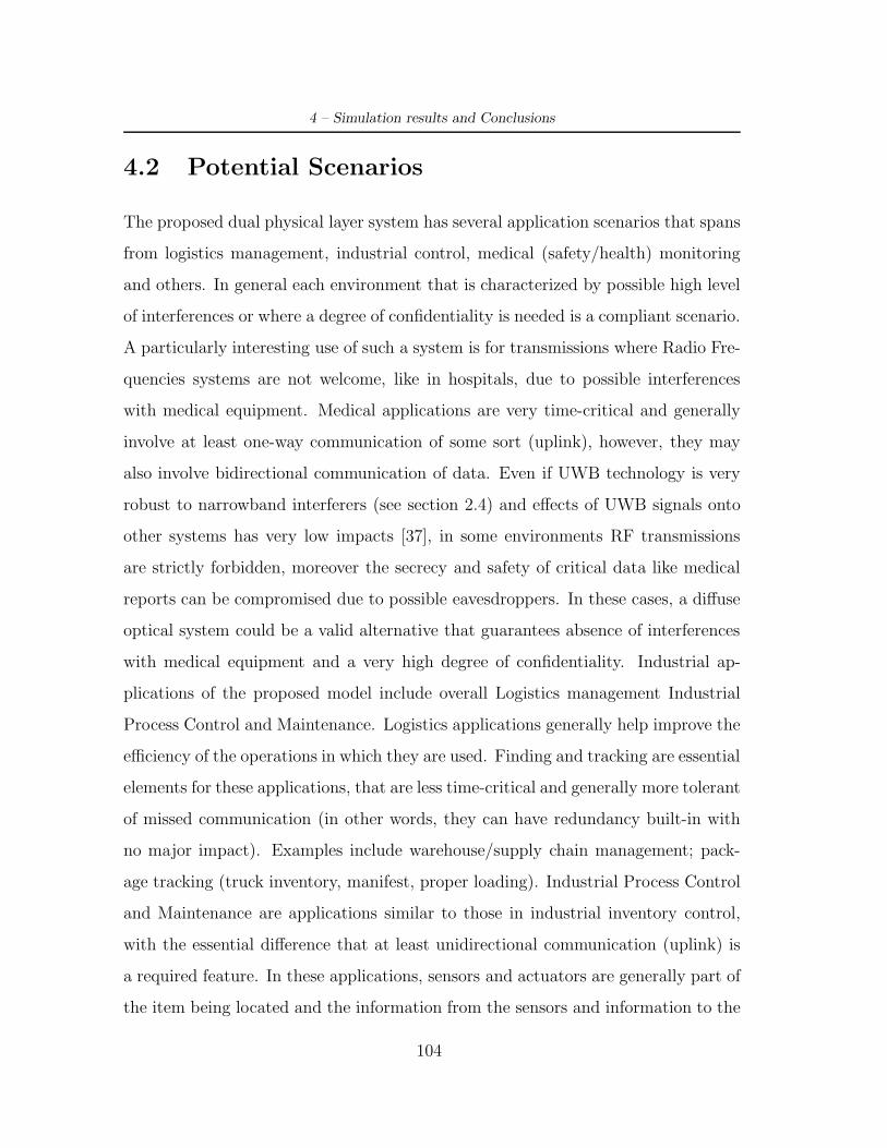
4 – Simulation results and Conclusions
4.2 Potential Scenarios
The proposed dual physical layer system has several application scenarios that spans
from logistics management, industrial control, medical (safety/health) monitoring
and others. In general each environment that is characterized by possible high level
of interferences or where a degree of confidentiality is needed is a compliant scenario.
A particularly interesting use of such a system is for transmissions where Radio Fre-
quencies systems are not welcome, like in hospitals, due to possible interferences
with medical equipment. Medical applications are very time-critical and generally
involve at least one-way communication of some sort (uplink), however, they may
also involve bidirectional communication of data. Even if UWB technology is very
robust to narrowband interferers (see section 2.4) and e!ects of UWB signals onto
other systems has very low impacts [37], in some environments RF transmissions
are strictly forbidden, moreover the secrecy and safety of critical data like medical
reports can be compromised due to possible eavesdroppers. In these cases, a di!use
optical system could be a valid alternative that guarantees absence of interferences
with medical equipment and a very high degree of confidentiality. Industrial ap-
plications of the proposed model include overall Logistics management Industrial
Process Control and Maintenance. Logistics applications generally help improve the
e"ciency of the operations in which they are used. Finding and tracking are essential
elements for these applications, that are less time-critical and generally more tolerant
of missed communication (in other words, they can have redundancy built-in with
no major impact). Examples include warehouse/supply chain management; pack-
age tracking (truck inventory, manifest, proper loading). Industrial Process Control
and Maintenance are applications similar to those in industrial inventory control,
with the essential di!erence that at least unidirectional communication (uplink) is
a required feature. In these applications, sensors and actuators are generally part of
the item being located and the information from the sensors and information to the
104
4.3 – Simulated scenario
actuators needs to be communicated. Examples include wireless sensor networks;
large structures monitoring; aircraft/ground vehicle anticollision; and monitoring,
sensing and control of industrial and environmental processes.
4.3 Simulated scenario
The simulated environment is an indoor square room of 12mx12m with the ceiling
height of 3m. The nodes of the network are always randomly located within the room
area and they can be in visibility or not with a certain probability (NLOSprobability)
that is a simulation parameter. The instantaneous transmission rate of each node
is supposed to be fixed at Rb = 966Kbps, i.e. since Rb = 1/Tb = 1/(NsTs), if more
than a pulse per bit are transmitted the average pulse repetition time is reduced
accordingly. Packets of each node are generated according to a Poisson generation
process. The transmitted packet is composed by a payload of 1224 bits and an
header of 64 bits that is used by the MAC layer for synchronization issues like de-
scribed in section (2.5). Since the initial position of the nodes is randomly generated
and there is no mobility in the system, all simulations are averaged over 10 runs and
each run simulates the network behaviour for 3000 seconds.
The MUI model used in the simulations is the Pulse Collision model (see section
2.3.1) for both UWB and DWO systems. In order to model the impact of channel
we adopted the first two channel scenarios defined within the 802.15.4a TG, that
is CM1 and CM2, corresponding to indoor Line Of Sight (LOS) and Non-Line Of
Sight (NLOS) channel conditions, respectively [44].
The UWB physical layer settings can be summarized as follows:
• IR-UWB with a band of 494 MHz centered at 3952 MHz (corresponding to
105

4 – Simulation results and Conclusions
Channel 2 of the 802.15.4a channel scheme);
• Average Pulse Repetition Frequency (PRF): 2.895 MHz;
• Pulses Per Symbol (Ns): 3,5 or more;
• Modulation: 2-PPM;
• TX power PTX : fixed to FCC indoor limit [28], leading for the considered
bandwidth to PTX = 36.6 µW .
• TH-coding with pseudorandom codes.
The presence of narrowband interference (NBI) was also introduced in the UWB
physical layer model. The NBI was modeled as an additive white Gaussian noise
that sums up with the thermal noise, see section (2.4) for more details. The value of
the spectral density of such additional noise depends on the power spectral density
and the actual bandwidth of the NBI.
The DWO physical layer settings can be summarized as follows:
• Modulation: OOK;
• Transmitter type: infrared LED # = 850nm;
• Pulses Per Symbol (Ns): 1 or more if OOC codes are used;
• TX power PTX : various values from 10−4W to 1W.
4.4 Simulation results
All computer simulations performed in this work were made using the open source
discrete event simulation system OMNeT++.
106

4.4 – Simulation results
4.4.1 UWB system
Narrow Band Interferences In the presence of narrow band interferers like
Fixed Wireless systems, a cellular system or a medical equipment, UWB perfor-
mance are severely reduced. Even though narrowband signals interfere with only
a small fraction of the UWB spectrum, due to their relatively high power with re-
spect to the UWB signal, the performance and capacity of UWB systems can be
considerably a!ected. Figure (4.4) presents the throughput, that is the ratio of the
correctly received packets to the total number of received packets, for two di!erent
UWB systems one adopting Ns = 3 and the other with Ns = 5 as a function of the
narrow band interferer PSD that is modeled as an additional Gaussian noise.
10−20 10−19 10−18 10−17 10−160
0.1
0.2
0.3
0.4
0.5
0.6
0.7
0.8
0.9
1
Narrow Band Interference PSD [V2/Hz]
Thro
ughp
ut
Ns=3Ns=5
Figure 4.4. Throughput in the case of UWB physical layer with Ns = 3 andNs = 5 for a network of 10 nodes with NLOSprobability=0.3 as a function of thepower spectral density of a narrow band interferer NNBI .
For the same scenario of 10 UWB nodes in the presence of narrow band interfer-
ers, we can evaluate the energy consumption necessary for the transmission/reception
procedures of each node. The function for the evaluation of the energy consump-
tion for a UWB low bitrate system was described in section (3.2.1). As one can
reasonably suppose if a narrow band interferer is present each UWB node will be
107

4 – Simulation results and Conclusions
forced to transmit several times the same packets and consequently perform several
times both the transmission and reception procedure. In Figure (4.5) the energy
consumption of each node in the presence of narrowband interferers is presented.
The average “cost” of transmission is normalized by the number of correctly received
packets.
1e−20 1e−19 1e−18 1e−17 1e−160
0.5
1
1.5
2
2.5
3x 10⁻³
Narrow Band Interference PSD [V2/Hz]
Per p
acke
t ene
rgy
cons
umpt
ion
[J] Ns=3
Ns=5
Figure 4.5. Energy consumption for each node of the UWB network as afunction of the NBI PSD.
4.4.2 DWO system
According to the modified version of the quantum limit model previously presented,
in Figure (4.6) we show the system throughput for two di!erent scenarios, the first
with 5 nodes and the second with 10 nodes. In both cases the probability of NLOS
links is set to 0.3. Note that with this settings throughput increases when trans-
mitted power increases, however it is clear that if the optical power is higher than
1mW the system saturate in both cases, due to the more and more relevant MUI
weight in the error probability formula (3.10).
108

4.4 – Simulation results
10−4 10−3 10−2 10−1 1000.5
0.55
0.6
0.65
0.7
0.75
0.8
Transmitted power [W]
Thro
ughp
ut
5 nodes10 nodes
Figure 4.6. Throughput in the case of two di!erently populated networkswith NLOSprobability set to 0.3 as a function of the transmitted opticalpower of the LED.
4.4.3 CIRCUS system
Aimed at defining a system able to switch its physical layer technology from UWB to
Optical, we analyzed both systems separately to show how switching from a system
to another may conduct to better performance. We exploited previous simulation
results and we build up a Figure representing the dual system communicating in
an indoor environment. Actually the default technology of current system is the
UWB and the transmission is characterized by a TH code and a number of pulses
per bit equal to 5. Let this UWB system transmits in the presence of a narrowband
interferer with a power spectral density of 10−20 [V 2/Hz], current BER value would
be approximately 3·10−5. If at the time t0 another narrowband system characterized
by an higher power spectral density of 10−6 [V 2/Hz] would enter the same room,
performance of the UWB system would instantly worsen. The impact of the ulterior
interferer would be the growth of the BER up to a value of about 0.047. In the same
scenario an optical di!use system would not be influenced by RF interferers. Based
on the modified quantum limit approach, an optical network with 5 nodes that do
109
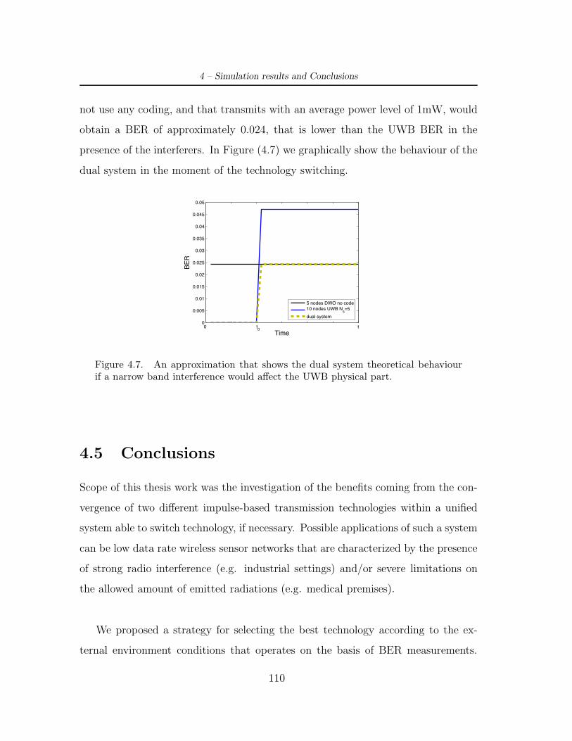
4 – Simulation results and Conclusions
not use any coding, and that transmits with an average power level of 1mW, would
obtain a BER of approximately 0.024, that is lower than the UWB BER in the
presence of the interferers. In Figure (4.7) we graphically show the behaviour of the
dual system in the moment of the technology switching.
0 t0
0.005
0.01
0.015
0.02
0.025
0.03
0.035
0.04
0.045
0.05
Time
BER
5 nodes DWO no code10 nodes UWB Ns=5dual system
t0
Figure 4.7. An approximation that shows the dual system theoretical behaviourif a narrow band interference would a!ect the UWB physical part.
4.5 Conclusions
Scope of this thesis work was the investigation of the benefits coming from the con-
vergence of two di!erent impulse-based transmission technologies within a unified
system able to switch technology, if necessary. Possible applications of such a system
can be low data rate wireless sensor networks that are characterized by the presence
of strong radio interference (e.g. industrial settings) and/or severe limitations on
the allowed amount of emitted radiations (e.g. medical premises).
We proposed a strategy for selecting the best technology according to the ex-
ternal environment conditions that operates on the basis of BER measurements.
110

4.5 – Conclusions
Thanks to the introduction of flexible coe"cients in the condition that leads to the
selection, di!erent performance goals can be pursued, ranging from simple BER
minimization to maximum energy e"ciency. Computer simulations analyzed the
e!ectiveness of the combination of the two technologies.
As previously mentioned, accordingly to the defined cost function for the physical
layer switching, we investigated a scenario where both the cost coe"cients are equal
to 1. A deep investigation on the energy consumption evaluation for an optical node,
can be a subject of further studies.
Future works can be also oriented on the definition of two “cost” coe"cients
(one for each physical layer) necessary for the implementation of the second proposed
physical layer switching method, the energy optimization. Would be also interesting
to study the introduction of Optical Orthogonal Codes and quantify the impact of
an increased robustness of the optical part of the system.
111

4 – Simulation results and Conclusions
112

Bibliography
[1] J. M. Kahn and J. R. Barry, “Wireless Infrared Communications,” Proceedings
of the IEEE, vol. 85, no. 2, February 1997.
[2] M.-G. DiBenedetto, L. D. Nardis, M. Junk, and G. Giancola, “(UWB)2:
Uncoordinated, Wireless, Baseborn, Medium Access Control for UWB com-
munication networks,” Mobile Networks and Applications, vol. 10, no. 5, pp.
663–674, 2005.
[3] M. D’amico, A. Leva, and B. Micheli, “Free-Space Optics Communication
Systems: First Results from a Pilot Field-Trial in the Surrounding Area of
Milan, Italy,” IEEE Microwave and Wireless Components Letters, vol. 13, no. 8,
pp. 305–307, August 2003.
[4] H. A. Willebrand and B. S. Ghuman, “Fiber optics without fiber,” Spectrum,
IEEE, vol. 38, no. 8, pp. 40–45, August 2001.
[5] Communication by Light CBL. [Online]. Available:
http://www.cbl.de/englisch/
[6] F. Gfeller and U. Bapst, “Wireless in-house data communication via di!use
infrared radiation,” Proceedings of the IEEE, vol. 67, no. 11, pp. 1474–1486,
november 1979.
[7] J. Carruthers, “Wireless infrared communications,” Wiley Encyclopedia of
Telecommunications, 2002.
113

Bibliography
[8] K. Langer and J. Grubor, “Recent developments in optical wireless communi-
cations using infrared and visible light,” ICTON, 2007.
[9] R. Matsuo, M. Matsuo, T. Ohtsuki, T. Udagawa, and I. Sasase, “Performance
analysis of indoor infrared wireless systems using ook cdma on di!use channels,”
1999.
[10] J. R. Barry, J. M. Kahn, W. J. Krause, E. A. Lee, and D. G. Messerschmitt,
“Simulation of multipath impulse response for indoor wireless optical channels,”
IEEE Journal on Selected Areas in Communications, vol. 11, no. 3, pp. 367–379,
April 1993.
[11] F. J. Lopez-Hernandez, E. Poves, R. Perez-Jimenez, and J. Rabadan, “Low-
Cost Di!use Wireless Optical Communication System based on White LED,”
ISCE ’06. 2006 IEEE Tenth International Symposium on Consumer Electron-
ics, no. 1-4, 2006.
[12] M. Audeh and J. Kahn, “Performance Evaluation of Baseband OOK for
Wireless Indoor Infrared LANs Operating at 100 Mb/s,” IEEE Transactions
on Communications, vol. 43, no. 6, pp. 2085–2094, June 1995.
[13] U. N. Griner and S. Arnon, “Multiuser Di!use Indoor Wireless Infrared
Communication Using Equalized Synchronous CDMA,” IEEE Transactions
on Communications, vol. 54, no. 9, pp. 1654–1662, September 2006.
[14] S. Han, “Optical CDMA with Optical Orthogonal Code,” Multiuser Wireless
Communication, 2002.
[15] F. R. K. Chung, J. A. Salehi, and V. K. Wei, “Optical Orthogonal Codes:
Design, Analysis, ans Applications,” IEEE Transactions on Information The-
ory, vol. 35, no. 3, p. 595604, May 1989.
[16] M. Choudhary, P. K. Chatterjee, and J. John, “Optical Orthogonal Codes
Using Error Correcting Codes,” 2002.
[17] The LEOT curriculum by the Center for Occupational Research and
114

Bibliography
Development (CORD). [Online]. Available: http://cord.org/cm/content1.htm
[18] J. MacChesney, “Fiber optics tutorial, Bell Labs, Lucent Technologies.”
[Online]. Available: http://www.arcelect.com/fibercable.htm
[19] B. E. A. Saleh and M. C. Teich, Fundamentals of Photonics. Wiley-
Interscience, 1991.
[20] D. Kedar and S. Arnon, “Urban optical wireless communication networks:
the main challenges and possible solutions,” IEEE Communications Magazine,
vol. 42, no. 5, pp. S2–S7, May 2004.
[21] X. Zhu and J. M. Kahn, “Free-Space Optical Communication through
Atmospheric Turbolence Channels,” IEEE Transactions on Communications,
vol. 50, no. 8, pp. 1293–1300, August 2002.
[22] S. Hranilovic, Wireless Optical Communication Systems, 1st ed. Springer,
September 2004.
[23] J. Carruthers, S. Carroll, and P. Kannan, “Propagation modelling for indoor
optical wireless communications using fast multi-receiver channel estimation,”
Optoelectronics, IEEE Proceedings, vol. 150, no. 5, pp. 473–481, October 2003.
[24] J. B. Carruthers and J. M. Kahn, “Modeling of Nondirected Wireless Infrared
Channels,” IEEE Transactions on Communications, vol. 45, no. 10, pp. 1260–
1268, October 1997.
[25] A. Sato, M. Asano, H. Uehara, and I. Sasase, “The Iinfluence of Multipath
Distortion on the Transmitted Pulse in Di!use Indoor Infrared Channels,”
Computer and Signal Processing Communications, vol. 2, no. 636-639, August
1997.
[26] A. J. C. Moreira, R. T. Valadas, and A. M. de Oliveira-Duarte, “Optical in-
terference produced by artificial light,” Wirel. Netw., vol. 3, no. de Oliveira
Duarte A.M., pp. 131–140, 1997.
115
Bibliography
[27] V. Vitsas and A. C. Boucouvalas, “Performance analysis of the advanced in-
frared (Air) CSMA/CA MAC protocol for wireless LANs,” Wirel. Netw.,
vol. 9, no. 5, pp. 495–507, 2003.
[28] FCC, “Revision of part 15 of the commission’s rules regarding ultra-wideband
transmission systems,” First Report and Order, ET Docket 98-153, FCC 02-8,
adopted/ released, February 2002.
[29] H. F. Harmuth, Transmission of Information by Orthogonal Functions, 1st ed.
Springer, 1969.
[30] G. F. Ross, “A time domain criterion for the design of wideband radiating
elements,” IEEE Trans. on Antennas and Propagation, vol. 16, no. 335, 1968.
[31] T. W. Barrett, “Hystory of ultra wide band (UWB) radar & communications:
Pioneers and Innovators,” Pogress In Electromagnetics Symposium, July 2000.
[32] “Assessment of Ultra-Wideband (UWB) technology,” OSD/DARPA, Ultra-
Wideband Uadar Review Panel, R-6280, July 1990.
[33] L. Yang and G. B. Giannakis, “Ultra-Wideband Communications an Idea
Whose Time Has Come,” IEEE Signal Processing Magazine, November 2004.
[34] M.-G. DiBenedetto and G. Giancola, Understanding Ultra Wide Band Radio
Fundamentals. Prentice Hall, 2004.
[35] M.-G. DiBenedetto and B. R. Vojcic, “Ultra Wide Band UWB Wireless
Communications: A Tutorial,” Journal of Communication and Networks, Spe-
cial Issue on Ultra-Wideband Communications, vol. 5, no. 4, pp. 290–302, De-
cember 2003.
[36] G. Giancola and M.-G. DiBenedetto, “A novel approach for estimating multi-
user interference in impulse radio UWB networks: The pulse collision model,”
Signal Processing, Special Issue on Signal Processing in UWB Communications.
Invited paper, pp. 2185–2197, 2006.
[37] R. Giuliano and F. Mazzenga, “On the Coexistence of Power-Controlled
116

Bibliography
Ultrawide-Band Systems With UMTS, GPS, DCS1800, and Fixed Wireless
Systems,” IEEE Transactions on Vehicular Technology, vol. 54, no. 1, pp. 62–
81, January 2005.
[38] H. Arslan, Z. N. Chen, and M.-G. DiBenedetto, Eds., Ultra Wideband Wireless
Communication. Wiley-Interscience, 2006.
[39] M. E. Sahin and H. Arslan, “A narrowband interference identification approach
for UWB systems,” Military Communications Conference, MILCOM, vol. 3,
pp. 1404–1408, October 2005.
[40] “Ieee 802.15.4 MAC standard.” [Online]. Available:
http://www.ieee802.org/15/pub/TG4.html
[41] R. Min and Chandrakasan, “A Framework for Energy-Scalable
Communication in High-Density Wireless Networks,” International Sympo-
sium on Low Power Electronics and Design (ISLPED), no. 36-41, 2002.
[42] E. A. Lee and D. G. Messerschmitt, Digital Communication. Norwell, MA
02061, USA: Kluwer Academix Publishers, 1988.
[43] Y. Alqudah, M. Kavehrad, and S. Jivkova, “Optical wireless multispot dif-
fusing: a MIMO configuration,” Communications, 2004 IEEE International
Conference on, vol. 6, pp. 3348–3352, June 2004.
[44] “Ieee 802.15.4a channel model final report, rev.1 (november 2004).” [Online].
Available: ftp://ieee:[email protected]/15/04/15-04-0662-00-
004a-channel-model-final-report-r1.pdf
117