Embed Size (px)
Citation preview

Sampling
• Pixel is an area!!– Square, Rectangular, or Circular?
• How do we approximate the area?– Why bother?
Color of one pixel
Image Plane
Areas represented by the pixel
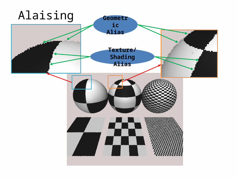
AlaisingGeometric
Alias
Texture/Shading Alias

Shadow Alaising

More Subtle Alaising Should NOT see pattern!!
Maya Scene

Aliasing in Time!
• Wagon Wheel Effect!?– Stroboscopic effect
– http://www.youtube.com/watch?v=jHS9JGkEOmA
• Or– http://www.youtube.com/watch?v=rVSh-au_9aM
Period=8 Unit
Period=7 Unit

Time/Space AnalogyColor “changes”
rapidly over space
Color “changes”slowly over space
• Many pixels to describe simple (no) transition
• In time, object moves very slowly, many frames to capture movement
• One pixel must capture many blackwhite transitions!
• One frame must capture much movement over time
• Observation: Aliasing results when …– Changes too fast for the sampling rates!

Intensity of the line
How to measure: rate of change?• Rate of Change:– Frequency!
• Frequency of images– How to measure?
• Goal:– Appreciation for
Nyquist frequency
One line of color

A little math …
• Approach:– Find mathematic representation for this simple case– Study to understand the characteristic– Generalize to discuss aliasing we observed
Assume width of 4 (T=4) Let’s say repeats every
width of 20 (W = 2*/10)

Exercise
• Plot:
T=420 (W = 2*/20)
• Independent of x (pixel position)• A series of constants according to k
• Cosine function in x (pixel position)• Adding a series cosine functions

Plotting …N = 1
N = 10
N = 20
N = 80
T=420 (W = 2*/20)
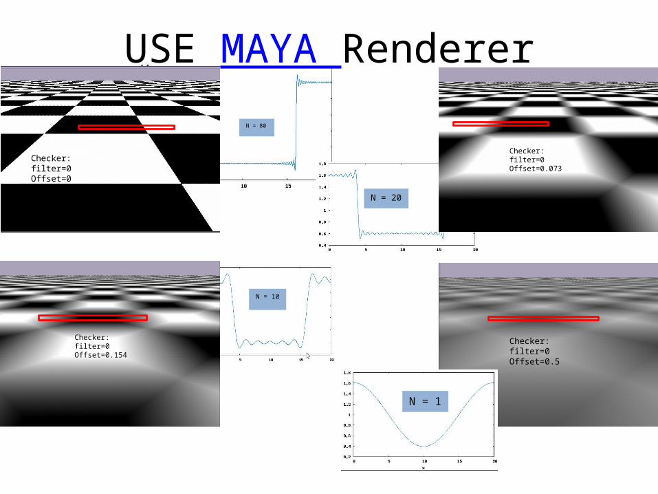
N = 10
N = 80
N = 20
USE MAYA Renderer
Checker: filter=0Offset=0
Checker: filter=0Offset=0.073
Checker: filter=0Offset=0.154
Checker: filter=0Offset=0.5
N = 1

Observation• When N is small– For each x value:
needs small number of terms– Smooth transitions
• When N gets large: – For each x value:
needs large number of terms– Sharper transitions
• N controls frequency of the cosine curves: – shape transitions: high frequency

What have we done?• Took an extremely simple part of an image:– Show how to represent with math
• Analyzed the math expression– Define: high vs. low frequency
• What we did not do:– Show: any given image (function) can be expressed
as a summation of sinusoidal functions– Term: transform an image (function) to frequency
domain (e.g., Fourier Transform)

• We have seen Square signal (function) in 1D:
• Restricting N to small numbers– corresponds to smooth the square corners– Low pass “filtering” (only keep low frequency)
• Restricting N to large numbers– Corresponds to keep only the corners– High pass filtering (only allow high frequency)– E.g., only sum terms – between 100 and 200:
Frequency of A Signal

Frequency “Domain”• Plot the size of the cosine terms of functions!• E.g., the square pulse– Can be expressed as:
Frequency domain is a plot of these terms against k …
Cosine functions: define how fast the signal will vary

Frequency Domain: Examples
FTL-SE to try out!• Try high/low pass
filtering!!• Scenes (Checker, Sine)

Frequency of an image• High Frequency:– Sharp color changes
• Low Frequency: – Smooth or no change
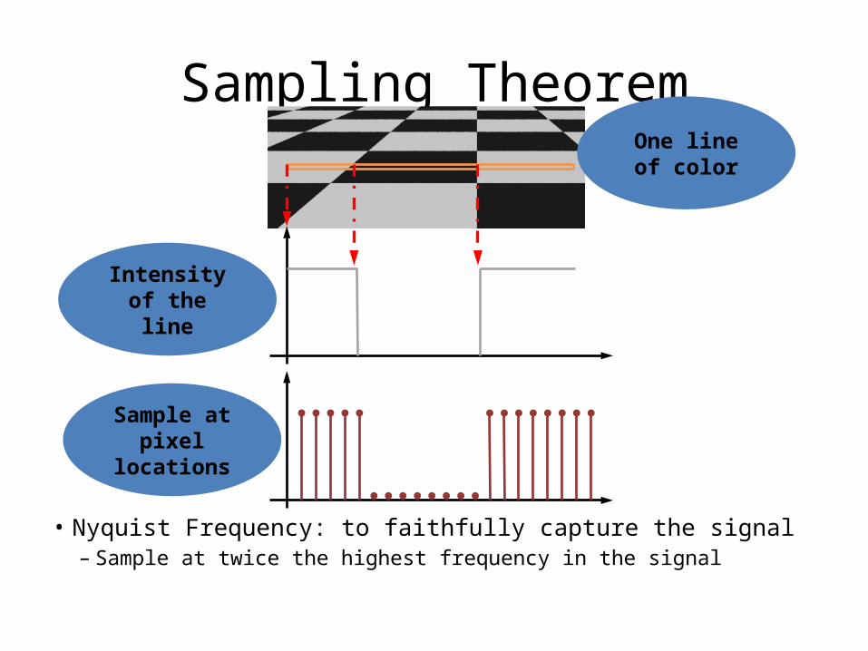
Sampling Theorem
• Nyquist Frequency: to faithfully capture the signal– Sample at twice the highest frequency in the signal
Intensity of the line
One line of color
Sample at pixel locations

Sampling Rate
• Distance between the samples: – Small High sampling rate– Large Low sampling rate
• BAD NEWS!!– Square signal (checker transition) has infinite
frequency! (N ∞ for
Sample locations
One scaneline