WP/14/2

SAMA Working Paper:

DYNAMICS OF INVESTORS’ RISK AVERSION IN EMERGING

STOCK MARKETS: EVIDENCE FROM SAUDI ARABIA

December 2014

By

Saudi Arabian Monetary Agency

The views expressed are those of the author(s) and do not necessarily reflect the

position of the Saudi Arabian Monetary Agency (SAMA) and its policies. This

Working Paper should not be reported as representing the views of SAMA.

Ayman F. Alfi

Financial Stability Division

Saudi Arabian Monetary Agency

Saudi Arabian Monetary Agency

Tapas K. Mishra

Southampton University

United Kingdom

2

Dynamics of Investors’ Risk Aversion in Emerging Stock *e from Saudi ArabiaEvidencMarkets:

Abstract

Investors’ attitude towards risk taking behavior is one of the key

determinants of financial market volatility. The attitude itself, however,

differs significantly between developed and developing markets, given the

amount of uncertainty they face with regard to market imperfection and

available information. This paper provides an in-depth study of the extent to

which risk aversion behavior in a developing financial market contributes

towards volatility. To this end, we employ a range of tests building on the

basic GARCH-M procedure, estimate the risk aversion parameter and study

its movement over time. Saudi Arabia’s financial market has been taken as

a case of empirical illustration. It is shown that the risk-aversion parameter

is time-varying and embeds information from the changing economic

environment. Moreover, we also argue that in such a market, given

characteristic volatility with respect to imperfection and incomplete

information, it is hard to predict the exact pattern of volatility.

Keywords: Emerging markets; Risk aversion; GARCH models; Kalman

filter

JEL classification: G01; G11; G17; G32

* We would like to thank Dr. Giovanni Urga from Cass Business School-London, and Prof. Sushanta K. Mallick

from The School of Business and Management – Queen Mary University of London for their constructive comments.

Author contacts: Ayman Alfi, Financial Stability Division, Saudi Arabian Monetary Agency, P. O. Box 2992 Riyadh

11169, Email: aalfi@sama.gov.sa

3

1. Introduction

During the first few years of this century, the rapid increase in

investment in the largest stock market in the Middle East (viz., the Saudi

stock market) and the dramatic losses following its collapse in 2006 raised

serious questions about investors’ perception towards risk in emerging

markets. As a consequence, both economic theory and empirical models

dealing with issues of risk aversion in financial markets developed analyses

which accounted for factors like incomplete information, imperfect markets,

and herding behavior under stochastic shocks. The broad questions that can

be asked then are:

How do risk-averse investors perceive risk?

What is the level of risk aversion in the market?

Does risk aversion evolve over time?

How may market crashes affect investors’ risk attitude?

These issues are critical to investors and policy makers in order to ensure

sound investment strategies and stable financial markets. In this paper, we

seek to understand the dynamics of risk aversion in a financial market which

is in a transitional phase and is beset with greater degrees of market

imperfection and incomplete information.

Indeed, the stability of financial systems is argued to be linked to many

factors, including stability in share prices (e.g., Granville and Mallick, 2009),

which in turn is linked to investor’s risk attitude. We intend to investigate

these issues in detail and study risk attitudes that prevail in emerging

4

financial markets. The examination of individual risk behavior has been of

interest to researchers since the mid-1940s. Friedman and Savage (1948), for

instance, provided a utility analysis of choices involving risk. They argued

that, under the law of diminishing marginal utility, utility maximization

theory is not sufficient under risk choices. If the law of diminishing marginal

utility stands, individuals should never engage in a fair gamble.

Alternatively, risky choices should be studied within the framework of

expected utility maximization. However the issue of risk aversion was

directly tackled in the 60’s when Pratt (1964) and Arrow (1971) derived

expressions for risk aversion. Arrow (1971) defines a risk averter as “one

who, starting from a position of certainty, is unwilling to take a bet which is

actuarially fair”. He showed theoretically that the coefficient of relative risk

aversion (CRRA) should be around unity

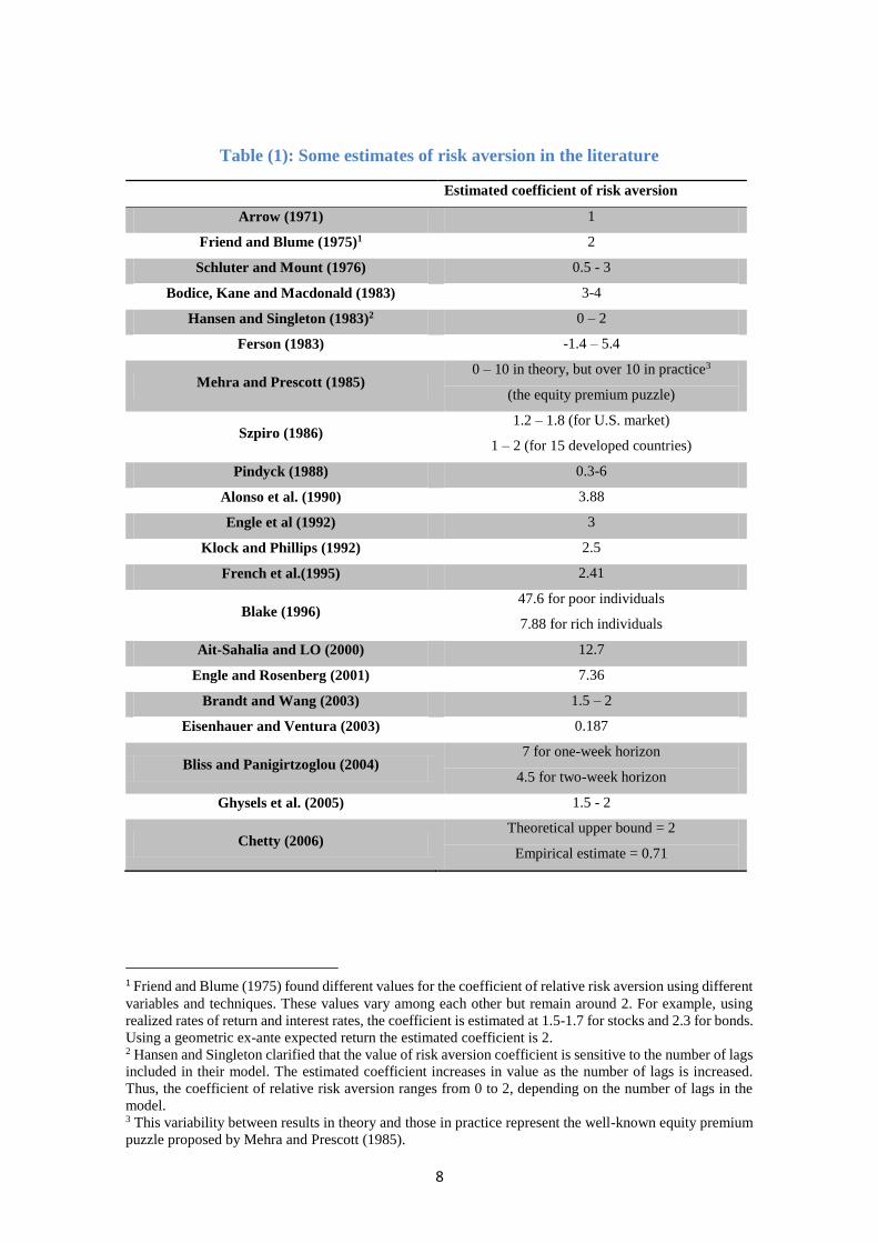
Studies have differed widely with respect to their estimates of risk

aversion (Table 1). Friend and Blume (1975) estimated the CRRA to be

between 1.5 and 1.7 for the stock market and 2.3 for the bonds market. Mehra

and Prescott (1985) argued that the CRRA should exceed 10 in order to

reconcile the equity risk premium with theoretical models. Pindyck (1988)

provided estimates of the index of relative risk aversion that ranged from 0.3

to slightly over 6. Alonso, Rubio and Tusell (1990) found that CRRA in the

Spanish stock market is 3.88. French, Schwert and Stambaugh (1995) have

estimated it to be equal to 2.41. More recently, others such as Brandt and

Wang (2003) and Ghysels et al. (2005) estimated the CRRA to range from

1.5 to 2 on average. Guo and Whitelaw (2006) estimated a coefficient of

around 5. Obviously, empirical studies have varied widely in terms of the

sign of the estimated CRRA.

5

In contrast to the studies mentioned above, some studies found a

negative return-risk relation. According to Glosten et al. (1993), the

relationship between returns and risk can take either a positive or negative

sign. Elyasiani and Mansur (1989) found a negative and significant effect of

risk aversion on return in US data. Basher et al. (2007) reached the same

result in the Bangladesh stock market. Others, such as Thomas (1995), found

no evidence of a significant effect of risk on return at all.

The coefficient of variance in the conditional mean equation is

interpreted as investors’ coefficient of relative risk aversion (Merton, 1980).

In line with Merton, Lintner (1970) states in a theorem that the market price

of risk is equivalent to the market risk aversion. Yet, empirical studies of the

conditional mean-variance relationship seem to produce conflicting

predictions in terms of the magnitude and sign of such a relationship. For

example, Elyasiani and Mansur (1998) found a negative and significant

relation while Chou (1988) reported that this relation is positive and

significant. However, according to Merton (1980), a positive relation

between expected return and risk is a reasonable assumption, although this

assumption need not always be true.

If changes in preferences or in the distribution of wealth are such that

aggregate risk aversion declines between one period and another, then higher

market risk in the one period does not need to imply a correspondingly higher

risk premium. At first glance, it would appear that risk-averse investors

should require a larger risk premium during times when the volatility of

returns increases. However, some (e.g., Glosten et al (1993) have argued that

larger risk may not necessarily imply an increasing risk premium, because

high volatility periods could coincide with times in which investors are more

capable of bearing risk. Additionally, it may be the case that investors choose

6

to increase their savings during risky periods, thus lowering the need for a

larger risk premium. Glosten et al. also argued that, if transferring income to

the future is risky and investment in risk free assets is not available, the price

of a risky asset may increase considerably, hence reducing the risk premium.

Abel (1988) claimed that, in general equilibrium, if investor’s preference is

not logarithmic, the mean-variance relationship will not necessarily be

positive.

Therefore, either a positive or negative correlation between the

conditional mean and conditional variance can be consistent with underlying

theories. Barsky (1989) provides an extensive discussion on the risk return

relationship. He makes a distinction between risk aversion and aversion to

intertemporal substitution. Barsky shows that the effect of increased equity

risk on required stock returns is ambiguous. The expression for change in

expected return with respect to change in risk contains two terms. The first

is represented by risk aversion and can be thought of as the substitution

effect. This first term takes a positive sign. Increased riskiness of the capital

asset exerts pressure toward greater first-period consumption in order to

avoid the risk, causing a corresponding fall in the notional demand for

equities. Since, in equilibrium, the representative consumer must hold his/her

share of the fixed stock supply of capital, this tends to raise required returns.

On the other hand, the second term, under decreasing absolute risk aversion,

takes a negative sign and can be thought of as a precautionary saving effect.

Increased risk raises the prospect of very low consumption in the second

period, increasing asset demands and exerting downward pressure on

required returns.

7

Thus, an increase in uncertainty can result in either a rise or fall in the

required return to equity, depending on which effect dominates. In the case

of constant risk aversion, equilibrium expected return on capital rises with

increased uncertainty if and only if the CRRA is less than unity. Thereby,

the effect of uncertainty is a function of risk aversion and the intertemporal

rate of substitution. The degree of substitutability between first and second

period consumption determines the sign of the risk-return relationship, while

the risk aversion help determining the magnitude of the effect but not its sign.

This conclusion by Barsky will be adopted in our interpretation of the results

acquired here.

The rest of the paper is structured as follows. The model is set up and

the coefficient of risk aversion is derived in section 2. Section 3 discusses

the data and section 4 provides our empirical analysis and results. Section 5

discusses the policy implications of our results and, finally, section 6

concludes.

8

Table (1): Some estimates of risk aversion in the literature

Estimated coefficient of risk aversion

Arrow (1971) 1

Friend and Blume (1975)1 2

Schluter and Mount (1976) 0.5 - 3

Bodice, Kane and Macdonald (1983) 3-4

Hansen and Singleton (1983)2 0 – 2

Ferson (1983) -1.4 – 5.4

Mehra and Prescott (1985) 0 – 10 in theory, but over 10 in practice3

(the equity premium puzzle)

Szpiro (1986) 1.2 – 1.8 (for U.S. market)

1 – 2 (for 15 developed countries)

Pindyck (1988) 0.3-6

Alonso et al. (1990) 3.88

Engle et al (1992) 3

Klock and Phillips (1992) 2.5

French et al.(1995) 2.41

Blake (1996) 47.6 for poor individuals

7.88 for rich individuals

Ait-Sahalia and LO (2000) 12.7

Engle and Rosenberg (2001) 7.36

Brandt and Wang (2003) 1.5 – 2

Eisenhauer and Ventura (2003) 0.187

Bliss and Panigirtzoglou (2004) 7 for one-week horizon

4.5 for two-week horizon

Ghysels et al. (2005) 1.5 - 2

Chetty (2006) Theoretical upper bound = 2

Empirical estimate = 0.71

1 Friend and Blume (1975) found different values for the coefficient of relative risk aversion using different

variables and techniques. These values vary among each other but remain around 2. For example, using

realized rates of return and interest rates, the coefficient is estimated at 1.5-1.7 for stocks and 2.3 for bonds.

Using a geometric ex-ante expected return the estimated coefficient is 2. 2 Hansen and Singleton clarified that the value of risk aversion coefficient is sensitive to the number of lags

included in their model. The estimated coefficient increases in value as the number of lags is increased.

Thus, the coefficient of relative risk aversion ranges from 0 to 2, depending on the number of lags in the

model. 3 This variability between results in theory and those in practice represent the well-known equity premium

puzzle proposed by Mehra and Prescott (1985).

9

2. Model Setup

There are several factors that motivate the use of GARCH models in

the analysis procedure. As often found in the financial literature, the

distribution of stock returns is leptokurtic. Hence, standard linear regression

cannot capture the fat tail and heteroscedasticity properties of the data. Also,

in contrast to the standard time series regression models, the ARCH model

proposed by Engle (1982) allows the variance of the errors to change over

time. Additionally, the different types of GARCH models allow estimation

of volatility without assuming a functional form of volatility that depends on

returns, unlike other time series models. Moreover, with the shortage of high

frequency return data for emerging financial markets, it is difficult to model

daily volatility using standard time series models (e.g. ARIMA models).

Even if weekly returns are used, this will come at the cost of losing

observations, resulting in fewer degrees of freedom. This is not a problem in

a GARCH framework as it uses an iterative process in estimating daily

volatility.

Bollerslev (1986) proposed a generalization of the Engle’s ARCH

model in what is now known as a GARCH model. The GARCH process

allows for a lag structure for the variance and models the conditional

variance as a function of prior periods’ squared errors and conditional

variances. One of the major advantages of GARCH models, which make

them very popular in financial data analysis, is that they are capable of

capturing the tendency for volatility clustering in the data. For example, large

(small) changes in stock returns are most likely to be followed by large

(small) stock returns in the next period. Engle et al. (1987) extended the

GARCH structure to explicitly model the conditional mean of the data as a

function of its conditional variance, in what is known as the GARCH in mean

10

or GARCH-M model. This approach allows for assessing the relationship

between return and risk in financial data and for taking into account the

leptokurtosis and volatility clustering feature, especially in emerging

markets data. The GARCH-M(p,q) model is represented as follows:

𝑅𝑡 = 𝜇 + 𝛿𝜎𝑡2 + 𝜖𝑡 (1)

𝜎𝑡2 = 𝜔 + ∑ 𝛼𝑖휀𝑡−𝑖

2𝑞𝑖=1 + ∑ 𝛽𝑖𝜎𝑡−𝑖

2𝑞𝑖=1 (2)

where 𝑅𝑡 and 𝜎𝑡2 are the conditional return and variance at time t.

The obvious limitations of the GARCH model can be solved by

adopting the EGARCH model as was proposed by Nelson (1991). Basically,

Nelson proposed to relax the non-negativity constraints assumed in the

original GARCH specification to allow for asymmetry in conditional

variance. Nelson included a leverage effect in the variance equation and

applied the log of the conditional variance rather than the conditional

variance itself. Using the log implies that the leverage effect is exponential,

rather than quadratic and the forecasts of the conditional variance are

guaranteed to be non-negative. The variance equation for the EGARCH(1,1)

model is specified as follows:

ln(𝜎𝑡2) = 𝜔 + 𝛽 ln(𝜎𝑡−1

2 ) + 𝛼1 |𝜀𝑡−1

𝜎𝑡−1| + 𝛾

𝜀𝑡−1

𝜎𝑡−1 (3)

EGARCH has several advantages over the basic GARCH model. First,

using the natural logarithm in the variance equation ensures that the

11

conditional variance, , is always non-negative, even if the parameters are

negative. Thus, there is no need to artificially impose any non-negativity

constraints on the model’s parameters. Second, it allows for asymmetry in

response to volatility. The standard GARCH model does not distinguish

between positive and negative shocks to volatility. Since it is a function of

the squared lagged error, the conditional variance in the basic GARCH

model is a function of the magnitudes of the lagged residuals but not their

signs. Accordingly, it assumes that the response to negative shocks is just the

same as the response to positive shocks. It has been argued, however, that a

negative shock to financial time series causes volatility to rise by more than

a positive shock of the same magnitude, a phenomenon known as the

“leverage effect”. EGARCH accounts for asymmetric shock response by

including the last term in the equation above4.

2.1 Risk Aversion and Utility Functions

To reconcile our empirical models with the underlying theory in

finance, we start by showing how investors’ aggregate risk-return is linked

to his/her utility function where the latter is drawn from consumer preference

theory. By utilizing the theoretical underpinning of the derived empirical

model (as will be described in the next section), we also shed light on the

important aspects of risk aversion and its interrelationships with market

structure. As argued before, the environment in which investors are adopting

4 It is worth mentioning that the original formulation for EGARCH model assumed a Generalized

Error Distribution (GED), which is a broad family of distributions that can be used for many types or series.

Nevertheless, rather than using GED, we stick to the conditional normal error assumption originally

suggested by Engle (1982).

12

strategies of risk aversion or risk taking behavior has enormous influence on

their psychology. For instance, under a volatile market and incomplete

information, investors may depict ‘herding’ behavior, as they would not be

able to predict the exact pattern of the economy at period t+1. In this case,

they may follow a market leader. Similarly, if the market is relatively less

volatile and information dissemination is more or less perfect, then investors

may wish to take some risks and play strategic games in relation with other

investors.

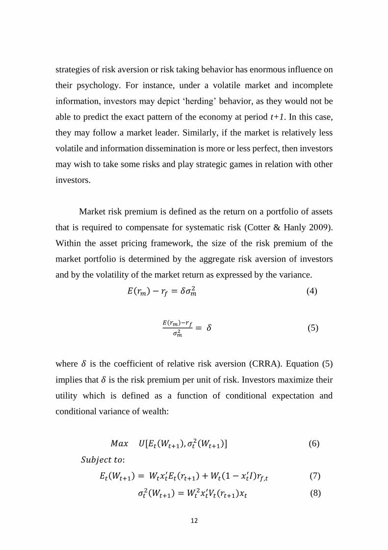
Market risk premium is defined as the return on a portfolio of assets

that is required to compensate for systematic risk (Cotter & Hanly 2098).

Within the asset pricing framework, the size of the risk premium of the

market portfolio is determined by the aggregate risk aversion of investors

and by the volatility of the market return as expressed by the variance.

𝐸(𝑟𝑚) − 𝑟𝑓 = 𝛿𝜎𝑚2 (4)

𝐸(𝑟𝑚)−𝑟𝑓

𝜎𝑚2 = 𝛿 (5)

where 𝛿 is the coefficient of relative risk aversion (CRRA). Equation (5)

implies that 𝛿 is the risk premium per unit of risk. Investors maximize their

utility which is defined as a function of conditional expectation and

conditional variance of wealth:

𝑀𝑎𝑥 𝑈[𝐸𝑡(𝑊𝑡+1), 𝜎𝑡2(𝑊𝑡+1)] (6)

𝑆𝑢𝑏𝑗𝑒𝑐𝑡 𝑡𝑜:

𝐸𝑡(𝑊𝑡+1) = 𝑊𝑡𝑥𝑡′𝐸𝑡(𝑟𝑡+1) + 𝑊𝑡(1 − 𝑥𝑡

′𝐼)𝑟𝑓,𝑡 (7)

𝜎𝑡2(𝑊𝑡+1) = 𝑊𝑡

2𝑥𝑡′𝑉𝑡(𝑟𝑡+1)𝑥𝑡 (8)

13

where W represents investor’s wealth, x is a vector of investment shares in

each risky asset, 𝐸𝑡(𝑟𝑡+1) and 𝑉𝑡(𝑟𝑡+1) are the conditional expected return

and variance-covariance matrix of asset returns, respectively. I is a unit

vector and 𝑟𝑓,𝑡 is the risk free return.

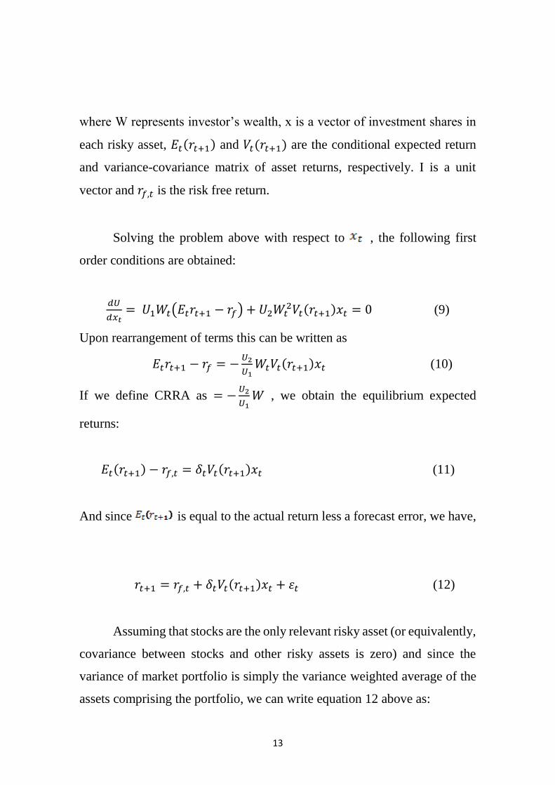
Solving the problem above with respect to , the following first

order conditions are obtained:

𝑑𝑈

𝑑𝑥𝑡= 𝑈1𝑊𝑡(𝐸𝑡𝑟𝑡+1 − 𝑟𝑓) + 𝑈2𝑊𝑡

2𝑉𝑡(𝑟𝑡+1)𝑥𝑡 = 0 (9)

Upon rearrangement of terms this can be written as

𝐸𝑡𝑟𝑡+1 − 𝑟𝑓 = −𝑈2

𝑈1𝑊𝑡𝑉𝑡(𝑟𝑡+1)𝑥𝑡 (10)

If we define CRRA as = −𝑈2

𝑈1𝑊 , we obtain the equilibrium expected

returns:

𝐸𝑡(𝑟𝑡+1) − 𝑟𝑓,𝑡 = 𝛿𝑡𝑉𝑡(𝑟𝑡+1)𝑥𝑡 (11)

And since is equal to the actual return less a forecast error, we have,

𝑟𝑡+1 = 𝑟𝑓,𝑡 + 𝛿𝑡𝑉𝑡(𝑟𝑡+1)𝑥𝑡 + 휀𝑡 (12)

Assuming that stocks are the only relevant risky asset (or equivalently,

covariance between stocks and other risky assets is zero) and since the

variance of market portfolio is simply the variance weighted average of the

assets comprising the portfolio, we can write equation 12 above as:

14

𝑟𝑠,𝑡 = 𝑟𝑓,𝑡 + 𝛿𝑡𝜎𝑠,𝑡2 + 휀𝑡 (13)

where 𝑟𝑠,𝑡 is return on the stock index, and 𝜎𝑠,𝑡2 is the variance of stock index

returns. Therefore, a rational, utility maximizing consumer/investor will

regard the excess return on his/her portfolio as a function of risk.

3. Data

For our empirical analysis, we use daily closing prices from the Saudi

Arabian Stock Exchange. The data are obtained from the Saudi Stock

Exchange (Tadawul) and constitutes of 2161 observations on the Tadawul

All Share Index (TASI) prices. The data covers the period from January 1st,

2003 to December 31st, 2010. The sample is subdivided into two periods:

January 1st, 2003 to Feb 28th, 2006 with 943 observations, and March 1st,

2006 to December 31st, 2010 with 1218 observations. The estimation

process covered the two periods in addition to the full sample size. The

subdivision of the sample is necessary to investigate whether investor’s

attitude towards risk has changed after the market crash in February 26th,

2006, or not. Daily TASI return series are generated from the index closing

prices. Index return at time “t” is calculated as the difference between the

natural logarithm of its price at time “t” and its price for the day before (i.e.

at time “t-1”).

4. Empirical Analysis

4.1. Model with Fixed Risk Aversion

Within the model of capital market equilibrium, the excess return on

investing in risky asset is modelled as a function of the standard deviation of

15

that return. In financial terms, the risk premium, defined as the excess return

of an investment, is approximately proportional to the amount of risk being

born by investors where risk is measured by the volatility of return in the

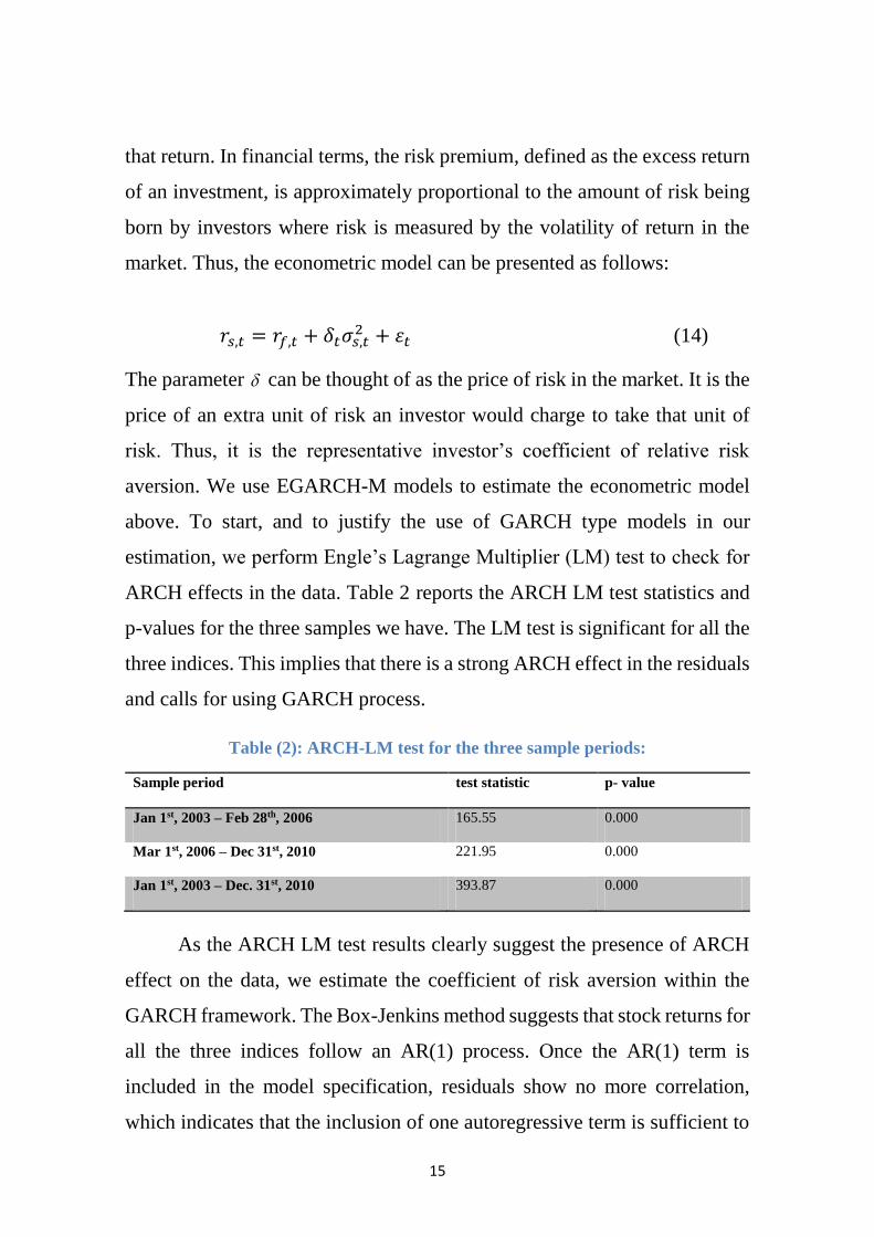
market. Thus, the econometric model can be presented as follows:

𝑟𝑠,𝑡 = 𝑟𝑓,𝑡 + 𝛿𝑡𝜎𝑠,𝑡2 + 휀𝑡 (14)

The parameter can be thought of as the price of risk in the market. It is the

price of an extra unit of risk an investor would charge to take that unit of

risk. Thus, it is the representative investor’s coefficient of relative risk

aversion. We use EGARCH-M models to estimate the econometric model

above. To start, and to justify the use of GARCH type models in our

estimation, we perform Engle’s Lagrange Multiplier (LM) test to check for

ARCH effects in the data. Table 2 reports the ARCH LM test statistics and

p-values for the three samples we have. The LM test is significant for all the

three indices. This implies that there is a strong ARCH effect in the residuals

and calls for using GARCH process.

Table (2): ARCH-LM test for the three sample periods:

Sample period test statistic p- value

Jan 1st, 2003 – Feb 28th, 2006 165.55 0.000

Mar 1st, 2006 – Dec 31st, 2010 221.95 0.000

Jan 1st, 2003 – Dec. 31st, 2010 393.87 0.000

As the ARCH LM test results clearly suggest the presence of ARCH

effect on the data, we estimate the coefficient of risk aversion within the

GARCH framework. The Box-Jenkins method suggests that stock returns for

all the three indices follow an AR(1) process. Once the AR(1) term is

included in the model specification, residuals show no more correlation,

which indicates that the inclusion of one autoregressive term is sufficient to

16

capture autocorrelation in the data. Therefore, to estimate the coefficient of

risk aversion, we fit an AR(1)-GARCH(1,1)-M model,

𝑅𝑡 = 𝜇 + 𝜑𝑅𝑡−1 + 𝛿𝜎𝑡2 + 𝜖𝑡 (15)

𝜎𝑡2 = 𝜔 + 𝛼휀𝑡−1

2 + 𝛽𝜎𝑡−12 (16)

where 𝑅𝑡 denotes stock return at time “t”, 𝜖𝑡 is the prediction error assumed

to be normally distributed with mean zero and conditional variance 𝜎𝑡2 that

is changing each day. 𝛿 denotes investors’ coefficient of risk aversion. Note

that the time subscript “t” drops out as we assume a constant risk aversion

over time. Additionally, the restrictions 𝛼 + 𝛽 ≥ 1 for i = 0, 1 and 2 is

imposed to ensure a positive conditional variance, 𝜎𝑡2.

As demonstrated in Engle and Bollerslev (1986), Chou (1988),

Bollerslev et al. (1992), the persistence of the shocks to volatility depends

on the sum of 𝛼 + 𝛽. If 𝛼 + 𝛽 > 1, the effect of shocks on volatility tends

to vanish over time. On the other hand, 𝛼 + 𝛽 > 1 implies increasing, or

indefinite volatility persistence. As proposed by Poterba and Summers

(1987), a significant impact of volatility on stock prices requires the

persistence of shock to volatility for a long time.

We also extend our estimation methodology by employing an AR(1)-

EGARCH(1,1)-M model. This model extension provides a robust

estimation, as it allows for asymmetric response to volatility. Table 3

presents the empirical results from AR(1)-GARCH(1,1)-M and AR(1)-

EGARCH(1,1)-M models for the three periods. From the EGARCH model

the estimated price of risk for the first period is 3.49, but appears to be

insignificant implying that risk was not a primary determinant factor for

returns before the market crash in February 2006.

17

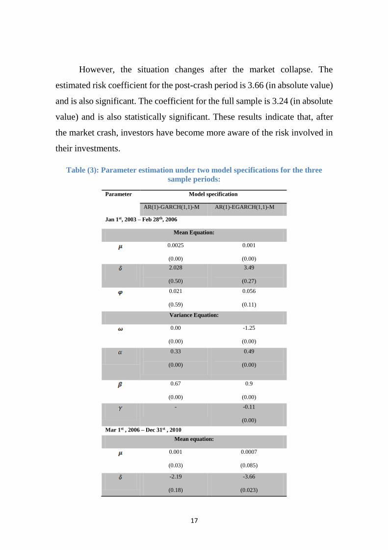
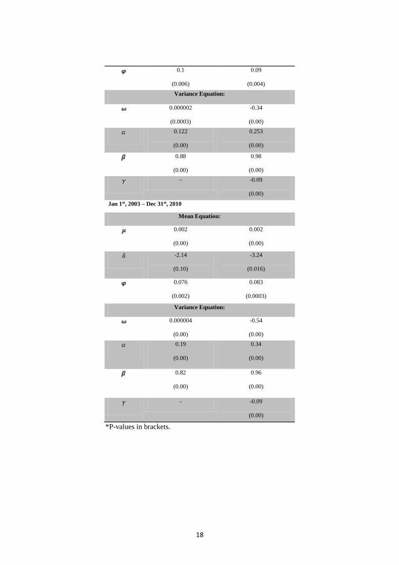
However, the situation changes after the market collapse. The

estimated risk coefficient for the post-crash period is 3.66 (in absolute value)

and is also significant. The coefficient for the full sample is 3.24 (in absolute

value) and is also statistically significant. These results indicate that, after

the market crash, investors have become more aware of the risk involved in

their investments.

Table (3): Parameter estimation under two model specifications for the three

sample periods:

Parameter Model specification

AR(1)-GARCH(1,1)-M AR(1)-EGARCH(1,1)-M

Jan 1st, 2003 – Feb 28th, 2006

Mean Equation:

0.0025

(0.00)

0.001

(0.00)

2.028

(0.50)

3.49

(0.27)

0.021

(0.59)

0.056

(0.11)

Variance Equation:

0.00

(0.00)

-1.25

(0.00)

0.33

(0.00)

0.49

(0.00)

0.67

(0.00)

0.9

(0.00)

- -0.11

(0.00)

Mar 1st , 2006 – Dec 31st , 2010

Mar 1st, 2006 – Dec 31st, 2010 Mean equation:

0.001

(0.03)

0.0007

(0.085)

-2.19

(0.18)

-3.66

(0.023)

18

0.1

(0.006)

0.09

(0.004)

Variance Equation:

0.000002

(0.0003)

-0.34

(0.00)

0.122

(0.00)

0.253

(0.00)

0.88

(0.00)

0.98

(0.00)

- -0.09

(0.00)

Jan 1st, 2003 – Dec 31st, 2010

Mean Equation:

0.002

(0.00)

0.002

(0.00)

-2.14

(0.10)

-3.24

(0.016)

0.076

(0.002)

0.083

(0.0003)

Variance Equation:

0.000004

(0.00)

-0.54

(0.00)

0.19

(0.00)

0.34

(0.00)

0.82

(0.00)

0.96

(0.00)

- -0.09

(0.00)

*P-values in brackets.

19

4.2. Models with Time Varying Risk Aversion

In the extant literature, there is profound evidence which suggests that

risk aversion is time varying (e.g., Campbell and Cochrane (1999)). Drawing

on the main implications in this regard from the recent literature, we employ

the GARCH-M framework in an attempt to estimate the time-varying risk

parameter for equity market participants. Although a standard GARCH

model assumes time varying risk represented by volatility, it also assumes a

constant coefficient of risk aversion (i.e., constant 𝛿) across time. This

implies that an investor’s attitude towards risk does not change over time

even if market characteristics change. This assumption has been questioned

by many researchers. Chou, Engle and Kane (1992), Li (2007), Ahn and

Shrestha (2009) have all argued that the price of risk is time-varying. Indeed,

many studies have shown different estimated values for the price of risk

across different sample periods. French, Schwert, and Stambaugh (1987), for

example, reported different estimates for the parameter of risk across the

different subsamples they used. Their estimates ranged from 1.5 for the

period 1928-1952 to 7.2 for the period 1952-1984. In fact, the different

estimates of risk aversion we find between the two sub-samples give initial

evidence that risk aversion has changed over time. Thus, we next propose

modeling this time variation in risk aversion.

4.2.1. Rolling Sample Estimation

To examine the behavior of the coefficient of risk aversion over time,

we perform a rolling sample regression. The AR(1)-GARCH(1,1)-M

coefficients are estimated for each day in the sample. The estimation

procedure is to estimate each day’s risk aversion coefficient by rolling a

sample of 400 observations. We start by taking a window size that contains

the first 400 observations, estimating the coefficient for the observation

20

number 401, and then rolling the sample one step ahead to estimate the

observation 402, and so on. The estimation procedure yields a series of

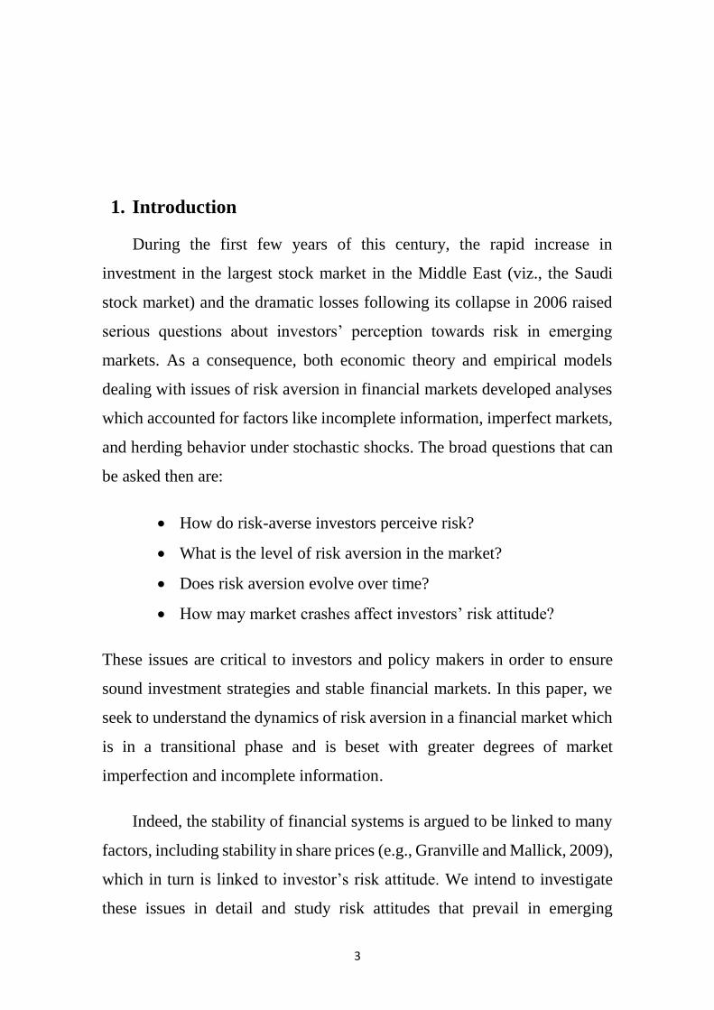
estimated risk/return coefficients. Figure 1 illustrates the daily movement of

investor’s risk aversion through the sample period excluding the first 400

observations, which account for about a two-year period.

Figure 1: Rolling regression for the movement in the price of risk (2003 - 2010)

The risk/return coefficient appears to be strongly varying during the

sample period, ranging from around -6 to 8. It is interesting to notice how

the risk/return relation dramatically changed around the observation number

1000, which coincides with the time when the equity market collapsed on

February 26th, 2006. This dramatic change gives a preliminary view on how

investors changed their perspective on pricing the risk they bear.

4.2.2. Estimation Using the Kalman Filter

The rolling sample estimation, however, has its drawbacks. First, the

estimation still assumes a fixed parameter during the window sample size of

400 observations. Additionally, the rolling sample results show large

changes in the parameter’s estimate which are unlikely to occur on a daily

basis. And last but not least, using the Kalman filter provides a much more

robust estimation method as it incorporates the arrival of new information in

-6

-4

-2

0

2

4

6

8

10

250 500 750 1000 1250 1500 1750 2000

RESULTS

21

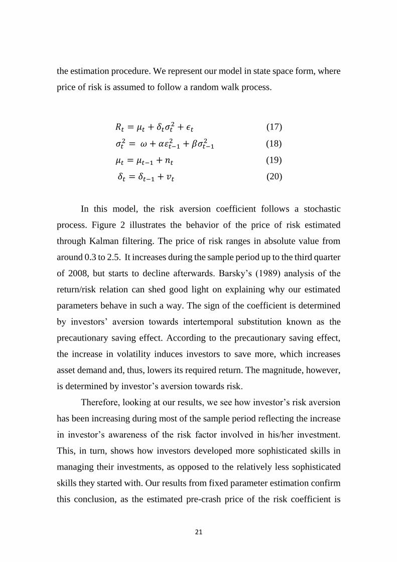
the estimation procedure. We represent our model in state space form, where

price of risk is assumed to follow a random walk process.

𝑅𝑡 = 𝜇𝑡 + 𝛿𝑡𝜎𝑡2 + 𝜖𝑡 (17)

𝜎𝑡2 = 𝜔 + 𝛼휀𝑡−1

2 + 𝛽𝜎𝑡−12 (18)

𝜇𝑡 = 𝜇𝑡−1 + 𝑛𝑡 (19)

𝛿𝑡 = 𝛿𝑡−1 + 𝑣𝑡 (20)

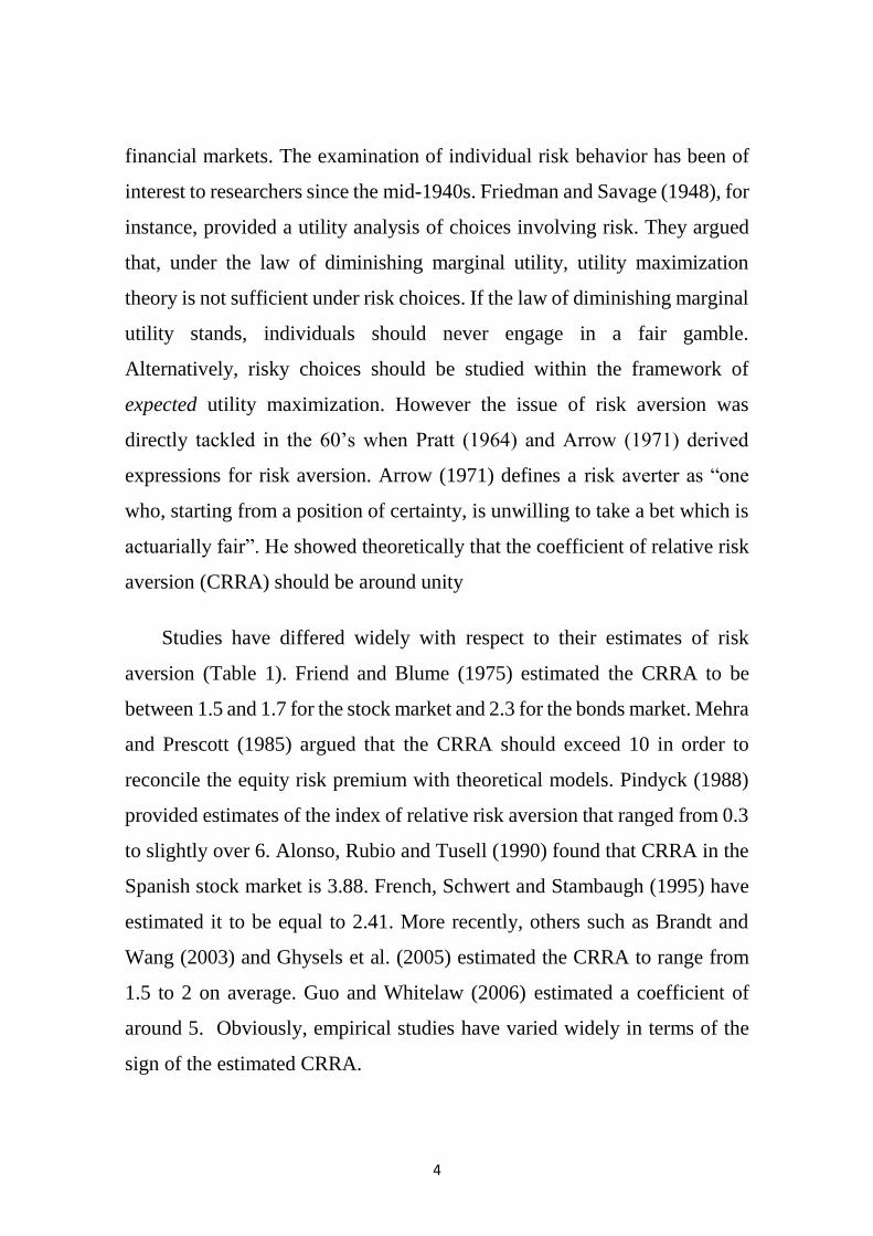
In this model, the risk aversion coefficient follows a stochastic

process. Figure 2 illustrates the behavior of the price of risk estimated

through Kalman filtering. The price of risk ranges in absolute value from

around 0.3 to 2.5. It increases during the sample period up to the third quarter

of 2008, but starts to decline afterwards. Barsky’s (1989) analysis of the

return/risk relation can shed good light on explaining why our estimated

parameters behave in such a way. The sign of the coefficient is determined

by investors’ aversion towards intertemporal substitution known as the

precautionary saving effect. According to the precautionary saving effect,

the increase in volatility induces investors to save more, which increases

asset demand and, thus, lowers its required return. The magnitude, however,

is determined by investor’s aversion towards risk.

Therefore, looking at our results, we see how investor’s risk aversion

has been increasing during most of the sample period reflecting the increase

in investor’s awareness of the risk factor involved in his/her investment.

This, in turn, shows how investors developed more sophisticated skills in

managing their investments, as opposed to the relatively less sophisticated

skills they started with. Our results from fixed parameter estimation confirm

this conclusion, as the estimated pre-crash price of the risk coefficient is

22

insignificant, indicating that risk was not a primary factor in investor’s

decision-making process. This result is in line with other results found by

other studies that conclude there is an insignificant risk-return relationship

in emerging markets (see for example, Patel and Patel, 2011, Kovacic, 2008).

As time goes on, however, the coefficient becomes more and more

significant, especially during the post-crash period.

These findings provide support towards the existence of herding

behavior in the market. Avery and Zemsky (1998), show that the level of

uncertainty in imperfect markets is positively related to “short run” herding

behavior. Thus, in an emerging market that is characterized by market

imperfection, and with our findings of increasing risk aversion, Saudi

investors are tempted to react in a herding behavior to shocks of either signs

in the market. This can be seen in the Saudi market bubble and collapse in

2006. An increase in risk aversion coupled with market imperfection led

investors to enter the market in large groups, causing a bubble. However,

once the major investors foresaw the riskiness of their investments due to

speculative behavior, they started exiting the market. This market exit again

led to a herding reaction by other investors, which in turn led to the collapse

in February 2006.

23

Figure 2: Kalman filter estimation for price of risk

5. Policy Implications

These findings have important implications for risk analysis. First,

they provide supporting evidence that risk aversion is time variant. This

evidence is new for an emerging market. Second, they explain the dynamic

nature of risk aversion and investors’ risk perception during financial crises.

Third, the results can form a guideline to regulators and central banks. A

clear understanding of investors’ risk preference is vital for central banks in

order to set appropriate monetary policy that builds central bank credibility

and eliminates macroeconomic ambiguity. To illustrate this point further,

consider the Japanese liquidity trap. Even though the Japanese central bank

has cut interest rates down to its zero lower bound, investors are still reluctant

to invest and are holding onto their money. This can be attributed to high

levels of risk aversion within the Japanese economy, which led banks to keep

the cash in their vaults in fear of bank runs, and caused investors to prefer

holding the cash as a liquid asset to protect themselves against the uncertain

future. This liquidity trap has limited the central bank’s ability to stimulate

the economy which weakened its credibility among economic agents. This

credibility is, as argued by Granville and Mallick (2009), crucial to ensure

stability in financial markets. Furthermore, prospective future research can

be built upon these findings to study investors’ reaction towards any

price of risk

2003 2004 2005 2006 2007 2008 2009 2010-2.50

-2.25

-2.00

-1.75

-1.50

-1.25

-1.00

-0.75

-0.50

-0.25

24

announced structural changes in imperfect and incomplete markets other

than the Saudi Stock Exchange.

Investors’ risk aversion has its implications for macroeconomic

policies. Governments that plan to expand their fiscal policies must be fully

aware of the level of risk aversion that prevails domestically. Fiscal

expansions are normally financed through relying on the credit market where

governments can sell their bonds. If aggregate risk aversion is at high levels,

governments may find it difficult to sell their bonds to finance their fiscal

expansion plans. Consequently, they will have to go through one of two

costly channels to acquire the fund needed. The first is to offer high yields

on their bonds to attract the highly risk-averse investors in the domestic

market. This may impose a downward pressure on their bond prices leading

to some undesirable consequences on the financial system and the real

economy putting fiscal sustainability at risk. The other channel is to turn to

the international credit market, which is a riskier alternative and more

restrictive. Therefore, it is important that policy makers be aware of the

prevailing level of risk aversion in the market and ensure that it is kept within

a sustainable level.

Last but not least, the results can be generalized to provide policy

implications to hypothetical situations that may occur in other markets that

share similar characteristics. For instance, as China and Saudi Arabia share

similar monetary policy arrangements and are export-driven economies but

differ only in the restriction on capital flow, our economic inference can

provide a good guide to Chinese policy makers on how the market may

behave if their capital flow restriction were relaxed.

25

6. Conclusion

There are few studies that have attempted to explain the behavior of

stock returns in Saudi Arabia. However, to the best of our knowledge, none

has related the movement in return’s to investor’s behavior towards financial

risk. In this paper, we have studied the effect of investor’s price of risk in the

stock market of Saudi Arabia. Our data consisted of two periods: a pre-

market crash and a post-market crash period. We started our analysis by

assuming a fixed price of risk over time. We found that, in an EGARCH-M

model specification, risk did not have a significant effect on return for the

pre-crash period. This indicates that investors, during that period, did not

consider risk to be a major factor for their required return. Yet, the situation

changes after the market collapse on February 26, 2006, after which the price

of risk becomes statistically significant and investors become more risk

avert. When relaxing the assumption of constant risk aversion over time,

these results were confirmed. The price of risk increases in absolute value as

time goes on, except for the last year in the sample, where volatility seemed

to stabilize relatively.

This result shows how investors have become more aware of the risk

involved in their investments as time goes on. These results have some

significant implications for policy makers. First, they emphasize the

importance of transparent information in the financial system. Authorities

should make sure that all information is available for investors to allow them

to account for any possible risk they may encounter in their investments and

reduce the possibility of herding behavior. They also should put emphasis on

educating investors in the risk prospects of the investment and how to

account for risk when making investments. Knowledge of some risk analysis

tools such as portfolio diversification will ensure lowering volatility and thus

26

stabilize the financial market. Additionally, the results will help market

legislators in their mission of keeping the market stable and under control.

Additionally, understanding investors’ behavior towards risk can help those

legislators implement effective laws to curb any aggressive behavior from

the investor side. It also helps understand the implications and cost of

introducing new macroeconomic policies such as fiscal expansions.

Finally, the results have their implications on policy maker decisions in

developing economies that face the same circumstances as Saudi Arabia.

Having an economy that is export driven and a pegged currency exchange

rate to the dollar makes Saudi Arabia a good case study for other emerging

countries in the region. GCC countries can be a good example as well. They

share similar aspects with Saudi Arabia when it comes to the level of market

development, monetary policy and dependence on exports. The major

difference though is the variation in the level of capital flow control. So, for

policy makers or researchers, one can draw a conclusion of the effect of

changing the restrictions on capital flow in GCC countries on their stock

markets and financial systems by considering a case study such as the one at

hand.

27

References

Abel, A. B. (1988). "Stock Prices under Time-Varying Dividend Risk:: An

Exact Solution in an Infinite-Horizon General Equilibrium Model."

Journal of Monetary Economics 22(3): 375-393.

Ahn, S. and K. Shrestha (2009). "Estimation of Market Risk Premium for

Japan." Enterprise Risk Management 1(1).

Alonso, A., G. Rubio, et al. (1990). "Asset Pricing and Risk Aversion in the

Spanish Stock Market." Journal of Banking & Finance 14(2-3): 351-

369.

Avery, C. and P. Zemsky (1998). "Multidimensional Uncertainty and Herd

Behavior in Financial Markets." The American Economic Review:

88(4): 724-748.

Barsky, R. B. (1989). "Why Don't the Prices of Stocks and Bonds Move

Together?" The American Economic Review 79(5): 1132-1145.

Basher, S. A., M. K. Hassan, et al. (2007). "Time-Varying Volatility and

Equity Returns in Bangladesh Stock Market." Applied Financial

Economics 17(17): 1393-1407.

Bollerslev, T. (1986). "Generalized Autoregressive Conditional

Heteroskedasticity." Journal of Econometrics 31(3): 307-327.

Bollerslev, T., R. Y. Chou, et al. (1992). "ARCH Modeling in Finance: A

Review of the Theory and Empirical Evidence." Journal of

Econometrics 52(1-2): 5-59.

Bollerslev, T. and J. M. Wooldridge (1992). "Quasi-Maximum Likelihood

Estimation and Inference in Dynamic Models with Time-Varying

Covariances." Econometric Reviews 11(2): 143-172.

28

Brandt, M. W. and K. Q. Wang "Time-Varying Risk Aversion and

Unexpected Inflation." Journal of Monetary Economics, Vol. 50,

2003.

Campbell, John Â. Y. and John Â. H. Cochrane (1999). "By Force of Habit:

A Consumption Based Explanation of Aggregate Stock Market

Behavior." The Journal of Political Economy 107(2): 205-251.

Chou, R., R. F. Engle, et al. (1992). "Measuring Risk Aversion from Excess

Returns on a Stock Index." Journal of Econometrics 52(1-2): 201-224.

Chou, R. Y. (1988). "Volatility Persistence and Stock Valuations: Some

Empirical Evidence Using GARCH." Journal of Applied

Econometrics 3(4): 279-294.

Cotter, J. and J. Hanly (2009). "Time-Varying Risk Aversion: An

Application to Energy Hedging." Energy Economics 32(2): 432-441.

Elyasiani, E. and I. Mansur (1998). "Sensitivity of the Bank Stock Returns

Distribution to Changes in the Level and Volatility of Interest Rate: A

GARCH-M Model." Journal of Banking & Finance 22(5): 535-563.

Engle, R. (1982). "Autoregressive Conditional Heteroskedasticity with

Estimates of the Variance of United Kingdom Inflation."

Econometrica: Journal of the Econometric Society 50(4): 987-1007.

Engle, R. F. and T. Bollerslev (1986). "Modelling the Persistence of

Conditional Variances." Econometric Reviews 5(1): 1 - 50.

Engle, R. F., D. M. Lilien, et al. (1987). "Estimating Time Varying Risk

Premia in the Term Structure: The Arch-M Model." Econometrica

55(2): 391-407.

French, K. R., G. W. Schwert, et al. (1995). "Expected Stock Returns and

Volatility." ARCH: Selected Readings: 61.

29

Friedman, M. and L. J. Savage (1948). "The Utility Analysis of Choices

Involving Risk." Journal of Political Economy 56(4): 279.

Friend, I. and M. E. Blume (1975). "The Demand for Risky Assets." The

American Economic Review 65(5): 900-922.

Ghysels, E., P. Santa-Clara, et al. (2005). "There is a Risk-Return Trade-Off

After All." Journal of Financial Economics 76(3): 509-548.

Glosten, L. R., R. Jagannathan, et al. (1993). "On the Relation between the

Expected Value and the Volatility of the Nominal Excess Return on

Stocks." The Journal of Finance 48(5): 1779-1801.

Granville, B. and S. Mallick (2009). "Monetary and Financial Stability in the

Euro Area: Pro-Cyclicality versus Trade-Off." Journal of

International Financial Markets, Institutions and Money 19(4): 662-

674.

Kovačić, Z. (2008). "Forecasting Volatility: Evidence from the Macedonian

Stock Exchange." International Research Journal of Finance and

Economics (18).

Li, G. (2007). "Time-Varying Risk Aversion and Asset Prices." Journal of

Banking & Finance 31(1): 243-257.

Lintner, J. (1970). "The Market Price of Risk, Size of Market and Investor's

Risk Aversion." The Review of Economics and Statistics 52(1): 87-99.

Mehra, R. and E. C. Prescott (1985). "The Equity Premium: A Puzzle."

Journal of Monetary Economics 15(2): 145-161.

Merton, R. C. (1980). "On Estimating the Expected Return on the Market:

An Exploratory Investigation." Journal of Financial Economics 8(4):

323-361.

Nelson, D. B. (1991). "Conditional Heteroskedasticity in Asset Returns: A

30

New Approach." Econometrica 59(2): 347-370.

Patel, R. and M. Patel (2012). "An Econometric Analysis of Bombay Stock

Exchange: Annual Returns Analysis, Day-of-the-Week Effect and

Volatility of Returns." Research Journal of Finance and Accounting

2(11): 1-9.

Pindyck, R. S. (1988). "Risk Aversion and Determinants of Stock Market

Behavior." The Review of Economics and Statistics 70(2): 183-190.

Poterba, J. M. and L. H. Summers (1987). "The Persistence of Volatility and

Stock Market Fluctuations." National Bureau of Economic Research

Working Paper Series No. 1462.

Pratt, J. W. (1964). "Risk Aversion in the Small and in the Large."

Econometrica 32(1/2): 122-136.