WP/19/01

SAMA Working Paper:

Revisiting the Demand for Money in Saudi Arabia

January 2019

By

Moayad H. Al Rasasi, PhD John H. Qualls, Ph.D.

Economic Research Department

Saudi Arabian Monetary Authority

Economic Research Department

Saudi Arabian Monetary Authority

Saudi Arabian Monetary Authority

The views expressed are those of the author(s) and do not necessarily reflect the position of

the Saudi Arabian Monetary Authority (SAMA) and its policies. This Working Paper should

not be reported as representing the views of SAMA

2

Revisiting the Demand for Money in Saudi Arabia

Moayad H. Al Rasasi1, Ph.D. John H. Qualls2, Ph.D.

Economic Research Department Economic Research Department

January 2019

Abstract

This paper revisits the issue of the demand for money (in this case, M3) in the Kingdom of Saudi

Arabia. Well-known standard analytical techniques were employed, including tests of the data for

unit roots, cointegration relationships, and the use of error correction modeling to estimate income

elasticities and the impact of interest rates on money demand. However, this paper differs from

most in its attention to the data used in the analysis, specifically, the data for M3, which is the

dependent variable. Two separate (but related) issues were addressed – the traditional way of

measuring the money supply and its impact on the models using it, and the fact that monthly and

annual money supply data prior to mid-1988 are still published using the Hijra fiscal year, since

monetary statistics were not kept on a Gregorian basis. The problems that these issues cause are

examined and revised M3 data series are tested. Addressing both of these problems is done by

converting the Hijra-based data into a Gregorian basis and using the monthly average of M3 for

the annual series, rather than the end of year data traditionally used. The use of the new series

appears to result in better-fitting and more stable models. This paper recommends that future

statistical research, particularly using pre-1988 data, use the revised data in place of the currently

published series.

Keywords: Money Demand; Cointegration; Hijra data; Gregorian data; ECM; Saudi Arabia.

JEL Classification Codes: C13, C22, E41, E52, F41

1 Author contacts: Moayad Al Rasasi, Economic Research Department, Saudi Arabian Monetary Authority, P.O.Box

2992 Riyadh 11169, Email: malrasasi@sama.gov.sa 2 Author contacts: John Qualls, Economic Research Department, Saudi Arabian Monetary Authority, P.O.Box 2992

Riyadh 11169, Email: jqualls@sama.gov.sa

3

1. Introduction

The conduct of monetary policy is one of the most important and essential

tasks that a country’s Central Bank has. The management of the country’s money

supply is essential to the conduct of this policy. This task is particularly important

to developed economies with floating currencies, whose livelihood depends on the

competitiveness of their exports and their import-competing industries, and whose

capital spending is influenced by the cost of capital, and both investment and

personal consumption are directly affected by the level of interest rates. However,

even in a resource-rich developing economy with a pegged currency, whose

economy is less interest-sensitive, with businesses that are less leveraged and

consumers who carry lighter debt loads, the management of the money supply is still

of critical importance. Liquidity management, the control of inflation, and the safety

and security of the nation’s financial institutions all depend on the ability of the

Central Bank to closely match the supply of and demand for money, in its various

forms.

Economists put much effort in understanding the behavior of money demand;

therefore, various theories (e.g., Quantity Theory, Keynesian Theory, Inventory

Theory known as “The Baumol-Tobin Model”, Friedman’s Theory, and Cash-in-

Advance Model) have attempted to lay out the key determinants of money demand.

With all the theoretical foundations being developed, empirically there has been

4

continuous research validating these theories; Banafea (2012) sheds light intensively

on the empirical studies conducted on advanced and less advanced economies based

on the materialized theories.

It is essential to emphasize that our motivation for this research arises from

several sources. First is the issue of the traditional measurement of money supply,

which uses the end-of-period convention. In other words, the money supply

measurement for an entire year is based on a snapshot of various December 31

commercial and central bank balances. In sharp contrast, the other variables that

enter into the determination of the money supply (the Consumer Price Index “CPI”,

real Gross Domestic Product “GDP”, and the interest rate) all are based on averages

(or totals, in the case of GDP) of monthly (or even weekly or daily) data. Therefore,

our purpose is to examine if the use of monthly average money stock data would

result in more robust relationships being estimated.

The next issue is the fact that the existing monthly money supply data prior to

1988 is based on the Hijra fiscal calendar, which consists of 12 Hijra months (based

on the lunar calendar) and a 354-355 day year, versus the Gregorian calendar with a

365-366 day year. To further simplify matters, the Hijra fiscal year used for the

published money supply data prior to mid-1988 began on the first day of the seventh

Hijra month (Rajab I) and ended on the last day of the sixth month (Jumada II).

5

The combination of these two factors results in having inaccurate estimation

results and this problem gets even worse the further back in time we go. As an

example of the distortions that this causes, consider the following. In Saudi Arabian

Monetary Authority’s (SAMA) latest Annual Report database, the M3 figure for the

Hijra fiscal year that allegedly corresponds to December 31, 1980 is actually the M3

value at the end of the Hijra fiscal year AH 1400/1401 (30 Jumada II, 1401), which

corresponds to May 4, 1981, over four months later than December 31, 1980. In

order to rectify this problem, SAMA’s Research conducted by Qualls et al. (2017)

developed a methodology to convert the pre-1988 Hijra data into its Gregorian

equivalent. Although the converted data are estimates, they are much more precise

than using the Hijra data as published.3 This paper will be the first that uses the new

Gregorian money supply data for analytical econometric analysis of monetary

aggregates.4

The rest of the paper is organized as follows: whilst section 2 describes the

money demand theoretical framework, section 3 provides an overview of the

empirical research with notable attention to research focusing on Saudi Arabia. The

3 For instance, the end-of-1980 money supply figure used in our calculations for this paper is the

weighted average of the monthly figures for Muharram and Safar 1401, corresponding to the

December 7, 1980 to January 6, 1981 period. Common sense would tell us that this figure would

be closer to the December 31, 1980 actual number than would the reported M3 figure for the end

of Hijra fiscal 1400/1401, on May 4, 1981. 4 It should be noted that the other data series used in the analysis were either always published on

the Gregorian basis (CPI and interest rates), or were converted by GASTAT using similar

methodology applied to annual data (GDP).

6

description of data is contained in section 4, while the econometric methodology and

results are described in section 5. The conclusion is contained in section 6.

2. Theoretical Background

Despite the presence of various theories (e.g., Quantity Theory, Keynesian

Theory, Inventory Theory known as “The Baumol-Tobin Model”, Friedman’s

Theory, and Cash-in-Advance Model), formulating the determinants of money

demand, the mainstream of empirical studies assessing the behavior of money

demand still relies on the Keynesian’s theory in order to understand the relationship

between money demand and its determinants. Consequently, this paper will rely on

the Keynesian theory to assess the relationship among the demand for money and its

determinants in Saudi Arabia.

Likewise, prior to proceeding with the empirical analysis, it is also important

to understand the foundation of Keynesian theory. According to this theory, people

demand money either for daily transactions, precautionary purposes, or speculative

purposes, as a “store of wealth.” Based on these motives, it can be inferred that the

first and second motives for people to hold money are related proportionally to

income, which explains the positive relationship between income and money

demand. With regard to the third motive, it can be inferred that there is a negative

relationship between money demand and interest rate. Furthermore, when people

choose to hold money for speculative purposes, through investing in bonds or other

7

forms of financial securities, they may tend to follow this behavior when interest

rates are high; however, with lower interest rates, people may choose to hold money

in cash rather than financial assets, since the opportunity cost of holding money is

lower.

With this backdrop borne in mind, according to this theory, real money

demand (𝑀𝑡𝑑) is determined by income and the interest rate. It is important to keep

in mind that the money market reaches equilibrium when money demand (𝑀𝑡𝑑)

equals money supply (𝑀𝑡𝑠). Put in different way, the money market condition for

equilibrium can be written as follows:

𝑀𝑡𝑑 = 𝑀𝑡

𝑠 (1)

Based on the identified determinants of real money demand, the money

demand function can be written as follows:

𝑀𝑡𝑑 =

𝑀

𝑃= 𝑓(𝑌, 𝑖) (2)

where (𝑀

𝑃), 𝑀, 𝑃, 𝑌, 𝑖 denote the real money balance, broad money supply, price

level, income and interest rate, respectively.

By expressing equation (2) in a natural logarithm form (with the exception of

the interest rate), it can be specified as follows:

ln(𝑀𝑡𝑑) = 𝛽0 + 𝛽1 ln(𝑌𝑡) + 𝛽2𝑖𝑡 + 𝑒𝑡 (3)

8

where 𝑒𝑡 denotes the error term 𝑎𝑛𝑑 𝛽0, 𝛽1, and 𝛽2 correspond to the estimated

coefficients. It is noteworthy that 𝛽1 and 𝛽2 are expected to be positive and negative,

respectively, in accordance with Keynesian theory.

3. Literature Review

An exploration of empirical work on money demand reveals the presence of

tremendous research that has been conducted across several advanced and less

advanced countries. Banafea (2012) covers an intensive literature review related to

the demand for money from both theoretical and empirical perspectives. However,

even with this large body of literature covering the demand for money and its

determinants as well as relative issues, the literature highlights only a small number

of studies analyzing the demand for money in Saudi Arabia. The prevailing literature

concentrating on Saudi Arabia can be divided into two groups. Whereas the first

group of studies relies on time series techniques, the second adopts panel data

techniques, in which Saudi Arabia is included with other countries.

An overview of the research estimating the demand for money with the

reliance on various econometric procedures enables us to identify the drawbacks of

existing studies and how our study contributes to the standing studies. Beginning

with the studies applying econometric time series methods, Alkaswani and Al-

Towaijri (1999) is one of the key studies that tried to understand the relation of

9

money demand with its key determinants over both long and short runs with the

utilization of annual data spanning over 1977-1997. Their empirical findings suggest

the presence of a stable long run money demand function in Saudi Arabia.

Specifically, the authors find evidence showing the significant and negative impact

of interest and inflation rates on the demand for money over the long run, on one

hand, and the positive and significant impact of output and real exchange rate on the

demand for money, on the other. They also find that 35% of the demand for money

tends to return to its steady state condition.

By employing an Autoregressive Distributed Lag (ARDL) model, Bahmani

(2008) investigates the role of macroeconomic factors determining the demand for

money in 14 Middle-Eastern economies including Saudi Arabia, using annual data

from 1970-2004. Broadly speaking, the author’s estimated models suggest the

stability of the money demand function in most economies. The empirical results

relevant to Saudi Arabia point to the influential role of income and inflation over the

long run; moreover, the results reveal that money demand gets adjusted by 38% per

year when it deviates from the long-run equilibrium. Similarly, Abdulkheir (2013)

uses annual observations covering the 1987-2009 period to estimate the demand for

money in Saudi Arabia. The author documents evidence indicating the important

role of income, exchange rate, inflation, and interest rate in the determination of

money demand in Saudi Arabia over the long run. Furthermore, when money

10

demand deviates from its steady state condition, it needs about a year and nine

months to return to its equilibrium level.

Other studies such as Banafea (2014) and Al Rasasi (2016) put much emphasis

on examining the stability of the money demand function. Banafea (2014) estimates

the demand for money over the 1980-2012 period and concludes that there is

instability in the money demand in Saudi Arabia over that interval. Additionally, the

parameters’ estimates indicate the significant and positive impact of income on

money demand, as well as the negative and significant impact of the interest rate on

money demand over the long run. Conversely, Al Rasasi (2016) re-estimates the

demand for money using quarterly data over the time horizon 1993:Q1 to 2015:Q3

and reaches a conclusion indicating the stability of money demand in Saudi Arabia.

Additionally, the author documents that income affects the demand positively and

significantly over the long run, while the interest and exchange rates affects the

demand for money negatively; however, it is only the interest rate that has a

significant impact. What is more, when the money demand moves away from its

steady state condition, it takes the money demand about 1.4 percent each quarter to

adjust to its steady state condition.

Hasanov et al. (2017) examine the demand for money over the long run using

annual data from 1987 to 2016. The estimated money demand function confirms the

stability of the long-run relationship between money demand and its key

11

determinants. In most recent study, Al Rasasi and Banafea (2018) estimate the cash

in advance model to capture the demand for money in Saudi Arabia employing

quarterly data spanning over 2000-2016. Their empirical findings show the existence

of stable long- and short-run relationships between money demand and its key

determinants.

Another strand of research (e.g. Harb 2004, Lee et al. 2008, Basher & Fachin

2014, and Hamdi et al. 2015) analyzes the money demand for the Gulf Cooperation

Council (GCC) countries consisting of Bahrain, Kuwait, Oman, Qatar, Saudi Arabia,

and the United Arab Emirates. Despite the different econometric panel data

procedures, the findings of these studies confirm the presence of a stable relationship

among money demand and its determinants over the long run.

An overview of the existing studies analyzing the demand for money in Saudi

Arabia reveals some deficiencies. First, none of the existing studies that analyze the

demand for money in Saudi Arabia going back to the 1970s and the early 1980s

treats the issue of converting the money supply data from the Hijra to the Gregorian

calendar, as introduced by Qualls et al. (2017).5 Furthermore, some of the studies

relied solely on the US interest rate rather than Saudi rate due to the lack of data.

5 The GDP data prior to 1988 were converted to the Gregorian calendar by GASTAT in the 2002-

2003 period; thus, all studies done prior to that date were forced to use Hijra data for periods earlier

than 1986.

12

What is more, existing studies tend to use money supply measures based on the end

of the period, usually a year. Additionally, most recent studies (e.g. Al Rasasi &

Banafea 2018) that analyzed the demand for money in Saudi Arabia do not treat the

issue of the new base year and data revisions for the consumer price index. Based

on the aforementioned identified issues, therefore, we aim in this paper to enrich the

existing empirical literature by dealing with the issue of pre-1988 data, on one hand,

and comparing the estimates of money demand function by using monthly average

money supply data versus end of year, on the other hand.

4. Data

Annual data spanning from 1980 to 2017 are used to estimate the demand for money

in Saudi Arabia. The dataset consists of the end-of-year broad money supply (M3),

the average broad money supply (M3) calculated by averaging monthly data, the

consumer price index (CPI) with the 2013 base year, real private sector activities

GDP as a measure of income, and the 3-month Saudi Arabian Interbank Offered

Rate (SAIBOR). It is important to note that due to the unavailability of SAIBOR

data prior to 1984, we use the 3-month London Interbank Offered Rate (LIBOR) as

a proxy.6 All data items are extracted from various sources; monetary data are

6 Admittedly, the Saudi riyal was not tightly pegged to the US dollar prior to mid-1986, but the

large dollar-denominated capital inflows during this period, the primacy of dollar-denominated oil

revenues in Saudi exports, and the lack of a suitable alternative led to this substitution in the 1980-

83 period.

13

obtained from the SAMA databases (converted, where necessary, from the Hijra to

the Gregorian calendar, as described earlier in this paper), while real private sector

activity GDP and CPI are downloaded from the General Authority for Statistics

(GASTAT). CPI data prior to 2001 are derived by linking the previous series (with

a 2007 base year) to the new 2013 data. The data for the LIBOR interest rate used in

the 1980-1983 period are obtained from the Oxford Economics database. We express

all variables with the exception of the interest rate in natural logarithm form.

5. Empirical Methodology

5.1. Preliminary Investigation

It has become a standard procedure in macroeconomic analysis to evaluate the

stochastic properties of macroeconomic time series in order to avoid false

interpretation of the estimated results, in particular, the problem of spurious

relationship. For this purpose, eminent economists (e.g. Dickey & Fuller 1979 and

Phillips & Perron 1988) have developed various unit root tests evaluating the time

series properties to avoid falsely results. Therefore, it is important to check the

stochastic properties of the utilized macroeconomic variables in this paper. To do

so, we applied the unit root tests originated by Kwiatkowski et al. (1992) and Elliot

et al. (1996) since they are more efficient and can overcome the issues with earlier

unit root tests. In other words, unit root tests such as Dickey & Fuller (1979) and

14

Phillips & Perron (1988) seem to be weak in power as noted by Schwert (1987). The

obtained results of these tests are summarized in table (1) and confirm that all

variables are integrated of order one.

Table 1: Kwiatkowski-Schmidt-Phillips (1992) & Elliott-Rothenberg- Stock (1996) Unit Root Tests

KPSS Test ERS Test

Level Data First Difference Level Data First Difference

Constant Trend Constant Trend Constant Trend Constant Trend

GDP 0.93 0.25 0.42 0.11 -1.22 -1.77 -2.33 -2.51

MD3-end 1.03 0.17 0.13 0.13 -0.34 -2.12 0.07 -1.04

MD3-avg 1.03 0.17 0.14 0.13 0.26 -2.39 -0.29 -1.16

Interest 0.91 0.12 0.05 0.14 -0.11 -1.87 -1.69 -2.82

Note: The KPSS 5% critical values for constant = 0.463, and for trend= 0.146. for the Elliott et al. constant = -1.94, and for trend= -3.03.

Note: the null hypothesis of KPSS test is that the variable is stationary against the alternative stating the variable is not stationary.

Regarding the ERS test, the null hypothesis states that the variable is non-stationary against the alternative stating the variable is stationary.

Finding the variables being integrated of order one suggests that there might

be a cointegration relationship among these variables, as pointed out by Engle and

Granger (1987). This in turn motivates us to apply the most popular cointegration

tests initiated by Johansen and Juselius (1990) in order to assess whether there are

multiple cointegration relationships or not. This is very important especially with the

use of new Gregorian money supply data. The results of all tests as presented in

tables (2 and 3) confirm the presence of at least two cointegration relationships. In

other words, there exists a cointegration relationship among the real balance of

money demand, income measured by the real private sector activities GDP, and

15

interest rate. This finding indicates that all variables tend to move together overtime

implying that the estimated relationship using the variables in levels is not spurious.

Therefore, the estimated coefficients of the cointegration relationship are valid for

analysis and forecasting.

Table 2: Johansen and Juselius (1990) Cointegration Test

End of Period Money Supply (M3)

Null Hypothesis Alternative Hypothesis Test Statistics 5% Critical Value

Panel A: Trace Test

𝑟 = 0 𝑟 = 1 56.60 34.91

𝑟 ≤ 1 𝑟 = 2 22.74 19.96

𝑟 ≤ 2 𝑟 = 3 8.30 9.24

Panel B: Maximum Eigenvalue Test

𝑟 = 0 𝑟 = 1 33.86 22.00

𝑟 ≤ 1 𝑟 = 2 14.44 15.67

𝑟 ≤ 2 𝑟 = 3 8.30 9.24

Note: r denotes the number of cointegration vectors.

Table 3: Johansen and Juselius (1990) Cointegration Test

Averaged Monthly Money Supply (M3)

Null Hypothesis Alternative Hypothesis Test Statistics 5% Critical Value

Panel A: Trace Test

𝑟 = 0 𝑟 = 1 54.44 34.91

𝑟 ≤ 1 𝑟 = 2 20.88 19.96

𝑟 ≤ 2 𝑟 = 3 6.03 9.24

Panel B: Maximum Eigenvalue Test

𝑟 = 0 𝑟 = 1 33.56 22.00

𝑟 ≤ 1 𝑟 = 2 14.85 15.67

𝑟 ≤ 2 𝑟 = 3 6.03 9.24

Note: r denotes the number of cointegration vectors.

5.2 Estimation of the ECM model using the generalized one-step procedure

Once the existence of the cointegration relationship has been confirmed, we

can proceed with the estimation step in order to interpret the long and short run

16

relationships. To do so, we have chosen the generalized one-step procedure7, which

combines both the short-term (delta logged form) and long-term (logged form) into

a single equation, as specified in equation (4).

𝛥 ln(𝑀𝑡𝑑) = 𝛽0 + 𝛽1 𝛥 ln(𝑀𝑡−1

𝑑 ) + 𝛽2 𝛥 ln(𝑌𝑡) + 𝛽3𝛥𝑖𝑡 + λ ∗ [ ln(𝑀𝑡−1𝑑 ) − (𝛽4 𝛥 ln(𝑌𝑡−1) +

𝛽5𝛥𝑖𝑡−1)] + 𝛽6𝐷1 + 𝛽7𝐷2 + 𝑒𝑡 (4)

where Δ denotes the change, while ln(𝑀𝑡𝑑), 𝛥 ln(𝑌𝑡), 𝑖𝑡 are the logarithm of money

demand, the logarithm of GDP, and Saudi interest rate, respectively. In the same

vein, λ denotes the speed of adjustment to the steady state condition. It is important

to highlight that 𝐷1 and 𝐷2 are dummy variables, in which 𝐷1 takes the value of the

unity during the years of 1980-83 and zero after 1984. Likewise, the dummy variable

𝐷2 takes the value of the unity in the year of 1984 and zero, otherwise. These

variables were added in order to see if the use of the LIBOR proxy for Saudi interest

rates causes a significant distortion in the estimated model. The 1980-83 dummy

covers the long-term, log-linear portion of the equation, while the 1984 dummy is

for the short-term delta log (growth rate) portion.

7 According to De Boef (2001), this procedure is better than the two-step procedure not only

because it is theoretically appealing, but also statistically superior. It is important to bear in mind

that “the generalized one-step procedure is a transformation of an autoregressive lag “ADL” model

as indicated by Banerjee et al. (1993)” who showed that the estimated dynamic models “will be

asymptotically equivalent to more complex full-information maximum-likelihood and fully

modified estimators when the processes are weakly exogenous.” This in turn means that the

estimated coefficient from the one-step procedure will be not only unbiased, but also efficient and

consistent.

17

Table 4: Parameter Estimates of the ECM

End-of-Period Money Supply (M3)

𝛽0 𝛽1 𝛽2 𝛽3 𝛽4 𝛽5 λ 𝛽6 𝛽7 Adj R2

Estimates -0.59 0.29 1.07 -0.008 0.29 -0.0007 -0.24 -0.19 -0.04 0.3793

S.E. 0.39 0.16 0.29 0.006 0.12 0.0057 0.10 0.07 0.06 S.E. Regression

T-values -1.52 1.83 3.67 -1.267 2.39 -0.1237 -2.37 -2.76 -0.73 0.039056

The estimated results of equation (4) are shown in table 4. Based on the reported

results, the long-term elasticity for GDP is the regression coefficient’s estimate of

the lagged log GDP term (𝛽4 = 0.292519) divided by the absolute value of the

coefficient on the lagged log M3 term (λ = 0.242732), so the long-term elasticity for

GDP is (𝛽4

׀λ׀= 1.205). The long-term coefficient for the interest rate is calculated in

the same way; thus, the coefficient is (𝛽5

׀λ׀= −0.0029).

The coefficient on the lagged log M3 term is referred to as λ, and its estimated

value must be between -1 and 0 and is interpreted in absolute value. This parameter

is also known as the speed of adjustment, or the percent of the last period’s long-

term error (deviation from equilibrium) that needs to be applied to the current

period’s short-term growth. In this case, the speed of adjustment is 24.3 percent; in

other words, when money demand deviates from its equilibrium due to unexpected

shocks, 24.3 percent of the deviation will be corrected to the steady state level within

one year implying that the full correction to the steady state condition will take more

than three years.

18

The coefficient on the lagged dependent variable (𝛽1 = 0.293) is fairly high;

however, it is not statistically significant. This is understandable, given that these

are annual data, and one would expect that the contemporaneous independent

variables (GDP and the interest rate) would exert considerably more influence than

would last year’s M3 growth. The values of the GDP elasticities (1.07 in the short-

run and 1.21 in the long-term) are in general agreement with theory-based

expectations, since both are greater than the unity and the long-run elasticity is

higher than the short-run value. In addition, the t-statistics (both greater than 2)

indicate that this relationship is robust.

However, even though the coefficients on both the short and long-term

interest rates are negative (as theory would predict), they are very small and the t-

statistics are very low, particularly for the long-term coefficient. This might be

explained by the fact that interest rates for the last 10 years have been very low,

accompanied by a slowdown in real non-oil private activity growth in the last several

years. Unfortunately, all we can say for sure is that neither the short nor the long-

term interest rate coefficients are significantly different from zero.

Furthermore, note that the coefficient (𝛽6) of the dummy variable “D1” is

significant, indicating that there may be problems with using the US 3 month LIBOR

as a proxy for SAIBOR. In addition, the 1980-83 period was a turbulent economic

19

period, marked by a substantial decline in oil prices and volumes in the latter two

years of the interval.

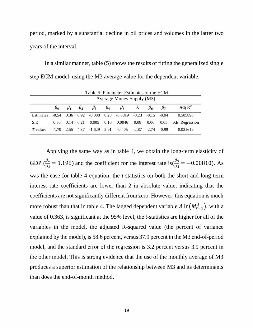
In a similar manner, table (5) shows the results of fitting the generalized single

step ECM model, using the M3 average value for the dependent variable.

Table 5: Parameter Estimates of the ECM

Average Money Supply (M3)

𝛽0 𝛽1 𝛽2 𝛽3 𝛽4 𝛽5 λ 𝛽6 𝛽7 Adj R2

Estimates -0.54 0.36 0.92 -0.008 0.28 -0.0019 -0.23 -0.15 -0.04 0.585896

S.E 0.30 0.14 0.21 0.005 0.10 0.0046 0.08 0.06 0.05 S.E. Regression

T-values -1.79 2.55 4.37 -1.629 2.91 -0.405 -2.87 -2.74 -0.99 0.031619

Applying the same way as in table 4, we obtain the long-term elasticity of

GDP (𝛽4

׀λ׀= 1.198) and the coefficient for the interest rate is(

𝛽5

׀λ׀= −0.00810). As

was the case for table 4 equation, the t-statistics on both the short and long-term

interest rate coefficients are lower than 2 in absolute value, indicating that the

coefficients are not significantly different from zero. However, this equation is much

more robust than that in table 4. The lagged dependent variable 𝛥 ln(𝑀𝑡−1𝑑 ), with a

value of 0.363, is significant at the 95% level, the t-statistics are higher for all of the

variables in the model, the adjusted R-squared value (the percent of variance

explained by the model), is 58.6 percent, versus 37.9 percent in the M3 end-of-period

model, and the standard error of the regression is 3.2 percent versus 3.9 percent in

the other model. This is strong evidence that the use of the monthly average of M3

produces a superior estimation of the relationship between M3 and its determinants

than does the end-of-month method.

20

6. Conclusion

The main objective of this paper is not to conduct a classic study of the

demand for money in Saudi Arabia. As it can be seen from the literature review, this

issue has been extensively studied. Rather, we aimed at exploring two questions that

are interrelated and data-driven. The first question is related to the historical monthly

and annual Hijra data that are present in many of the series published in previous

annual reports by SAMA. There can be no question on this issue since these data are

not accurate representations of the actual activities on the Gregorian dates that are

assumed to be correct by their users. Any attempt to use these historical data in

sophisticated econometric models that use time-dependent tools (e.g., autoregressive

lagged dependent variables, vector autoregression, error correction modeling, etc.,)

suffer from spurious estimations. Even a simple compound annual growth rate

calculation can be misleading, given the 354-355 day length of the Hijra year. The

conversion methodology used for the M3 data in this paper is only an approximation

of what the data would have actually been using a Gregorian calendar, but, in our

opinion, it is a far better way of handling the problem than continuing to use the

Hijra data as published.

The second question we addressed is the seeming mismatch of the statistical

data typically used in the simple money demand equations. This, in turn, suggests

the need for the used data to be consistent with no mismatch to ensure the accuracy

21

of the estimated results. Thus, the use of end-of-period data for items such as the

money supply, bank lending, and other financial balance sheet items, and attempting

to relate these data to variables that are expressed as averages or sums (e.g., income,

price levels, and interest rates) would seem to be inconsistent. It also causes serious

problems when combined with the Hijra data problem mentioned above.

The results of our analysis strongly suggest that the converted Hijra data are

capable of giving robust results when used in typical econometric analyses, with no

signs of instability in the short or long runs. In addition, they suggest that the use of

monthly average data for the money stock improves the stability and goodness-of-

fit of both the short and long-run ECM specifications. We are not

recommending that statistical agencies using Hijra calendar stop publishing their

data in the traditional format, but consideration should be given to using these

revised statistics in future research in this area.

22

Reference

Abdulkheir, A. Y. (2013). An Analytical Study of the Demand for Money in Saudi

Arabia. International Journal of Economics and Finance, 5 (4), 31 – 38.

Alkaswani, M., & Al-Towaijari, H. (1999). Cointegration, Error Correction and the

Demand for Money in Saudi Arabia. Economia Internazionale/ International

Economics, 52 (3), 299-308.

Al Rasasi, M. (2016). On the stability of money demand in Saudi Arabia. SAMA

Working Paper, No. 6/2016.

Al Rasasi, M., & Banafea, W. (2018). Estimating money demand function in Saudi

Arabia: evidence from cash in advance model. SAMA Working Paper, No.

4/2018.

Bahmani, S. (2008). “Stability of the Demand for Money in the Middle East.”

Emerging Markets Finance & Trade, 44 (1), 62 – 83.

Banafea, W. A. (2012). “Essays on structural breaks and stability of the money

demand function.” PhD Thesis, Kansas State University.

Banafea, W. A. (2014). “Endogenous Structural Breaks and Stability of the Money

Demand Function in Saudi Arabia.” International Journal of Economics and

Finance, 6 (1), 155 – 164.

Banerjee, A., Dolado, J.J., Galbraith, J.W., Hendry, D. (1993). Co-integration, error

correction, and the econometric analysis of non-stationary data. Oxford:

Oxford University Press.

De Boef, S. (2001). Modeling equilibrium relationship: error correction models with

strongly autoregressive data. Political Analysis, 9 (1), 78-94.

Dickey, D., & Fuller, W. (1979). Distribution of the estimators for autoregressive

time series with a unit root. Journal of the American Statistical Association,

74 (366), 427–431.

Elliot, G., Rothenberg, T.J., & Stock, J.H. (1996). Efficient tests for an

autoregressive unit root. Econometrica, 64 (4), 813-836.

23

Engle, R.F., & Granger, C.W.J. (1987). Co-integration and error correction:

Representation, estimation, and testing. Econometrica, 55 (2), 251-276.

Hamdi, H., Said, A., & Sbia, R. (2015). Empirical evidence on the long-run money

demand function in the Gulf Cooperation Council countries. International

Journal of Economics and Financial Issues, 5 (2), 603 – 612.

Harb, N. (2004). “Money demand function: a heterogeneous panel application.”

Applied Economics Letters, 11 (9), 551 – 555.

Hassanov, F. J., AL Rasasi, M. H., Al Sayaary, S., & Al-Fawzan, Z. (2017). Demand

for broad money in Saudi Arabian economy. SAMA Working Paper, No.

6/2017.

Johansen, S., & Juselius, K. (1990). Maximum likelihood estimated and inference

on cointegration with application to the demand for money. Oxford Bulletin

of Economics and Statistics, 52 (2), 169-210.

Kwiatkowski, D., Phillips, P.C.B., Schmidt, P., & Shin, Y. (1992). Testing the null

hypothesis of stationarity against the alternative of a unit root. Journal of

Econometrics, 54 (1-3), 159-178.

Lee, C., Chang, C., & Chen, P. (2008). “Money demand function versus monetary

integration: Revisiting panel cointegration among GCC countries.”

Mathematics and Computers in Simulation, 79(1), 85-93.

Phillips, P.C.B., & Perron, P. (1988). Testing for unit roots in time series regression.

Biometrika, 75 (2), 335-346.

Qualls, J.H., Algahtani, G. J., & Al Sayaary, S. (2017). Note on the Conversion of

annual and monthly data from the Hijra to the Gregorian calendar. SAMA

Working Paper, No. 17/7.