Embed Size (px)
Citation preview

Sahalu Junaidu ICS 573: High Performance Computing MPI.1
MPI Tutorial
• Examples Based on Michael Quinn’s Textbook
• Example 1: Circuit Satisfiability Check (Chapter 4)
• Example 2: Sieve of Eratosthenes (Chapter 5)
• Example 3: Floyd’s Algorithm (Chapter 6)
• Example 4: Matrix-Vector Multiplication (Chapter 8)
• Example 5: Document Classification (Chapter 9)

Sahalu Junaidu ICS 573: High Performance Computing MPI.2
Example 1: Circuit Satisfiability • This problem requires determining whether a given circuit is satisfiable.
– Find the set of input combinations (if any) for which the circuit output 1
• This problem is important for the design and verification of logical devices.
• This problem is NP-complete and one way to solve it is to try every combination of circuit inputs
• For a circuit with k inputs, there are 2k combinations since every input can take two values, 0 and 1.
• MPI functions introduced in this example– MPI_Init – to initialize MPI– MPI_Comm_rank – to determine a process’s ID number– MPI_Comm_size – to find the number of processes– MPI_Reduce – to perform a reduction operation– MPI_Finalize – to shut down MPI– MPI_Barrier – to perform barrier synchronization– MPI_Wtime – to determine the time– MPI_Wtick – to find the accuracy of the timer

Sahalu Junaidu ICS 573: High Performance Computing MPI.3
Example: Circuit Satisfiability
Sahalu Junaidu ICS 573: High Performance Computing MPI.4
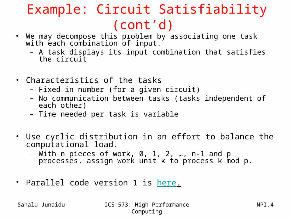
Example: Circuit Satisfiability (cont’d) • We may decompose this problem by associating one task with each
combination of input.– A task displays its input combination that satisfies the circuit
• Characteristics of the tasks– Fixed in number (for a given circuit)– No communication between tasks (tasks independent of each other)– Time needed per task is variable
• Use cyclic distribution in an effort to balance the computational load.– With n pieces of work, 0, 1, 2, …, n-1 and p processes, assign
work unit k to process k mod p.
• Parallel code version 1 is here.

Sahalu Junaidu ICS 573: High Performance Computing MPI.5
Example: Circuit Satisfiability (cont’d)
• Compiling: mpicc -o <exec> <source1> <source2> …
• Specifying host processors
• Running: mpirun -np <p> <exec> <arg1> …– -np <p> number of processes– <exec> executable– <arg1> … command-line arguments

Sahalu Junaidu ICS 573: High Performance Computing MPI.6
Example: Enhancing the Program
• We want to find total number of solutions
• Incorporate sum-reduction into program
• Modify function check_circuit– Return 1 if circuit satisfiable with input combination
– Return 0 otherwise
• Each process keeps local count of satisfiable circuits it has found
• Perform reduction after for loop
• This version of the program is here.

Sahalu Junaidu ICS 573: High Performance Computing MPI.7
Example: Benchmarking the Program • MPI_Barrier barrier synchronization• MPI_Wtime current time
– Returns an elapsed (wall clock) time on the calling processor • MPI_Wtick
– returns, as a double precision value, the number of seconds between successive clock ticks.
– For example, if the clock is implemented by the hardware as a counter that is incremented every millisecond, the value returned by MPI_WTICK should be 10-3
• Benchmarking code:
double elapsed_time;…
MPI_Init (&argc, &argv);MPI_Barrier (MPI_COMM_WORLD);elapsed_time = - MPI_Wtime();
…MPI_Reduce (…);elapsed_time += MPI_Wtime();

Sahalu Junaidu ICS 573: High Performance Computing MPI.8
Example: Benchmarking Result
Processors
Time (msec)
1 15.93
2 8.38
3 5.86
4 4.60
5 3.77
0
5
10
15
20
1 2 3 4 5
Processors
Tim
e (
ms
ec
)Execution Time
Perfect SpeedImprovement

Sahalu Junaidu ICS 573: High Performance Computing MPI.9
Profiling the Circuit Satisfiability Program

Sahalu Junaidu ICS 573: High Performance Computing MPI.10
Profiling the Circuit Satisfiability Program

Sahalu Junaidu ICS 573: High Performance Computing MPI.11
Profiling the Circuit Satisfiability Program

Sahalu Junaidu ICS 573: High Performance Computing MPI.12
Discussion • Assume n pieces of work, p processes, and cyclic
allocation– What is the most pieces of work any process has?– What is the least pieces of work any process has?– How many processes have the most pieces of work?

Sahalu Junaidu ICS 573: High Performance Computing MPI.13
Example 2: Sieve of Eratosthenes
• Sieve of Eratosthenes is a classical way of extracting prime numbers from a series of all integers starting from 2
• First number, 2, is prime and kept.
• All multiples of this number are deleted as they cannot be prime.
• Process repeated with each remaining number.
• The algorithm removes nonprimes, leaving only primes.
• MPI function introduced in this example– MPI_Bcast – to broadcast a message to all processes in a communicator

Sahalu Junaidu ICS 573: High Performance Computing MPI.14
Sieve of Eratosthenes: Sequential Algorithm
2 3 4 5 6 7 8 9 10 11 12 13 14 15 16
17 18 19 20 21 22 23 24 25 26 27 28 29 30 31
32 33 34 35 36 37 38 39 40 41 42 43 44 45 46
47 48 49 50 51 52 53 54 55 56 57 58 59 60 61
2 4 6 8 10 12 14 16
18 20 22 24 26 28 30
32 34 36 38 40 42 44 46
48 50 52 54 56 58 60
3 9 15
21 27
33 39 45
51 57
5
25
35
55
7
49

Sahalu Junaidu ICS 573: High Performance Computing MPI.15
Sieve of Eratosthenes: Sequential Algorithm
for(i=2; i<=n; i++)
prime[i] = 0; /* initialize array */
for(i=2; i<=sqrt_n; i++) /* for each prime */
if (prime[i]==0)
for(j=i*i; j<=n; j = j+i)
prime[j] = 1; /* strike its multiples */

Sahalu Junaidu ICS 573: High Performance Computing MPI.16
Sieve of Eratosthenes: Sequential Algorithm
1. Create list of unmarked natural numbers 2, 3, …, n2. k 23. Repeat
(a) Mark all multiples of k between k2 and n(b) k smallest unmarked number > k
until k2 > n4. The unmarked numbers are primes

Sahalu Junaidu ICS 573: High Performance Computing MPI.17
Making 3(a) Parallel
Mark all multiples of k between k2 and n
for all j where k2 j n do if j mod k = 0 then mark j (it is not a prime) endifendfor

Sahalu Junaidu ICS 573: High Performance Computing MPI.18
Making 3(b) Parallel
• Find smallest unmarked number > k
• Min-reduction (to find smallest unmarked number > k)
• Broadcast (to get result to all tasks)

Sahalu Junaidu ICS 573: High Performance Computing MPI.19
Sieve of Eratosthenes: Parallelization Options
• Make each process handle one array element– Lots of data parallelism– Lots of communication (a reduce and a broadcast in each
iteration)
• Make each process strike out one number– Leads to load imbalance– Repeated work when done naively
• Pipelining
• Cyclic allocation– Leads to load imbalance for this problem – Easy to determine “owner” of each index
• Block allocation– Balances loads– More complicated to determine owner if n not a multiple of p

Sahalu Junaidu ICS 573: High Performance Computing MPI.20
Advantages of Block Decomposition: No Reduction
• Largest prime used to sieve is n
• First process has n/p elements
• It has all sieving primes if p < n
• First process always broadcasts next sieving prime
• No reduction step needed

Sahalu Junaidu ICS 573: High Performance Computing MPI.21
Advantages of Block Decomposition: Fast Marking
• Block decomposition allows same marking as sequential algorithm:
j, j + k, j + 2k, j + 3k, …
instead of
for all j in blockif j mod k = 0 then mark j (it is not a prime)

Sahalu Junaidu ICS 573: High Performance Computing MPI.22
Block Decomposition Macros
#define BLOCK_LOW(id,p,n) ((i)*(n)/(p))
#define BLOCK_HIGH(id,p,n) \ (BLOCK_LOW((id)+1,p,n)-1)
#define BLOCK_SIZE(id,p,n) \ (BLOCK_HIGH(id,p,n)-BLOCK_LOW(id,p,n)+1)
#define BLOCK_OWNER(index,p,n) \ (((p)*(index)+1)-1)/(n))

Sahalu Junaidu ICS 573: High Performance Computing MPI.23
Function MPI_Bcast
int MPI_Bcast (
void *buffer, /* Addr of 1st element */
int count, /* # elements to broadcast */
MPI_Datatype datatype, /* Type of elements */
int root, /* ID of root process */
MPI_Comm comm) /* Communicator */
MPI_Bcast (&k, 1, MPI_INT, 0, MPI_COMM_WORLD);
• Complete code is here.

Sahalu Junaidu ICS 573: High Performance Computing MPI.24
Benchmarking the Sieve ProgramProcessor Times (sec) Relative Speedup
1 12.49 12 6.79 1.843 5.1 2.454 4.17 35 3.88 3.226 3.44 3.637 3.15 3.978 2.73 4.589 2.62 4.77
10 4.83 2.59
Sieve Primes from 2 to 100 Million Numbers (160 Runs)
0
2
4
6
8
10
12
14
0 1 2 3 4 5 6 7 8 9
Processors
Tim
e (s
ec)

Sahalu Junaidu ICS 573: High Performance Computing MPI.25
Profiling the Sieve Program

Sahalu Junaidu ICS 573: High Performance Computing MPI.26
Profiling the Sieve Program
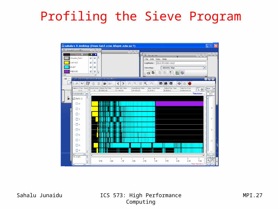
Sahalu Junaidu ICS 573: High Performance Computing MPI.27
Profiling the Sieve Program

Sahalu Junaidu ICS 573: High Performance Computing MPI.28
Improving the Sieve Program
• The performance of the Sieve program can be improved by– Deleting even integers– Eliminating broadcast
• If only odd integers are represented – storage requirements of the program can be halved and – the speed of marking multiples of a particular prime can be
doubled• Eliminate broadcast by replicating the odd integers 3, 5, 7, …, n on each process– Each process can then use the sequential algorithm to find the
primes in this range– After that each process can sieve its n/p portion of the larger
array without a broadcast

Sahalu Junaidu ICS 573: High Performance Computing MPI.29
Results After Removing Even IntegersProcessor Time (sec) Relative Speedup
1 6.38 12 3.9 1.643 3.12 2.044 2.7 2.365 2.49 2.566 2.48 2.577 2.33 2.748 2.3 2.77
Sieve from 2 to 100 Million (without Even Numbers) (160 Runs)
0
1
2
3
4
5
6
7
0 1 2 3 4 5 6 7 8 9
Processors
Tim
es (
sec)

Sahalu Junaidu ICS 573: High Performance Computing MPI.30
Jumpshot Visualization After Removing Even Integers

Sahalu Junaidu ICS 573: High Performance Computing MPI.31
Jumpshot Visualization After Removing Even Integers
Sahalu Junaidu ICS 573: High Performance Computing MPI.32
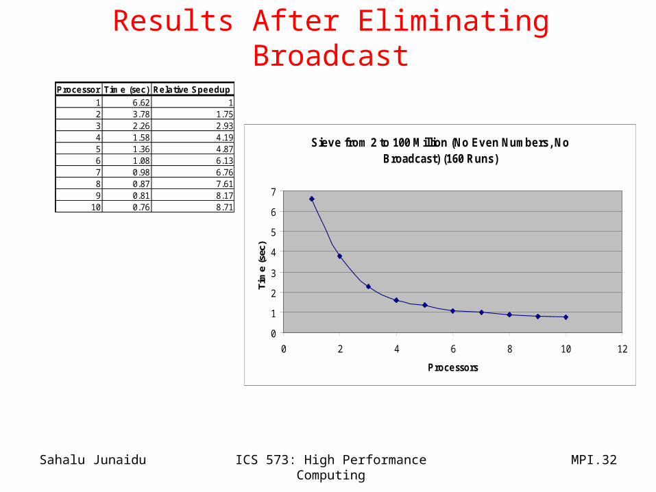
Results After Eliminating Broadcast
Processor Time (sec) Relative Speedup
1 6.62 12 3.78 1.753 2.26 2.934 1.58 4.195 1.36 4.876 1.08 6.137 0.98 6.768 0.87 7.619 0.81 8.17
10 0.76 8.71
Sieve from 2 to 100 Million (No Even Numbers, No Broadcast) (160 Runs)
0
1
2
3
4
5
6
7
0 2 4 6 8 10 12
Processors
Tim
e (s
ec)

Sahalu Junaidu ICS 573: High Performance Computing MPI.33
Results SummaryProcessor Original No evens No broadcast
1 12.49 6.38 6.622 6.79 3.9 3.783 5.1 3.12 2.264 4.17 2.7 1.585 3.88 2.49 1.366 3.44 2.48 1.087 3.15 2.33 0.988 2.73 2.3 0.87
Runtimes (sec)
Sieve from 2 to 100 Million Numbers (160 Runs in each case)
0
2
4
6
8
10
12
14
0 2 4 6 8 10
Processors
Tim
es (
sec) Original
No evens
No broadcast

Sahalu Junaidu ICS 573: High Performance Computing MPI.34
Jumpshot Visualization After Eliminating Broadcast

Sahalu Junaidu ICS 573: High Performance Computing MPI.35
Example 3: Floyd’s Algorithm • Floyd’s algorithm is a classic algorithm used to solve the all-pairs
shortest-path problem.
• It uses the dynamic programming (DP) method to solve the problem on a dense graph.
• DP is used to solve a wide variety of discrete optimization problems such as scheduling, etc.
• DP breaks problems into subproblems and combine their solutions into solutions to larger problems.
• In contrast to divide-and-conquer, there may be interrelationships across subproblems.
• MPI functions introduced in this example– MPI_Send – which allows a process to send a message to another process– MPI_Recv – which allows a process to receive a message from another process

Sahalu Junaidu ICS 573: High Performance Computing MPI.36
Sequential Floyd’s Algorithm
for k 0 to n-1for i 0 to n-1
for j 0 to n-1a[i,j] min (a[i,j], a[i,k] + a[k,j])
endfor
endfor
endfor

Sahalu Junaidu ICS 573: High Performance Computing MPI.37
Executing Floyd’s Algorithm
A
E
B
C
D
4
6
1 35
3
1
2
0 6 3 6
4 0 7 10
12 6 0 3
7 3 10 0
9 5 12 2
A
B
C
D
E
A B C D
4
8
1
11
0
E
Resulting Adjacency Matrix Containing Distances

Sahalu Junaidu ICS 573: High Performance Computing MPI.38
Tracing Floyd’s Algorithm (iteration k=0)
i=0,j=0,1,2,3,4A[0,0]=MIN(A[0,0],A[0,0]+A[0,0])=0A[0,1]=MIN(A[0,1],A[0,0]+A[0,1])=6A[0,2]=MIN(A[0,2],A[0,0]+A[0,2])=3A[0,3]=MIN(A[0,3],A[0,0]+A[0,3])=INFA[0,4]=MIN(A[0,4],A[0,0]+A[0,4])=INF
i=3,j=0,1,2,3,4A[3,0]=MIN(A[3,0],A[3,0]+A[0,0])=INFA[3,1]=MIN(A[3,1],A[3,0]+A[0,1])=3A[3,2]=MIN(A[3,2],A[3,0]+A[0,2])=INFA[3,3]=MIN(A[3,3],A[3,0]+A[0,3])=0A[3,4]=MIN(A[3,4],A[3,0]+A[0,4])=INF
i=1,j=0,1,2,3,4A[1,0]=MIN(A[1,0],A[1,0]+A[0,0])=4A[1,1]=MIN(A[1,1],A[1,0]+A[0,1])=0A[1,2]=MIN(A[1,2],A[1,0]+A[0,2])=7A[1,3]=MIN(A[1,3],A[1,0]+A[0,3])=1A[1,4]=MIN(A[1,4],A[1,0]+A[0,4])=INF
i=4,j=0,1,2,3,4A[4,0]=MIN(A[4,0],A[4,0]+A[0,0])=INFA[4,1]=MIN(A[4,1],A[4,0]+A[0,1])=INFA[4,2]=MIN(A[4,2],A[4,0]+A[0,2])=INFA[4,3]=MIN(A[4,3],A[4,0]+A[0,3])=2A[4,4]=MIN(A[4,4],A[4,0]+A[0,4])=0
i=2,j=0,1,2,3,4A[2,0]=MIN(A[2,0],A[2,0]+A[0,0])=INFA[2,1]=MIN(A[2,1],A[2,0]+A[0,1])=INFA[2,2]=MIN(A[2,2],A[2,0]+A[0,2])=0A[2,3]=MIN(A[2,3],A[2,0]+A[0,3])=5A[2,4]=MIN(A[2,4],A[2,0]+A[0,4])=1
02
03
150
1704
360
)1(D

Sahalu Junaidu ICS 573: High Performance Computing MPI.39
Tracing Floyd’s Algorithm (iteration k = 1)
i=0,j=0,1,2,3,4A[0,0]=MIN(A[0,0],A[0,1]+A[1,0])=0A[0,1]=MIN(A[0,1],A[0,1]+A[1,1])=6A[0,2]=MIN(A[0,2],A[0,1]+A[1,2])=3A[0,3]=MIN(A[0,3],A[0,1]+A[1,3])=7A[0,4]=MIN(A[0,4],A[0,1]+A[1,4])=INF
i=3,j=0,1,2,3,4A[3,0]=MIN(A[3,0],A[3,1]+A[1,0])=7A[3,1]=MIN(A[3,1],A[3,1]+A[1,1])=3A[3,2]=MIN(A[3,2],A[3,1]+A[1,2])=10A[3,3]=MIN(A[3,3],A[3,1]+A[1,3])=0A[3,4]=MIN(A[3,4],A[3,1]+A[1,4])=INF
i=1,j=0,1,2,3,4A[1,0]=MIN(A[1,0],A[1,1]+A[1,0])=4A[1,1]=MIN(A[1,1],A[1,1]+A[1,1])=0A[1,2]=MIN(A[1,2],A[1,1]+A[1,2])=7A[1,3]=MIN(A[1,3],A[1,1]+A[1,3])=1A[1,4]=MIN(A[1,4],A[1,1]+A[1,4])=INF
i=4,j=0,1,2,3,4A[4,0]=MIN(A[4,0],A[4,1]+A[1,0])=INFA[4,1]=MIN(A[4,1],A[4,1]+A[1,1])=INFA[4,2]=MIN(A[4,2],A[4,1]+A[1,2])=INFA[4,3]=MIN(A[4,3],A[4,1]+A[1,3])=2A[4,4]=MIN(A[4,4],A[4,1]+A[1,4])=0
i=2,j=0,1,2,3,4A[2,0]=MIN(A[2,0],A[2,1]+A[1,0])=INFA[2,1]=MIN(A[2,1],A[2,1]+A[1,1])=INFA[2,2]=MIN(A[2,2],A[2,1]+A[1,2])=0A[2,3]=MIN(A[2,3],A[2,1]+A[1,3])=5A[2,4]=MIN(A[2,4],A[2,1]+A[1,4])=1
02
01037
150
1704
7360
)2(D

Sahalu Junaidu ICS 573: High Performance Computing MPI.40
Designing Parallel Algorithm
• From the pseudocode, we see that the same assignment statement is executed n3 times– Decompose the problem by dividing matrix A into its n2 elements
• Communication– Each update of element a[i,j] requires access to elements a[i,k] and a[k,j]
– Note that for any particular k, element a[k,m] is needed by every task associated with elements in column m.
• Thus, during iteration k each element in row k of gets broadcast to the tasks in the same column
– Similarly, for any particular value of k, element a[m,k] is needed by every task associated with elements in row m.
• Thus, during iteration k each element in column k of a gets broadcast to the tasks in the same row

Sahalu Junaidu ICS 573: High Performance Computing MPI.41
Floyd’s Algorithm: Partitioning and Communication
Primitive tasksUpdatinga[3,4] whenk = 1
Iteration k:every taskin row kbroadcastsits value w/intask column
Iteration k:every taskin column kbroadcastsits value w/intask row

Sahalu Junaidu ICS 573: High Performance Computing MPI.42
Designing Parallel Algorithm
• Can the elements of the distance matrix be updated simultaneously?
• That is, must a[i,k] and a[k,j] be computed before updating a[i,j] ?
• The answer is no since the values a[i,k] and a[k,j] do not change during iteration k.
• That is, during iteration k, updates to a[i,k] and a[k,j] take the forms:– a[i,k] min (a[i,k], a[i,k] + a[k,k])– a[k,j] min (a[k,j], a[k,k] + a[k,j])
• Since all values are positive, neither a[i,k] nor a[k,j]can decrease.
• Thus for each iteration k of the outer loop, we can perform the broadcasts and then update every element of the matrix in parallel.

Sahalu Junaidu ICS 573: High Performance Computing MPI.43
Designing Parallel Algorithm
• Tasks characteristics:– Number of tasks: static– Communication pattern among tasks: structured– Computation time per task: constant– Strategy:
• Agglomerate tasks to minimize communication, creating one task per MPI process
• That is, agglomerate n2 primitive tasks into p processes
• Columnwise block striped– Broadcast within columns eliminated
• Rowwise block striped– Broadcast within rows eliminated– Reading matrix from file simpler
• Choose rowwise block striped decomposition

Sahalu Junaidu ICS 573: High Performance Computing MPI.44
Matrix I/O Functions
void read_row_striped_matrix ( char *s, /* IN - File name */ void ***subs, /* OUT - 2D submatrix indices */ void **storage, /* OUT - Submatrix stored here */ MPI_Datatype dtype, /* IN - Matrix element type */ int *m, /* OUT - Matrix rows */ int *n, /* OUT - Matrix cols */ MPI_Comm comm) /* IN - Communicator */
void print_row_striped_matrix ( void **a, /* IN - 2D array */ MPI_Datatype dtype, /* IN - Matrix element type */ int m, /* IN - Matrix rows */ int n, /* IN - Matrix cols */ MPI_Comm comm) /* IN - Communicator */
• The complete parallel program is here.

Sahalu Junaidu ICS 573: High Performance Computing MPI.45
Benchmarking the Floyd’s Program
Processor Time (sec) Relative Speedup
1 13.43 12 7.04 1.913 4.79 2.84 3.69 3.645 3.02 4.456 2.62 5.137 2.23 6.028 1.95 6.899 1.81 7.42
10 1.63 8.2411 1.48 9.0712 1.42 9.46
Floyd's Algorithm on a 1,000 by 1,000 Dense Matrix (20 runs)
0
2
4
6
8
10
12
14
16
0 2 4 6 8 10 12 14
Processors
Tim
e (
se
c)

Sahalu Junaidu ICS 573: High Performance Computing MPI.46
Profiling the Floyd’s Program

Sahalu Junaidu ICS 573: High Performance Computing MPI.47
Example 4: Matrix-Vector Multiplication • Matrix-vector multiplication is embedded in algorithms solving a wide variety of
problems, like:– Iterative algorithms for solving systems of linear equations– Implementation of neural networks
• In this example, we develop three MPI programs to multiply a dense matrix by a vector, each based on a different data decomposition
• MPI functions introduced in this example– MPI_Allgatherv – an all-gather function in which different processes may contribute
different numbers of elements– MPI_Scatterv – a scatter operation in which different processes may end up with different
numbers of elements– MPI_Gatherv – a gather operation in which the number of elements collected from different
process may vary– MPI_Alltoall – an all-to-all exchange of data elements among processes– MPI_Dims_create – provides dimensions for a balanced Cartesian grid of processes– MPI_Cart_create – creates a communicator where the processes have a Cartesian
topology– MPI_Cart_coords – returns the coordinates of a specified process within a Cartesian grid– MPI_Cart_rank – returns the rank of the process at specified coordinates in a Cartesian
grid– MPI_Comm_split – partitions the processes of an existing communicator into one or more
groups

Sahalu Junaidu ICS 573: High Performance Computing MPI.48
Matrix-Vector Multiplication: Sequential Algorithm
Input: a[0..m-1,0..n-1] – an m x n matrix b[0..n-1] – an n x 1 vector
Output: c[0..m-1] – an m x 1 vector
for i 0 to m-1 c[i] 0 for j 0 to n-1
c[i] c[i]+ a[i,j] * b[j] endfor
endfor
• Matrix-vector multiplication is simply a series of inner product (dot product) computations

Sahalu Junaidu ICS 573: High Performance Computing MPI.49
Data Decomposition Options
• Three decomposition options for an m x n matrix:– Rowwise block-striped
• Each process responsible for a contiguous group of or rows of the matrix
– Columnwise block-striped• Each process responsible for a contiguous group of or columns of the
matrix
– Checkerboard block• Processes form a virtual grid, and the matrix is divided into 2-D blocks
aligning with that grid• Given a p-processor grid with r rows and c columns, each process is
responsible for a block of the matrix containing at most rows and columns
• Vectors distribution options– Replicated both vectors on each process– Block distribution option: each of the p processes is responsible for a
contiguous group of either or vector elements
p
n
p
n
p
n
p
n
p
m
p
m
r
m
c
n

Sahalu Junaidu ICS 573: High Performance Computing MPI.50
Example 4.1: Rowwise Block-Striped Decomposition
• This version of the program is based on – Rowwise block-striped decompositions– Replicated vectors
• First, we associate a primitive task with – each row of the matrix– replicated argument and result vectors
• Tasks characteristics– Static number of tasks– Regular communication pattern (all-gather)– Computation time per task is constant– Strategy: Agglomerate groups of rows, creating one task per MPI
process
• When tasks are combined in this way, each process will compute a block of elements of the result vector.– These need to be combined to ensure that each process has all
elements of the result vector
Sahalu Junaidu ICS 573: High Performance Computing MPI.51
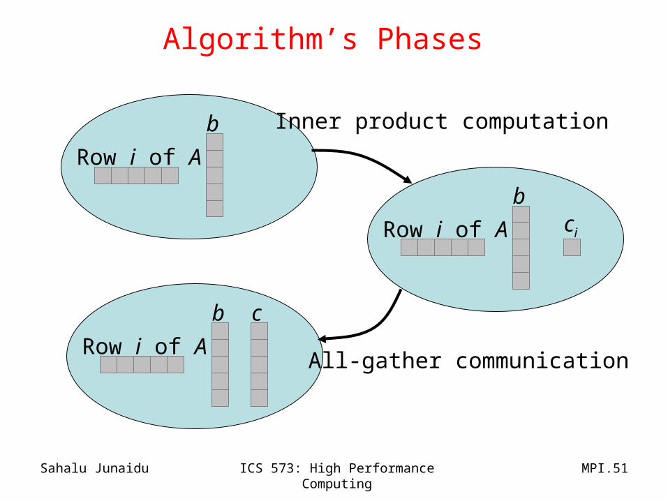
Algorithm’s Phases
Row i of A
b
Row i of A
bci
Inner product computation
Row i of A
b c
All-gather communication

Sahalu Junaidu ICS 573: High Performance Computing MPI.52
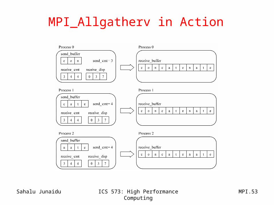
Replicating a Block-Mapped Vector
• The block of elements of the result vector computed by each process can be replicated using MPI_Allgatherv:– If the same number of items is gathered from every process, the simpler
MPI_Allgather is appropriate.
int MPI_Allgatherv ( void *send_buffer, int send_cnt, MPI_Datatype send_type, void *receive_buffer, int *receive_cnt, int *receive_disp, MPI_Datatype receive_type, MPI_Comm communicator)
Sahalu Junaidu ICS 573: High Performance Computing MPI.53
MPI_Allgatherv in Action
Sahalu Junaidu ICS 573: High Performance Computing MPI.54
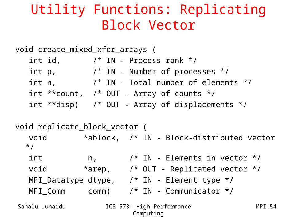
Utility Functions: Replicating Block Vector
void create_mixed_xfer_arrays (
int id, /* IN - Process rank */
int p, /* IN - Number of processes */
int n, /* IN - Total number of elements */
int **count, /* OUT - Array of counts */
int **disp) /* OUT - Array of displacements */
void replicate_block_vector (
void *ablock, /* IN - Block-distributed vector */
int n, /* IN - Elements in vector */
void *arep, /* OUT - Replicated vector */
MPI_Datatype dtype, /* IN - Element type */
MPI_Comm comm) /* IN - Communicator */

Sahalu Junaidu ICS 573: High Performance Computing MPI.55
Utility Functions: Matrix & Vector Inputvoid read_row_striped_matrix ( char *s, /* IN - File name */ void ***subs, /* OUT - 2D submatrix indices */ void **storage, /* OUT - Submatrix stored here */ MPI_Datatype dtype, /* IN - Matrix element type */ int *m, /* OUT - Matrix rows */ int *n, /* OUT - Matrix cols */ MPI_Comm comm) /* IN - Communicator */
void read_replicated_vector ( char *s, /* IN - File name */ void **v, /* OUT - Vector */ MPI_Datatype dtype, /* IN - Vector type */ int *n, /* OUT - Vector length */ MPI_Comm comm) /* IN - Communicator */
• The complete parallel program is here.
Sahalu Junaidu ICS 573: High Performance Computing MPI.56
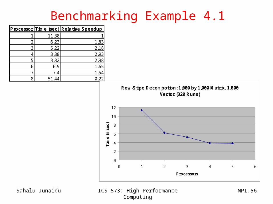
Benchmarking Example 4.1Processor Time (sec) Relative Speedup
1 11.38 12 6.23 1.833 5.22 2.184 3.88 2.935 3.82 2.986 6.9 1.657 7.4 1.548 51.44 0.22
Row-Stipe Decompotion: 1,000 by 1,000 Matrix, 1,000 Vector (320 Runs)
0
2
4
6
8
10
12
0 1 2 3 4 5 6
Processors
Tim
e (m
sec)

Sahalu Junaidu ICS 573: High Performance Computing MPI.57
Profiling Example 4.1

Sahalu Junaidu ICS 573: High Performance Computing MPI.58
Profiling Example 4.1

Sahalu Junaidu ICS 573: High Performance Computing MPI.59
Example 4.2: Columnwise Block-Striped Decomposition
• This version of the program is based on – Columnwise block-striped decompositions– Block-decomposed vectors
• First, we associate a primitive task i with – column i of the matrix– elements i of the argument and result vectors
• Tasks characteristics– Static number of tasks– Regular communication pattern (all-to-all exchange)– Computation time per task is constant– Strategy: Agglomerate the primitive tasks into metatasks, mapping a
metatask to an MPI process
• When tasks are combined in this way, each process will compute a block of elements of the result vector.– These need to be combined to ensure that each process has all
elements of the result vector

Sahalu Junaidu ICS 573: High Performance Computing MPI.60
Algorithm’s PhasesC
olum
n i o
f A
b
Col
umn
i of
A
b ~cMultiplications
Col
umn
i of
A
b ~c
All-to-all exchange
Col
umn
i of
A
b c
Reduction

Sahalu Junaidu ICS 573: High Performance Computing MPI.61
Exchanging Partial Inner Products
• Communication required for primitive task i to produce a single element of the result vector:– All-to-all communication: every partial result element j on task i
must be transferred to task j• i.e., each task distributes n-1 terms it does not need and collect n-1
terms that it needs– At this point every task i has the n partial results it needs to add
in order to produce c[i]
• The same principle is extended to each metatask– Each process exchanges blocks it does not need for blocks it
needs– Each metatask i receives BLOCK_SIZE(i,p,n) elements from
each other task– After the exchange, i has p subarrays of size BLOCK_SIZE(i,p,n) which it needs to add to form its block of the result vector.

Sahalu Junaidu ICS 573: High Performance Computing MPI.62
Function MPI_Alltoallv
int MPI_Alltoallv (
void *send_buffer,
int *send_cnt,
int *send_disp,
MPI_Datatype send_type,
void *receive_buffer,
int *receive_cnt,
int *receive_disp,
MPI_Datatype receive_type,
MPI_Comm communicator)
Sahalu Junaidu ICS 573: High Performance Computing MPI.63
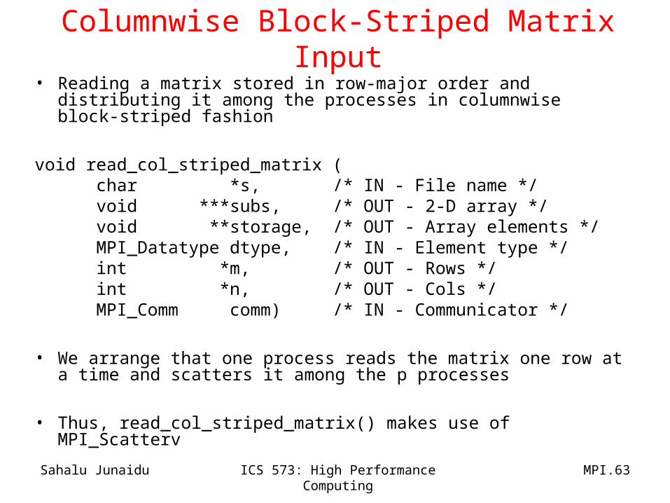
Columnwise Block-Striped Matrix Input• Reading a matrix stored in row-major order and distributing it among
the processes in columnwise block-striped fashion
void read_col_striped_matrix ( char *s, /* IN - File name */ void ***subs, /* OUT - 2-D array */ void **storage, /* OUT - Array elements */ MPI_Datatype dtype, /* IN - Element type */ int *m, /* OUT - Rows */ int *n, /* OUT - Cols */ MPI_Comm comm) /* IN - Communicator */
• We arrange that one process reads the matrix one row at a time and scatters it among the p processes
• Thus, read_col_striped_matrix() makes use of MPI_Scatterv

Sahalu Junaidu ICS 573: High Performance Computing MPI.64
Function MPI_Scatterv
int MPI_Scatterv (
void *send_buffer,
int *send_cnt,
int *send_disp,
MPI_Datatype send_type,
void *receive_buffer,
int receive_cnt,
MPI_Datatype receive_type,
int root,
MPI_Comm communicator)

Sahalu Junaidu ICS 573: High Performance Computing MPI.65
Columnwise Block-Striped Matrix Output
• To ensure that values of the result matrix are printed row-wise and in correct order:– Let a single process does the printing
– A gather operation is needed to print elements of each row (opposite dataflow to that of input)
void print_col_striped_matrix (
void **a, /* IN - 2D array */
MPI_Datatype dtype, /* IN - Type of matrix elements */
int m, /* IN - Matrix rows */
int n, /* IN - Matrix cols */
MPI_Comm comm) /* IN - Communicator */
• print_col_striped_matrix() makes use of MPI_Gatherv

Sahalu Junaidu ICS 573: High Performance Computing MPI.66
Function MPI_Gatherv
int MPI_Gatherv ( void *send_buffer, int send_cnt, MPI_Datatype send_type, void *receive_buffer, int *receive_cnt, int *receive_disp, MPI_Datatype receive_type, int root, MPI_Comm communicator)
• Example 4.2 parallel program is here.

Sahalu Junaidu ICS 573: High Performance Computing MPI.67
Benchmarking Example 4.2Processor Time (sec) Relative Speedup
1 18.93 12 5.88 3.223 4.33 4.374 4.12 4.595 4.07 4.656 6.73 2.817 6.73 2.818 178.82 0.11
Column-Striped Distribution: 1,000 by 1,000 Matrix, 1,000 Vector (320 Runs)
0
5
10
15
20
0 1 2 3 4 5 6
Processors
Tim
e (m
sec)

Sahalu Junaidu ICS 573: High Performance Computing MPI.68
Profiling Example 4.2

Sahalu Junaidu ICS 573: High Performance Computing MPI.69
Example 4.3: Checkerboard Block Decomposition
• This version of the program is based on – Checkerboard (2-D) block decomposition of the matrix– Block-decomposed vectors among processes in the first column of the process
grid
• First, we associate a primitive task i with – an element of the matrix
• Each primitive task performs one multiply
• Agglomerate primitive tasks into rectangular blocks
• Processes form a 2-D grid
• The argument vector is distributed by blocks among processes in first column of grid

Sahalu Junaidu ICS 573: High Performance Computing MPI.70
Algorithm’s Phases

Sahalu Junaidu ICS 573: High Performance Computing MPI.71
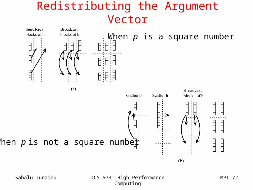
Redistributing the Argument Vector
• Task associated with matrix block Ai,j performs a matrix-vector multiplication of this block with subvector bj.
• Thus, we need to redistribute the vector so that each task has the correct portion of the vector
• Assume the p tasks are divided into a k x l grid
• Initially, divide the vector among the k tasks in the first column of the task grid– After the distribution, a copy of the vector is divided among the l tasks in each row
• Case 1: k=l– Task at grid position (i,0) send its portion of the vector to task at position (0,i)– Then, each process in the first row of the task grid broadcasts its portion of the vector to
tasks in its column
• Case 2: k /= l– First gather the elements of the vector onto the task at grid position (0,0)– Next, scatter the elements of the vector among the tasks in the first row of the grid– Finally, each process in the first row of the task grid broadcasts its portion of the vector to the
other tasks in the same column
Sahalu Junaidu ICS 573: High Performance Computing MPI.72
Redistributing the Argument Vector
When p is a square number
When p is not a square number

Sahalu Junaidu ICS 573: High Performance Computing MPI.73
Creating a Communicator• MPI_COMM_WORLD is the default communicator used when all
processes are involved in collective communication.
• When a subset of the processes are involved in communication, a new communicator has to be created.
• Communication instances in Example 4.3 involving subsets of processes– Gathering vector b among processes in the first column of the virtual
process grid (when p is not square).– Scattering vector b among processes in the first row of the virtual
process grid (when p is not square).– Broadcasting a block of b by each first-row process along its column.– Performing independent sum-reductions along each row to produce the
result vector.
• A communicator is a process group one of whose important attributes is topology.
– A communicator’s topology enables associating an addressing scheme with the processes, other than the rank.

Sahalu Junaidu ICS 573: High Performance Computing MPI.74
Creating a Virtual Process Grid
• Function MPI_Dims_create creates a virtual process grid that is as close to a square as possible.
int MPI_Dims_create ( int nodes, /* Input - Processes in grid */ int dims, /* Input - Number of dimensions */ int *size) /* Input/Output - Size of each grid
dimension */
• The elements of size must be initialized before calling the function– If size[i]=0, the function can determine that dimension,
otherwise it has been determined by the programmer.
Sahalu Junaidu ICS 573: High Performance Computing MPI.75
Creating a Virtual Process Grid
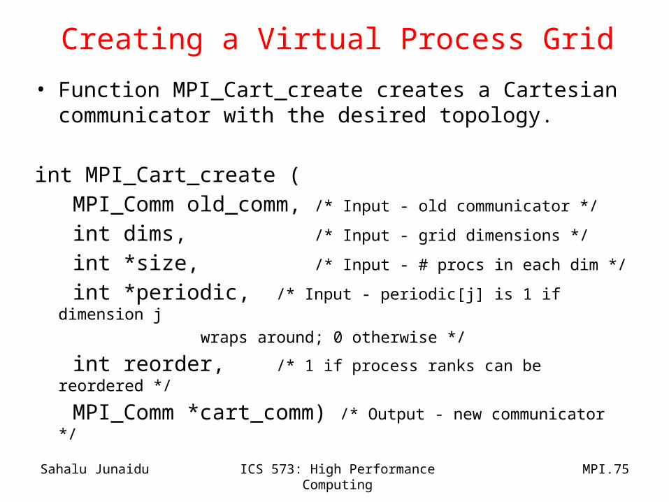
• Function MPI_Cart_create creates a Cartesian communicator with the desired topology.
int MPI_Cart_create ( MPI_Comm old_comm, /* Input - old communicator */
int dims, /* Input - grid dimensions */
int *size, /* Input - # procs in each dim */
int *periodic, /* Input - periodic[j] is 1 if dimension j
wraps around; 0 otherwise */
int reorder, /* 1 if process ranks can be reordered */
MPI_Comm *cart_comm) /* Output - new communicator */

Sahalu Junaidu ICS 573: High Performance Computing MPI.76
Cartesian Communicator for Example 4.3
MPI_Comm cart_comm;int p;int periodic[2];int size[2];...size[0] = size[1] = 0;MPI_Dims_create (p, 2, size);periodic[0] = periodic[1] = 0;MPI_Cart_create (MPI_COMM_WORLD, 2, size, 1, &cart_comm);
• Here is a complete example program.

Sahalu Junaidu ICS 573: High Performance Computing MPI.77
Checkberboard Matrix Input
• The distribution pattern in this case is similar to that in columnwise striping– Difference: a row is scattered among a subset of the processes in this
case (those in the same row of the virtual process grid)
• We assume, as before, that one process is responsible for input
• Each time the input process reads a row, it sends it to the first process in the appropriate row of the process grid– The first-row process then scatters the row among processes in its row
of the process grid
• The following grid-relation functions are needed to accomplish the matrix input:
int MPI_Cart_rank ()int MPI_Cart_coords ()int MPI_Comm_split ()
Sahalu Junaidu ICS 573: High Performance Computing MPI.78
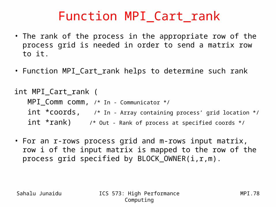
Function MPI_Cart_rank
• The rank of the process in the appropriate row of the process grid is needed in order to send a matrix row to it.
• Function MPI_Cart_rank helps to determine such rank
int MPI_Cart_rank ( MPI_Comm comm, /* In - Communicator */
int *coords, /* In - Array containing process’ grid location */
int *rank) /* Out - Rank of process at specified coords */
• For an r-rows process grid and m-rows input matrix, row i of the input matrix is mapped to the row of the process grid specified by BLOCK_OWNER(i,r,m).

Sahalu Junaidu ICS 573: High Performance Computing MPI.79
A Process’ Rank in A Virtual Process Grid
int dest_coord[2]; /* coordinates of process receiving row */int dest_id; /* rank of process receiving row */int grid_id; /* rank of process in virtual grid */int i;…for(i=0;i<m;i++){ dest_coord[0]=BLOCK_OWNER(i,r,m); dest_coord[1]=0; grid_id=MPI_Cart_rank(grid_comm,dest_coord,&dest_id); if(grid_id==0){ /* Read matrix row ‘i’ */ … /* Send matrix row ‘i’ to process ‘dest_id’ */ }else if (grid_id==dest_id){ /* Receive matrix row ‘i’ from process 0 */ … }}

Sahalu Junaidu ICS 573: High Performance Computing MPI.80
A Process’ Coordinates in A Virtual Process Grid
• Function MPI_Cart_coord determines the coordinates of a process in a virtual process grid
• Uses in Example 4.3:– Allows a process to allocate the correct amount of memory for its portion
of the matrix and the vector– Enables process 0 to avoid sending itself a message if it happens to be
the first in a row of the process grid
int MPI_Cart_coords ( MPI_Comm comm, /* In - Communicator */
int rank, /* In - Rank of process */
int dims, /* In - Dimensions in virtual grid */
int *coords) /* Out - Coordinates of specified process in virtual grid */

Sahalu Junaidu ICS 573: High Performance Computing MPI.81
Splitting a Cartesian Communicator into Groups
• The Cartesian communicator needs to be split into groups for every row in the process grid– Needed for columnwise scatter and rowwise reduce
• Function MPI_Comm_split is used to achieve this
int MPI_Comm_split ( MPI_Comm old_comm, /* In - Existing communicator */
int partition, /* In - Partition number */
int new_rank, /* In - Ranking order of processes in new communicator */
MPI_Comm *new_comm) /* Out - New communicator shared by processes in same partition
*/• Here is an example.

Sahalu Junaidu ICS 573: High Performance Computing MPI.82
Example: Creating Communicators for Process Rows
MPI_Comm grid_comm; /* 2-D process grid */
int grid_coords[2]; /* Location of process in grid */
MPI_Comm row_comm; /* Processes in same row */
MPI_Comm_split (grid_comm, grid_coords[0],
grid_coords[1], &row_comm);
• Example 4.3 parallel program is here.

Sahalu Junaidu ICS 573: High Performance Computing MPI.83
Benchmarking Example 4.3Processor Time (sec) Relative Speedup
1 16.52 12 6.38 2.593 5.72 2.894 9.4 1.765 6.01 2.756 4.36 3.797 5.25 3.158 4.55 3.63
Checkerboard Decomposition: 1,000 by 1,000 Matrix, 1,000 Vector (320 Runs)
02468
1012141618
0 1 2 3 4 5 6 7
Processors
Tim
e (m
sec)

Sahalu Junaidu ICS 573: High Performance Computing MPI.84
Benchmarking Example 4.3Processor
Row-Striped Column-Striped Checkerboard
1 11.38 18.93 16.522 6.23 5.88 6.383 5.22 4.33 5.724 3.88 4.12 9.45 3.82 4.07 6.016 6.9 6.73 4.367 7.4 6.73 5.258 51.44 178.82 4.55
Time (msec)
Matrix-Vector Multiplication: The Three Versions
02468
101214161820
0 2 4 6
Processors
Tim
e (m
sec)
Row-Striped
Column-Striped
Checkerboard

Sahalu Junaidu ICS 573: High Performance Computing MPI.85
Profiling Example 4.3
Sahalu Junaidu ICS 573: High Performance Computing MPI.86
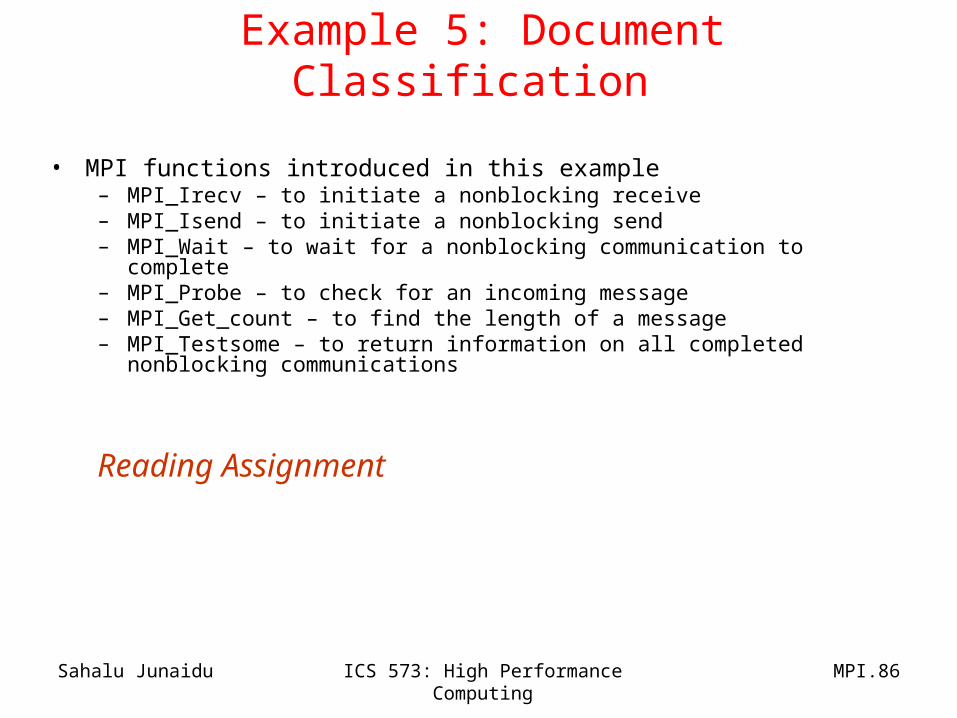
Example 5: Document Classification
• MPI functions introduced in this example– MPI_Irecv – to initiate a nonblocking receive– MPI_Isend – to initiate a nonblocking send– MPI_Wait – to wait for a nonblocking communication to complete– MPI_Probe – to check for an incoming message– MPI_Get_count – to find the length of a message– MPI_Testsome – to return information on all completed nonblocking
communications
Reading Assignment