Embed Size (px)
Citation preview

-
U i . SAND82-2772 * Unlimited Release a UC-70Printed June 1983
/4 Jt/4A
SAGUARO - A Finite ElementComputer Program for PartiallySaturated Porous Flow Problems
Roger R. Eaton, David K. Gartling, Don E. Larson
Prepared bySandia National LaboratoriesAlbuquerque, New Mexico 87185 and Livermore, California 94550for the United States Department of Energyunder Contract DE-AC04-76DP00789
C
0r-00
0n
z
rri
C.
Issued by Sandia National Laboratories, operated for the United StatesDepartment of Energy by Sandia CorporationNOTICE: This report was prepared as an account of work sponsored by anagency of the United States Government. Neither the United States Govern-ment nor any agency thereof, nor any of their employees, nor any of theircontractors, subcontractors, or their employees, makes any warranty, expressor implied, or assumes any legal liability or responsibility for the accuracy,completness, or usefunes of any information, apparatus, product, or pro-cess disclosed, or represents that its use would not infringe privately ownedrights. Reference herein to any specific commercial product, process, orservice by trade name, trademark, manufacturer, or otherwise, does notnecessarily constitute or imply its endorsement, recommendation, or favoringby the United States Government, any agency thereof or any of theircontractors or subcontractors. The views and opions expressed herein donot necessarily state or reflect those of the United States Government, anyagency thereof or any of their contractors or subcontractors
Printed in the United States of AmericaAvailable fromNational Technical Information ServiceUS. Department of Commerce5285 Port Royal RoadSpringfield, VA 22161
NTIS price codesPrinted copy- A06Microfiche copy A01

SAND82-2772 DistributionUnlimited Release UC-70Printed June, 1983
SAGUARO - A Finite Element Computer Programfor Partially Saturated Porous Flow Problems
Roger R. EatonDavid K. Gartling
Fluid Mechanics and Heat Transfer, Division 1511
Don E. LarsonAerodynamics Simulation, Division 1636
Sandia National Laboratories, Albuquerque, New Mexico 87185
ABSTRACT
SAGUARO is a finite element computer program designed to
calculate two-dimensional flow of mass and energy through porous
media. The media may be saturated or partially saturated.
SAGUARO solves the parabolic time-dependent mass transport
equation which accounts for the presence of partially saturated
zones through the use of highly non-linear material character-
istic curves. The energy equation accounts for the possibility
of partially-saturated regions by adjusting the thermal capaci-
tances and thermal conductivities according to the volume
fraction of water present in the local pores. Program capa-
bilities, user instructions and a sample problem are presented
in this manual.
i

CONTENTS
INTRODUCTION . . . . . . . . . . .
MATHEMATICAL FORMULATION . . . . .
PROGRAM FEATURES AND ORGANIZATION
INPUT GUIDE . . . . . . . . . . .
Header Card . . . . . . . . .
SETUP Command Card . . . . .
FORMKF Command Card . . . . .
OUTPUT Command Card . . . . .
UNZIPP Command Card . . . . .
STREAM Command Card . . . . .
HEATFLUX Command Card . . . .
PLOT Command Card . . . . . .
RESTART Command Card . . . .
Program Termination Card . .
Input Deck Structure . . . .
User Supplied Subroutines . .
Initial Conditions . . . . .
Error Messages . . . .
Page
. . . . . . . . . . . 1
...... . . . . . . . . ..... 3
...... . . . . . . . . ..... 7
* * . * .
. . . . .
. . .... . . .. 10
* . . .... . . .. .12
* . ..... ...... 12
* . . .... . . . .34
* . . .... . . .. .35
* . . .... . . .. .37
* . . .... . . ... 39
* . . .... .. . .41
* . . .... . . . .43
.... . * .... *.. 52
* . . .... . . . .54
. ..... ... . . .* 55
* . . .... . . .. .57
... . . ... *.. 69
.... . . ... * .. 71
* ...... . . . .75
* . ..... . . . .85
. ..... ..... * 86
... ... *.*.*.* 107
108
...... 110
v
* . . . .
Computer Requirements and Control Cards
A NOTE TO EXPERIENCED MARIAH USERS . . . . .
SAMPLE PROBLEM . . . . . . . . . . . . . .
REFERENCES . . . . . . . . . . . . . . . . .
APPENDIX A: CONSISTENT UNITS . . . . . .
APPENDIX B: DEGREE OF FREEDOM NUMBERING . .
ii

FIGURESPage
1. Characteristic Curves Relating HydraulicConductivity and Moisture Content toPressure Head for Sand/Soil; see reference . . . . . 5
2. Isoparametric Quadrilateral and TriangularElements . . . . . . . . . . . . . . . . . . . . . . 9
3. Notation for Orthotropic Materials . . . . . . . . . 18
4. Grid Point Generation Nomenclature . . . . . . . . . 23
5. Element Node Numbering and Side Numbering . . . . . 27
6. Control Card Deck -- Run with Plotting
a) CDC . . . . . . . . . . . . . . . . . . . . . . 79b) CRAY ... . . . . . . . . . . . . . . . . . . 80
7. Control Card Deck -- Run to Create a Restart Tape
a) CDC ... . . . . . . . . . . . . . . . . . . . 81b) CRAY ... . . . . . . . . . . ..... . . . 82
8. Control Card Deck -- Run with User Subroutines
a) CDC ... . . . . . . . . . . . . . . . . . . . 83b) CRAY . . . . . . . . . . . . . . . . . . . . . 84
9. Geometry Used in Sample Infiltration Problem . . . 86
10. Simplified Characteristic Curves for Sample Problem
a) Hydraulic Conductivity of Soil . . . . . . . . 87b) Moisture Content . . . . . . . . . . . . . . 88c) Derivative of Moisture Content with
Respect to Pressure Head . . . . . . . . . . . 88
11. Finite Element Grid for Sample InfiltrationProblem .* * * * *... . . . . . . .... . ....... 91
12. Initial Pressure Head . . . . . . . . . . . . . . . 92
13. Code Requirements for Sample Problem
a) Input Data . . . . . . . . . . . . . . . . . . . 93b) CDC 7600 Control Cards . . . . . . . . . . . . . 95c) CRAY Control Cards with Updating Done on
CDC 6600 ... . . . . . . . . . . . . . . .. . 95
iii
Page
14. User Subroutines for the One-DimensionalInfiltration Problem
a) Moisture Content and Derivative ofMoisture Content . . . . . . . . . . . . . . . . 96
b) Coefficient for Mass Transport . . . . . . . . . 96
c) Permeability . . . . . . . . . . . . . . . . . . 97
d) Thermal Conductivity . . . . . . . . . . . . . . 98e) Curve for Water Source . . . . . . . . . . . . . 98
15. Graphics Output from Sample Infiltration Problem
a) Effective Pressure as a Function of Timefor z = 0, 569, 814, 1113, 1267, and 1369 m. . . 99
b) Effective Pressure as a Function of Depthfor Time = 0, 2, 4, 6, 8 and 10 yr. . . . . . . 100
c) Temperature as a Function of Timefor z = 0, 569, 814, 1113, 1267 and 1369 m. . . 101
d) Temperature as a Function of Depthat Time = 0, 2, 4, 6, 8 and 10 yr ....... . 102
e) Velocity as a Function of Time for Z =0, 569, 814, 1113, 1267 and 1369 m. . . . . . . 103
f) Velocity as a Function of Depth at Time =0, 2, 4, 6, 8 and 10 yr.. . . . . . 104
g) Moisture Content as a Function of Time forZ = 0, 569, 814, 1113, 1267 and 1369 m. . . . . 105
h) Moisture Content as a Function of Depthat Time = 0, 2, 4, 6, 8 and 10 yr. . . . . . . . 106
iv

Nomenclature
Typical Units
CCP
Di jEij
Jhki.
K
ppQtTv
Vx
yz
AeXij£
P
4,
- specific heat- specific moisture capacity (6B/af)- themal diffusion tensor (Soret)- thermal dispersion tensor- gravitational constant- heat transfer coefficient- intrinsic permeability tensor
- hydraulic conductivity (kpg)
- effective pressure = pog (f + z)- pressure- volumetric heat generation- time- temperature- Darcy velocity (Mean Specific flux, m3 /sm 2 )- volumetric heat generation rate- horizontal dimension- vertical dimension- vertical dimension- coefficient of volumetric thermal expansion- increment- moisture content- thermal conductivity tensor- emissivity- dynamic viscosity- liquid density- Stefan-Boltzmann constant- porosity
- pressure head (p)
*ipts
effective propertyfluidcoordinate directionreference conditionsolid property
J/kg6Kl1/m
m 2 /s eKJ/smK
m/s 2
J/sim2 .Km
m/s
N/m 2
J/m *ss°K
m/sJ/s Om3
mmm
kg/m 3 K
J/s -m-K
kg/m-skg/m3
4) m
Subscr
efffi, }o, rs
v-vi
INTRODUCTION
Recent interest in the potential performance of a nuclear-
waste repository located above the water table in tuff (a hard
rock) has prompted the development of a computational code,
SAGUARO.* SAGUARO is a general-purpose finite element code
developed to solve problems of incompressible single phase
water and energy transport through porous media which may be
partially or fully saturated. The two transport equations
(mass and energy), which model the flow, incorporate Darcy's
law, the Boussinesq approximation, the Soret effect, conduc-
tion and convection. The resulting nonlinear parabolic equa-
tions are solved in finite-element form using an algorithm
related to the standard Crank-Nicolson method. The matrix
solution procedure used in SAGUARO is a form of Gauss elimina-
tion. Code results provide time and space distributions of
hydraulic head, temperatures, velocities and moisture contents.
SAGUARO is the newest member of the family of codes NACHOS,'
COYOTE,2 and MARIAH3 which employ a similar structure. SAGUARO
represents a direct extension of MARIAH (which solves problems
of fully saturated flow in porous media) in that the quasi-steady
state continuity/momentum equation in MARIAH was replaced with a
transient equation which allows some or all of the pore volume to
be partially saturated with water. The resulting equation is
*The Nevada Nuclear Waste Storage Investigations Project, managedby the Nevada Operations Office of the U.S. Department of Energy,is examining the feasibility of siting a repository for high-level nuclear wastes at Yucca Mountain on and adjacent to theNevada Test Site. This work was funded in part by the NNWSIProject. The ultimate use of this information will be used forsystem analysis and performance assessment of a nuclear wasterepository in tuff.
1
similar to Richards equation5 commonly used to solve near-surface
isothermal hydrology problems. The general form of the energy
equation remains the same except that coefficients now depend on
the degree of saturation.
The structure of SAGUARO and MARIAH are identical in the
areas of grid generation, element basis functions, quadrature
schemes, solution methods and plot packages. Therefore, the
layout of this manual closely parallels the report describing
MARIAH. The user may refer to that manual for additional
information regarding the general code structure and solution
procedure.
2
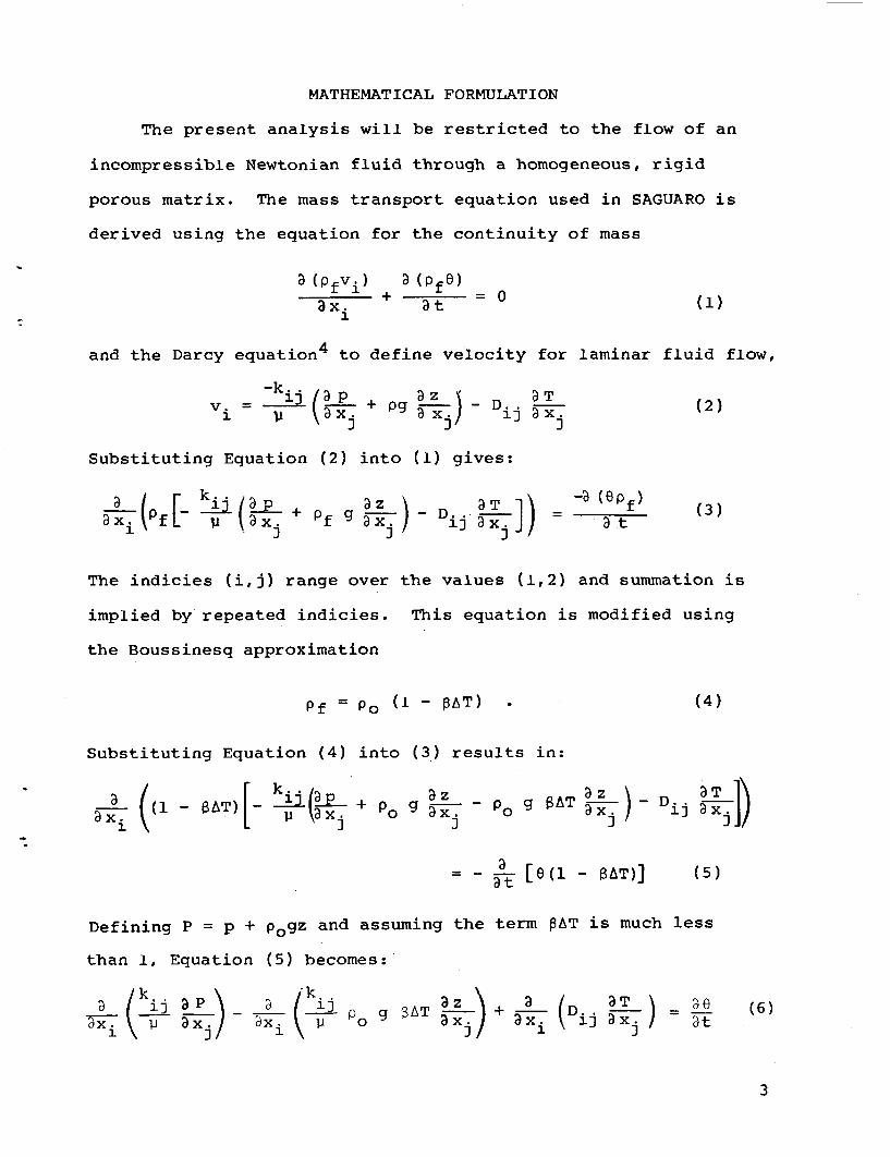
MATHEMATICAL FORMULATION
The present analysis will be restricted to the flow of an
incompressible Newtonian fluid through a homogeneous, rigid
porous matrix. The mass transport equation used in SAGUARO is
derived using the equation for the continuity of mass
a (pfvi) a (PfO) )ax. + at
1
and the Darcy equation4 to define velocity for laminar fluid flow,
-k.Vi =api]/ P. + pg az Dj DT (2)
1 (~axi axi) (2) ax
Substituting Equation (2) into (1) gives:
a Lp[_ kID(3p az D T -a (ePf) (3)ax.( \ 1f pax. + Pf g ax. ax.' at
The indicies (i,j) range over the values (1,2) and summation is
implied by repeated indicies. This equation is modified using
the Boussinesq approximation
Pf = pO (1 - PAT) . (4)
Substituting Equation (4) into (3) results in:
((1 - A)-9ax. gfaxa.((1 - «AT)L ii~ax. + p g az _ PO g iAT -) j Xax1 J i
- - a [e(1 - EAT)] (5)
Defining P = p + pogz and assuming the term PAT is much less
than 1, Equation (5) becomes:
(ak.. 1 k). a +- 7 1309 A + a (D~ axT .Di (6)
3

Since the air is assumed to be free to escape at the surface,
the air pressure is small in comparison to the liquid pressure p.
Thus the liquid pressure is simply the negative of the capillary
pressure PC:
P PC(9) (7)
This can be inverted to yield a representation of the moisture
content e as a function of liquid pressure p or pressure head
q, whichever is desired, and its slope C = is the specific
moisture capacity. Thus, using the chain rule, (6) and (7) yield
the final form of the parabolic equation which is solved in
SAGUARO
Us ( ]a s %PO g BAT a-) + a3 (Di aT
1 _ aPg cat (8)
In general, mass transport in partially saturated regions,
resulting from bouyancy effects, is expected to be negligible.
This fact is accounted for by setting l E 0 when 0/¢ is less 99%.
It is of interest to note two special cases of Equation (8).
For saturated flows, the moisture content is constant (6/4 = 1) 4
therefore, 0. Typically, mass transport resulting from
a am 3temperature gradients, a Dia - , is much smaller than mass
ax ij x.transport resulting from pressure gradients. For these condi-
tions, the third and fourth terms in Equation (8) are neglected
yielding an equation for flow through fully saturated media,
ax. ( > ax. ax. ( l ax 9
4

f
This equation, which is elliptic in nature, is the equation
solved by MARIAH.
For isothermal flows, the second and third terms of Equation
(8) vanish, leaving
a 1 -aPA= - C LP (10)axi \j a axi Pog at
This is the well-known Richards equation.5
For partially saturated flow, the properties kij, Dij and
C are strong functions of pore pressure. Thus Equation (8) is
highly non-linear. Generally, the non-linear coefficients
k(4,) and C(4f) are functions of 4, similar to the typical
curves shown in Figure 1. The curves show the significance
of the hystersis effects on the k(q,) and 0(4,) relationship.
These curves account for the influence of capillary action.
Note K(4,) = kpg/p.
- - Unsoturotedv-iea Soturoted
qTgnsio-sotulruted -. _I SatuioSidI moistute
0~~ymg ~ content 30D~rying75 * porosity Si * 0.03
-400 Wettin - 20-oi 010-40-0-20-100l1l0
PriCure heod, + lem of Toter) Ple~u t hbod, + {m of woter)
{~~~~o soil
£0)~~~~-2
Figure 1: Characteristic Curves Relating Hydraulic Conductivityand Moisture Content to Pressure Head for Sand/Soil,see Reference 5.
5

The general form of the energy equation solved by SAGUARO
is,
(PC ) faT+ P (C ) Vp eff at 4, p fi ax.1
axi [(effij _- Eij) x ] Q = 0 * (11)
This equation is an energy balance on a unit volume containing
a porous matrix and liquid and neglects the heat capacity of
the air. It is further assumed that the matrix and liquid are
in thermal equilibrium. Both energy transport by convection
(2nd term) and conduction/dispersion (3rd term) are included.
However, the definitions of the coefficients of the terms must
be defined to allow the possibility of partially saturated
pores. These coefficients are therefore defined as follows:
(pc) eff = ePf(C )f + (l 4) Ps (Cp)s I (12)
where (pc)eff represents the thermal capacitance of a unit
volume with porosity (f), saturation (0/Q), and
eff Xf + ( -) X + (1 -)X 5 , (13)ij airf 4 x ]
where Xeff is the effective conductivity of the water, air,
solid combination.
6
PROGRAM FEATURES AND ORGANIZATION
SAGUARO is restricted by the following limitations and
assumptions.
(a) The geometric description of the problem is limited to two
spatial dimensions, either plane or axisymmetric.
(b) The porous matrix is assumed to be homogeneous and rigid.
The matrix material may be considered orthotropic in terms
of thermal conductivity, permeability and thermal diffusion.
(c) The matrix materialts) is assumed to be saturated or partially
saturated with a single, one-phase fluid (no vapor transport).
The fluid is assumed to be incompressible and Newtonian.
(d) The fluid flow is assumed to be laminar. Inertia effects
in the fluid are assumed negligible.
(e) For non-isothermal flows, the fluid and material matrix
are assumed to be in local thermal equilibrium.
(f) Presence of air in momentum/continuity equation is neglected.
Despite these restrictions, SAGUARO has proved to be a use-
ful tool in the solution of a wide range of transient porous flow
problems. When considering flows with heat transfer, regions
of solid body heat conduction are easily included in the analy-
sis. Material properties such as fluid viscosity and thermal
conductivity may be arbitrary functions of temperature; volu-
metric heat sources may be functions of time and/or temperature.
Allowable boundary conditions on the hydrological and thermal
parts of a problem are quite general and may include the specifi-
cation of the fluid hydraulic head or hydraulic head gradient
(fluid discharge), as well as specified temperatures, heat fluxes
7

or convective and radiative boundaries. All boundary conditions
may be functions of time.
SAGUARO is a self-contained program with its own mesh
generator, data analysis, and plotting packages. The mesh
generator is based on an isoparametric mapping procedure and
allows very general meshes to be prepared easily and accurately.
The data analysis portions of the code allow local heat fluxes
as well as stream function values to be calculated. The
plotting package provides graphic output of element meshes,
nodal point locations, contour plots of temperature, hydraulic
head, or stream function, profile plots, and time histories of
any dependent variable.
Two other essential parts of the SAGUARO code are the
element library and the solution procedures for the matrix
equations. The elements included in SAGUARO consist of iso-
parametric and subparametric quadrilaterals and triangles as
shown in Figure 2. Within each of these elements, the hydraulic
head and temperature are approximated using biquadratic basis
functions; the velocity components are expressed by a bilinear
basis function. Transient problems are analyzed using a
modified Crank-Nicholson procedure. The actual solution of
the matrix equations is carried out by a specialized form of
Gauss elimination.7 These procedures are fully described in
References 3 and 4.
8

v I
P.T
P,Tu,v
P,T
PT PT PT
Uv UV
FIGURE 2. Isoparametric Quadrilateral and Triangle
.0

INPUT GUIDE
The structure of an input data deck for the SAGUARO
computer code directly reflects the steps required to formulate
and solve a finite element problem. Through the use of a
series of command and data cards, the program is directed to
such functions as grid generation, element construction,
solution of the matrix equations, and calculation of auxiliary
data. The actual sequence of commands to the program is quite
flexible, although there are some obvious limits to the order in
which operations can be specified. In the following sections,
the command and data cards required by SAGUARO are described in
roughly the order in which they would normally appear in an
input deck. An example problem follows this section as an
added aid to input format. Additional example problems for
fully saturated cases can be found in Reference 1.
In the following section, the conventions listed below
are used in the description of input cards:
(a) Upper case words imply an alphanumeric input value,
e.g., FORMKF.
(b) Lower case words imply a numerical value for the
specified variable, e.g., xmax.
(c) All numerical values are input in a free field
format with successive variables separated by
commas. All input data is limited to ten
characters under this format for the CDC machine
and eight for the CRAY version.
10

(d) [l indicate optional parameters which may be omitted
by using successive commas in a variable list. If
the omitted parameter is not followed by any re-
quired parameters, no additional commas need to be
specified.
(e) <> indicates the default value for an optional
parameter.
(f) The * character may be used to continue a variable
list onto a second data card. When using this
option the comma following the last variable and
preceeding the * is omitted.
(g) The $ character may be used to end a data card
allowing the remaining space on the card to be
used for comments.
(g) The contents of each input card are indicated by
underlining.
(i) All quantities associated with a coordinate
direction are expressed in terms of the planar x-y
coordinate system. The corresponding quantities
for axisymmetric problems are obtainable from the
association of the radial coordinate, r, with x and
the axial coordinate, z, with y.
The description of the command cards are presented in the
following order:
(a) Header Card
(b) SETUP Command Card
(c) FORMKF Command Card
11

(d) OUTPUT Command Card
(e) UNZIPP Command Card
(f) HEATFLUX Command Card
(g) PLOT Command Card
(h) RESTART Command Card
(i) Program Termination Card
Following the individual descriptions of the command cards
are sections discussing input deck structure, user subroutines,
initial conditions, error messages, and computer requirements
for SAGUARO.
Header Card
The header card must be the first card in a deck for any
particular problem. If two or more problems are run in sequence,
the header card for each new problem follows the END, PROBLEM
card of the previous problem. A $ symbol must appear in Column
1; the remaining 79 columns are available for a problem title.
The header card is of the following form:
$ PROBLEM TITLE.
SETUP Command Card
The first task in formulating a finite element analysis
of a problem involves the specification of the material pro-
perties and the definition of element mesh and boundary condi-
tions for the problem geometry. These functions are accomplished
through the SETUP command and its three sets of associated data
cardso
The SETUP command card has the following form:
12

SETUP, [iprint], [maxi], [order], [grid plot]
where,
iprint <2>: determines the amount of printout produced
during the setup operation. Output increases with the
value of iprint and ranges from no printout for iprint =
1 to full printout for iprint = 4.
maxi <18>: is the maximum number of I rows to be generated
in the grid. Maxi need only be specified if there are
more than 18 I rows or more than 110 J rows. The limit
on the maximum I's and J's is I*J < 4000 for the CDC
version of SAGUARO and I*J 4 5000 for the Cray version.
order < >: determines the numbering of the elements.
For the default value (i.e., order left blank), the
elements are numbered by increasing I,J values (e.g.,
(1,1), (2,1), (3,1) ... (1,2), (2,2) ... ). For
order = PRESCRIBED, the elements are numbered according
to their order in the input list. The element ordering
should be chosen such that the front width of the pro-
blem is minimized.
grid plot < >: determines if a grid point plot tape is
written. If a plot of the grid points is to be made in
a subsequent call to the plot routine, then grid plot =
PLOT; if no plot of the grid points will be made, the
grid plot parameter is omitted.
SETUP Data Cards
Following the SETUP command card, three sets of data cards
are required for material property specification, grid point
13

generation, and element and boundary condition specification.
Each of the data sets is terminated by an END card. The last
END card (i.e., the third), ends the setup portion of the program
and readies the program for the next command card.
Material Data Cards
The material data cards are of two types corresponding to
the specification of fluid and matrix (solid) properties, res-
pectively. For the specification of the fluid properties, the
data cards are of the following form:
[Material Name], number, Pf'? Pf, Cf, Xf,
i, g, temperature dependence, Tref
where,
Material Name: is an optional alphanumeric material name for
user reference.
number: is the internal reference number for the material.
For the fluid property card, number must be set to 1.
pf: is the fluid density.
pf: is the fluid dynamic viscosity.
cf: is the fluid specific heat.
Xf: is the fluid thermal conductivity
i: is the fluid volumetric expansion coefficient
(= pE8(l/p)/8T]p = -(l/p) Ep/6T]).
g: is the gravitational acceleration.
Temperature dependence <CONSTANT>: prescribes the depen-
dence of the fluid properties on temperature. If all
fluid properties (p, X, and p) are independent of
temperature, this parameter is omitted or set equal
14

to CONSTANT. If one or more the indicated properties
depend on temperature, this parameter is set equal to
VARIABLE.
Tref <0>: is the reference temperature for the buoyancy
force, i.e., Tref is the temperature at which the buoyancy
forces are zero.
The material properties for the matrix are specified on data cards
of the following form:
[Material Name], number P., Cs, k11 , X22, ax#
*, k 1l, k22, ak, dispersion, temperature dependence
S, Tint, Pint
UNSAT, number, D11, D22, aD1 C, SAT, hair
where,
Material name: is an optional alphanumeric material name
for user reference.
number: is the internal reference number for the material.
SAGUARO will accept up to ten materials; the materials
must be numbered such that 2 < number < 11.
ps: is the material density.
cs: is the material specific heat.
X11, X22<X11>: are components of the material thermal
conductivity tensor (see below).
aX<O>: is the angle in degrees between the principle
material axes (for conductivity) and the coordinate axes
(see below).
51

0: is the material porosity. For * set to zero,
the material is treated as impermeable.
kll, k2 2 <kll>: are components of the material permea-
bility tensor for the saturated state of the material.
ak<0°>: is the angle in degrees between the principle
material axes for permeability and the coordinate
axes (see below).
dispersion <NONE>: prescribes the use of a model for
hydrodynamic dispersion. If no dispersion is to be
included in the analysis, this parameter is omitted or
set equal to NONE. If a dispersion model is to be
included, this parameter is set equal to VARIABLE.
temperature dependence <CONSTANT>: prescribes the de-
pendence of the material properties on temperature time,
location, etc. If all material properties (Xii, kii)
are invariable, this parameter is omitted or set equal
to CONSTANT. If one or more of the properties depend
on temperature (or any other variable, e.g., hydraulic
head or spatial location), this parameter is set equal
to VARIABLE.
S<O>: is the volumetric heat source for the material. For
no volumetric heating, this parameter is omitted; for
constant volumetric heating, the parameter is set equal
to the heating value. If the heat source varies with
location, time or temperature, this parameter is set
equal to VARIABLE.
'16
Tint <0>, Pint<O>: specify the values of the initial tem-
perature and effective pressure for the material. Note
Pint = p + pgz where p is the pore fluid pressure.
UNSAT: First word on current line of data. Inserting
this data card implies that the user wishes to define
constant values for Dll, D22, aDl C, SAT and kair*
If temperature dependence is set equal to VARIABLE then
the coefficients Dll, D2 2 , aD, C, SAT and kair need
to be defined in user supplied subroutines. If this
card is omitted, Dll, D22, aD, and C will be initialized
to zero. SAT will be set to one. If these values are
appropriate for the calculation then this card can be
omitted.
Number: This internal material reference number must agree
with the material number on the preceeding material data
card.
Dll, D22<Dll>: Thermal mass diffusion coefficient (see
equation 10).
aD<0°>: is the angle in degrees between the principle
material axis for thermal mass diffusion and the coordi-
nate axis.
C: (Equation (10)) coefficient of time derivative
term in the mass transport equation.
SAT: Saturation (moisture content/porosity);
(unsaturated) 0 < SAT < 1.0 (fully saturated).
kair: Thermal conductivity of air (or any gas) in porous
medium.
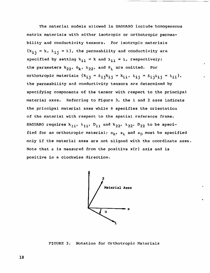
The material models allowed in SAGUARO include homogeneous
matrix materials with either isotropic or orthotropic permea-
bility and conductivity tensors. For isotropic materials
(kij = k, Xij = X), the permeability and conductivity are
specified by setting kil = k and Xi, = X, respectively;
the parameters k22, ek, X22, and ok are omitted. For
orthotropic materials (kij = 6ijkij = kii, Xij = 6ijxij =ii),
the permeability and conductivity tensors are determined by
specifying components of the tensor with respect to the principal
material axes. Referring to Figure 3, the 1 and 2 axes indicate
the principal material axes while 0 specifies the orientation
of the material with respect to the spatial reference frame.
SAGUARO requires k11, X 11, D11 and k22, X22, D22 to be speci-
fied for an orthotropic material; ak, aX and aD must be specified
only if the material axes are not aligned with the coordinate axes.
Note that a is measured from the positive x(r) axis and is
positive in a clockwise direction.
2
Material Axes
x
FIGURE 3. Notation for Orthotropic Materials
18

The variation of material and fluid properties with tempera-
ture, the specification of a hydrodynamic dispersion model and
the variation of the volumetric heating with time and/or tempera-
ture is indicated by setting the parameters "temperature depend-
ence," "dispersion," and "S" equal to VARIABLE, respectively.
The actual variation of these quantities is specified by several
user supplied subroutines. If temperature dependent properties
have been specified, SAGUARO requires subroutines VISCOUS, ISOVOL,
FLUIDC, DIF, PERM, FLAMBDA, and SLAMBDA to be supplied by the user.
The inclusion of a dispersion model requires Subroutine DSPERSE
to be provided; a variable heat source requires Subroutine SOURCE.
Further details on these subroutines are given in a later section
of this chapter. Note that when variable properties have been
specified, all appropriate property values must still be supplied
on the material data card. These values are used as initial
estimates for the material properties when problems with material
nonlinearities are being considered.
SAGUARO does not contain any dimensional constants and,
therefore, the units for the material properties are free to
be chosen by the user. For convenience, a table of consistent
units is given in Appendix A.
Grid Data Cards:
Following the material specification, the grid points
for the finite element mesh are generated. In contrast to
many finite element codes, SAGUARO separates the generation
of nodal points and the generation of elements into distinct
operations. The calculation of nodal point locations is
19
accomplished by use of an isoparametric mapping scheme that
considers quadrilateral parts or regions of the problem domain
separately. For each part, a series of coordinates are speci-
fied which determine the shape of the region boundary. The
node points within each part are identified by an I, J number-
ing system. The location of points in a region is controlled
by user specification of the number of points along a boundary
side and a local gradient parameter. These ideas are more
clearly fixed through a description of the data cards required
to generate points in a part.
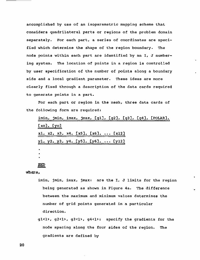
For each part or region in the mesh, three data cards of
the following form are required:
imin, jmin, imax, jmax, [gl], Eg2], [g3], [g4], [POLAR],
Exo), [yo]
xl, x2, x3, x4, [x5], [x6], ... [x12]
yl, y2, y3, y4, [y5], Cy6], ... [yl2J
..w: ae,
imin, jmin, imax, jmax: are the I, J limits for the region
being generated as shown in Figure 4a. The difference
between the maximum and minimum values determines the
number of grid points generated in a particular
direction.
gl<l>, g2<l>, g3<1>, g4<l>: specify the gradients for the
node spacing along the four sides of the region. The
gradients are defined by
gi or g3 = node spacing at imin = Aiminnode spacing at imax iima-x
g2 or g4 = node spacing at jmin = Ajminnode spacing at jmax &jmax
and are illustrated in Figure 4a. The default values
of unity give equal node spacing along a side. Gra-
dients either larger or smaller than unity may be used
to bias the spacing in either direction.
POLAR, xo<O>, yo<O>: specify the use of polar coordinates
for describing the coordinates of the points defining
the region. With POLAR specified, the x's and y's on
the second and third data cards are interpreted as polar
radii and angles referred to the local origin xo, yo.
The polar angle is referenced to the positive x axis;
positive angles are measured in a counterclockwise
direction.
xl, x2, ... x12: define the coordinates of the four corner andyl, y2, ... y12:
optional side nodes for each part. If the region is
bounded by straight lines, only the four corner coordinate
(i.e., xl to x4 and yl to y4) need be specified. If any
of the region sides are curved, then the appropriate
side nodes, as shown in Figure 4b must be specified. If
one side node is defined, a quadratic interpolation is
used to define the boundary; specification of two side
nodes allows a cubic interpolation. Side nodes should
be located near the midside and one-third points for
quadratic and cubic interpolation, respectively.

There are no limits on the number of parts which may be used
to define a grid. The only restriction on the total number of
grid points is that max (I*J) 4 4000 for the CDC version of
SAGUARO and max (I*J) 4 5000 for the Cray version.
Node points may be generated for a triangular shaped region
by allowing two adjacent corners of the quadrilateral part to
coincide. However, when triangular meshes are created in this
manner, the location of interior node points is generally un-
predictable. The user is advised to verify the quality of such
a mesh through use of a node point plot.
In generating mesh points for complex geometries, it is
often convenient to be able to position an individual node
point or a line of nodes. These situations are provided for
in SAGUARO by use of the following data cards:
POINT, i, j, xl, yl, [POLAR], [xo], [yo]
where,
i,j: is the I, J name for the point.
xl,yl: are the coordinates for the point.
POLAR, xo<O>, yo<O>: specify the use of polar coordi-
nates as described previously.
ARC, imin, jmin, imax, jmax, [gl], [POLAR], Exo], [yo]
xl, x2, [x3], [x4]
yl, y2, [y3], [y4]
wb rv0,
imin, jmin, imax, jmax: are the I, J limits for the arc
as shown in Figure 4c. Since a one-dimensional array
22

Side 393
imax, Jmax
imin, jmax
Side 4g4
x4,y4 1
x8,y8 1
(a) I, J Nomenclature
7 x3,y3
xlOylO
x12
xl,yl
(b) Coordinate Nomenclature
imax, irminx2,y2
W--- x 3, y 3 x4,y4imin, joinxl,yl
(c) ARC Nomenclature
FIGURE 4. Grid Point Generation Nomenclature

of points is being generated, either imin = imax or
jmin = jmax. The difference between the maximum and
minimum values determines the number of grid points
generated along the arc.
gl<l.O>: specifies the gradient for the node spacing
along the arc.
The gradient is defined by
gl = node spacing at ijmin = Aijminnode spacing at ijmax Aijmax
and is illustrated in Figure 4c.
POLAR, xo<O>, yo<O>: specify the use of polar coordinates
as described previously.
xl, x2, x3, x4: define the coordinate for the ends ofyl, y2, y3, y4:
the arc and the optional intermediate points. If the arc
is a straight line only the first two coordinates need be
specified. The generation of a curved arc requires the
specification of one or two intermediate points as shown
in Figure 4c.
There are no limits on the number of POINT and ARC data cards
that may be used in generating a mesh. Both types of cards may
appear at any point within the grid point data section of the
SETUP command.
EXTDEF
This data card causes the user supplied Subroutine EXTDEF
to be called by the mesh generator. Within this subroutine,
the user may create an arbitrary array of I, J labeled nodal

points. The EXTDEF data card may be used in conjunction with
the standard nodal point generation schemes or may be used to
create an entire mesh. The data card may appear at any appro-
priate point within the grid point data section of the SETUP
command. Details on the form of Subroutine EXTDEF are given
in a later section.
Element and Boundary Condition Data Cards:
Following the generation of the grid points, the program
is ready to accept element and boundary condition data. Since
the mesh points for the problem geometry are generated inde-
pendently of the elements, the selection of nodes from which
to construct a given element is very flexible. The actual
construction process for an element consists of identifying
an appropriate group of previously generated mesh points that
will serve as the corner and midside nodes of the element.
This concept is apparent from the form of the element data
card.
element type, mat, il, jl, [i2], [j2), ... [in], [jn]
where,
element type: is an alphanumeric name for the type of
element. The element types used in SAGUARO are
described below.
mat: is the matrix material number for the element.
This number should be set to correspond to the matrix
material number used on the material property card
(2 4 mat < 11).

il, jl, [i2], [j2), ... : is the list of I, J values for
the node points in the element. The nodes of an ele-
ment are listed counterclockwise around the element
starting with any corner as shown in Figure 5. In
some situations, the list of I, J values may be signi-
ficantly condensed. When only the first node, I, J
values are specified for a quadrilateral element, the
following values for the remaining nodes are assumed,
i4 = i8 = il, i5 = i7 = il + 1, i2 = i3 = i6 = il + 2
j2 = j5 = jl, j6 = j8 = jl + 1, j3 = j4 = j7 = jl + 2
When I, J values are specified for only the corner nodes
of any element, the midside I, J values are computed as
the average of the corner values.
The specification of different types of elements is pro-
vided by the "element type" parameter on the previously des-
cribed data card. The permissible element names for this para-
meter include the following:
(a) QUAD8/4 -- A subparametric quadrilateral with
arbitrarily oriented straight sides.
(b) QUAD8/8 -- A general isoparametric quadrilateral
with quadratic interpolation used to define the
shape of the element sides.
(c) TRI6/3 -- A subparametric triangle with arbitrarily
oriented straight sides.
(d) TRI6/6 -- A general isoparametric triangle with
quadratic interpolation used to define the shape of
the element sides.
26
3
6
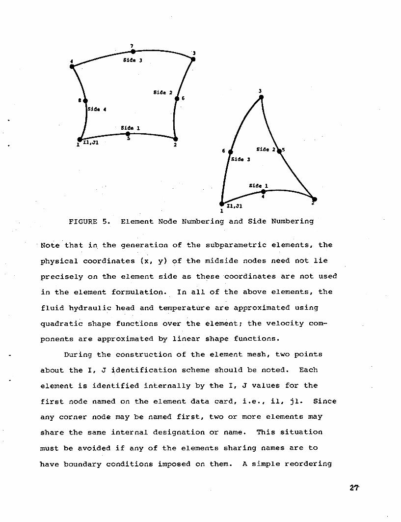
FIGURE 5. Element Node Numbering and Side Numbering
Note that in the generation of the subparametric elements, the
physical coordinates (x, y) of the midside nodes need not lie
precisely on the element side as these coordinates are not used
in the element formulation. In all of the above elements, the
fluid hydraulic head and temperature are approximated using
quadratic shape functions over the element; the velocity com-
ponents are approximated by linear shape functions.
During the construction of the element mesh, two points
about the I, J identification scheme should be noted. Each
element is identified internally by the I, J values for the
first node named on the element data card, i.e., il, jl. Since
any corner node may be named first, two or more elements may
share the same internal designation or name. This situation
must be avoided if any of the elements sharing names are to
have boundary conditions imposed on them. A simple reordering
2a

of the nodes in the appropriate elements remedies this
situation. Secondly, during the generation of grid points,
there is no requirement that adjacent parts of the grid have
a continuous I, J numbering. When elements are constructed
along boundaries of such adjacent parts of the grid, it is
imperative that common nodes between elements have the same
I, J values. Element connectivity is generated from the I, J
values for each node and, therefore, common nodes with
different I, J labels will not be properly connected. The
generation of element meshes using node points with non-
continuous I, J labels is illustrated in the example section.
The boundary conditions for the problem are specified by
element and may appear at any point in the present data sec-
tion after the element to which they apply has been defined.
Boundary conditions are specified to have either a constant
value along an element side or a particular value at a node.
The boundary condition data card has the following form:
BC, b.c. type, il, jl, side/node, value/set no./time curve no.
where,
b.c. type: is an alphanumeric name for the type of
boundary condition. The types of boundary conditions
used in SAGUARO are described below.
il, jl: is the I, J identification of the element
(i.e., the first I, J named on the element data card)
to which the boundary condition applies.
side/node: identifies the side or node of the element

to which the boundary condition is to be applied. The
numbering of nodes and sides begins with the identifying
node (i.e., the first node named on the element data
card) and proceeds counterclockwise as shown in Figure 5.
value/set no./time curve no.: is the numerical value of the
applied boundary condition, the number of the boundary con-
dition SET in the case of convective or radiative boundary
condition, or the number of the time history curve for
time dependent boundary conditions. For specified pres-
sure, velocity, temperature, or heat flux boundary con-
ditions, this parameter is set to the numerical value
of the boundary condition. The specification of a set
or time curve no. is explained below.
The permissible type of boundary conditions as speci-
fied by the parameter "b.c. type" include the following:
(a) P -- specifies the effective pressure at a node.
(b) PSIDE -- specifies the hydraulic head to have a
constant value along an element side.
(c) PVARY -- specifies the hydraulic head along an element
side to be a function of time.
(d) USIDE -- specifies the fluid velocity (volumetric
flow/unit area) normal to the element boundary to
have a constant value.
(e) UVARY -- specifies the fluid velocity (volumetric
flow/unit area) normal to the element boundary to
be a function of time.
219

(f) T -- specifies the temperature at a node.
(g) TSIDE -- specifies the temperature to have a con-
stant value along an element side.
(h) TVARY -- specifies the temperature along an
element side to be a function of time.
(i) QSIDE -- specifies a constant heat flux (energy/
unit area/unit time) along an element side.
(j) QVARY -- specifies a time dependent heat flux
along an element side.
(k) QCONV -- specifies a constant convective heat
transfer process along an element side.
(1) QRAD -- specifies a radiative or temperature
dependent convective heat transfer process along
an element side.
(m) Impermeable surface -- no boundary condition need
be applied.
(n) Adiabatic surface -- no boundary condition need
be applied.
All of the above boundary conditions can be employed with any
of the previously described elements.
The boundary condition options, PVARY, UVARY, TVARY, and
QVARY permit hydraulic head, fluid velocity, temperature or heat
fluxes along an element boundary to vary with time. The time
histories of the boundary condition are input through a set
of user supplied subroutines (Subroutine CURVEn). The asso-
ciation of a particular time history with the appropriate
boundary condition is accomplished by use of the "time curve
30

no." which appears on the boundary condition data card and in
the user supplied subroutine name. SAGUARO will allow a total
of six different time histories to be input. The format for the
time history subroutines is described in a subsequent section.
The use of convective and radiative boundary conditions
requires the appropriate heat transfer coefficients (he, hr)
and reference temperatures (Tc, Tr) to be specified. These
parameters are input through use of a SET data card which is
of the form:
SET, b.c. type, set no., h, T
where,
b.c. type: is the alphanumeric name of the type of
boundary condition for which data is being specified,
i.e., either QCONV or QRAD.
set no.: is the number of the particular data set.
The code allows up to ten data sets for each type of
boundary condition. The set no. is used to identify
the appropriate boundary condition set on the BC card.
h, T: are the parameters required for specifying a convec-
tive or radiative boundary condition. For convection,
h = heat transfer coefficient = hc and T = Tc. For
fourth power radiation, h = emissivity, Stefan-Boltzmann
constant = E*oa and T = Tr. For generalized radiation/convection,
h = VARIABLE and T = Tr. The generalized radiation/convection
condition mentioned above has been provided to allow an arbi-
trary variation of h with temperature or time in the flux
expression,
31i~

q = h(T, x, y, t)(T - Tr) -
To incorporate such a boundary condition, the parameter "b.c.
type" must be set to QRAD, "h" must be set to VARIABLE, "T" is
set to the appropriate reference temperature, and the user
supplied subroutine HTCOEF, which describes h(T, x, y, t),
must be appended to the SAGUARO program. This subroutine is
described in detail in a later section of this chapter.
The SET data cards may appear anywhere in the present
data section; SET cards for both types of boundary condition
may appear in the same problem.
Looping Feature:
In order to permit easy specification of elements and
boundary conditions which appear in regular patterns in the
mesh, a looping feature is incorporated in SAGUARO. This
feature allows the definition of ILOOP's and JLOOP's (which
are similar to FORTRAN DO loops) for incrementing data in
the I and J directions. Nesting of the loops may be in any
order but no more than one loop in a given direction may be
used at one time. Note that within each loop all the I
(or J) values are given the same increment. The looping
commands are of the following form:
ILOOP, npass, inc. or JLOOP, npass, inc.
element or boundary element or boundarycondition data cards condition data cards
32

IEND JEND
where,
npass: specifies the number of passes to be made through
the loop.
inc: specifies the increment to be added to the I or J
values found within the loop. the "inc" parameter may
be negative.
The looping commands may appear at any point within the
element and boundary condition data section of the SETUP command.
The use of the looping feature is illustrated in the example
problem.
II3

FORMKF Command Card
With the completion of the SETUP command, the next task
in the analysis sequence is the formulation of the matrix
equations for the individual elements in the mesh. This
function is carried out by the command card:
FORMKF, [geometry], [type of flow], [vel. comp.]
'her-e,
geometry: is an alphanumeric name to indicate the type
of coordinate system desired. If geometry is omitted,
the two-dimensional planar formulation is used; if
geometry = AXISYM, the axisymmetric formulation is
used.
type of flow: is an alphanumeric name to indicate the
type of problem being considered. If type of flow is
omitted, the problem is treated as an isothermal flow
problem. Forced convection heat transfer problems
are designated by setting type of flow = FORCED.
Free convection or mixed convection problems are
indicated by setting type of flow = FREE.
vel. comp.: is an alphanumeric name to indicate the
type of velocity computation that will be used in the
analysis. If vel. comp. is omitted, the velocity field
will be computed on an element basis which results in a
discontinuous velocity field. If vel. comp. = CONTINUOUS,
the velocity field will be computed from a global matrix
equation which results in a continuous velocity field.
3:4
OUTPUT Command Card
Prior to solution of the porous flow problem, it is some-
times convenient to limit the amount of printed output gener-
ated by SAGUARO. It may also be desirable to specify spatial
locations within the mesh other than nodal points at which
output of the dependent variables is required. Both of these
functions may be invoked through use of the OUTPUT command card.
The selective printing of the computed dependent variables may
be set up through use of the following command card:
OUTPUT, delimiter type, nl, n2, n3, ... n50
where,
delimiter type: is an alphanumeric name to indicate how
the subsequent element numers are to be interpreted
in limiting the printed output. If delimiter type
SINGLE, individual element numbers are assumed to be
listed in the following data. If delimiter type =
STRING, the following data is interpreted as pairs of
element numbers with each pair defining a sequence
of elements.
nl, n2 ... n50: is a list of element numbers indicat-
ing which elements are to have flow field data
printed during the solution process. A maximum of
fifty individual element numbers or twenty-five
element pairs may be specified on a single command
card.
3a!
There is no restriction on the number of OUTPUT command
cards that can be used in a SAGUARO input deck; OUTPUT cards
with different delimiter types may be mixed in the same input
deck. The OUTPUT command card(s) must precede the UNZIPP
command card in the input deck. If no OUTPUT command is used
in a SAGUARO input deck, the entire flow field data is printed
at each output interval.
The specification of special output points for the
dependent variables is achieved with the following form of
the command card:
OUTPUT, POINTS, xl, y,, x2, yq, ... x,5, y 2 5
wh¢v-e,
x1, Y1, ... x2 5, Y25 : is a list of the x, y (or r, z)
coordinate locations for the special points. A maximum
of twenty-five points may be specified on a single
command card.
SAGUARO allows a maximum of fifty special points to be specified
during any particular analysis. The OUTPUT command card in this
form must precede the UNZIPP command card; OUTPUT command cards
of both types may occur in the same input deck. The dependent
variables at the special output points are printed at each nor-
mal output interval. The variables at these points are also
stored for possible later plotting in history plots.
36
UNZIPP Command Card
The assembly and solution of the global system of matrix
equations, for either steady state or transient problems is
carried out by the following command cards:
UNZIPP, TRANS, [iprint],
tinitiall Etfinall, At, [no. steps], [initial conditions]
END
where,
TRANS: the solution procedure available in SAGUARO
is a transient modified Crank-Nicholson procedure.
iprint < 10 >: specifies how often the solution field
is printed.
tinitiall tfinall At: specify the time limits
(tinitiall tfinal) and the time step (At) for the
time integration procedure.
no. steps: indicates the number of time steps to be
taken in the transient analysis.
initial conditions < >: specifies the source of the
initial conditions for the problem. If this parameter
is omitted, the initial hydraulic head and temperature
fields are set from data on the material property card;
The velocity field is assumed to be zero. If this
parameter is set equal to TAPE, initial conditions
may be input through a tape file as explained below.
37
One or more UNZIPP cards may be required depending on the
need to change the time step (At) and/or the printout fre-
quency (iprint) during the analysis. When using a sequence of
UNZIPP cards, all information pertinent to the continued
analysis of the problem must be specified on all cards fol-
lowing the first UNZIPP card (i.e., parameters iprint,
tinitial' tfinall At and no. steps should be reset as
required).
The control of the integration interval is accomplished
by either of two methods--specification of a final time
(tfinal) or specification of the number of time steps to be
taken (no. steps). When the running time reaches tfinal or
the specified number of time steps is equalled, the program
checks for the presence of another UNZIPP command and the
definition of a new integration interval. This process
continues until an END card is encountered, thus ending the
integration process.
When the initial condition parameter is set to TAPE,
SAGUARO expects the initial velocity, hydraylic head, and
temperature fields to be supplied from a disc (or tape) file
called TAPE 19. Details on the required format for this file
are given in a later section of this chapter.
a8
STREAM Command Card
To aid in interpreting the solution obtained through
the previous sequence of command cards, SAGUARO allows the
calculation of the stream function field as a user option.
The computation of the stream function is activated through
the command card,
STREAM, [psi base], [iprint]
where,
psi base <0>: specifies the value of the stream function
at the first node of the first element processed.
iprint <0>: specifies the amount of printout produced
during the stream function calculation. If iprint
is omitted, only the points of minimum and maximum
stream function are printed; for iprint > 0, the
stream function field is output by element.
The calculation of the stream function is carried out
by considering line integrals of the velocity along element
boundaries. If the element ordering is not sufficiently
continuous (i.e., each successive element processed must have
at least one corner node in common with a previously processed
element), the entire stream function field cannot be calcul-
lated. SAGUARO provides a diagnostic message in this
situation.
The stream function calculation is automatically carried
out for each time step performed by UNZIPP beginning with
the initial conditions. Though the actual numerical values
3-9�
of the stream function do not provide much insight into the
behavior of the flow field, subsequent commands to the plotting
routines allow useful graphic representation of the flow
field to be obtained.
40
HEATFLUX Command Card
To aid in interpreting and using the computed tempera-
ture solution, SAGUARO allows the computation of several
heat flux quantities on an element basis. The computation
of heat fluxes is initiated by the following command card:
HEATFLUX, time step no., location
where,
time step no.: is the number of the time step for
which heat flux computations are desired. If time
step no. = ALLTIMES, heat fluxes are computed for
every element at every time step.
location: specifies where the heat flux calculations
are to be made. For location = FULL, heat flux
calculations are made for every element in the mesh.
A second option allows fluxes to be calculated in up
to twenty elements specified by the user. This
latter option is specified by listing the required
element numbers after the "time step no." parameter.
This parameter is omitted if time step no. = ALLTIMES.
Within a given element, heat flux values are calculated on
the element boundary midway between nodes. Calculations are
made for the x and y (or r and z) components of the flux
vector and also for the heat flux normal to the element
boundary and the heat flux integrated over each side of the
element (i.e. total energy transfered across the element
boundary). When using the HEATFLUX command in conjunction
41

with a transient analysis note that the time steps are
numbered continuously from 1 to n beginning with the initial
conditions (i.e., solution at time = At is step number 2).
Heat flux calculations can thus be made at any particular
time step by appropriately setting the "time step no." para-
meter. Note that the use of the "time step no. = ALLTIMES"
option does not result in any heat flux data being printed by
SAGUARO. This option should be used only to create the data
file for the subsequent plotting of flux histories (see
HISTORY option under PLOT command). There is no limit to
the number of HEATFLUX command cards that can be used in a
SAGUARO input deck.
42

PLOT Command Card
The SAGUARO program contains a plotting package to
facilitate the interpretation of data obtained from a solu-
tion and to aid in setting up element meshes. There are
seven basic types of plots which are available in SAGUARO and
are obtained with the following command card,
PLOT, plot type, xmin, ymin, xmax, ymax, [imin, jmin,
imax, jmax], [xcale], Eyscale], [number], [special pts]
where,
plot type: is an alphanumeric name which specifies
the type of plot desired. The permissible para-
meter values are catalogued below.
xmin, ymin, xmax, ymax: specify the range of coordin-
ates for the area to be plotted in a line drawing or
define the range of the ordinate and abscissa for a
graph. For line drawings (e.g., element plots, out-
line plots, contour plots) the xmin, *-- ymax param-
eters define a rectangular window; only elements and
their associated data that fall entirely within the
window will be plotted. For graphs (e.g., time
histories or profiles), the xmin, ... ymax may be
used to set the maximum and minimum values for the
ordinate (ymin, ymax) and abscissa (xmin, xmax) of
the plot. If these parameters are omitted, the axes
for the graph are set by SAGUARO.
4,3

imin, jmin, imax, jmax: is an optional specification
of the limits of the region to be plotted. If the I,
J limits of the region are specified, the xmin ...
ymax parameters are used to set the border for the
plot. These parameters are omitted for graph plots.
xscale <1.0>, yscale <1.0>: specify magnification
factors for the x and y coordinates of the plot. The
default values produce a correctly proportioned plot
of the largest possible size consistent with the
plotting device. The use of a scale parameter pro-
duces a non-proportional plot.
number < >: specifies if the element numbers are to
be displayed on the element plot. If number is
omitted, element numbers are not plotted; if number =
NUMBER, the element numbers are plotted at the element
centroid.
special pts < >: specifies if the location of the
special output points (see OUTPUT command) are to be
displayed on the element plot. If special pts is
omitted, special point locations are not plotted; if
special pts = SPECIAL, the special point numbers are
plotted at the appropriate location on the element
plot.
The second parameter on the PLOT command card, denoted
"plot type" may be set to any of the following values as
xrequiSred:
44

(a) POINTS -- generates a plot of the grid points
generated by the SETUP command. The "grid plot"
parameter on the SETUP command card must be set
to PLOT to obtain this type of plot.
(b) ELEMENT -- generates a plot of the element mesh.
(c) CONTOUR -- generates contour plots of the stream
function, pressure, or temperature.
(d) OUTLINE -- generates an outline plot of the prob-
lem domain with material boundaries indicated.
(e) HISTORY -- generates time history plots of any of
the dependent variables.
(f) PROFILE -- generates plots of the dependent
variables versus position with time as a parameter.
Following the command cards for the CONTOUR, HISTORY, and
PROFILE plot options, a series of data cards are required.
Contour Data Cards:
For the CONTOUR plot option, the required data cards
are of the following form:
contour type, time step no., no. contours, cl, c2, ... c20
E1Dt
whoxe ,
contour type: is an alphanumeric name indicating the
variable to be contoured. This parameter may have
the value STREAMLINE, PRESSURE, MOISTURE or ISOTHERMS.
4.5

time step no.: is the number of the time step for
which a plot is required.
no. contours: specifies the number of contours to be
plotted. A maximum of twenty contour lines is
allowed on each plot.
cl, c2, ... c20: are optional vaues that specify the
value of the contour to be plotted. If these para-
meters are omitted, the plotted contours are evenly
spaced over the interval between the maximum and
minimum values of the variable.
Note that when the contour values are left unspecified, the
maximum and minimum values used to compute the contour levels
are those for the entire mesh. This procedure may produce an
unsatisfactory (or blank) plot in the event only a small por-
tion of the mesh is plotted and the number of contours speci-
fied is small. This situation may be avoided by specifying
the contour values to be plotted. When using the contour
option with a transient analysis, note that the time steps
are numbered continuously from 1 to n beginning with the ini-
tial conditions (i.e., solution at time = At is step number
2). A contour plot can thus be made at any particular time
step by appropraitely setting the "time step no." parameter.
Any number and/or type of contour data cards may follow
a CONTOUR command card; the sequence is terminated by an END
card. To simplify the plotting of a series of contour plots
for a transient analysis, a looping feature is available.
The looping command has the following form:
4 6
PLOTLOOP, No. plots, plot inc
contour type, time step no., no. contours, cl, c2, ... c20
PLOTEND
ENP
where,
no. plots: specifies the number of plots to be generated.
plot inc: indicates the frequency at which a plot is
generated, i.e., every "plot inc" time steps a contour
plot is produced beginning with the "time step no."
indicated on the contour data card.
There is no limit to the number of PLOTLOOP data sets that may
follow a CONTOUR command card; the sequence is terminated by
an END card. Within any given PLOTLOOP, only a single contour
data card may be defined. PLOTLOOP's and individual contour
data cards may be mixed under a single CONTOUR command.
History Data Cards:
For the HISTORY plot option, the required data cards are
of the following form:
location, no. points, time step 1, time step 2,
elem no., node no., elem no., node no.,
END
where,
47

location: is an alphanumeric name indicating the
variable to be plotted as a function of time. For
location = PLOCATION, effective pressure are plotted
versus time; location = ULOCATION or VLOCATION implies
that velocity components are to be plotted; location =
TLOCATION specifies that temperatures will be plotted;
location = MLOCATION plots moisture content versus
time. The MLOCATION option is only available on the
CRAY version.
no. points: specifies the number of histories to be
plotted. A maximum of ten time histories per plot
is allowed.
time step 1, time step 2: indicate the time step numbers
at which the time histories are to begin and end,
respectively. The maximum difference allowed between
time step 2 and time step 1 is 400, i.e., only 400
time steps may be represented on a given plot.
elem no., node no.: are pairs of numbers indicating
the element and node number for which a time history
is required. A maximum of ten such pairs per data
card is allowed. When plotting histories for special
output points, pairs of numbers are not required. In
this latter case, the numbers of the special points
to be plotted are listed in sequence. A maximum of
ten such numbers per data card is allowed.
Note: 1 4 node no. < 8 for effective pressure, temperature
and moisture, 1 4 node no. 4 4 for velocities.
48

There is no restriction on the number or type of LOCATION data
cards that may follow a HISTORY command card; the sequence is
terminated by an END card. The numbering of the element nodal
points is shown in Figure 5. Note that the numbering of heat
fluxes in an element differs from the node numbering conven-
tion; fluxes are numbered sequentially (counterclockwise) around
the element beginning with the point nearest the identifying
node for the element. Also, the plotting of flux histories
assumes that the HEATFLUX, ALLTIMES command was executed prior
to the command for the history plot.
Profile Data Cards:
For the PROFILE plot option, the required data cards are
of the following form:
TIMEPLANE, no planes, tl, t2, ... tlO
location, delimiter type, no. pairs, elem no., side/node no.,
elem no., side/node no.,
where,
no. planes: specifies the number of profiles (at dif-
ferent times) to be plotted. A maximum of ten profiles
per plot is allowed.
tl, t2, ... tlO: specify the time step numbers at which
the profile is to be plotted.
location: is an alphanumeric name indicating the variable
to be plotted as a function of position. Location
49
should be set to PLOCATION, ULOCATION, VLOCATION,
TLOCATION and MLOCATION for profiles of hydraulic
head, velocity (components), temperature, and
moisture content, respectively.
delimiter type: is an alphanumeric name indicating
how the profile geometry is to be specified. If
delimiter type = SIDES, the profile geometry is
described in terms of element sides. For delimiter
type = NODES, the profile is given in terms of
individual nodal points.
no. pairs: specifies the number of data pairs (elem
no., side/node no.) needed to describe the profile
geometry. A maximum of twenty such data pairs is
permitted.
elem no., side/node no.: are pairs of numbers speci-
fying the profile geometry in terms of an element
number and a side or node number.
There is no restriction on the number of TIMEPLANE/LOCATION
data cards that may follow a PROFILE plot command. However,
TIMEPLANE and LOCATION data cards must occur in pairs with
the TIMEPLANE card first. The data sequence for the PROFILE
option is terminated by an END card.
With the delimiter type set to SIDES, the temperature
profile is plotted along element sides with the spatial dis-
tance being measured along the element boundary. When de-
limiter type is set to NODES, the temperature profile is
plotted by constructing the straight line path between
successive nodes. In both options, the input sequence of
elements determines the profile path. There is no require-
ment that the profile have a continuous path, i.e., some
elements along a path may be omitted. Multiple side/node
specifications for an individual element are permitted.
When the SIDE option is used, the profile path is directed
along element sides with the direction of increasing path
length determined by increasing corner node number. Thus,
for a quadrilateral with side 1 specified, the path proceeds
from nodes 1 to 5 to 2; with side 3 specified, the path is
directed from nodes 3 to 7 to 4. If the path direction is
inappropriate with this option, the NODES description may be
used.

RESTART Command Card
The SAGUARO program allows a computed solution and its
associated problem data to be conveniently saved for further
post-processing through the use of a restart command. In
order to save a previously computed solution, the following
command card may be used,
- RESTART, SAVE
In order to restart a previously saved solution, the follow-
ing command card is used,
RESTART, RESET [nsteps]
where,
nsteps <0>: is a parameter to indicate at what time
step number the solution file is to be positioned at
during the restart process. If nsteps is omitted,
the solution file is rewound. For nsteps > 0, the
solution file is positioned after the nsteps time
step. This allows restarting of the solution process
with the nsteps + 1 time step.
The command to save a solution may occur at any point after
the UNZIPP command sequence, that is after a solution has
been obtained. In order to restart a solution, the RESET
command should immediately follow the header card.
If the solution is to be continued in time following a
restart, the FORMKF command must be executed prior to the
UNZIPP command as the restart procedure does not save the

matrix equations for the problem. Also, the initial condi-
tion parameter on the UNZIPP command card should be set
equal to TAPE. The solution file should be repositioned at
the appropriate time step through use of the nsteps parameter.
The RESTART commands when executed from the data deck
direct the program to collect (or distribute) pertinent
element and solution information onto (or from) two files,
TAPE 13 (MESH data) and TAPE 19 (Hydraulic head and Temperature
data). To complete the restart process, these files must be
saved (or attached) by the appropriate system control cards.
Typically, these files would be saved on a magnetic tape or
catalogued on a permanent file.
53
Program Termination Card
There are two modes of termination for a SAGUARO
analysis. If two or more problems are to be run in sequence,
then the appropriate termination for any particular problem
is,
END, [iprint]
However, if the program is to be terminated with no further
computational operations, then the following command card is
used,
STOP, [iprint]
-where,
iprint: is an optional alphanumeric parameter that
allows the printing of the last solution obtained
to be suppressed. If iprint is omitted, the
solution field is printed; if iprint = NOPRINT,
then printing is suppressed.
Input Deck Structure
As noted previously, the order of the commands to
SAGUARO is dependent on the needs of the user. However, some
limitations on the command sequence are obvious as some
operations are necessary prerequisites to other computations.
The following comments provide some guidelines to specific
sequencing situations.
(a) The POINTS plot option must follow the SETUP
command sequence as the file used to store the
grid point coordinates is rewritten in later
operations. Typically, a grid point plot is
used in setting up a grid and is not generated
during a complete solution sequence.
(b) The ELEMENTS and OUTLINE plot options can be
located anywhere after the SETUP command sequence;
the OUTLINE option should precede a call to the
FORMKF command or follow the UNZIPP command.
(c) The remaining plot commands can occur at any point
after the values to be plotted have been computed.
(d) The RESTART, SAVE command can only be executed
after a solution has been obtained. No provisions
are made in the restart process to retain the
element coefficient matrices and thus the SAVE
option has little meaning prior to obtaining a
solution.
(e) If a solution is to be saved, the RESTART, SAVE
command should generally be the last command

(except for STOP) in a data deck. The restart
process uses several tape-files that are also
employed by other program operations. The execu-
tion of commands following a RESTART, SAVE command
could result in a conflict in file usage.
(f) If a transient solution has been saved, it may be
continued in time by use of the RESTART, RESET
command. The RESTART command should be followed
by the FORMKF command and the UNZIPP commands with
the TAPE parameter indicated.
(g) The OUTPUT command must occur after the SETUP
command and must precede the UNZIPP command.
56

User Supplied Subroutines
There are several instances which require the user to
supply FORTRAN coded subroutines to SAGUARO; the use of
variable material properties, the use of a temperature and/or
time dependent volumetric heat source, the use of a disper-
sion model, the use of a general radiation/convection boundary
condition, and the use of time dependent boundary conditions.
When the parameter EXTDEF is encountered during the
generation of nodal points, MARIAH accesses SUBROUTINE EXTDEF
which is supplied by the user. This subroutine allows nodal
point locations to be defined in any appropriate manner by
the user. This subroutine must have the following form:
SUBROUTINE EXTDEF (X, Y, MAXI)DIMENSION X(MAXI, 1), Y(MAXI, 1)
FORTRAN coding to generate an array of nodalpoint locations
RETURN
END
where the variables in the subroutine parameter list are:
X, Y: two-dimensional arrays containing the x, y (or
r, z) coordinate locations of the nodal points. The
indices for each two-dimensional array correspond to
the I, J name for the nodal point (i.e., X(I, J),
Y(I, J) for point I, J).
5-7
MAXI: an integer specifying the largest I value that
can be defined in the mesh. This parameter corres-
ponds to the maxi parameter specified on the SETUP
command card.
When the "temperature dependence" parameter on the fluid
material data card (i.e., material number = 1) is set equal
to VARIABLE, SAGUARO expects SUBROUTINE VISCOUS, SUBROUTINE
FLAMBDA, and SUBROUTINE ISOVOL (for free or mixed convection
problems) to be supplied by the user. These three subroutines
allow the user to conveniently specify the fluid viscosity,
conductivity, and volumetric expansion coefficient as an
arbitrary function of the temperature. In the event only one
or two of the three indicated parameters are to vary with
temperature, the remaining properties must still be set
through use of the appropriate subroutine, i.e., SAGUARO
expects all the subroutines to be present.
The required subroutines must have the following forms:
SUBROUTINE VISCOUS (AMU, T, NNODES)DIMENSION AMU(1), T(l)
FORTRAN coding to evaluate the fluid viscosity
END
SUBROUTINE FLAMBDA (FK, T, NNODES)DIMENSION FK(l), T(l)

FORTRAN coding to evaluate the fluid conductivity
RETURN
END
SUBROUTINE ISOVOL (BETA, T, NNODES)DIMENSION BETA (1), T(l)
FORTRAN coding to evaluate the fluid volumetricexpansion coefficient
RETURN
END
where the variables in the subroutine parameter lists are:
AMU(NNODES): an array containing the values of the
fluid viscosity evaluated at the temperatures T(NNODES).
FK(NNODES): an array containing the values of the fluid
conductivity evaluated at the temperatures T(NNODES).
BETA(NNODES): an array containing the values of the
fluid volumetric expansion coefficient evaluated at
the temperatures T(NNODES).
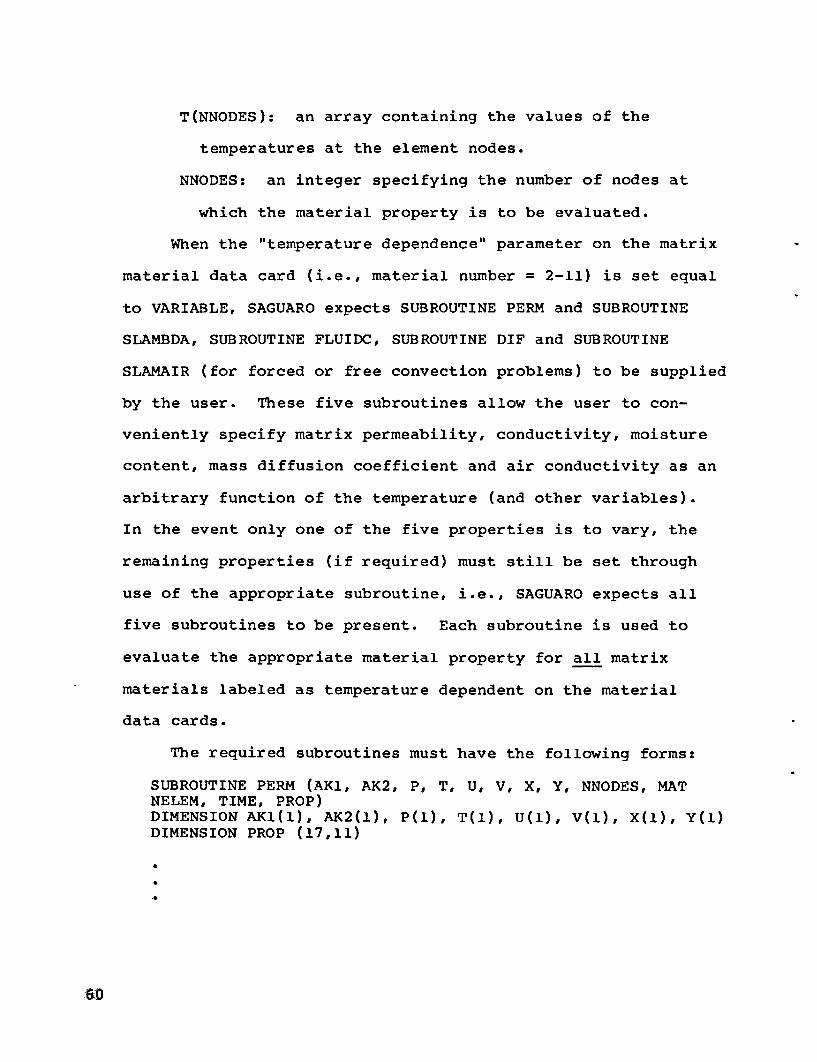
T(NNODES): an array containing the values of the
temperatures at the element nodes.
NNODES: an integer specifying the number of nodes at
which the material property is to be evaluated.
When the "temperature dependence" parameter on the matrix
material data card (i.e., material number = 2-11) is set equal
to VARIABLE, SAGUARO expects SUBROUTINE PERM and SUBROUTINE
SLAMBDA, SUBROUTINE FLUIDC, SUBROUTINE DIF and SUBROUTINE
SLAMAIR (for forced or free convection problems) to be supplied
by the user. These five subroutines allow the user to con-
veniently specify matrix permeability, conductivity, moisture
content, mass diffusion coefficient and air conductivity as an
arbitrary function of the temperature (and other variables).
In the event only one of the five properties is to vary, the
remaining properties (if required) must still be set through
use of the appropriate subroutine, i.e., SAGUARO expects all
five subroutines to be present. Each subroutine is used to
evaluate the appropriate material property for all matrix
materials labeled as temperature dependent on the material
data cards.
The required subroutines must have the following forms:
SUBROUTINE PERM (AK1, AK2, P, T, U, V, X, Y, NNODES, MATNELEM, TIME, PROP)DIMENSION AKl(l), AK2(l), P(i), T(l), U(l), V(l), X(l), Y(1)DIMENSION PROP (17,11)
D6o
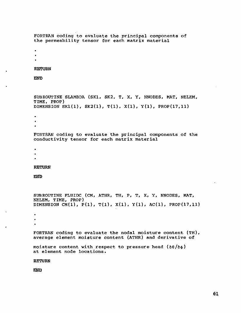
FORTRAN coding to evaluate the principal components ofthe permeability tensor for each matrix material
RETURN
END
SUBROUTINE SLAMBDA (SKl, SK2, T, X, Y, NNODES, MAT, NELEM,TIME, PROP)DIMENSION SKl(l), SK2(l), T(l), X(l), Y(l), PROP(17,11)
FORTRAN coding to evaluate the principal components of theconductivity tensor for each matrix material
RETURN
'END
SUBROUTINE FLUIDC (CM, ATHR, TH, P, T, X, Y, NNODES, MAT,NELEM, TIME, PROP)DIMENSION CM(l), P(l), T(l), X(l), Y(l), AC(l), PROP(17,11)
FORTRAN coding to evaluate the nodal moisture content (TH),average element moisture content (ATHR) and derivative of
moisture content with respect to pressure head (8e/b4 )at element node locations.
RETURN
61
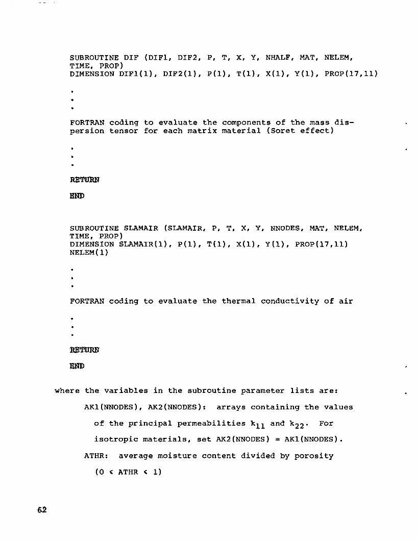
SUBROUTINE DIF (DIF1, DIF2, P, T, X, Y, NHALF, MAT, NELEM,TIME, PROP)DIMENSION DIFl(l), DIF2(1), P(1), T(1), X(l), Y(i), PROP(17,11)
FORTRAN coding to evaluate the components of the mass dis-persion tensor for each matrix material (Soret effect)
RETURN
SUBROUTINE SLAMAIR (SLAMAIR, P, T, X, Y, NNODES, MAT, NELEM,TIME, PROP)DIMENSION SLAMAIR(l), P(1), T(l), X(l), Y(l), PROP(17,11)NELEM(l)
FORTRAN coding to evaluate the thermal conductivity of air
END
where the variables in the subroutine parameter lists are:
AK1(NNODES), AK2(NNODES): arrays containing the values
of the principal permeabilities kll and k2 2 . For
isotropic materials, set AK2(NNODES) = AK1(NNODES).
ATHR: average moisture content divided by porosity
(O 4 ATHR ( 1)
~62
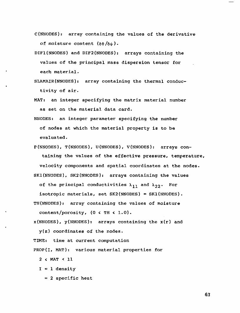
C(NNODES): array containing the values of the derivative
of moisture content (8e/a4 ).
DIFl(NNODES) and DIF2(NNODES): arrays containing the
values of the principal mass dispersion tensor for
each material.
SLAMAIR(NNODES): array containing the thermal conduc-
tivity of air.
MAT: an integer specifying the matrix material number
as set on the material data card.
NNODES: an integer parameter specifying the number
of nodes at which the material property is to be
evaluated.
P(NNODES), T(NNODES), U(NNODES), V(NNODES): arrays con-
taining the values of the effective pressure, temperature,
velocity components and spatial coordinates at the nodes.
SK1(NNODES), SK2(NNODES): arrays containing the values
of the principal conductivities Xll and X2 2. For
isotropic materials, set SK2(NNODES) = SK1(NNODES).
TH(NNODES): array containing the values of moisture
content/porosity, (O 4 TH ( 1.0).
x(NNODES), y(NNODES): arrays containing the x(r) and
y(z) coordinates of the nodes.
TIME: time at current computation
PROP(I, MAT): various material properties for
2 MAT < 11
I = 1 density
= 2 specific heat
63
= 3 thermal conductivity
= 4 I t,
- 6 porosity
= 7 permeability
= 8
for the fluid MAT = 1
I 1 density
= 2 viscosity
= 3 specific heat
= 4 condictivity
= 6 gravitational constant
When the "dispersion" parameter on a matrix material data
card is set to VARIABLE, SAGUARO expects SUBROUTINE DSPERSE to
be supplied by the user. This subroutine must have the follow-
ing formuz
SUBROUTINE DSPERSE (El, E2, E12, U, V, NNODES, MAT)DIMENSION El(l), E2(l), E12(l), U(1), V(l)
FORTRAN coding to evaluate the components of thedispersion tensor for each matrix material
RETURN
MNO
where the variables in the subroutine parameter list are:
El(NNODES), E2(NNODES): arrays containing the values
of the dispersion components. El and E2 contain
the dispersion coefficients taken along the global
-64

coordinate directions; E12 is the off-diagonal
(coupling) component of the dispersion tensor.
U(NNODES), V(NNODES): arrays containing the x and y
velocity components at the nodes.
NNODES: an integer parameter specifying the number of
nodes at which the dispersion coefficients are to be
evaluated.
MAT: an integer specifying the matrix material number
as set on the material data card.
When the volumetric heating parameter, S, on the mate-
rial data card is set equal to VARIABLE, SAGUARO expects
SUBROUTINE SOURCE to be supplied by the user. This subroutine
must have the following form:
SUBROUTINE SOURCE (QVALUE, P. T, X, Y, NNODES, MAT,NELEM, TIME)DIMENSIONS Q VALUE(l), P(l), T(l), X(l), Y(l)
FORTRAN coding to evaluate the volumetric heat sourcefor each material with a variable heat source
RETURN
END
where the variables in the subroutine parameter list are:
QVALUE: the value of the volumetric heating rate.
TIME: the current value of the time.
65

P(NNODES), T(NNODES), X(NNODES), Y(NNODES): arrays
containing the values of the effective pressure, tem-
perature, and spatial coordinates at the nodes.
MAT: an integer specifying the material number as set
on the material data card.
NELEM: element number
NNODES: an integer parameter specifying the number
of nodes at which the material property is to be
evaluated.
The use of a generalized radiation/convection boundary
condition requires that the variation of the heat transfer
coefficient with temperature and/or time be specified. When
the "h" parameter on the SET data card is specified as
VARIABLE, SAGUARO expects SUBROUTINE HTCOEF to be supplied
by the user. The required subroutine has the following form.
SUBROUTINE HTCOEF (HT, TSURF, TREF, XSURF, YSURF, TIME,NELEM, ISET)
FORTRAN coding to evaluate the heat transfer coefficientfor each set number
RETURN
END
where the variables in the subroutine parameter list are:
HT: the heat transfer coefficient.
TSURF: the local surface temperature of the material.
TREF: the reference temperature of the environment as
specified on the set data card.
XSURF, YSURF: the x, y (or r,z) coordinates on the
surface.
TIME: the current value of the time.
NELEM: an integer specifying the element number.
ISET: an integer specifying the "set no." as set on
the BC and SET data cards.
Note that if more than one generalized radiation/convection
boundary condition occurs in a problem, SUBROUTINE HTCOEF is
used for the evaluation of all heat transfer coefficients
that vary with time and/or temperature. The set no. (ISET)
parameter is used to distinguish the different boundary
conditions.
When the boundary condition options PVARY, UVARY, TVARY,
and/or OVARY are employed, SAGUARO expects the appropriate time
history subroutines to be supplied by the user. The corres-
pondence between a particular boundary condition and its
variation with time is established through the "time curve
no." which appears on the BC data card and in the name of the
subroutine providing the time history. The required sub-
routines have the following form:
SUBROUTINE CURVEn (NELEM, PSURF, TSURF, TIME, BCVALUE)
67

FORTRAN coding to evaluate a boundary condition fora specified time history
RETURN
END
where the variables are:
n: an integer specifying the "time curve no." as set
on the BC data card (1 c n < 6).
NELEM: an integer specifying the element number.
PSURF, TSURF: effective pressure and temperature of element.
TIME: the current value of the time.
SETVALUE: the value of the boundary condition for the
current TIME.
The subroutines described above, when required by SAGUARO
should follow the main overlay in the loading sequence. The
control cards necessary to implement user supplied subroutines
are described in a subsequent section.
68

Initial Conditions
The analysis of transient flow problems require the
specification of initial conditions for the dependent var-
iables. For cases where the fluid is initially quiescent and
the temperatures may be assumed uniform (or at least con-
stant over each material), the initial conditions may be set
through a parameter on the material data cards. For problems
where the initial velocity, pressure, and temperature fields
are more complex, SAGUARO accepts initial conditions from an
external storage device (disc or magnetic tape file) denoted
TAPE 19.
In order to be compatible with SAGUARO, the initial con-
ditions must be written to unit 19 with the following un-
formatted FORTRAN write statement:
WRITE (19) TIME, TMAX, TMIN, PMAX, PMIN, NUMEL,
((US (J. I), I = 1, 32), J = 1, NUMEL),
(AMOIST (J), J = 1, NUMEL)
where,
TIME: is the initial time.
TMAX, TMIN: are the maximum and minimum pressures in
the field.
NUMEL: is the number of elements in the mesh (the
present version of SAGUARO requires NUMEL ( 500 and
the Cray version requires NUMEL 4 1000).
US (J, I): is the two-dimensional array containing the
dependent variables (P, T, U, V, 0). The J index
69

indicates the element number; the I index indicates
the degree of freedom number (see page 109).
AMOIST(J): array containing average moisture of
element J. (O < AMOIST 4 porosity)
Note that the I index has an upper limit of 32 which corres-
ponds to the number of degrees of freegom in a quadrilateral
element. If triangular elements are present in the mesh, the
I index must still run to 32; the extra locations in the US
array are ignored by SAGUARO when a triangular element is en-
countered. The ordering of the element degrees of freedom is
given in Appendix B.
When the file containing the initial conditions is
attached to the job, the file name must be TAPE 19. It should
be noted that the output format for SAGUARO is the same as
described above; the output file for SAGUARO is also TAPE 19.
Thus, solutions obtained from SAGUARO may be used directly as
initial conditions for subsequent problems. The use of these
features is demonstrated in the next chapter.
70-

Error Messages
SAGUARO has been supplied with a number of error checks
and tests for bad or inconsistent input data, overflow of
storage, etc. When an error is encountered, an error number
and message is printed and the program is terminated with a
STOP 1 if the error is fatal. The error messages embeded in
SAGUARO, and corresponding explanations are listed below
according to overlay.
(0,O) OVERLAY
DRIVER-UNRECOGNIZED COMMAND -- a command instruction
was expected but was not found or was misspelled.
FFLD-END OF DATA -- an end of file was encountered on
the input file, check termination command.
FFLDSB-INPUT VARIABLE TOO LONG -- an input variable
with more than ten characters was encountered.
RESTART-UNRECOGNIZED COMMAND -- a restart command was
used with an incomplete or misspelled parameter list.
PRINTER-UNRECOGNIZED COMMAND -- an output command was
used with an incomplete or misspelled parameter list.
(1,0) OVERLAY
ELDATA-UNRECOGNIZED COMMAND -- erroneous element,
boundary condition, or looping specification, check
spelling.
ELDATA-LOOP PREVIOUSLY DEFINED -- error in looping
specification, check for third loop within two
existing loops.
71
ELDATA-MAXIMUM NUMBER OF ELEMENTS EXCEEDED -- reduce
number of elements used or re-dimension code.
ELDATA-UNRECOGNIZED DATA ON SET CARD -- a set data card
was used with an incomplete or misspelled parameter
list.
ELDATA-BC APPLIED TO AN UNDEFINED ELEMENT -- a boundary
condition was applied to an element that has not
yet been defined.
ELDATA-EXCESSIVE BOUNDARY CONDITIONS ON ELEMENT -- too
many boundary conditions (i.e., > 6) have been applied
to an element.
ELDATA-UNRECOGNIZED BOUNDARY CONDITION -- boundary con-
dition type is in error, check spelling.
ELDATA-BC ON IMPROPER SIDE OF ELEMENT -- a boundary
condition was specified for an improper side of an
element (1 4 side < 4).
NMESH-IJ MAX OR MIN EXCEEDS SPECIFIED VALUE -- during
generation of the grid points, a part was found with
an imax, jmax, imin, or jmin that exceeded the
specified maxi on the SETUP command.
MATREAD-TOO MANY MATERIALS SPECIFIED -- more than ten
materials were specified.
(2,0) and (10,0) OVERLAY
FORMKFP-BAD ELEMENT JACOBIAN -- a negative element area
was found, check element coordinates and connectivity.
TRI-ZERO JACOBIAN -- a triangular element with a zero
area was found, check element coordinates.
72

QUAD-ZERO JACOBIAN -- a quadrilateral element with a
zero area was found, check element coordinates.
(3,0) OVERLAY
UNZIPP-UNRECOGNIZED COMMAND -- a solution command was
used with an incomplete or misspelled parameter list.
UNZIPP-MAXIMUM STORAGE EXCEEDED -- maximum active storage
exceeded, reduce problem size or re-dimension code.
UNZIPP-COMMAND CARD MISSING -- another solution command
was expected but not found, check for termination
command.
UNZIPP-ZERO PIVOT -- zero on the diagonal of the equation
being eliminated, equation system is singular or element
connectivity is in error.
BCTIME-TIME CURVE NUMBER TOO LARGE -- a time curve number
greater than six was encountered, check data cards and
time history subroutine names.
PRESOLN-INSUFFICIENT STORAGE -- orPREFRNT-INSUFFICIENT STORAGE -- insufficient storage for
element connectivity, reduce problem size or re-
dimension code.
PRESOLN-INSUFFICIENT STORAGE -- orPREFRNT-INSUFFICIENT STORAGE FOR FRONT WIDTH -- reduce
problem size or re-dimension code.
(4,0) OVERLAY
STREAM-INSUFFICIENT STORAGE -- maximum storage for the
stream function field exceeded, reduce problem size
or re-dimension code.
7.3'
(6,0) OVERLAY
PLOTZ-UNRECOGNIZED COMMAND -- a plot command was used
with an incomplete or misspelled parameter list.
CONTOUR-UNRECOGNIZED COMMAND -- error in contour speci-
fication, check spelling on contour type, looping
command, and termination.
TIMEPLT-UNRECOGNIZED COMMAND -- error in history plot
specification, check spelling and termination.
SPLOT-UNRECOGNIZED COMMAND -- error in profile plot
specification, check spelling and termination.
SPLOT-TIMEPLANE DATA CARD NOT FOUND
"M.

Computer Requirements and Control Cards
SAGUARO is a large code (approximately 7500 source state-
ments) that requires a relatively high threshold level of
computer resources in order to operate successfully. SAGUARO
is designed primarily for execution on the CDC 7600/CYBER 76
computer system and the CRAY 1S computer. The following
discussion of computer request parameters and control cards
is specifically directed toward the use of SAGUARO on the
SLA computer system.
The central processor time needed to run SAGUARO is
directly dependent on the number of elements in the mesh and
to a lesser extent on the front width of the problem. To
roughly estimate the CPU time required for a typical job for
isothermal problems, the following formula may be used,
CPU = (Number elements) x (0.03) + (Number elements)
x (Number time steps) x (.02).
For non-isothermal problems, the number of time steps or
iterations should reflect the fact that two equations are
being solved. Note that the constants in the above formula are
accurate for problems of moderate size, but could increase by a
factor of two for very large analyses. Also, the above estimate
of CPU time does not include the time for post-processing the
solution, i.e., computing heat fluxes, plotting, etc.

The amount of Large Core Memory (LCM) needed for a
SAGUARO run is also directly related to the number of elements
in the mesh and the problem front width. Unfortunately, the
LCM required cannot be estimated a priori. The experience
of the user is, thus, the best guide for setting this para-
meter. After completion of a solution, SAGUARO reports the
total LCM required for the job allowing the user to adjust the
requested value for future runs. No LCM request is needed for
SAGUARO (CRAY version).
The SAGUARO program is maintained in an UPDATE form in
the Sandia National Laboratories permanent file (PF) system
and may be accessed by attaching the file with the following
control card:
PFGET, OLDPL, SAGUARO, AU = RREATON. (CDC version)
FILE, OLDPL, RT = 2.
PFGET, OLDPL, CSAG, AU = RREATON. (CRAY version)
Before executing, the file attached with the above control
card must be run through the UPDATE processor and then com-
piled. In the following sections, control card decks are
listed for using SAGUARO in its standard modes of operation.
Run With Plotting:
The control card deck in Figure 6A allows the user to
run SAGUARO and plot results using the RSCORS software package.
The graphical output is post-processed and returned through a
7-6

Versatec plotter at the appropriate Remote Job Entry Terminal
(RJET). Other options for processing and disposing of plotted
output are given in References 8 and 9. To access the CRAY
version of SAGUARO the control stream in Figure 6b should be
executed.
Run With Restart:
Figure 7a shows a control card deck to run SAGUARO (CDC)
and save the solution for later restarting. In this case, the
solution and element data were saved on magnetic tapes; permanent
file storage could also have been used. The listing in Figure 7
is also suitable for restarting a job if the STAGE commands are
modified to cause files TAPE 13 and TAPE 19 to be PRE staged.
The control cards needed to run SAGUARO (Cray) with restarting
are shown in Figure 7b.
Run With Conditions:
The control cards shown in Figure 7a are also suitable for
running a transient analysis with initial conditions provided
from an external source. If the initial conditions are written
on TAPE 19 (in the format discussed previously), then the
listing in Figure 7a is immediately applicable if the request
for TAPE 13 is deleted. The control stream for the Cray ver-
sion of this procedure is shown in Figure 7b.
Run With User Subroutines:
The control cards required to execute SAGUARO (CDC) when
user supplied subroutines are to be included are shown in
7-7
Figure 8a; the equivalent SAGUARO (CRAY) control stream is
shown in Figure 8b.
In Figures 6b, 7b and 8b, the execution of SAGUARO (CRAY)
is carried out through a set of procedure files (SLTLIB10). The
use of these procedures simplifies the access to SAGUARO on
the Cray though, in fact, the basic Cray Job Control Language
can also be used to run the program.
7B

SAGUARO, TXXXX, ECYYY. NAME BOX NO.
USER
PFGET, FLNAME, SAGUARO, AU=RREATON.
UPDATE, P=FLNAME, N, F.
FTN, I=COMPILE, L=O.
PFGET, RSCOR76, AU=SLTHOMP. *
PFGET, RSCDI76, AU=SLTHOMP. *
LIBRARY, RSCOR76, RSCDI76. *
LGO, PL=777777B.
PFGET, POP76, AU=SLTHOMP. *
POP76, TAPE10, POPOUT, HC1. *
COMQ, POPOUT, HC1. *
7-8-9
7-8-9
SAGUARO DATA
6-7-8-9
(1) For large jobs producing large quantities of output,
consideration should be given to using a FICHE, OUTPUT
command to divert the printed output to microfiche.
(2) Graphical output may also be generated via the SCORS soft
ware system by appropriate substitution for the lines
marked by * (see Reference 10). The above control state-
ments assume plots will be generated on a Versatec hard-
copy plotter; other options are available (see Reference 9).
Figure 6a. Control Card Deck (CDC) -- Run With Plotting
79

SAGUARO, TXXXX, STSCZ. NAME BOX NO.
USER .....
S101.
UID. NAME BOX NO.
CUPDATE, P=CSAG, UN=RREATON, F.
CFT, I=COMPILE, L=O.
RSCORLB. *
ASSIGN, DN=POPIN, A=FT10. *
LDR, LIB=RSCORS. *
POP, POPIN, POPOUT, HCl. *
XCOMQ, POPOUT, HC1, CS=R7. *
7-8'-9
7-8-9
SAGUARO DATA
-6-7m--89
(1) For large jobs producing large quantities of output,
consideration should be given to using a XFICHE, $OUT
command to divert the printed output to microfiche.
Figure 6b. Control Card Deck (CRAY) -- Run With Plotting
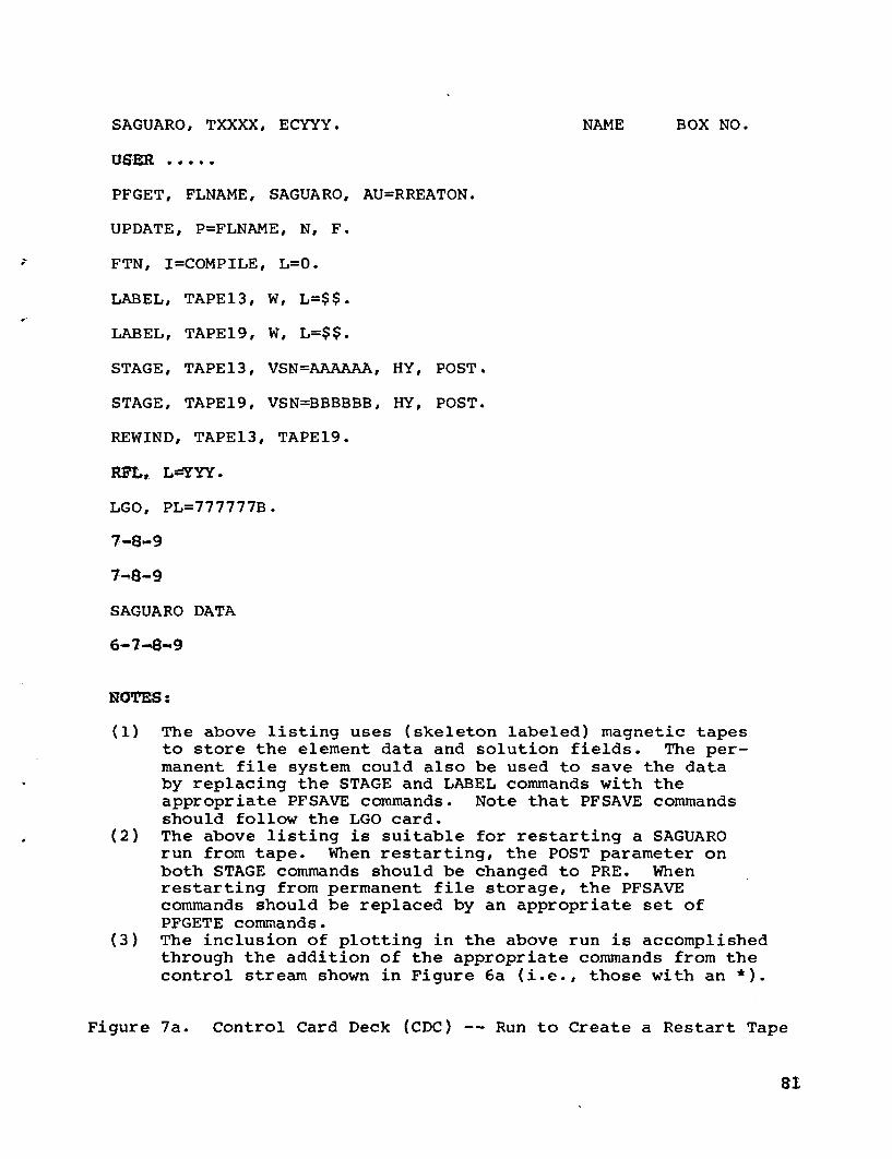
SAGUARO, TXXXX, ECYYY. NAME BOX NO.
USHER .....
PFGET, FLNAME, SAGUARO, AU=RREATON.
UPDATE, P=FLNAME, N, F.
FTN, I=COMPILE, L=O.
LABEL, TAPE13, W, L=$$.
LABEL, TAPEl9, W, L=$$.
STAGE, TAPE13, VSN=AAAAAA, HY, POST.
STAGE, TAPE19, VSN=BBBBBB, HY, POST.
REWIND, TAPE13, TAPE19.
RF'L L=YYY.
LGO, PL=777777B.
7-8-9
7-8-9
SAGUARO DATA
6-7-8-9
NOTES:
(1) The above listing uses (skeleton labeled) magnetic tapesto store the element data and solution fields. The per-manent file system could also be used to save the databy replacing the STAGE and LABEL commands with theappropriate PFSAVE commands. Note that PFSAVE commandsshould follow the LGO card.
(2) The above listing is suitable for restarting a SAGUAROrun from tape. When restarting, the POST parameter onboth STAGE commands should be changed to PRE. Whenrestarting from permanent file storage, the PFSAVEcommands should be replaced by an appropriate set ofPFGETE commands.
(3) The inclusion of plotting in the above run is accomplishedthrough the addition of the appropriate commands from thecontrol stream shown in Figure 6a (i.e., those with an *).
Figure 7a. Control Card Deck (CDC) -- Run to Create a Restart Tape
81

SAGUARO, TXXXX, STSCZ. NAME BOX NO.
USBR 0
=Irz .UID. NAME BOX NO.
CUPDATE, P=CSAG, UN=RREATON, F.
CFT, I=COMPILE,L=O.
LIM.
XTAPEOT, FT13, L=($$), VSN=AAAAAA.
XTAPEOT, FTl9, L=($$), VSN=BBBBBB.
7-8-9
7 -8-9
SAGUARO DATA
6-7-8-9
,MO1z:
(1) The above listing uses (skeleton labeled) magnetic tapesto store the element data and solution fields. The per-manent file system could also be used to save the data byreplacing the XTAPEOT commands with the appropriateXPFSAVE commands.
(2) The above listing is suitable for restarting a SAGUARO runfrom tape. When restarting, the XTAPEOT commands precedethe LDR command. When restarting from permanent filestorage, the XPFSAVE commands are replaced by XPFGETcommands.
(3) The inclusion of plotting in the above run is accomplishedthrough the addition of the appropriate commands from thecontrol stream shown in Figure 6b (i.e., those with an *).
Figure 7b. Control Card Deck (CRAY) -- Run to Create a Restart Tape
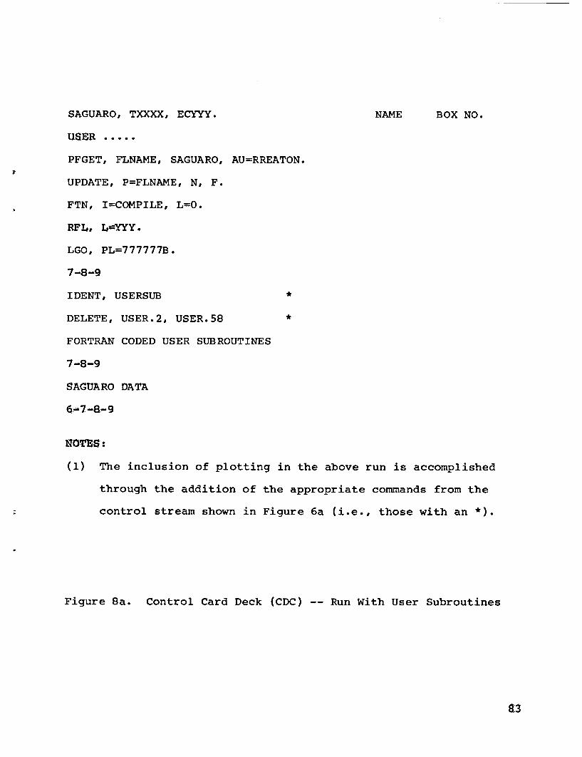
SAGUARO, TXXXX, ECYYY. NAME BOX NO.
USER .
PFGET, FLNAME, SAGUARO, AU=RREATON.
UPDATE, P=FLNAME, N, F.
FTN, I=COMPILE, L=O.
RFL, L=YYY.
LGO, PL=777777B.
7-8-9
IDENT, USERSUB *
DELETE, USER.2, USER.58 *
FORTRAN CODED USER SUBROUTINES
7-8-9
SAGUARO DATA
6-7-8-9
SOWS:
(1) The inclusion of plotting in the above run is accomplished
through the addition of the appropriate commands from the
control stream shown in Figure 6a (i.e., those with an *).
Figure 8a. Control Card Deck (CDC) -- Run With User Subroutines
83

SAGUARO, TXXXX, STSCZ. NAME BOX NO.
USER .
S=LIB.
UID. NAME BOX NO.
CUPDATE, P=CSAG, UN=RREATON, F.
CFT, I=COMPILE, L=0.
7 -B-9
IDENT, USERSUB *
DELETE, USER.2, USER.58 *
FORTRAN CODED USER SUBROUTINES
7-8'8-9
SAGUARO DATA
-6-7-8-9
Ro:
(1) The inclusion of plotting in the above run is accomplished
through the addition of the appropriate commands from the
control stream shown in Figure 6b (i.e., those with an *).
Figure 8b. Control Card Deck (CRAY) -- Run With User Subroutines

A NOTE TO EXPERIENCED MARIAH USERS
The following discussion should be helpful to potential
SAGUARO code users who have already "mastered" the operating
features of MARIAH. SAGUARO is set up to accept data decks
for transient problems which have been designed for MARIAH.
When the UNSAT material input data cards or user subroutines,
page 15, are not supplied, the following default values are
used (see Equation (10))
Dll D 2 2 =D C xair 0
and SAT = 1.0.
Thus, the general equation for unsaturated flow (Equation (10))
reduces to Equation (11). Consequently, under these conditions,
the equations solved in SAGUARO and MARIAH are identical.
If the material card for a specific material sets
temperature dependence to VARIABLE, then Diji C, Xair and SAT
in addition to Xi. and ki. must be defined through five user
subroutines and the UNSAT card for that material may be omitted.
This would be the most realistic mode for partially saturated
flow analysis where the coefficients in Equation (11) would be
highly nonlinear.
85

SAMPLE CALCULATION
A sample problem has been included in this section to
demonstrate the use of the previously described command cards
and some of the capabilities of the SAGUARO code. Though this
example illustrates many of the salient features of the code,
all possible combinations of capabilities could not be covered.
Further understanding of code usage can be obtained from the
examples given in the MARIAH manual.4
The sample problem involves the one-dimensional infiltra-
tion of rain and heat into hard rock consisting of several
strata which is partially saturated at time zero, see Figure 9.
- Ground Surface. ' - Initial Conditions
. . Partially- . * . . Saturated
.~~~~~~~~~~ ly, . . ~~~~~~~Fullyj.ji} ' ,.Saturated
. e *. . I' * t
FIGURE 9. Geometry Used in SampleInfiltration Problem
86
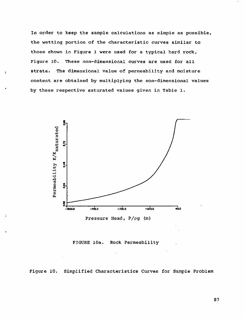
In order to keep the sample calculations as simple as possible,
the wetting portion of the characteristic curves similar to
those shown in Figure 1 were used for a typical hard rock,
Figure 10. These non-dimensional curves are used for all
strata. The dimensional value of permeability and moisture
content are obtained by multiplying the non-dimensional values
by these respective saturated values given in Table 1.
>1v43 0.6-I
15000 -1115.0 -7X.0 -X5D 40.0
Pressure Head, P/pg (m)
FIGURE 10a. Rock Permeability
Figure 10. Simplified Characteristics Curves for Sample Problem
87
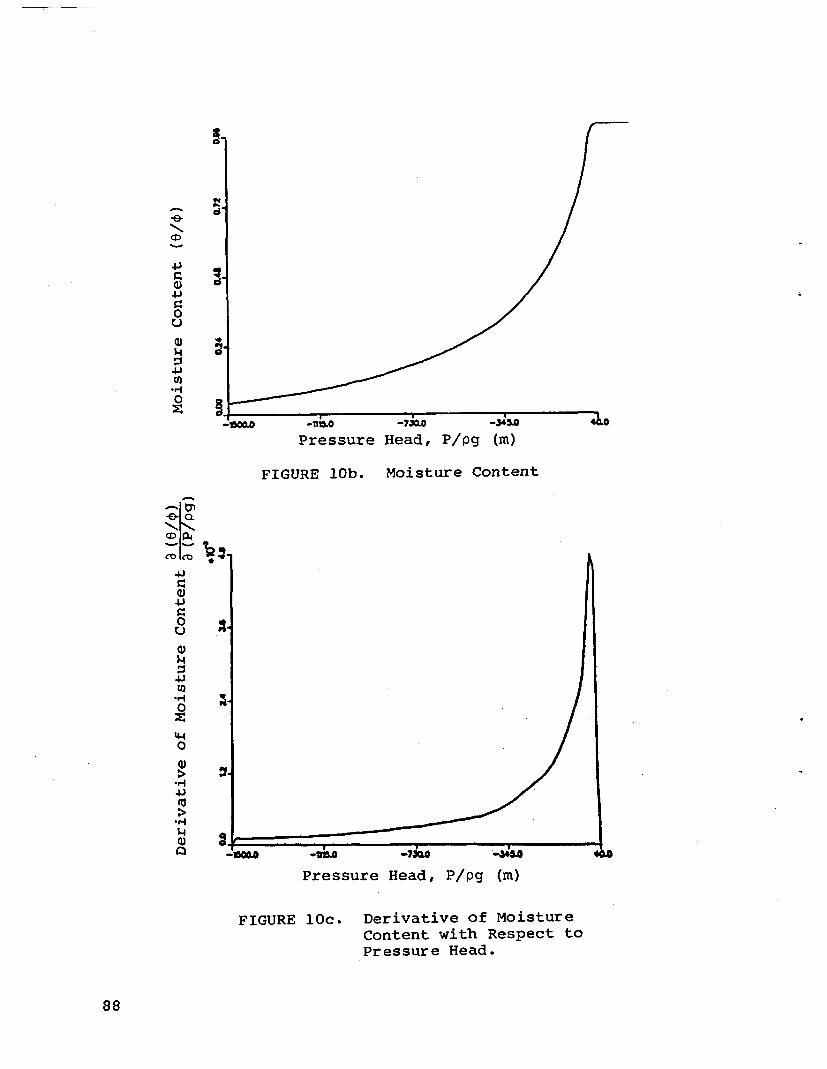
-6-
41.)
.1-)
0U
U)
4-IU)
*r107z
Pressure Head, P/pg (m)
FIGURE lOb. Moisture Content
-IO.
a) 0
4J
U)'4j
U)
0
4.)
'440)
Pressure Head, P/pg (m)
FIGURE lOc. Derivative of MoistureContent with Respect toPressure Head.
88
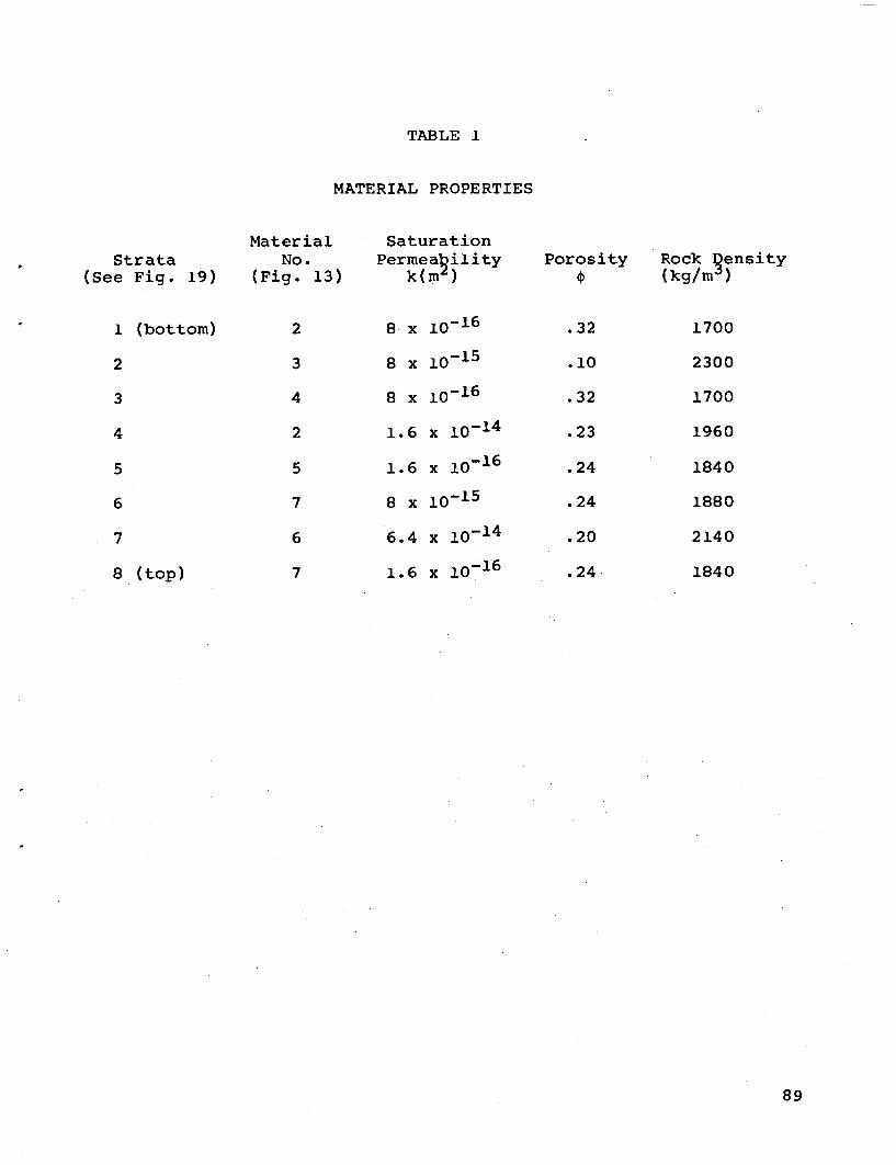
TABLE 1
MATERIAL PROPERTIES
Strata(See Fig. 19)
MaterialNo.
(Fig. 13)
SaturationPermeauility
k( )Porosity Rock ensity
(kg/rn )
1 (bottom)
2
3
4
5
6
7
8 (top)
2
3
4
2
5
7
6
7
8 x l0-16
8 x 10 15
8 x 10-16
1.6 x 10⁻¹⁴
1.6 x 10 16
8 x 10-15
6.4 x i0-14
1.6 x 10 16
.32
.10
.32
.23
.24
.24
.20
.24
1700
2300
1700
1960
1840
1880
2140
1840
89

The boundary conditions for the test case are:
1. Rain is such that it feeds the soil at a rate of 1.0
m/yr.
2. Linear initial pressure head (4i) t = 0 (fluid velocity
is zero everywhere).
3. No flow through bottom boundary.
90
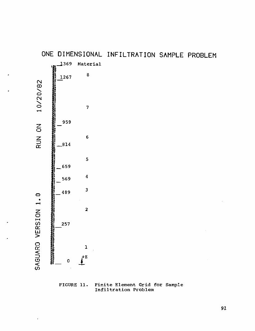
aNoc'Nc(NNc-4
z
0
z0
C)
Vo
w0
U)
co
U)
ONE DIMENSIONAL INFILTRATION SAMPLE PROBLEMl1369 Material
) 1267 8
* 7
2 959
> 2 _814
5
9 _ 659
X_ 569 4
3-
A_489 3
2 84 2
.
_257
1 ~~~1
° 4Z
FIGURE 11. Finite Element Grid for SampleInfiltration Problem
91

13691
0 -620 +750
Pressure Head (2), mPg
FIGURE 12: Initial Pressure Head
The computational mesh for this problem consisted of one-
hundred elements, Figure 11, and the initial pressure
distribution is shown in Figure 12. A listing of the input
data and control cards is given in Figure 13. The units
chosen for this problem are kg, m and seconds. The required
users subroutines are listed in Figure 14.. Figure 15 shows
the output that can be expected from 'the input described above.
92

* ONE DIMENSIONAL INFILTRATION SAMPLE PROBLEMSETUP. 1 , 3 . , PLOTWATER . 1 . 994. ,7.8E-04 . 4190. . 0.60. 0.0 . +9.8 . . 35.STARTA1,2,1840.,1600..2.5,.. 24.1.6E-16 ... .VARIABLE. 35..7.301E6STRATA2,3,2140.,1600.,2.5 ... 20.6.4E-14....VARIABLE,,35.,7.301E6STARTA34.41880..1600.,2.5,...24.8.OE-15, ,,VARIABLE,.35..7.301E6STRATA5,5,1960.,1600.,2.5,,,. 23.1.6E-14... VARIABLE,.35.,7.301E6STRATA6.6,2300.,1600.,2.5,.,. 10,8. OE-15., a.VARIABLE,, 35.,7. 301E6TOP .7.1700.,1600..2 5.5,.32.8.OE-16. ,.VARIABLE,,35.,7.301E6END1. 1.3.390. 10. 10.00,0.257,2571,39,3.730. 10. 10.0257,257.489,4891.73.3.850. 10, 10.0489,489.569,5691,85.3,970.10.10. 0569.569,659.6591,97.3.1210. 10, 10. 0659.659.814,8141.121,3.1410. 10. 10.0814,814, 959. 9591,141.3,1850, 10, 10.0959.959.1267.12671,185.3.2010, 10, 10. 01267,1267.1369.1369ENDJLOOP.19.2QUAD8/4,2.1.1JENDJLOOP.17.2QUAD8/4,3,1,39JENDJLOOP.6.2GUAD8/4*4,1.73JEND
$ REG 1
$ REG 2
$ REG 3
* REG 4
$ REG 5
$ REG 6
$ REG 7
$ REG 8
$ REQ 1
$ REG 2
$ REG 3
FIGURE 13a. Input Data
Figure 13. Code Requirements for Sample Problem
93
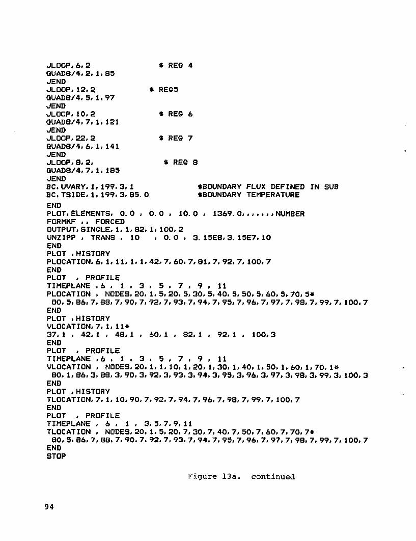
JLOOP.6t2 $ REG 4OUAD8/4. 2. 1. 65JENDJLOOP.12.2 $ REG5OUAD8/4.5.1.97JENDJLOOP.10.2 $ REG 6OUADB/4.7,1.121JENDJLOOP.22.2 $ REG 7OUADS/4.s.1.141JENDJLOOP.6.2. $ REQ 8QUAD8/4.7,1. 185JENDBC.UVARY.1.199.3,1 $BOUNDARY FLUX DEFINED IN SUBBCTSIDE.1.199.3,B5.0 $BOUNDARY TEMPERATURE
ENDPLOT.ELEMENTS. 0.0 . 0.0 . 10.0 * 1369.0.......NUMBERFORMKF .. FORCEDOUTPUT.SINGLE.1.1.682,1.100,2UNZIPP . TRANS . 10 * 0.0 . 3.15E8.3.15E7.10ENDPLOT .HISTORYPLOCATION.6.1.11.1.1.42.7.60.7.81.7.92.7.100.7ENDPLOT . PROFILETIMEPLANE .6 , 1 . 3 . 5 . 7 . 9 . 11PLOCATION . NODES,20.1.5.20.5.30.5.40.5.50.5. 60.5. 70.5*60,5,86,7.88.7.90.7,92.7.93.7.94,7.95.7,96.7.97,7,98,7.99.7.100.7
ENDPLOT .HISTORYVLOCATION.7.1,11*37,1 . 42,1 , 48.1 , 60.1 . 82.1 . 92.1 . 100.3ENDPLOT . PROFILETIMEPLANE .6 . 1 . 3 . 5 . 7 . 9 . 11VLOCATION . NODES,20,1,1,10,1,20.1,30,1,40.1,50,1,60.1,70,1*80. 1.86. 3,.88. 3. 90, 3, 92.3. 93. 3. 94. 3, 95. 3. 96. 3. 97, 3, 98. 3. 99. 3. 100. 3
ENDPLOT .HISTORYTLOCATION.7.1.10.90.7.92.7.94,7.96,7.98,7.99.7.100. 7ENDPLOT . PROFILETIMEPLANE . 6 . 1 . 3,5.7.9,11TLOCATION . NODES.20,1.5.20.7.30. 7,40.7.50.7.60.7.70,7*80,5.86.7.88,7.90.7.92.7.93.7,94,7,95.7.96.7,97.7.98.7.99.7.100.7
ENDSTOP
Figure 13a. continued
94

SYUCONE.T70,EC350.USER(RREATON.CHARGE.1286424)PFOET.OLDPL.SAGUARO.UPDATEF.FTN.I=CGMPILE.L=O.PMD.REWINDTAPE12,TAPE19.RFLL=350.MAP.PART.PFGETVTSCORS.AU=PLOTLIB.ATTACHFXMATHAU=MATHLIB.LIBRARYFXMATH.VTSCORS.LDSET(PRESET=NGINF)LGO.PFREPL.TAPE12. YODM.CT=PU.PFREPLTAPE19. PTOMCT=PU.REWINDTAPE10.LIERARY.COMLIB.COMG.TAPElO.HC1.REWIND, OUTPUT.COPY. OUTPUT. DUMMY.FICHE, DUMMY.
Figure 13b. CDC 7600 Control Cards
CSAG T60 STSCZ.
USER(RREATON,(NOS PASUORD))SLTLIB.UID. RR EATON BOX 1134CUPDATEPuCSAG2,UN-RREATONF.CFT(I-COMPILEON-Z,Le0)RSCORLB.ASSIGNDN-POPIN, AFTI0.ACCESSDN-FXMATH,ID-MATHCRA.LDRLIB-RSCORStFXMATH.POPPOPINPOPOUT,HCI.XCOMQPOPOUTHC1,CS-R7.REUINDDN-SOUT.COPYD,I*SOUT,O-FOUT.XFICHEFOUT,T*'SAGUARO'.EXIT.DUMPJOB.DEBUG.REUINDoDN-SOUT.COPYDI-SOUT,OuFOUT.XFICHE,FOUT,T-'SAGUARO'.
Figure 13c. CRAY Control Cards with Updating Done on CDC 6600
95

SUBROUTINE FLUIDC(CM.ATHRPHIT.YX,,KURELMATNELEMTIMEPROP)CC THIS SUB CALC THE MOISTURE CONTENT AND DER OF MOISTURE CONTENT WRT PH(1/MC UNITS - KGMSEC.C
DIMENSION CM(8),TH(8),PHI(B).PH(B),T(B),X(l),Y(l),PROP(17,7)DIMENSION PHD(20),WDAT(20),YP(20),YPP(20),W(60),YPIC1),YPPIC1)DATA RHOG/9.714E3/DATA(PHD(I),Iin 15)/-1500.0,-500.,-270.,-200..-90..-50.
le -40.,-30. .-20.,-10.,.0.0,10.,20..30..40. /DATA(WDAT(I).Ii, 15)/0.04,0.256,0.398,0. 470.0.6351.. 725,. 751,. 789. B15,. 855P. 905,.961,. 985,. 997a 1./DATA IFIRST/1/.W(1)/-1./ , EPS/-1./IMAX-15IF(IFIRST.EG.1)1 CALL SPLIFT(PHD.WDAT.YPYPP.IMAX,W IERR,0,0,0,0,0)IFIRST-2DO 20 %J-1.KURELPH(J)=PHI(J)/RHOG - Y(J)IF(PH(J).GE.PHD(IMAX)) TH(J)-WDAT(IMAX)IF(PH(J).GE. PHD(IMAX)) CM(J)=O.OIF(PH(J).GE.PHD(1) AND. PH(J) .LT. PHD(IMAX))1 CALL SPLINT(PHDWDATYPPIMAX.PH(J).TH(J),CM(J)sYPPI.1,KERR)IF(PH(J) .LE. PHD(1)) TH(J)=WDAT(1)IF(PH(J) .LE. PHD(1)) CM(J)-O.OCM(J) - CM(J)*PROP(6,MAT)
;.0 CONTINUEATHR=-.25*(TH(1)+TH(2)+TH(3)+TH(4))1 +0.5*(TH(5)+TH(6)+TH(7)+TH(B))
C GIVES THETA/THETA MAXRETURNEND
Figure 14a. Moisture Content and Derivative of Moisture Content
SUBROUTINE DIF(DIF1.DIF2,P,.TXY. NHALF.MAT.NELEM.TIME,PROP)CC DIFUSION COEFICIENT FOR MASS TRANSPORTC
DIMENSION DIF1(4),DIF2(4),P(B),PH(6),T(8),X(8),Y(8)DIMENSION PROP(17,7)DO 10 J-1,NHALFDIF2(J)=1.E-8DIF1(J)=1.E-8
10 CONTINUERETURNEND
Figure 14b.) Coefficient for Mass Transport (D1l and D2 2)
Figure 14. User Subroutines for the One-DimensionalInfiltration Problem
96

SUBROUTINE PERM(CONDI.COND2.PHI.TUV.VX. YNHALF.MATNELEM.TIME1.PROP)
CC CALCULATES PERMEABILITY (M**2)C UNITS - KG.M.SEC.C
DIMENSION COND1(1).COND2(1).PHI(8).PH(6).T(8).Y(1)DIMENSION PROP(17.7)DIMENSION PHD(20).HKD(20).YP(20).YPP(20).W(60).YPI(1).YPPI(1)DATA RHOQ/9.714E3/DATA(PHD(I).1=1.15)/-1500.0.-500.,-270. -200..-90. -50.
1. -40. 1-30. .- 20. ,-10. 10.0, 10. .20. .30. .40./DATA(HKD(I).1=1.15)/0.04.0.256.0.398,0.470,0.6351.. 725,. 751.. 78. .815. 655.. 905.. 961.. 965.. 997. 1./DATA IFIRST/1/.W(1)/-1./ . EPS/-1./IMAX=15IF(IFIRST.EG.1)
1 CALL SPLIFT(PHD.HKD.YP.YPP.IMAXW.IERR.0.0,0.0.0)IFIRST=2DO 20 J=1.NHALFPH(J)=PHI(J)/RHOG - Y(J)IF(PH(J).GE.PHD(I)1AX)) COND1(J)=HKD(IMAX)IF(PH(J).GE.PHD(1) .AND. PH(J) .LT. PHD(IMAX))
1 CALL SPLINT(PHD.HKD.YPP.IMAX.PH(J).CONDI(J).YPI.YPPI.1.KERR)IF(PH(J) .LE. PHD(1)) CONDI(J)=HKD(1)CONDI(J) = COND1(J)*PROP(7,MAT)COND2(J) = COND1(J)
20 CONTINUERETURNENDSUBROUTINE SLAMBDA (SKI.SK2,T.X.V.NNODES.MAT.NELEM.TIME)DIMENSION SK1(1) . SK2(1) . Tt1)DO 10 I=1.NNODESSK2(I) = 10.0SK1() = 10.0
10 CONTINUERETURNENDSUBROUTINE CURVE1 (NELEM.PSURF.TSURFTIME.VALUE)VALUE=3.17E-8RETURNEND
Figure 14c. Permeability
97

SUBROUTINE SLAMBDA (SK1.SK2.T X. YNNODESMAT.NELEM,TIME)DIMENSION SK11) . SK2(1) , T(1)DO 10 I=1.NNODESSK2(I) = 10.0SKICI) = 10.0
10 CONTINUERETURNEND
Figure 14d. Thermal Conductivity
SUBROUTINE CURVEI (NELEM.PSURF.-TSURFPTIME1 VALUE)VALUE=3.17E-8RETURNEND
Figure 14e. Curve for Water Source
98

+,,ONE DIMENSIONAL INFILTRATION SAMPLE PROBLEM1.*40613110 __
1.2660116i
w 6
U,
IJJ
0L
*6I6.06 661 16
*61..S0866186
* I .66606I116 2.66686116 ' 3.6*SSSII - 4.6666 X+16
T I ME
Figure 15a. Effective Pressure as a Function of Time for Z =0, 569, 814, 1113, 1267, and 1369 m.
Figure 15. Graphics Output from Sample Infiltration Problem
99

,,ONE DIMENSIONAL INFILTRATION SAMPLE PROBLEM1.4 6i1.1
I -I I I
iIIIl.2SSSSXIl
Ir 1. 60 ISSNI
w
a-
*56
S. SsS3SZIS01
0 200 400 600D I STANCE
800 1000 1200 1400
Figure 15b. Effective Pressure as a Function of Depth forTime = 0, 2, 4, 6, 8, and 10 yr.
100
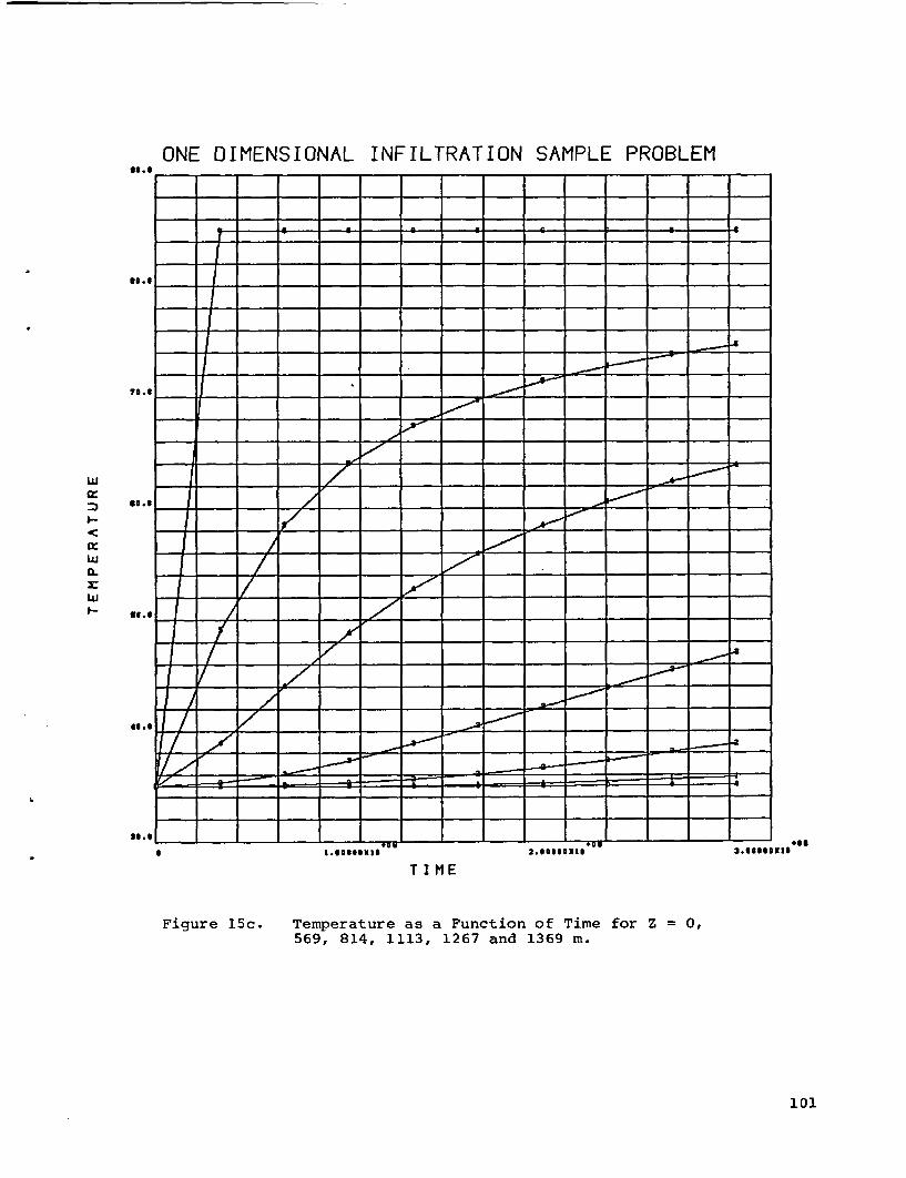
ONE DIMENSIONAL INFILTRATION SAMPLE PROBLEMS...
....
1...
f~- ==-*-_I__ ====_ ___I ___-
0:
CL
7 /....-- . - l1 4 4-~- -- - -+- -_ , t -
I W/
so..
t~~- _4 , - - - = == -
i _S __ _ Z _~~~~~-A_-_-_
1 -__4
4..6
2...- ...
S 1.60S09116 2.6666o11l 3.60666 X1
T I ME
Figure 15c. Temperature as a Function of Time for Z = 0,569, 814, 1113, 1267 and 1369 m.
101

ONE DIMENSIONAL INFILTRATION SAMPLE PROBLEM33.3
w
I--
a-
I.- so
_.3 __________
_. __________
_.3 _________
.. ; i~ i; f --.---- -=4ig
..
4.
3.
200 400 600 800 1000 1200 1400
DISTANCE
Figure 15d. Temperature as a Function of Depthat Time = 0, 2, 4, 6, 8, and 10 yr.
102

ONE DIMENSIONAL INFILTRATION SAMPLE PROBLEM-3,2. 6368 SI I
-2.64ggSi.t t
-4.34*8S*S2I3
-1 M -to
-6.."..sxt.-1
I--
-4LU
4
a-.
LU
-..-I.Sggs.RI
-1.200SX913-am
a I .eon0Xze 2.TI 61ME
T IM E
.
3. 6 50818 4.90009213
Figure l5e. Velocity as a Function of Time for Z = O.569, 814, 1113, 1267 and 1369 m.
103

,, ONE DIMENSIONAL INFILTRATION SAMPLE PROBLEMI.Sellexis
fI-
-.4
0
LU -2.91080XIS 4
C-)
LU
I..0 ~ ~ -S
-3. S 46ests-8
a~~~~~~~~~~~~~~~~~~~~~~~~
.&UU 400 600 8UU 1000 1200 1400
DISTANCE
Figure 15f. Velocity as a Function of Depth atTime = 0, 2, 4, 6, 8 and 10 yr.
104

ONE DIMENSIONAL INFILTRATION SAMPLE PROBLEM1.6.
I--U)
0
...3. 66 66x2
T I ME
Figure 15g. Moisture Content as a Function of Time forZ = 0, 569, 814, 1113, 1267 and 1369 m.
105
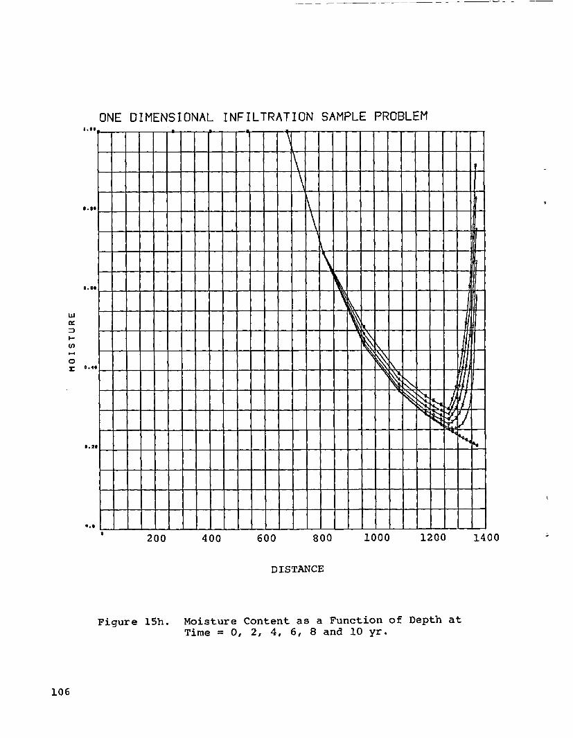
1.01
I. e
I.1
w
0
ONE DIMENSIONAL INFILTRATION SAMPLE PROBLEM
___ _ _ A___ _ _3___ ___ ___
pt00 ____
I ____ ____ ~ ~ ~ ~
* .2
e. I0
200 400 600 800 1000 1200 1400
DISTANCE
Figure 15h. Moisture Content as a Function of Depth atTime = 0, 2, 4, 6, 8 and 10 yr.
106
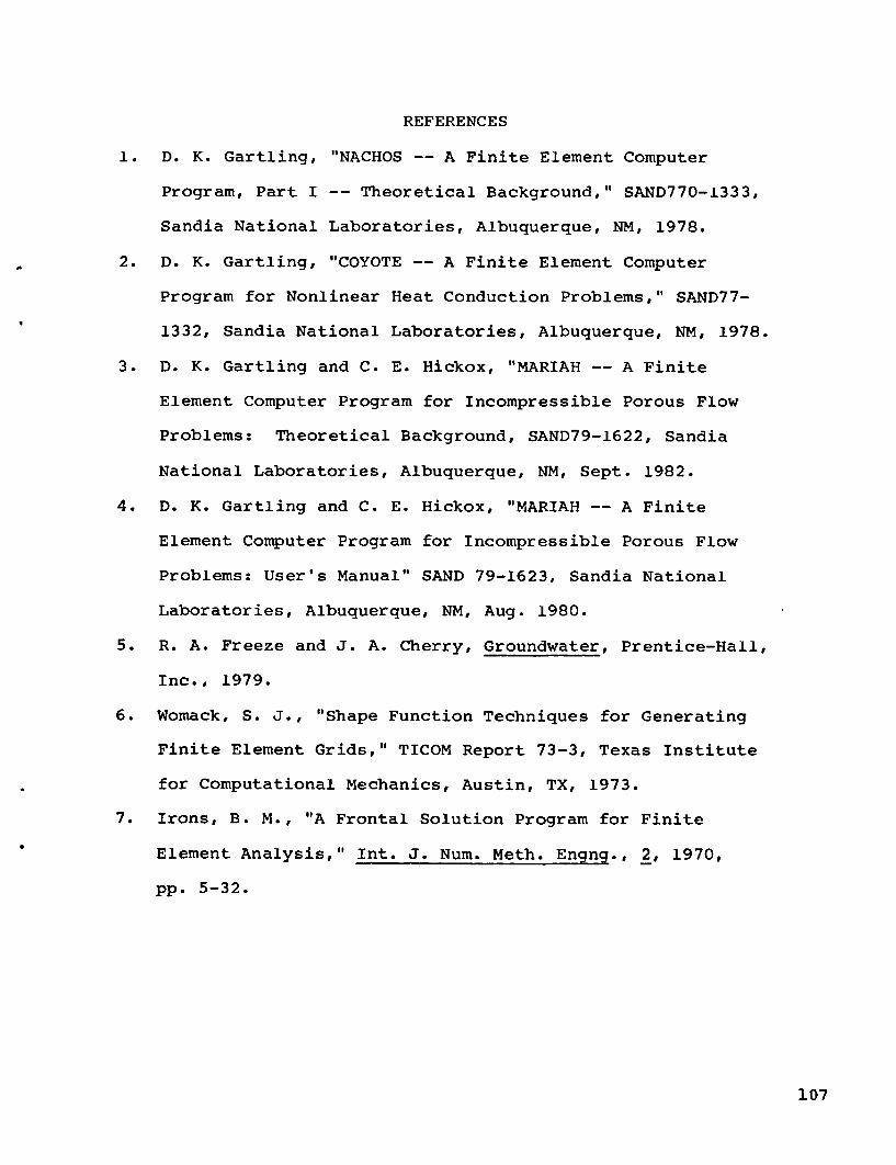
REFERENCES
1. D. K. Gartling, "NACHOS -- A Finite Element Computer
Program, Part I -- Theoretical Background," SAND770-1333,
Sandia National Laboratories, Albuquerque, NM, 1978.
2. D. K. Gartling, "COYOTE -- A Finite Element Computer
Program for Nonlinear Heat Conduction Problems," SAND77-
1332, Sandia National Laboratories, Albuquerque, NM, 1978.
3. D. K. Gartling and C. E. Hickox, "MARIAH -- A Finite
Element Computer Program for Incompressible Porous Flow
Problems: Theoretical Background, SAND79-1622, Sandia
National Laboratories, Albuquerque, NM, Sept. 1982.
4. D. K. Gartling and C. E. Hickox, "MARIAH -- A Finite
Element Computer Program for Incompressible Porous Flow
Problems: User's Manual" SAND 79-1623, Sandia National
Laboratories, Albuquerque, NM, Aug. 1980.
5. R. A. Freeze and J. A. Cherry, Groundwater, Prentice-Hall,
Inc., 1979.
6. Womack, S. J., "Shape Function Techniques for Generating
Finite Element Grids," TICOM Report 73-3, Texas Institute
for Computational Mechanics, Austin, TX, 1973.
7. Irons, B. M., "A Frontal Solution Program for Finite
Element Analysis," Int. J. Num. Meth. Engng., 2, 1970,
pp. 5-32.
107

APPENDIX A
CONSISTENT UNITS
The following list provides examples of consistent units for
quantities encountered in the use of the MARIAH program:
Quantity
Length
Time
Mass
Force
Energy
Temperature
GravitationalAcceleration
Density
Velocity
Stress (Pressure)
Viscosity
Specific Heat
Power
Heat Flux
Heat TransferCbefficient
Thermal Conductivity
Thermal Dispersion
IntrinsicPermeability
English
foot (ft)
second (s)
lbm
lbft/ss
Btu
Fahrenheit (F)or Rankine (R)
ft/s 2
lb ft3
ft/s
lbr/ ft-s 2
l1b/ft-s
Btu/l v-F
Btu/s
Btu/ft2 -s
Btu/ft 2 -s-F
Btu/ft2 -s-F
Btu/ft-s-F
ft 2
Metric
centimeter (cm)
second (s)
gram (g)
g-cm/s 2
calorie (cal)
centigrade (C)or Kelvin (K)
cm/s2
g/cm3
cm/s
g/cm-s 2
g/CM-s
cal/g-C
cal/s
cal/cm2 -s
cal/cm2 -s-C
cal/cm-s-C
cal/cm-s-C
CM2
SI
meter (m)
second (s)
kilogram (kg)
Newton (N)
Joule (J)
Kelvin (K)
M/s 2
kg/m3
m/s
pascal (N/m 2)
pascal-s
JAg-K
J/s (Wtt)
J/m2 -s
jln~-s-K
J/mr-s-K
m2
108

Quantity
Porosity
Coefficient ofVolume Expansion
Volume HeatSource
English
___
1/F
Btu/ft3-s
Metric
___
1/C
cal/cm3-s
Si
_ _
1/K
J/m 3 -s
Ca
lb -ft32.174 inmf
lbf-s 2
4.755 x 10⁻¹³
BTU
S-ft 2 _R 4
n.d.
ft/s *R
1 g-cm
dyne-s2
1.355 x 10⁻¹²
cal
s-cM2 -K 4
n.d.
cM 2 /s -K
1 kg-m
N-s
5.6697 x 10⁻⁸
Js5m2_K4
n.d.
M2 / s *- K
9
109

APPENDIX B
DEGREE OF FREEDOM NUMBERING
The following list provides the correspondence between the
nodal point variables in an element and the degree of freedom
numbering scheme used internally in MARIAH. The node numbers
shown below refer to Figure 5.
Quadrilateral Element:
Node No. Variable Degree of Freedom Number1 P 1
T 9U 17V 21e 25
2 P 2T 10U 18V 22e 26
3 P 3T 11U 19V 236 27
4 P 4T 12U 20V 243 28
5 P 5T 130 29
6 P 4T 14e 30
7 P 7T 15o 31
8 P 8T 160 32
110

Triangular Element:
Node No. Variable Degree of Freedom Number
1 pTUVe
19
172125
2 pTUV
pTUV
210182226
311192327
3
4 pT6
41228
5 pTe
51329
6 pT
61430
111

Distribution;Unlimited ReleaseUC-70
J. W. Bennett, DirectorGeologic Repository DivisionU.S. Department of EnergyNE-22Washington, DC 20545
M. W. FreiGeologic Repository DivisionU.S. Department of EnergyNE-22Washington, DC 20545
C. R. CooleyGeologic Repository DivisionU.S. Department of EnergyNE-22Washington, DC 20545
C. H. GeorgeGeologic Repository DivisionU.S. Department of EnergyNE-22Washington, DC 20545
J. J. FioreGeologic Repository DivisionU.S. Department of EnergyNE-22Washington, DC 20545
J. G. VlahakisGeologic Repository DivisionU.S. Department of EnergyNE-22Washington, DC 20545
T. P. LongoGeologic Repository DivisionU.S. Department of EnergyNE-22Washington, DC 20545
C. KlingsbergGeologic Repository DivisionN.S. Department of EnergyNE-22Washington, DC 20545
NTS Project ManagerHigh-Level Waste Technical
Development BranchDivision of Waste ManagementU.S. Nuclear Regulatory CommissionWashington, DC 20555
Chief, High-Level Waste TechnicalDevelopment Branch
Division of Waste ManagementU.S Regulatory CommissionWashington, DC 20555
J. 0. Neff, Program ManagerNational Waste Terminal
Storage Program OfficeU.S. Department of Energy505 King AvenueColumbus, OH 43201
N. E. CarterBattelleOffice of Nuclear Waste Isolation505 King AvenueColumbus, OH 43201
ONWI Library (5)BattelleOffice of Nuclear Waste Isolation505 King AvenueColumbus, OH 43201
0. L. Olson, Project ManagerBasalt Waste Isolation Project OfficeU.S. Department of EnergyRichland Operations OfficePost Office Box 550Richland, WA 99352
R. DejuRockwell International Atomics
International DivisionRockwell Hanford OperationsRichland, WA 99352
112
Distribution (cont.):
Governor's Office PlanningCoordinator
Nevada State Planning CoordinationState Capitol Complex, Second FloorCarson City, NV 89710
J. I. Barnes, DirectorDepartment of EnergyState of Nevada400 W. King St., Suite 106Carson City, NV 89710
K. Street, Jr.Lawrence Livermore National
LaboratoryMail Stop L-209P.O. Box 808Livermore, CA 94550
L. D. RamspottTechnical Project OfficeLawrence Livermore National
LaboratoryP.O. Box 808Mail Stop L-204Livermore, CA 94550
D. C. HoffmanLos Alamos National LaboratoryP.O. Box 1663Mail Stop E-515Los Alamos, NM 87545
D. T. OakleyTechnical Project OfficerLos Alamos National LaboratoryP.O. Box 1663Mail Stop F-671Los Alamos, NM 87545
W. W. Dudley, Jr.Technical Project OfficerU.S. Geological SurveyP.O. Box 25046Mail Stop 418Federal CenterDenver, CO 80225
R. W. LynchTechnical Project OfficerSandia National LaboratoriesP.O. Box 5800Organization 9760Albuquerque, NM 87185
G. F. RudolfoTechnical Project OfficerSandia National LaboratoriesP.O. Box 5800Organization 7254Albuquerque, NM 87185
A. E. StephensonSandia National LaboratoriesP.O. Box 14100Organization 9764Las Vegas, NV 89114
D. L. Vieth, Director (5)Waste Management Project OfficeU.S. Department of EnergyP.O. Box 14100Las Vegas, NV 89114
D. F. Miller, DirectorOffice of Public AffairsU.S. Department of EnergyP.O. Box 14100Las Vegas, NV 89114
D. A. Nowack (8)U.S. Department of EnergyP.O. Box 14100Las Vegas, NV 89114
B. W. Church, DirectorHealth Physics DivisionU.S. Department of EnergyP.O. Box 14100Las Vegas, NV 89114
A. E. GurrolaHolmes & Narver, Inc.P.O. Box 14340Las Vegas, NV 89114
W. S. Twenhofel820 Estes StreetLakewood, CO 80215
113
Distribution (cont.):
H. D. CunninghamReynolds Electrical &
Engineering Company,P.O. Box 14400Mail Stop 555Las Vegas, NV 89114
Inc.
J. A. CrossFenix & Scisson, Inc.P.O. Box 15408Las Vegas, NV 89114
R. H. MarksU.S. Department of EnergyCP-1, M/S 210P.O. Box 14100Las Vegas, NV 89114
A. R. Hakl, Site ManagerWestinghouse - AESDP.O. Box 708Mail Stop 703Mercury, NV 89023
M. SpaethScience Applications, Inc.2769 South Highland DriveLas Vegas, NV 89109
G. TomsicUtah Dept. of Community
Economic DevelopmentRoom 6290, State Office Bldg.Salt Lake City, UT 89114
U.S. Department of Energy (2)Technical Information CenterP.O. Box 62Oak Ridge, TN 37830
1512151215121512151315131520152115211521153015311540154115411541264681208124812583319730973297349734976097619762976297629763
F.L.A.C.D.D.T.R.C.L.L.M.W.H.J.C.M.L.R.M.R.W.T.D.R.R.L.L.N.Y.J.
G.A.J.E.W.D.B.D.M.J.W.L.C.C.C.R.R.D.J.J.J.D.O.R.D.W.W.D.K.T.R.
BlottnerMondyRussoSissonLarsonClineLaneKriegStoneBranstetterDavisonBlanfordLuthHardeeDunnCarriganScottBertholfGallagherFishKeeWeartHunterAndersonKlettLynchScullyTylerHaydenLinTillerson
8214 M. A. Pound3141 L. J. Erickson (5)3151 W. L. Garner (3)
for DOE/TICDOE/TIC (25)
(C. H. Dalin, 3154-3)
Internal1510 D.1511 J.1511 N.1511 R.1511 D.1511 C.1511 C.1511 M.1511 R.1512 J.
Distribution:B. HayesW. NunziatoE. BixlerR. Eaton (50)K. GartlingE. HickoxM. KorbinJ. MartinezK. WilsonC. Cummings
114
* U.S. GOVERNMENT PRINTING OFFICE-: 193-0-676-027/580
2J~'6i7 /
Org. Bldq. Nam,�
-
I-- - ,-- - -- -- L- --- --
i
i - --- -
I
i
iI
i
B I (I ,I.
I----
i
t
IIi
i
I---
I
Ii-p
I
I
Ch .,.Ci-' . I �.1� I - I" i , Iz, I
� :1 �1- , k , - II. I .. .


![SAGUARO NATIONAL PARK National Park Service Proposed ......SAGUARO NATIONAL PARK Proposed Boundary Adjustment Saguaro East- Rincon Mountain District!] £¤ 180 £¤ 180 £¤ 60 £¤](https://img.dokumen.tips/doc/110x75/6117c760d9bcbf484b5e8a0c/saguaro-national-park-national-park-service-proposed-saguaro-national-park.jpg)