Safe Assets and Dangerous Liabilities:

How Bank-Level Frictions Explain Bank Seniority∗

Will Gornall†

Job Market Paper

Stanford Graduate School of Business

January 2015

Abstract

This paper uses bank-level fragility to explain why bank loans are universally senior. High leverage

makes banks more fragile than the marginal bond investor and thus more willing to pay for safety.

Seniority reduces loan-level systematic risk, which mitigates bank financial distress costs. If banks

need skin in the game, holding junior debt may create stronger incentives to screen or monitor than

holding the same amount of senior debt. Nevertheless, bank seniority remains efficient because

simultaneously increasing the size and seniority of a loan preserves bank incentives while reducing

bank-level capital structure costs. This holds because a large senior loan imposes losses and capital

structure costs when borrower value is lowest and the bank is most likely to have shirked. Adding

insured deposits or bailouts to my model makes seniority even more attractive to banks, as senior

claims benefit the most from subsidies to tail risk. Beyond these seniority structure results, my

model provides natural explanations for why procyclical firms avoid bank loans, why bank lending

falls during recessions, and a host of other debt structure phenomena.

∗I am extremely grateful to Ilya A. Strebulaev, Steven Grenadier, and Jeffrey Zwiebel for their invaluable support

and guidance, and to all of the other faculty members at the Stanford Graduate School of Business for their knowledge

and dedication. I also thank the seminar participants at the Bank of Canada, Ca’ Foscari University of Venice, Goethe

University Frankfurt, and Wilfrid Laurier University. Finally, I thank the SSHRC for its financial support.

†E-mail: gornall@stanford.edu.

1 Introduction

When a firm goes bankrupt, that firm’s bank jumps the queue and gets paid before other creditors.

Bondholders lose an average of half of their principal in corporate bankruptcies, while banks recover

eighty cents on the dollar.1 Banks recover much more than bondholders because banks have stronger

contractual protections. The loan contracts that banks write give them the shortest maturities, the

maximum seniority, the most collateral, and the strongest covenants.2 These protective features shelter

banks from losses on their loans by passing those losses on to other creditors.

Why are banks protected from the consequences of their own lending decisions? Prioritizing banks

above other investors seems puzzling from a contracting point of view. It seems intuitive that making

bank loans junior would give banks more skin in the game and stronger incentives to screen and

monitor their borrowers. However, in practice banks are senior in the vast majority of debt contracts.

Finance scholars and legal scholars have put forward a plethora of models that justify banks’ senior

status.3 The existing literature focuses on borrower-level frictions that impact a single firm or a single

loan. In contrast, I look at bank-level capital structure frictions and argue that these frictions make

banks more willing to pay for seniority. My results persist even when loan-level frictions push banks

to take on junior claims to get more skin in the game.

1These numbers are from Acharya, Bharath, and Srinivasan (2007). Moody’s data (Ou, Chiu, and Metz 2011) from

1983–2011 shows a similar pattern with bank loan recoveries averaging 79-80% and corporate bond recoveries averaging

18-64% depending on their seniority.

2A multitude of studies support the fact that banks have stronger contractual protections than other debt holders. For

example, James (1987) shows that bank loans have shorter maturities than other types of debt; Carey (1995) shows that

that banks are almost-universally senior; Bradley and Roberts (2004) show that banks have tighter covenants and shorter

maturities than other lenders; and Rauh and Sufi (2010) show that banks get more collateral and tighter covenants.

3Schwartz (1996) and Choi and Triantis (2013) argue that bank seniority results from negotiation frictions between

the bank and borrower. Levmore (1982), Rajan and Winton (1995), and Park (2000) argue that making banks senior

improves monitoring. Diamond (1993), Repullo and Suarez (1998), and Longhofer and Santos (2000) argue that bank

seniority leads to better liquidation incentives. Gertner and Scharfstein (1991), Welch (1997), and Hackbarth, Hennessy,

and Leland (2007) argue that bank seniority reduces the frictions created by liquidation, reorganization, or debt overhang.

2

A bank that held junior debt would face large losses in recessions. Because banks have extremely high

leverage,4 they are ill-suited to weather such losses. Imposing these losses on a highly levered financial

intermediary would lead to capital calls, fire sales of assets, bank runs, or other wasteful financial

distress costs. Because senior debt is sheltered from firm default, it is less likely to trigger those bank

distress costs. Avoiding those bank-level costs allows banks to offer lower interest rates or take higher

profits.

I set up a contract design problem where a bank with capital structure frictions lends to a risky firm.

Contracts that make the bank senior reduce bank portfolio variance and thus bank capital structure

costs. This result emerges both from a Diamond (1984)-style model with non-pecuniary punishments

and from a trade-off theory model with bank-level distress costs. In a trade-off theory model, banks

take on leverage for tax benefits and that leverage makes them vulnerable to financial distress. Public

market debt is held by mutual funds, individuals, and pension funds that do not face double taxation

and choose lower leverage than banks. Giving highly levered banks priority over these other investors

reduces bank-level frictions, which reduces firms’ total borrowing costs.

This remarkable result persists even when seniority creates moral hazard for banks. A junior loan

may provide stronger incentives than an equally large senior loan. However, a large senior claim can

produce the same incentives as a small junior claim, while having lower systematic risk and producing

less bank-level capital structure costs. The underlying intuition is that losses on loans both provide

incentives and create capital structure costs. To avoid unnecessary costs for banks that did not shirk,

an efficient loan contract creates losses in the states of the world where the bank is most likely to have

shirked. If bank shirking makes lower firm values relatively more likely, the probability that the bank

shirked is highest when firm value is very low. Thus, an efficient contract gives the bank large losses

4Gornall and Strebulaev (2014) show that bank leverage ranges from 85-95% and that this high leverage is a natural

result of bank-level tax benefits and banks’ status as diversified and senior creditors. High bank leverage is the focus of

papers on both bank capital structure, such as Diamond and Rajan (2000), Harding, Liang, and Ross (2007), Shleifer

and Vishny (2010), Acharya, Mehran, Schuerman, and Thakor (2011), Acharya, Mehran, and Thakor (2013), Allen

and Carletti (2013), DeAngelo and Stulz (2013), Thakor (2013), or Sundaresan and Wang (2014); and papers on bank

regulation, such as Hanson, Kashyap, and Stein (2011), Admati, DeMarzo, Hellwig, and Pfleiderer (2013a), Admati,

DeMarzo, Hellwig, and Pfleiderer (2013b), Bulow and Klemperer (2013), and Harris, Opp, and Opp (2014). Other

banking papers related to my work include Myers (1977), Rajan (1992), Hart and Moore (1995), and Becker and

Ivashina (2011).

3

in the states where the firm is worth the least, as those are the states where the bank is most likely

to have shirked. A large senior bank loan does just that, and creates losses for banks that shirk while

minimizing the costs created for banks that do monitor.

Deposit insurance programs or the expectation of bailouts make senior debt even more attractive for

banks. These government interventions subsidize bank losses in the worst states of the world. A bank

with a large senior claim receives large losses and correspondingly large subsidies in the states where

bailouts occur, while a bank holding a small junior claim loses less and so gets less of a subsidy. Thus,

bank seniority remains privately optimal, even when banks do not care about the worst state of the

world.

The procyclicality of borrowers drives bank-level costs in my model. More procyclical borrowers lose

more value in bad states of the world and impose higher capital structure costs on the banks they

borrow from. Because it is more costly for banks to lend to highly procyclical borrowers, my model

predicts those borrowers would make less use of bank financing. I find that this pattern holds in the

data. Borrowers with high betas, i.e. procyclical borrowers, use fewer bank loans.

Bank-level capital structure costs can also explain the dramatic shifts from bank financing to public

market financing seen in recessions. Recessions feature an increase in procyclicality and an increase

in default costs, both of which would push banks to hoard capital and cut back on lending. Borrowers

would respond by substituting to public market borrowing or forgoing investing entirely. This fits well

with a world where banks are relatively well capitalized but choose to hoard cash rather than lend.

My model generalizes to lenders other than banks and to investments other than corporate debt.

Private equity and venture capital funds actively monitor in the same way banks do but hold very

risky claims. That pattern emerges naturally in my model as these investors avoid double taxation,

which allows them to use lower leverage and lower fund-level frictions. Without capital structure

frictions, these investors can take advantage of the high-powered incentives junior contracts provide.

As applied to mortgages, my model justifies the common practice of selling the junior tranches of

mortgage-backed securities and retaining the senior tranches. That structure emerges from my model

as the way to minimize capital structure cost while preserving bank incentives. Because mortgage

risk creates bank capital structure frictions, government-backed mortgage guarantees, such as those

4

by Fannie Mae or Freddie Mac, add real value in my model by sparing fragile intermediaries from

systematic risk.

The rest of the paper is structured as follows. In Section 2, I illustrate the model’s main mechanism

using a simplified example. In Section 3, I develop my model of bank capital structure frictions and

borrower debt structure. In Section 4, I show that the equilibrium financing contracts make the bank

senior and that they vary with borrower procyclicality. In Section 5, I extend this result to banks with

different capital structure frictions, banks that expect bailouts, and banks that add value by screening.

In Section 6, I discuss my model’s empirical predictions. Concluding remarks are given in Section 7.

2 Illustrative Example

A simple debt structure example provides intuition for the paper’s main mechanism. Consider a firm

with an uncertain future cash flow that wants a bank loan. There are two states of the world: a high

state and a low state. In the high state, the firm’s cash flow is H; in the low state, the firm’s cash

flow is L. Let us assume that there are two classes of debt: a senior class with face value L that is

always repaid in full and a junior class with face value H−L that is only repaid if the firm’s cash flow

equals H.

The firm can get a bank loan by pledging either the senior claim or the junior claim to the bank. If

the bank is given the senior claim, the bank gets a repayment of L with certainty. If instead, the bank

is given the junior claim, the bank gets a repayment of H −L in the high state and nothing in the low

state. By contrasting the senior-bank and the junior-bank cases, we can look at the effect of making

banks junior or senior.

If the bank holds the junior claim, it adds risk to its balance sheet. The junior claim losses all of its

value in the low state. For a highly levered bank, this loss could lead to bank runs, fire sales, or other

costs of financial distress. Consider, for example, a scenario where bank financial distress leads to a

costly fire sale. The bank has in-place assets in addition to its loan to the firm. If the bank remains

solvent, it can get a value of B from those assets when they mature. If instead the bank is forced

into default, it sells those assets at a fire sale price and recovers only (1 − α)B, where α > 0 is a

5

proportional fire sale cost. Taking high bank leverage as given, holding the junior claim increases the

probability of this bank-level financial distress.

If instead the bank holds the senior claim, it does not add risk to its balance sheet. Holding this safe

loan does not increase the bank’s risk of financial distress. Thus, making a senior loan does not create

additional bank-level financial frictions.

Figure 1 illustrates how making banks junior can create an inefficiency. On the left hand side, we

have the case where the bank is senior. Here, the bank does not default because it never loses money

on the loan to the firm. On the right hand side, we have the case where the bank is junior. There,

the bank enters financial distress in the low state where the firm performs poorly. Making the bank

senior avoids exposing the bank to the firm’s cash flow risk and reduces the bank’s expected financial

distress costs.

Figure 1: Cash Flows in the Low State of the World

Bank Loans Senior to Bonds

Household

Firm

Bank

In-Place

Bank Assets

Ju

nio

rB

ond

:0

Bank

Value:

L+B

B

Senior

Loan: L

Bank Loans Junior to Bonds

Household

Firm

BANK

DISTRESS

COST αB

In-Place

Bank Assets

Sen

ior

Bon

d:L

BankValue: (1−

α)BB

Junior Loan: 0

If the bank is senior, another investor must be junior. In my model, the debt claim not promised to

the bank is sold to the public debt market. If the bank is senior, corporate bondholders bear the firm’s

losses in the low state. However, typical public debt market investors are less vulnerable to financial

6

distress than the typical bank. The largest holders of corporate debt are individuals, who hold that

debt either directly or in pension funds or mutual funds.5 If a household owns the assets directly, there

are no intermediary-level distress costs. Mutual funds and pension funds do not use high leverage and

face less severe intermediary-level distress costs than a highly leveraged bank.6 Further, pension funds

and the bond mutual funds are unlikely to face runs, in contrast to banks which operate with overnight

liabilities in an environment where liquidity is paramount.7

If households are the ultimate owners of all assets, those households benefit if the bank is senior. As

Figure 1, shows, a senior bank means that households absorb the firm’s losses through their bond

holdings. A junior bank means that households not only face the firm’s losses but also the bank’s

financial distress costs. That additional layer of intermediary-level capital structure costs reduces

efficiency.

My explanation ties in with stories of intermediary asset pricing, such as those told by He and Krish-

namurthy (2013). The intermediary asset pricing literature builds off the idea that banks face capital

shortages in some states of the world and that those shortages drive asset prices. I apply similar

frictions to the corporate finance question of firm debt structure. Firms set their debt structure so

that the assets priced by fragile intermediaries, loans, are given more seniority than the assets priced

by households, bonds.

The following section builds up a model with a bank monitoring technology, an endogenous bank

capital structure, and a more realistic borrower. The contracts that emerge make the bank senior in

order to minimize bank-level capital structure costs and reduce the total cost firms pay to borrow.

5See Table L.212 in the Federal Reserve report at http://www.federalreserve.gov/releases/z1/Current/z1r-4.pdf or

Table 1201 in the Census report at http://www.census.gov/compendia/statab/cats/banking finance insurance/stocks

and Bonds equity ownership.html for a breakdown of the holders of U.S. bonds. The second largest class of investor is

foreign investors. Table A1 in http://www.treasury.gov/ticdata/Publish/shla2011r.pdf breaks down that category by

country.

6Neither pension funds nor mutual funds ever approach bank-like leverage. Mutual fund leverage is uncommon and

limited to 33% by the Investment Company Act of 1940 (Karmel 2004). Pension fund leverage is even rarer and limited

by the “prudent person standard”, although a small number of underfunded pension funds have started to use some

leverage to increase returns. Even the hedge funds that buy corporate debt use dramatically less leverage than banks

(Ang, Gorovyy, and Van Inwegen 2011).

7See, for example, Diamond and Dybvig (1983) or Ivashina and Scharfstein (2010).

7

3 Model Setup

This section develops my main model of bank and borrower. In this model, a firm can borrow both

from a bank and from the public debt market. The bank faces capital structure frictions (Section 3.1)

and each new loan incrementally increases those frictions (Sections 3.2 and 3.3). These frictions make

a bank loan more expensive than a comparable bond issue.

However, the bank has a unique lending technology that is bundled with these capital structure costs.

This technology increases borrower quality, which allows the borrower to secure better financing rates

(Section 3.4). The bank cannot commit to using this technology and only does so if it has enough

skin in the game (Section 3.5). Section 4 solves this model and shows that senior contracts are the

cheapest way to give the bank the correct incentives.

3.1 Bank Financial Structure

Bank capital structure frictions lie at the core of my model. I model these frictions using a bank with

a large portfolio of in-place loans. This loan portfolio provides a single cash flow B with

logB = logB0︸ ︷︷ ︸Bank size

+ βBσMεM ,︸ ︷︷ ︸Systematic shock

(1)

where εM is a standard normal random variable representing the market risk factor. Here, B0 governs

the bank’s time-zero size, βB governs the bank’s procyclicality, and σM governs the market volatility.

Higher levels of either βB or σM mean that the bank’s cash flow fluctuates more.

I assume that the bank’s cash flow is procyclical, βB > 0, and a log-linear function of market risk.

More general bank cash flow forms can be easily accommodated, as long as they are procyclical.8

I build my base model around the classic Diamond (1984) agency frictions of a non-verifiable cash flow

and non-pecuniary punishment. This explicit form of punishment is a special case of a more general

8In practice, bank asset values are non-normal. Models such as Vasicek (2002) take into account the structure of bank

assets to give a more realistic picture. Such forms could be used here without changing any of the subsequent results

as long as the bank’s cash flow is lower in bad states of the world and appropriately continuous. For example, I could

use B = g(B0, εM , εB), where εB is a continuous independent random variable and g is a continuously differentiable and

increasing function.

8

result. Section 5.1 extends my results to a trade-off model with a tax benefit of debt and a cost of

financial distress and Section 5.2 considers a model with bank bailouts.

Consider a banker who has access to a special lending technology. This banker has zero wealth

and must raise money from creditors in order to use this technology. The banker cannot commit

to repay, and instead commits to potentially receiving a non-pecuniary punishment. A banker who

raises money by promising a repayment S must also commit to receiving a punishment with disutility

ϕ = max{0, S −B}. This punishment creates a deadweight loss when bank cash flow is low; however,

it makes repaying the bank’s creditors incentive compatible for the banker. A zero-wealth banker

agrees to this contract if, and only if, it satisfies the banker’s individual rationality condition. We can

write that individual rationality condition as

E [max{B − S, 0}]︸ ︷︷ ︸Payment to banker in good states

≥ E [max{0, S −B}] .︸ ︷︷ ︸Punishment to banker in bad states

(2)

Because a competitive banker maximizes the promised repayment to depositors, S, the banker’s in-

dividual rationality condition binds. That occurs for S = E [B], where the banker commits to a

repayment equal to the bank’s expected cash flow. I write the value of the bank at that level of

promised repayment as W (B):

W (B) = E [B]︸ ︷︷ ︸Promised repayment

−E [max {E [B]−B, 0}] .︸ ︷︷ ︸Expected shortfall

(3)

This expression shows that a more risky portfolio impairs the banker’s ability to raise money. If the

banker’s in-place assets have high variance, the banker must be punished more severely and given

more ex-ante rents to offset that punishment. As a result, bank value is diminished at the margin.

9

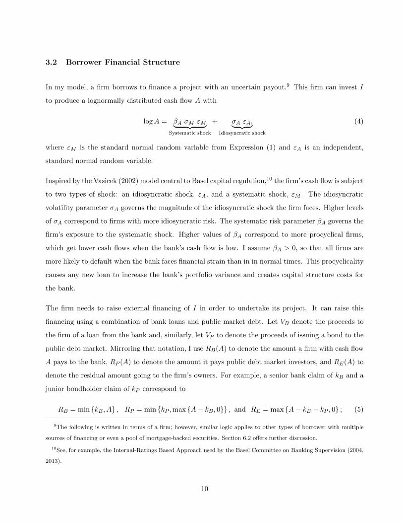
3.2 Borrower Financial Structure

In my model, a firm borrows to finance a project with an uncertain payout.9 This firm can invest I

to produce a lognormally distributed cash flow A with

logA = βA σM εM︸ ︷︷ ︸Systematic shock

+ σA εA,︸ ︷︷ ︸Idiosyncratic shock

(4)

where εM is the standard normal random variable from Expression (1) and εA is an independent,

standard normal random variable.

Inspired by the Vasicek (2002) model central to Basel capital regulation,10 the firm’s cash flow is subject

to two types of shock: an idiosyncratic shock, εA, and a systematic shock, εM . The idiosyncratic

volatility parameter σA governs the magnitude of the idiosyncratic shock the firm faces. Higher levels

of σA correspond to firms with more idiosyncratic risk. The systematic risk parameter βA governs the

firm’s exposure to the systematic shock. Higher values of βA correspond to more procyclical firms,

which get lower cash flows when the bank’s cash flow is low. I assume βA > 0, so that all firms are

more likely to default when the bank faces financial strain than in in normal times. This procyclicality

causes any new loan to increase the bank’s portfolio variance and creates capital structure costs for

the bank.

The firm needs to raise external financing of I in order to undertake its project. It can raise this

financing using a combination of bank loans and public market debt. Let VB denote the proceeds to

the firm of a loan from the bank and, similarly, let VP to denote the proceeds of issuing a bond to the

public debt market. Mirroring that notation, I use RB(A) to denote the amount a firm with cash flow

A pays to the bank, RP (A) to denote the amount it pays public debt market investors, and RE(A) to

denote the residual amount going to the firm’s owners. For example, a senior bank claim of kB and a

junior bondholder claim of kP correspond to

RB = min {kB, A} , RP = min {kP ,max {A− kB, 0}} , and RE = max {A− kB − kP , 0} ; (5)

9The following is written in terms of a firm; however, similar logic applies to other types of borrower with multiple

sources of financing or even a pool of mortgage-backed securities. Section 6.2 offers further discussion.

10See, for example, the Internal-Ratings Based Approach used by the Basel Committee on Banking Supervision (2004,

2013).

10

pari-passu debt claims of kB for the bank and kP for the bondholders correspond to

RB = min

{kB,

kBkB + kP

A

}, RP = min

{kP ,

kPkB + kP

A

}, and RE = max {A− kB − kP , 0} ; (6)

and equity claims entitling the bank to kB fraction of the firm’s return and the bondholders to kP

fraction of the firm’s return correspond to

RB = kBA, RP = kPA, and RE = (1− kB − kP )A. (7)

I assume that the public debt market claim, RP ; the bank claim, RB; and the residual claim, RE , are

all non-negative and non-decreasing functions of the firm’s cash flow value.11 This includes almost all

contracts used in practice, including the previously mentioned sets. Put options and money burning

contracts do not satisfy these restrictions. Contracts where the borrower’s repayment depends on

the performance of the bank’s in-place assets are also excluded. However, neither class of contract is

common in corporate fund raising.12

Seniority is a central concept in this paper. Formally, I define seniority as follows:

Definition 1 Repayment RB is senior if RB = min{A, kB} for some kB ≥ 0.

This captures the conventional notion of seniority: senior contracts are paid first in bankruptcy. For

example, the ‘senior’ claim RB in Expression (5) is senior for any kB.

3.3 Bank-Level Capital Structure Costs Created by Lending

Both banks and public debt market investors can finance the firm. When a bank lends to the firm,

financing the new loan creates capital structure frictions for the bank. This section quantifies the

marginal bank-level capital structure frictions created by originating a new loan.

11The common requirement that claims are non-decreasing follows naturally if a firm’s financiers can sabotage its value

(DeMarzo, Kremer, and Skrzypacz 2005).

12Although I explicitly consider bank-level capital structure frictions, I have ignored borrower-level frictions. I have

also ignored the possibility of absolute priority rule violations. Both of these frictions can be conceptualized as limits to

the set of possible bank repayment contracts. Limiting the contracting space in that manner does not change the core

result.

11

Consider the bank’s capital structure frictions if it holds not only its in-place assets, but also a new

loan to the firm. Making a new loan increases the bank’s cash flow from B to B+RB(A) and increases

the bank’s value from Expression (3) to

W (B +RB (A)) = E [B +RB(A)]− E [max {E [B +RB (A)]−B −RB (A) , 0}] (8)

Adding a new loan to the bank’s assets always increases the bank’s value. However, that increase is

less than the loan’s expected repayment, because holding a new loan adds risk to the bank’s portfolio.

That risk creates bank-level frictions, which eat up part of the loan proceeds. I write ∆ (RB (A)) as

the intermediary capital structure frictions created by a new loan with repayment RB(A):

∆ (RB (A)) = E [RB(A)]︸ ︷︷ ︸Expected loan repayment

− W (B +RB(A))︸ ︷︷ ︸Bank value with the new loan

+ W (B)︸ ︷︷ ︸Bank value without the new loan

(9)

=E [max {E [B +RB (A)]−B −RB (A) , 0}]︸ ︷︷ ︸Capital structure frictions with loan

− E [max {E [B]−B, 0}] .︸ ︷︷ ︸Capital structure frictions without loan

(10)

Because the borrower is procyclical, the borrower’s loan repayment is also procyclical. Procyclical

loans repay less in the states of the world where the bank needs cash to avoid punishment. That

means that making a loan always increases the bank’s capital structure frictions, as shown by the

following lemma:

Lemma 1 Making a loan increases the bank’s expected capital structure costs, unless that loan’s re-

payment is always zero.

Importantly, senior contracts create lower bank-level capital structure cost than more junior contracts.

A junior contract is more exposed to firm default risk than a senior contract, and therefore loses more

value in bad states of the world. Those losses make junior debt more procyclical and create greater

distress costs for a bank holding it. Lemma 2 formalizes this intuition.

Lemma 2 A bank loan contract that is senior (in the sense of Definition 1) produces lower bank-level

capital structure costs than any other bank loan contract with the same expected repayment.

A highly procyclical borrower leads to increased bank capital structure costs for the same reason that

a junior loan contract does. When the bank has a low cash flow, a highly procyclical borrower also has

12

a low cash flow and cannot repay its loans. Thus, a bank holding loans written by a highly procyclical

borrower faces higher distress costs in bad states of the world. The opposite applies to borrowers that

are less procyclical. These borrowers retain their value in bad times and create less capital structure

costs for their lender. In the Diamond (1984) case where borrowers have only diversifiable idiosyncratic

risk, the bank can take on very high leverage with little risk of distress. However, if borrowers have do

systematic risk, high bank leverage can lead to substantial bank distress costs. Lemma 3 states this

relationship between procyclicality and bank-level capital structure cost more formally:

Lemma 3 Consider two borrowers, C and D, where

1. Borrower C has more systematic risk than borrower D, βCA > βDA ;

2. Borrower C has less idiosyncratic risk than borrower D, σCA < σDA , such that the cash flows of

borrowers C and D have the same total variance, σCA2

+ σ2Mβ

CA

2= σDA

2+ σ2

MβDA

2; and

3. Borrowers C and D are otherwise identical.

Any bank loan contract with a greater than zero repayment produces higher bank-level capital struc-

ture costs if written on borrower C’s cash flow, RB(AC), than if written on borrower D’s cash flow,

RB(AD).

Another way to see the importance of procyclicality is to consider a bank that is large relative to the

individual loans it originates. This abstracts from “concentration” or “single name” risk and focuses

on loan-level systematic risk.13 As Lemma 4 shows, a large bank cares only about a loan’s systematic

risk and ignores loan-specific idiosyncratic risk:

Lemma 4 As the bank’s initial size, B0, increases, the incremental bank-level capital structure cost

created by a new bank loan, ∆ (RB (A)), converges to a simple covariance expression:

∆ (RB (A)) → P [B < E [B]](E [RB (A)]− E

[RB(A)

∣∣B < E [B]] )

(11)

= COV[RB(A), I [B ≥ E [B]]

]. (12)

13This large bank assumption contrasts with the illustrative example in Section 2, where I ignore the risk from the bank’s

in-place assets and focus only on borrower’s risk. Here, conversely, a large bank is indifferent to a loan’s idiosyncratic

risk.

13

Expression (12) has an intuitive interpretation. Capital structure costs arise from punishing the banker

in bad states of the world. The amount of excess punishment created by making a new loan is equal

to the probability of a punishment multiplied by the amount that the new loan increases the severity

of that punishment. Loans that are likely to default in bad states of the world create high frictions;

loans that are likely to repay create lower frictions.

Expression (12) also includes a covariance formulation of capital structure costs. This expression is

analogous to the covariance formulations in modern portfolio theory. There, an investor evaluating a

small new investment does not care about that investment’s idiosyncratic risk and instead considers

only its expected return and its covariance with the investor’s existing portfolio. Here, a bank with a

large number of loans does not care about a new loan’s idiosyncratic risk, and instead considers only

its expected repayment and systematic risk. What matters to the bank is the extent to which the new

loan repays in the states of the world where the bank has low cash flows and faces distress costs.14

3.4 Bank Lending Technology

The bank has a unique lending technology that creates value for its borrowers. Public debt markets

cannot directly use this technology due either to diffuse ownership (as in Diamond (1984)) or confiden-

tiality issues (as in Campbell (1979)). Thus, the only way a firm can get the benefits of this lending

technology is to take out a bank loan.

Papers such as Diamond and Verrecchia (1991) and Holmstrom and Tirole (1997) argue that banks

monitor borrowers and attenuate moral hazard. This section lays out a similar model, where banks

create value by preventing the firm’s managers from taking a value destroying action that confers

private benefits. This value destroying action could be shirking, risk shifting, or simply stealing.15 If

a bank has lent a firm a large amount of money, other investors can have confidence that the bank has

14I assume that the bank cannot sell its in-place assets to reduce risk; however, allowing such asset sales would not

matter under an intuitive model of bank asset preferences. By a similar envelope theorem argument, a large bank that

initially held an optimal mix of assets does not substantially alter its asset mix in response to a single new loan.

15My results extend to other bank technologies. The analysis in Section 4.2 applies to any model where the benefit of

a bank loan is proportional to its size and Section 5.3 explicitly looks at a screening technology that reduces asymmetric

information.

14

prevented moral hazard. That certification effect reduces the interest rate the firm pays on its other

debt.16 The borrower in this model is fully aware of these effects and willing to pay more for a bank

loan in order to reduce its total financing cost.

The firm’s cash flow is A1, as in Expression (4). If the firm’s managers take the value destroying

action, that cash flow is reduced to A0, which is lower or riskier. This value destroying action reduces

the value of any claim the firm can issue:

∀RB, E [RB(A1)] ≥ E [RB(A0)] . (13)

The bank can pay cost M to monitor the firm and prevent the value destroying action. However, the

bank’s monitoring action is not observable, which means the bank only monitors if it has sufficient

skin in the game. The following section builds up a game where a bank with capital structure frictions

must be provided incentives.

3.5 Timeline and Strategies

Firm debt structure arises from a game played by a firm, a bank, and a bond investor. As described in

the previous sections, the bank has capital structure frictions and a monitoring technology, while the

bond investor has no capital structure costs but cannot monitor. The firm has to raise financing for an

investment of I from the bank and the bond investor. I model the process of raising this investment

and the bank’s moral hazard about its monitoring action, m, as follows:

In step 1, the firm, the bank, and the bond investor engage in bargaining to select a financing contract

C = (VB, RB, VP , RP ). This contract includes a bank loan (with proceeds VB and repayment RB) and

a bond (with proceeds VP and repayment RP ). The bargaining can take any form, as long as it selects

Pareto efficient contracts. For example, the parties could engage in Nash bargaining or the firm could

make a take-it-or-leave-it offer.

16Papers such as Ramakrishnan and Thakor (1984), Fama (1985), Diamond and Verrecchia (1991), Datta, Iskandar-

Datta, and Patel (1999), Sufi (2007), and Ongena, Roscovan, Song, and Werker (2007) support this view that bank loans

provide certification.

15

Figure 2: Timeline of Monitoring Game

Figure 2 shows a timeline for the monitoring game described in Section 3.5.

1 Pareto efficient bank loan and bond contract, C, selected through bargaining.

2 Bank chooses whether to shirk or monitor, m ∈ {0, 1}.

3 Payoffs realized.

In step 2, the firm invests I into a project if sufficient financing was raised, VB + VP ≥ I. If sufficient

financing was not raised, the game ends and all agents get zero payoff. After the investment is made,

the bank chooses whether to shirk or to pay M to monitor and prevent the value destroying action. If

the bank monitors, m = 1, the firm’s cash flow is A1. If the bank shirks, m = 0, the firm’s management

take the value destroying action and the firm’s cash flow A0.

In step 3, the firm’s cash flow Am is realized and is used to repay the bank, RB(Am), and the bond

investor, RP (Am). Based on the bond and loan contracts, C = (VB, RB, VP , RP ), and the bank’s

action, m, the firm gets an expected payoff of

πE(C,m) = E[Am − I︸ ︷︷ ︸Project

+VP −RP (Am)︸ ︷︷ ︸Bond

+VB −RB(Am)︸ ︷︷ ︸Loan

], (14)

the bank gets an expected payoff of

πB(C,m) = E[−VB +RB(Am)︸ ︷︷ ︸

Loan

− ∆(RB(Am))︸ ︷︷ ︸Capital structure cost

− mM︸︷︷︸Monitoring cost

], (15)

and the bond investor gets an expected payoff of

πP (C,m) = E[−VP +RP (Am)︸ ︷︷ ︸

Bond

]. (16)

(For simplicity, I set the risk-free interest rate to zero.)

If the payoff to shirking is less than the payoff to monitoring, the bank monitors the firm. I call this

the bank’s incentive compatibility condition:

πB(C, 0) ≤ πB(C, 1)⇔ M︸︷︷︸Cost of monitoring

≤ E [RB(A1)−RB(A0)]︸ ︷︷ ︸Repayment lost by shirking

− ∆ (RB(A1)) + ∆ (RB(A0)) .︸ ︷︷ ︸Capital structure cost from shirking

(17)

16

This expression has an intuitive interpretation. For the bank to monitor, the cost of monitoring must

be less than the losses the firm’s value destroying action creates for the bank.

A strategy profile is a financing contract and a monitoring action pair, (C,m). I call a strategy profile

incentive compatible if taking the action m maximizes the bank’s expected payoff given financing

contract C, so that πB(C,m) = max{πB(C, 0), πB(C, 1)}. I call an incentive compatible strategy

profile (C,m) Pareto efficient if any other incentive compatible strategy profile, (C ′,m′), that delivers

a higher expected payoff to one or more agents, πi(C′,m′) > πi(C,m), must also deliver a lower payoff

to one or more agents, πj(C′,m′) > πj(C,m).

The following sections show that any Pareto efficient strategy profile makes the bank senior. As such,

any bargaining process that produces Pareto efficient contracts can be used in step 1 of the game.

Pareto efficiency is a natural property of bargaining games. For example, it emerges if the parties

engage in asymmetric Nash bargaining to maximize the generalized Nash product,

πE(C,m)αEπB(C,m)αBπP (C,m)1−αE−αB , (18)

for some bargaining power parameters αE , αB, and 1 − αE − αB in (0, 1). Pareto efficient contracts

also emerge if the firm makes a take-it-or-leave-it offer of a contract to the bank and the bond market.

Such a take-it-or-leave-it offer always results in a Pareto efficient contract because varying VB and VP

allow the firm to extract the entire surplus.

4 Borrower Procyclicality and Bank Seniority

This section contains my key results on seniority and procyclicality. Section 4.1 lays the groundwork

by characterizing the Pareto efficient financing contracts. Section 4.2 shows that the bank is senior if

firms that are not monitored repay nothing. Section 4.3 extends that seniority result to a setup where

bank monitoring increases the mean or decreases the variance of firm cash flows. Section 4.4 looks at

how procyclicality leads firms to shift from bank loans to bonds or even to forgo investment entirely.

17

4.1 Pareto Efficient Financing Contract

Three types of financing contract can be Pareto efficient and so are possible in equilibrium. First,

monitored investment where the firm takes a bank loan and is monitored. Second, unmonitored

investment where the firm funds its investment entirely by bond issuance, forgoing monitoring. Third,

no investment where the firm simply does not invest. Each of these types of financing contract has

distinct properties:

Theorem 1 Any contract used in equilibrium maximizes the total payoff Π = πE + πB + πP . The

equilibrium is of one of three types:

1. Monitored Investment: The firm borrows from the bank and the bond market. The bank

repayment, RB, minimizes bank capital structure costs, ∆(RB), while ensuring monitoring is

incentive compatible for the bank, Expression (17). This contract leads to a total payoff of

ΠM = πE + πB + πP = E [A1]−∆(RB(A1))−M. (19)

2. Unmonitored Investment: The firm issues a bond that finances its investment. The bank

does not monitor and does not get any repayment. This contract leads to a total payoff of

ΠU = E [A0]− I.

3. No Investment: The firm is unable to raise financing and the project does not occur. Because

a contract is not reached, the total payoff is ΠN = 0.

Sections 4.2, 4.3, and 4.4 use these equilibria to look at firm debt structure and at procyclicality.

4.2 Banks Are Senior When Firms That Are Not Monitored Repay Nothing

To discuss the efficiency of bank seniority, I need to impose a functional form on the impact of bank

monitoring. For simplicity, I first consider a case where the firm absconds with the financing proceeds

if the bank does not monitor. So a firm that is not monitored has a cash flow equal to zero, A0 = 0.

In this case, the bank’s incentive compatibility condition, Expression (17), simplifies to

M︸︷︷︸Cost of monitoring

≤ E [RB(A1)−∆(RB(A1))] .︸ ︷︷ ︸Value of firm’s repayment

(20)

18

This expression shows that the bank’s monitoring decision depends on how the cost of monitoring

compares with the value of the loan. A large loan gives the bank more skin in the game, which makes

the bank more willing to monitor. Theorem 2 shows that making the bank senior is the optimal way

to provide those incentives:

Theorem 2 If firms repay nothing when not monitored, the bank is senior in all Pareto efficient

contracts.

The intuition here follows directly from Lemma 2: senior repayments minimize bank capital structure

costs. To illustrate this, consider a firm with senior, subordinated, and junior classes of debt, each

with a promised repayment of $0.10. Figure 3 shows the bank-level capital structure frictions created

for a bank that holds each of these classes. It also shows the cost of a hypothetical risk-free claim.

Figure 3: Impact of Seniority on Bank-Level Capital Structure Costs

Figure 3 illustrates how different claims on a firm create different bank-level financing costs. The x-

axis compares investments four claims with varying seniority: (1) a hypothetical risk-free investment,

(2) a senior debt claim with a face value of $0.10, (3) a subordinated debt claim with a face value

of $0.10 which is subordinated to the senior claim, (4) a junior debt claim with a face value of $0.10

which is subordinated to both the senior and subordinated claims. The white bars show the capital

structure cost created for a bank holding each claim. The model in Section 4.3 is used for this chart

with σ2A + β2

Aσ2M = 2, ρ =

β2Aσ

2M

σ2A+β2

Aσ2M

= 0.2, µH = 0, and σ2H = 0.4.

$0.00

$0.01

$0.10 Risk-Free

Debt

$0.10 Senior

Firm Debt

$0.10 Subord.

Firm Debt

$0.10 Junior

Firm Debt

Bank Capital Structure Cost

Senior contracts produce lower bank-level capital structure costs because these contracts have less

systematic risk. On the left of Figure 3, a risk-free claim produces no capital structure cost for the

19

bank. Such a claim does not lose value in bad states of the world and so it does not increase the

bank’s probability of distress. On the right, a junior debt claim produces high capital structure costs.

A junior claim loses much of its value in bad states of the world and so is worth little when the bank

needs capital to avoid distress.

Seniority impacts capital structure costs by influencing contracts’ procyclicality. As in Lemma 4,

capital structure costs are higher for more procyclical contracts. Junior debt repayments are highly

procyclical because they pay a higher interest rate in good states of the world and are less likely to pay

out in bad states of the world. That procyclicality makes it expensive for the bank to finance these

contracts, which causes the bank to charge a much higher interest rate than the public debt markets

would. Seniority insulates loans from economic shocks and makes them less procyclical. This makes

them cheaper for the bank to hold, which reduces the excess interest rate the bank charges.

Theorem 2 can be extended to show that the bank is senior whenever a borrower needs a bank loan

with a certain value. Thus, bank seniority is optimal whenever the benefit of a bank loan is dependent

on the loan size. For example, if a firm can borrow only through bank loans, it makes those loans

senior to equity in order to minimize lender-level frictions. This provides a complementary explanation

to theoretical works such as Townsend (1979) or Gale and Hellwig (1985). Another example could

be a relationship lending model where a certain bank loan size is necessary to maintain a banking

relationship. There, the bank loan should be senior to minimize the costs of that relationship lending.

4.3 Banks Are Senior When Monitoring Makes Cash Flows Larger or Less Risky

In Section 4.2, bank shirking hurts senior creditors just as much as junior creditors. In practice, junior

claimants often bear the brunt of the consequences of bad lending decisions. This section considers

a model where bank shirking disproportionately impacts junior creditors. Perhaps surprisingly, bank

seniority again emerges, even though this seniority weakens bank incentives. Efficient contracts give

the bank a sufficiently large senior claim, which preserves bank incentives while minimizing capital

structure costs.

20

Suppose that instead of having no cash flow, unmonitored firms have a cash flow, A0, with lower mean

or higher variance:

logA0 = logA1 − µH︸︷︷︸Reduced mean

+ σHεH ,︸ ︷︷ ︸Additional risk

(21)

where µH ≥ 0 controls how monitoring increases cash flows, σH controls how monitoring reduces risk,

and εH is a standard normal and independent shock. The reduced mean is due to shirking, stealing,

or diverting cash flows and reduces the value of all claims, debt and equity alike. The added variance

is due to risk shifting or negligence by the firm and reduces the value of debt-like claims.

In this section, I assume that the bank is large relative to the borrower. This assumption is intuitive,

unlikely to change the model results, and eases calculation by removing idiosyncratic loan risk, as

in Lemma 4. I also prohibit firms from issuing equity-like claims to creditors. Specifically, I assume

that the firm cannot issue contracts to the bank or bond investor that have a greater than 50%

chance of defaulting. This restricts the firm to debt-like contracts that reach their highest payoff for

firm cash flows below 1, and so is equivalent to imposing that RB(1) ≥ RB and RP (1) ≥ RP . This

follows naturally from a model where firm-level default costs make extremely high leverage suboptimal.

This assumption ensures Expression (13) holds and that unmonitored firms are worse for creditors.

Importantly, this assumption does not prevent the firm from making the bank junior to bondholders.

Under this setup, and in contrast to the previous section, junior claims lose more than senior claims if

the bank fails to monitor. Figure 4 shows the degree to which monitoring increases the value of claims

with the same repayment but varying seniority. I call this bank incentives, as it is the amount that

the bank’s claim value is impaired if it shirks.

On the left of the figure, very senior claims generate weak bank incentives because these contracts will

pay off with almost certainty regardless of whether the bank monitors. More junior claims produce

stronger incentives, because the value of junior debt is more sensitive to an increase in variance or

decrease in mean, as junior claims lose the most when the firm defaults. However, seniority remains

efficient even though it weakens bank incentives:

Theorem 3 If monitoring increases the mean of firm cash flows or decreases the variance of firm

cash flows or both, the bank is senior in all Pareto efficient contracts.

21

Figure 4: Impact of Seniority on Bank Incentives

Figure 3 illustrates how different claims on a firm create different bank-level financing costs. The x-

axis compares investments four claims with varying seniority: (1) a hypothetical risk-free investment,

(2) a senior debt claim with a face value of $0.10, (3) a subordinated debt claim with a face value

of $0.10 which is subordinated to the senior claim, (4) a junior debt claim with a face value of $0.10

which is subordinated to both the senior and subordinated claims. The black bars show the amount

that shirking reduces the payoff of each claim. The model in Section 4.3 is used for this chart with

σ2A + β2

Aσ2M = 2, ρ =

β2Aσ

2M

σ2A+β2

Aσ2M

= 0.2, µH = 0, and σ2H = 0.4.

$0.00

$0.01

$0.10 Risk-Free

Debt

$0.10 Senior

Firm Debt

$0.10 Subord.

Firm Debt

$0.10 Junior

Firm Debt

Bank Incentives (Amount Bank Loses If It Shirks)

A sufficiently large senior claim creates appropriate bank incentives while minimizing capital structure

costs. This holds because senior debt produces the most bank incentive per dollar of capital structure

cost. Switching the bank from a small junior claim to a large senior claim preserves bank incentives

while reducing capital structure costs.

Returning to the example of a firm with three classes of debt, Figure 5 compares the capital structure

cost and bank incentives created by each class. The first three claims have the same face value and

varying seniority. A small junior debt contract gives banks good incentives, but it also creates high

capital structure costs. A small senior debt contract has greatly reduced capital structure costs, but

weak incentives. A small subordinated contract lies between these two.

The fourth claim is larger and senior, it is a $0.20 senior claim, which has a payoff equal to the sum

of the payoff of $0.10 the senior claim and the payoff of the $0.10 subordinated claim. The capital

structure cost for this large senior claim is the sum of the capital structure cost of the two smaller

22

Figure 5: A Large Senior Claim Versus a Small Junior Claim

Figure 5 illustrates how varying the size and seniority of the bank loan impacts bank incentives and

capital structure costs. The x-axis has four claims with varying seniority and varying size: (1) a

senior debt claim (marked with A) with a face value of $0.10 , (2) a subordinated debt claim (B)

with a face value of $0.10 that is subordinated to $0.10 of repayment, (3) a junior debt claim (C)

with a face value of $0.10 that is subordinated to $0.20 of repayment, and (4) a senior firm claim

with a face value of $0.20, whose payoff is the sum of the payoffs of the $0.10 senior claim and the

$0.10 subordinated claim. The black bar shows the amount that bank monitoring increases the value

of each claim. The white bar shows the bank-level capital structure cost created for a bank holding

each claim. The dashed line shows the bank’s cost of monitoring, M . The model in Section 4.3 is

used for this chart with σ2A + β2

Aσ2M = 2, ρ =

β2Aσ

2M

σ2A+β2

Aσ2M

= 0.2, µH = 0, and σ2H = 0.4.

$0.00

$0.01

$0.10 Senior

Firm Debt

$0.10 Subord.

Firm Debt

$0.10 Junior

Firm Debt

$0.10 Senior +

$0.10 Subord.

Capital Structure Cost Bank Incentives

AA'

BB'

C

C'

B'

B

AA'

claims, and it similarly provides incentives equal to the sum of the incentives produced by those two

claims. This large senior claim produces stronger incentives than the smaller junior claim, while having

lower capital structure cost. As in Theorem 3, a large senior claim can provide sufficient incentives

with low capital structure cost.

The intuition here is that the bank is punished when the loan contract denies it a repayment. This

punishment encourages good behavior; however, it creates a deadweight loss of bank-level capital

structure costs in states of the world where the bank has low capital. The most effective contract

punishes in the states of the world when the agent clearly shirked. A large senior contract does that

in my model by applying large losses when the bank is most likely to have shirked.

23

Figure 6 illustrates this by showing how the firm’s cash flow realization impacts both the probability

the bank monitored and the amount of losses borne by senior and junior creditors. Senior loans

punish the bank when the firm fails catastrophically and the bank is most likely to have shirked.

Junior contracts punish the bank whenever the firm fails, which punishes a larger fraction of those

banks that did shirk, but also punishes many banks that did not shirk. If the firm just barely defaults,

it may be due to a bad lending decision or simply bad luck. Punishing banks from the first dollar of

firm losses punishes many banks that did not shirk and creates a deadweight loss. A large senior loan

is efficient because it delivers a large punishment in precisely the states where the bank is most likely

to have shirked.

Figure 6: Crime and Punishment

Figure 6 illustrates how varying the firm’s cash flow realization impacts both the probability that the

bank shirked and the amount of losses incurred on a small junior and a large senior debt claim. The

firm’s cash flow, Am, is plotted on the x-axis. On the left axis, a solid line plots the likelihood ratio,

the probability of each firm value given the bank monitored divided by the probability of that firm

value given the bank shirked. On the right axis, a dashed line plots the loss taken on a senior claim

with a face value of $0.20. A dashed line plots the loss taken on a claim with a promised repayment

of $0.10 that is junior to the $0.20 senior claim. The model in Section 4.3 is used for this chart with

σ2A + β2

Aσ2M = 2, ρ =

β2Aσ

2M

σ2A+β2

Aσ2M

= 0.2, µH = 0, and σ2H = 0.4.

$0.00

$0.05

$0.10

$0.15

$0.20

0%

50%

100%

$0.00 $0.10 $0.20 $0.30 $0.40

Loss o

n L

oan C

ontracts

Lik

elihood R

atio

Firm Cash Flow

Likelihood Ratio

Loss on $0.20

Senior Debt

Loss on $0.10

Junior Debt

This relies on the fact that the probability that the bank shirked is decreasing in the firm’s realized

cash flow. This likelihood ratio property is natural, and means that it is optimal to punish the bank

in the states of the world where the firm value is lowest. Under a different model where monitoring

24

increased firm risk, my results would not hold. For example, suppose that a monitored firm has a

lognormal payout A1, as before, and that an unmonitored firm always pays out half of the investment

amount, A0 = 12I. With those assumptions, the bank is not senior in equilibrium. A senior claim would

produce no incentives for the bank, because bank shirking never hurts senior creditors. As a result,

the bank would take on a junior claim. This may parallel venture capital funds. Venture capital

backed companies primarily issue convertible preferred equity, which gains most of its value from

upside scenarios. This matches a world where venture capital funds actively manage their investments

to maximize their risk and their return.

Not shown on Figure 6, the probability that the bank is in financial distress is higher in states of the

world where the firm does poorly. This reduces the efficiency of senior contracts, as they punish more

in states of the world where the firm does most poorly and the bank is more likely to face capital

structure costs. This is akin to an insurance effect in other contracting models with risk averse agents.

Nevertheless, as Theorems 2 and 3 show, the likelihood ratio effect discussed previously dominates

this insurance effect.

4.4 Procyclicality and the Choice of Bank Debt or Bonds

Theorem 1 showed that there were three types of equilibria: monitored investment, unmonitored

investment, and no investment. This section looks at how the equilibrium financing contract varies as

the model parameters change. I show that as borrower procyclicality increases, firms substitute from

monitored investment to either unmonitored investment or no investment.

Both monitored and unmonitored investing create frictions. Bank loans create monitoring costs and

bank-level financial frictions. Bond issuance without a bank loan creates moral hazard costs. The firm

issues bank debt rather than solely bonds if the payoff from monitored investment is higher than the

payoff from unmonitored investment. This happens when the moral hazard frictions are greater than

the capital structure cost frictions:

ΠM ≥ ΠU ⇔M + ∆ (RB(A)) ≤ E [A1 −A0] , (22)

where RB is set according to Expression (17). A firm is locked out of the financing market when both

sets of frictions are so severe that it cannot raise money.

25

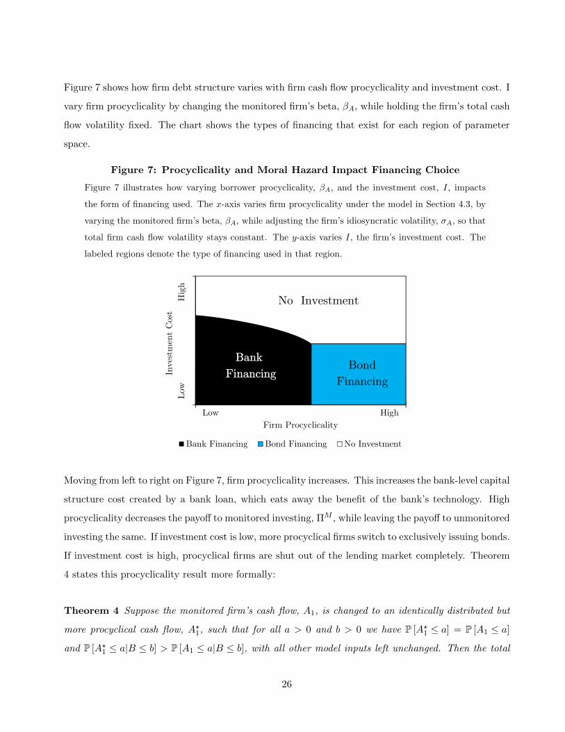
Figure 7 shows how firm debt structure varies with firm cash flow procyclicality and investment cost. I

vary firm procyclicality by changing the monitored firm’s beta, βA, while holding the firm’s total cash

flow volatility fixed. The chart shows the types of financing that exist for each region of parameter

space.

Figure 7: Procyclicality and Moral Hazard Impact Financing Choice

Figure 7 illustrates how varying borrower procyclicality, βA, and the investment cost, I, impacts

the form of financing used. The x-axis varies firm procyclicality under the model in Section 4.3, by

varying the monitored firm’s beta, βA, while adjusting the firm’s idiosyncratic volatility, σA, so that

total firm cash flow volatility stays constant. The y-axis varies I, the firm’s investment cost. The

labeled regions denote the type of financing used in that region.

Bank Financing Bond Financing No Investment

No Investment

Bond

Financing

Inves

tmen

t C

ost

Low

Hig

h

Bank

Financing

Low High

Firm Procyclicality

Moving from left to right on Figure 7, firm procyclicality increases. This increases the bank-level capital

structure cost created by a bank loan, which eats away the benefit of the bank’s technology. High

procyclicality decreases the payoff to monitored investing, ΠM , while leaving the payoff to unmonitored

investing the same. If investment cost is low, more procyclical firms switch to exclusively issuing bonds.

If investment cost is high, procyclical firms are shut out of the lending market completely. Theorem

4 states this procyclicality result more formally:

Theorem 4 Suppose the monitored firm’s cash flow, A1, is changed to an identically distributed but

more procyclical cash flow, A?1, such that for all a > 0 and b > 0 we have P [A?1 ≤ a] = P [A1 ≤ a]

and P [A?1 ≤ a|B ≤ b] > P [A1 ≤ a|B ≤ b], with all other model inputs left unchanged. Then the total

26

payoff of monitored investing, ΠM , decreases while the total payoff of unmonitored investing, ΠU , stays

constant. As a result, the firm may transition from bank lending to bond issuance or no investment.

The above analysis fixes firm debt levels; however, similar results hold if firm leverage and bank effort

intensity are set endogenously. Procyclicality increases a firm’s marginal cost of bank borrowing and

the marginal cost of the bank’s technology. The firm responds by decreasing its bank loan size and

forgoing certification. If public market borrowing depends on that certification, the firm also reduces

its non-bank borrowing.

5 Alternative Financial Frictions and Bank Technologies

This section extends my model to different lending technologies and different bank-level frictions.

Section 5.1 extends my results to a model that uses bank-level distress and tax costs in place of

Diamond (1984) financing frictions. Section 5.2 shows bailouts can act as a complementary mechanism.

Section 5.3 shows that seniority also emerges from a model where the bank screens against low quality

borrowers. For simplicity, I consider capital structure costs for a large, diversified bank for each of

these extensions. As in Lemma 4, this removes the impact of idiosyncratic loan risk.

5.1 Taxes and Distress Costs as Bank Capital Structure Frictions

My results extend to the trade-off theory frictions of tax benefits of debt and financial distress costs.

These frictions produce the same results as the Diamond (1984)-style frictions I use in other sections

of the paper.

A stylized empirical fact is that banks overwhelmingly prefer debt financing. I use a tax benefit of

debt to make bank equity privately expensive and to drive high bank leverage. Trading off tax benefits

against distress costs is in line with an expansive capital structure literature. As applied to banks,

Gornall and Strebulaev (2014) argue that tax costs can explain high bank leverage and Schandlbauer

(2013) and Schepens (2013) show empirically that financial institutions vary their leverage in response

to tax changes. Nevertheless, other debt benefits could equally well motivate bank leverage. For

example, a liquidity provision benefit (such as DeAngelo and Stulz (2013)) or a clientele effect (such

27

as Baker and Wurgler (2013)) could lead to similar formulations. Any of these frictions give banks an

incentive to increase leverage and become fragile.

The bank’s gross tax cost is τB, where τ > 0 is a linear tax rate applied to the bank’s cash flow of

B. Issuing debt can shield the bank from this tax burden. If the bank issues debt with a promised

repayment of S, it receives an interest tax shield equal to the lesser of τS and its total tax bill.17

Taking into account both the bank’s gross tax bill and its interest tax shield, the bank’s net tax cost

is τB − τ min{B,S}.

Debt provides a tax shield; however, it makes the bank vulnerable to financial distress. I model this

cost either as proportional to the bank’s debt repayment shortfall or of fixed size.

First, I model bank financial distress as a costly fire sale to raise liquidity. If a bank’s cash flow is low,

it meets its debt repayment by selling illiquid assets for less than the value these assets would have if

held to maturity. The bank’s monitoring technology provides a natural motivation of such costs. If

the bank sells a loan, the associated firm takes a value destroying action. Thus when the bank sells

loans, value is destroyed though increased borrower moral hazard.18 Alternatively, this friction could

be viewed as the cost of raising equity at an inopportune time.

If the bank’s cash flow is less than its promised debt repayment, the bank must raise S −B by selling

illiquid assets. In order to raise $1 for debt repayment, the bank must sell assets that would be worth

$(1 + α) if held to maturity. The cost of this fire sale is equal to αmax {S −B, 0} for some linear fire

sale cost α > 0. When the promised debt repayment is set optimally, the bank’s value after taxes and

these distress costs, Wα(B), is

Wα(B) = supS

{E [B]︸ ︷︷ ︸

Cash flow

− τE [B]︸ ︷︷ ︸Gross tax

+ τE [min{B,S}]︸ ︷︷ ︸Tax shield

−αE [max{S −B, 0}]︸ ︷︷ ︸Distress cost

}. (23)

Second, I consider a distress cost of a fixed size that is incurred if the bank’s cash flow is less than

its debt repayment. This cost is either a direct bankruptcy cost or the cost of the loss of customers,

employees, and suppliers associated with financial distress. Managerial incentives offer an alternative

17This tax formulation is used for simplicity. The same results hold if the interest tax deduction is based on the interest

cost implied by the debt repayment.

18Bank distress would then have a knock-on effect on public debt market participants. This effect could be priced into

public debt offerings and bank seniority would persist.

28

explanation for distress costs. If managers face a penalty for poor performance (for example, suppose

they get fired), a self-interested manager would seek to minimize the probability of financial distress.

Suppose that if B < S, the bank incurs a distress cost of γB0 for some γ > 0. The bank’s value,

W γ(B), for the optimal promised debt repayment, S, is

W γ(B) = supS

{E [B]︸ ︷︷ ︸

Cash flow

− τE [B]︸ ︷︷ ︸Gross tax

+ τE [min{B,S}]︸ ︷︷ ︸Tax shield

− γB0P [B < S]︸ ︷︷ ︸Distress cost

}. (24)

With either form of distress cost, I define the bank capital structure cost created by a new loan, ∆,

as before using Expression (9). The game in Section 3.5 can be easily updated to this form of distress

cost, with similar equilibria holding. Under a model where unmonitored borrowers abscond with the

cash flow, as in Section 4.2, the bank is always senior:

Theorem 5 If unmonitored borrowers repay nothing and the bank has either fixed or proportional

distress costs, the bank is senior in all equilibria.

As before, making the bank senior minimizes the bank’s asset portfolio risk, which in turn minimizes

bank-level distress costs. Junior securities produce more tax costs in good states of the world and

more distress costs in bad states of the world. Senior securities are less procyclical and thus less costly

for the bank to hold.

If, as in Section 4.3, bank monitoring increases borrower quality or decreases borrower risk, the bank

is senior for reasonable model parameters. To illustrate, I use a baseline parameter set motivated by

empirical proxies and vary parameters from that baseline one by one.

My baseline uses a one-year loan and a firm volatility of 40%, consistent with Choi and Richardson

(2008) and Schaefer and Strebulaev (2008). I set the correlation between the bank and firm to 45%,

in line with the Basel Committee on Banking Supervision (2004, 2013) which uses values ranging from

28% to 49%.19 I use a bank asset volatility of 3%, in line with Ronn and Verma (1986) and Hassan,

Karels, and Peterson (1994). Finally, I use a tax rate of 20% to model the effect of double taxation,

in line with Djankov, Ganser, McLiesh, Ramalho, and Shleifer (2010).

19Basel correlation parameters are usually given as the correlation between two firms and range from 8% to 24%. I

take the square root of these to get the correlation between the bank and the firm.

29

The remaining parameters lack empirical proxies. In the proportional distress cost model, I assume

the bank incurs a cost of one dollar to raise one dollar of liquidity. In the fixed distress cost model,

a defaulting bank suffers a loss equal to 20% of its initial value, similar to the costs observed by

James (1991) and Bennett and Unal (2008). Finally, I assume that monitoring reduces firm cash flow

standard deviation by 20% and increases firm cash flow mean by 20%.

Varying parameters from that baseline one at a time, the bank is always senior for reasonable parameter

values in both the fixed and proportional distress cost models. The bank is senior if either firm or

bank volatility is less than 250%, the correlation between the bank and the firm is less than 73%,20

or tax costs are set to any level greater than 0.025%. Similarly, bank seniority persists as long as

the fixed distress cost is less than the bank’s initial value or the proportional distress cost incurred

when raising one dollar of liquidity is less than twenty dollars. Finally, seniority remains optimal if

monitoring reduces firm cash flow volatility or increases firm cash flow mean by any amount.

For some extreme parameter sets, the bank is not optimally senior. To get the intuition for this,

consider a firm with a massive amount of systematic risk and a value that is always very close to

zero when the bank is in distress. That firm’s senior debt produces about the same bank-level capital

structure costs as its junior debt: both securities have close to zero value when the bank is in distress

and so both are equally costly for the bank to hold. However, the junior security may generate stronger

monitoring incentives. If that is the case, efficient contracts do not always make the bank senior. This

exception occurs for low bank leverage and highly procyclical firms, which together mean that almost

all classes of firm debt are nearly worthless when the bank is near default.

I have modeled distress costs as applying to the bank and not to the bond investor. However, my

results depend only on banks having higher leverage or greater capital structure frictions than bond

investors. Tax costs are the driver of bank leverage in my model, and thus the driver of bank distress

costs. Typical public debt market investors do not get these tax benefits, which means they do not

20A correlation of 73% between bank and firm returns is much higher than both the levels proposed by the Basel

Committee on Banking Supervision (2004, 2013) and empirical estimates of the correlation between banks and non-

banks. For example, the correlations between S& P 500 non-financial corporations and S&P 500 banks are all below that

level. Looking at equity return correlations over the past ten years between pairs of banks and non-banks, the median

correlation is 38% and the the 99th percentile correlation is 57%. The maximum correlation observed is 65% and occurs

between the bank-like General Electric Company and the bank JPMorgan Chase.

30

need such high leverage.21 Further, these bond investors, such as mutual funds and pension funds, are

often barred from taking high leverage in the first place.

5.2 Bailouts and Deposit Insurance

Any discussion of bank distress costs is incomplete without considering the impact of government

interventions such as bailouts or deposit insurance. This section shows that these interventions offer

an alternative and complementary channel for my results. The intuition is simple: bailouts and deposit

insurance subsidize tail risk and large senior loans have more tail risk than small junior loans. Bailouts

and deposit insurance payouts occur in the states of the world where bank values are very low. These

payouts reduce the amount that banks care about losses in those very bad states of the world. A large

senior contract imposes heavy losses in precisely those states of the world where the bank is most

likely to be bailed out. Thus, giving the bank a large senior contract creates private value for the firm,

bank, and bond investor by maximizing bank losses in bad states of the world and maximizing the

government subsidy.

I show this intuition using a simple model of a bank that faces distress costs, but whose losses are

backstopped by the government. Suppose that the bank suffers a cost of γ > 0 in a bank run. These

runs occur whenever the bank’s after-run cash flow is insufficient to repay its creditors, B − γ < S.

The bank’s creditors are insured depositors with a repayment S and are always repaid in full, even if

the bank defaults. The bank sets its capital structure to balance the tax benefits of debt against the

cost of bank runs, subject to the presence of this deposit insurance.22 The bank’s value is thus

WBailout(B) = supS<E[B]

{(1− τ)E [B] + τS︸ ︷︷ ︸

After tax cash flow

−E [((1− τ)B + τS)I [B − γ < S]]︸ ︷︷ ︸Distress cost

+SP [B − γ < S]︸ ︷︷ ︸Deposit insurance

}.

(25)

21As discussed in Section 2, individual investors are the largest holders of corporate debt. Whether held in mutual

funds, pension funds, or directly (in fully taxable or tax advantaged accounts), these investors avoid double taxation and

have less leverage than banks.

22I have limited the bank’s promised repayment, S, to E [B] in order to prevent the bank promising infinite repayments

to its creditors.

31

Suppose the losses equity holders face in a bank run, γ, are 1%, 5%, or 20% of the bank’s initial size,

B0. Under all of the parameter variations tested in Section 5.2 and each of these loss scenarios, the

bank is always senior in Pareto efficient contracts.23

Large senior claims have more tail risk than small junior claims, which means they receive a greater

subsidy from bailouts. As a simplified example, suppose that a bailout occurs with certainty if the

firm’s value is less than $0.10 and never occur otherwise. For firm cash flows above $0.10, the intuition

in Section 4.3 continues to apply: banks are senior because large senior contracts deliver punishment

to shirking banks with a minimum of collateral damage. Bailouts change nothing over this range of

firm cash flows.

For firm cash flows below $0.10, the bank’s creditors are made whole by the government and their

payoff does not depend on the loan contract payoff. However, the bond market still cares about payoffs

in this range, as it does not have a government bailout. Therefore, from the view of the bank, the

bond investor, and the firm, it is more effective to shift losses onto the bank in this bad state of the

world. Giving the bank low repayments here has no effect on agents’ payoffs and means that the bond

market can be given higher repayments in other states of the world. Thus, a large senior contract is

the most effective way to exploit government bailouts. Because the bank owners are walking away in

some states, bank incentives are weakened, as in Fender and Mitchell (2009). However, increasing the

size of the senior contract overwhelms that and seniority remains optimal. The value of this subsidy

is independent of monitoring: if the bank was subject to bailouts but had no monitoring ability, it

would hold a smaller senior claims in order to exploit government bailouts.

5.3 Screening in Place of Monitoring

Bank seniority is also optimal under a screening model. Suppose that instead of monitoring against

a value destroying action, the bank can create value by separating good firms (θ = 1) from bad firms

(θ = 0). Good firms have a cash flow A1, as in Expression (4), and the descriptively named bad firms

have the lower or riskier cash flow A0 given in Expression (21). The unconditional probability that a

firm is bad is p with 0 < p < 1. The bad firm is sufficiently “bad” that it could not raise funding if its

23Importantly, this notion of Pareto efficiency does not consider the losses the government bears. This is a model of

bank decision making and a self-interested bank does not consider the externalities its leverage creates.

32

type were known:

∀RD, E [RD(A0)] < I. (26)

Further, as in Section 4.3, I prohibit the bank from holding equity-like claims.

The bank can pay cost M to screen the firm and verify its type. If the bank screens, it lends only to

good firms and so it lends to a good firm with probability 1−p and rejects a bad firm without lending

with probability 1−p. If the bank shirks and still lends, it again lends to a good firm with probability

1− p and this time lends to a bad firm with probability p, instead of turning that firm away.

Firm debt structure arises from a game the firm plays with a competitive bank and a competitive

bond investor. The bank has capital structure frictions and a screening technology while the bond

investor has no capital structure costs and cannot screen. This game involves asymmetric information

about the firm’s type, θ, and moral hazard about the bank’s screening action, m.

Figure 8: Timeline of Screening Game

Figure 8 shows a timeline for the screening game described in Section 5.3.

1 Firm’s type θ drawn.

2 Bank has the option of paying M to learn the firm’s type.

3 Bank can pay h to offer its choice of loan to the firm (VB, RB).

4 Bond investor chooses a bond to offer the firm (VP , RP ).

5 Payoffs realized.

In step 1, the firm’s type, θ, is drawn.

In step 2, the bank chooses whether to pay M to invest in a screening technology, m = 1, or whether

instead to shirk and pay nothing, m = 0. If the bank invests in the screening technology, the bank

learns the firm’s type, θ. Otherwise, the firm’s type is the firm’s private information.

In step 3, the bank can pay a cost, h > 0, to offer the firm a bank loan. The bank can choose the

proceeds, VB, and repayment, RB, of this loan. If the bank invested in the screening technology, the

33

bank knows the firm’s type. Otherwise, the bank makes the offer without knowing the firm’s type. If

the bank does not offer a loan, the game ends with zero payoff for the firm and bond investor and a

payoff to the bank of −M if the bank invested in the screening technology and zero if it did not invest.

In step 4, the bond investor observes the bank loan offer and can make its own bond offer with proceeds

VP and repayment RP .

In step 5, the payoffs are realized. If the loan and bond offered are insufficient to fund the project,

VB + VP < I, the game ends with zero payoff for the firm and the bond investor, and −h−M for the

bank if it invested in the screening technology and −h if it did not invest.

If at least I financing was raised, the firm invests I into a project. This project yields a cash flow Aθ,

with Aθ = A1 for a good firm and Aθ = A0 for a bad firm and shirking bank. This cash flow is used

to repay the bank, RB(Aθ), and the bond investor, RP (Aθ). I again use C = (VB, RB, VP , RP ) to

represent the bond and loan contracts. Given the project has been financed, the firm gets an expected

payoff of

πE(C, θ,m) = E[Aθ − I︸ ︷︷ ︸Project

+VP −RP (Aθ)︸ ︷︷ ︸Bond

+VB −RB(Aθ)︸ ︷︷ ︸Loan

], (27)

the bond investor gets an expected payoff of

πP (C, θ,m) = E[−VP +RP (Aθ)︸ ︷︷ ︸

Bond

], (28)

and the bank gets an expected payoff of

πB(C, θ,m) = E[−VB +RB(Aθ)︸ ︷︷ ︸

Loan

− ∆(RB(Aθ))︸ ︷︷ ︸Capital structure cost

− mM︸︷︷︸Screening cost

− h︸︷︷︸Contracting cost

]. (29)

The bank’s strategy is a choice of whether to invest in screening, m, and a loan to offer the firm,

(VB, RB). The bond investor’s strategy is a bond to offer the firm, (VP , RP ), based on the loan the

bank offered. The bond investor makes an offer with imperfect information about the bank’s screening

investment, so let λ denote the bond investor’s belief about the firm’s type at the time it makes a

bond offer.

Given these strategies, beliefs, and payoffs, I consider perfect Bayesian equilibria. As a further refine-

ment, I consider only those equilibria that satisfy the Cho and Kreps (1987) intuitive criterion. The

only equilibria that survive the intuitive criterion are those that make the bank senior:

34

Theorem 6 If the bank can screen against bad firms that have cash flows with lower mean or higher

variance or both, the bank is senior in all perfect Bayesian equilibria that satisfy the intuitive criterion.

The intuition behind this result is the same as that behind Theorem 3. Giving the bank a large senior

claim gives the bank the right incentives while minimizing bank-level capital structure costs.

6 Empirical Predictions

This section develops my model’s empirical predictions. I focus on how bank seniority and procycli-

cality interact, as this interaction is central to my model but not considered in the existing seniority

literature. Section 6.1 shows that in the cross section, procyclical firms borrow less from banks. Section

6.2 discusses seniority assignment and securitization across bank lines of business. Section 6.3 applies

my model to lending variation across the business cycle. Section 6.4 looks at non-bank investors that

invest substantially in monitoring and screening, focusing on private equity and venture capital.

6.1 Systematic Risk and Debt Structure

My model predicts that highly procyclical borrowers substitute away from bank financing. To test

if this correlation holds in the data, I use debt structure data from Capital IQ. I match these data

with accounting information from Compustat and returns from CRSP to build an unbalanced panel

2,247 U.S. firms over the period of 1995–2014. This data set allows me to examine the link between

procyclicality and debt structure.

In my model, the bank-level capital structure cost created by a firm varies with the extent to which

the firm’s value co-moves with the bank’s value. As a proxy for this, for each firm-quarter observation

in Capital IQ, I calculate equity beta with respect to the CRSP NYSE / Amex / NASDAQ Value-

Weighted Market Index. Let RM,t denote the day-t market excess return and RA,t denote the day-t

firm equity excess return, both from with respect to the 3-month Treasury bill return. A firm’s equity

beta at day t is then

βA,t =4∑j=0

(t∑

s=t−251

RA,sRM,s−j /t∑

s=t−251

RM,s−jRM,s−j

), (30)

35

with the lagged terms accounting for asynchronous trading (Scholes and Williams 1977). Similarly,

the firm’s equity volatility is

σA,t =

√√√√ 1

252

t∑s=t−251

RA,sRA,s. (31)

Figure 9: Debt Composition and Systematic Risk

Figure 9 shows how the composition of firm debt changes with equity beta. Capital IQ data from

1995–2014 with 1,288 firms and 45,900 firm-quarter observations is divided into 6 buckets based

on equity beta, calculated from CRSP data. For each bucket, the black bar shows firm bank debt

divided by firm debt and the white bar shows firm bank debt divided by the book value of firm

assets. As the bank debt to total debt ratio is undefined for firms with low leverage, firms with less

than 20% leverage are excluded from this chart.

0%

10%

20%

30%

40%

50%

< 0 0 – 0.5 0.5 – 1 1 – 1.5 1.5 – 2 > 2

Equity Beta

Bank Debt / Debt Bank Debt / Assets

Figure 9 shows how firm debt composition varies with beta. Immediately apparent is that higher beta

firms rely less on bank loans. As we move from firms with equity beta of less than 0.5 to firms with

equity beta of more than 2, bank debt decreases from 42% to 27% of total debt or from 20% to 9% of

assets. Highly procyclical firms use about half as much bank debt as less procyclical firms.

Table 1 shows that this pattern is statistically significant and is robust to the inclusion of common

controls. Specifications (1), (2), and (3) look at the association of β and σ with the portion of a firm’s

debt that is bank debt. In those specifications, high β firms use less bank debt, while high σ firms do

not. This suggests that procyclicality, not just risk, drives firm debt composition. Specification (4)

shows that procyclicality continues to be negatively associated with bank debt when time and industry

36

fixed effects and common controls are added. Specification (5) shows the procyclicality association

also holds when bank debt is calculated as a percentage of assets.

This correlation matches my predictions in Section 4.4. Highly procyclical firms create excessive bank-

level capital structure frictions. This increases the cost they pay to access bank loans and reduces

their use of these loans. Not reported, my regression results continue to hold when the regressions

are run separately on varying buckets of firm size; when run using asset beta and asset volatility in

place of equity beta and equity volatility; and when run using a Tobit specification.

Note that these results are based only on associations in the data. I have controlled for factors known

to influence debt structure; nevertheless, omitted-variable bias or other endogeneity may be driving

these results. Beta is related to a host of other variables and to leverage itself, as shown by Schwert

and Strebulaev (2014). A more robust empirical study of the impact of asset beta on debt structure

would be informative.

An alternative explanation is that firms choose their financing source based on their expected financing

needs. If banks have less lending capacity in bad states of the world, firms that will need financing

primarily in bad states of the world have less to gain from banking relationships. Procyclical firms

thus choose bonds over bank loans because the times when the firm needs financing are exactly the

times the bank cannot provide it. Such an effect could lead procyclical borrowers to shift away from

bank financing. Chen, Xu, and Yang (2012) argue that procyclical borrowers choose longer maturity

debt for this reason. This effect is similar to the mechanism seen in my model.

6.2 Bank Seniority across Different Bank Lines of Business

Section 4 argues that bank-level capital structure frictions make bank seniority optimal. These model

predictions apply to a variety of bank lines of business.

Corporate Debt: My model explains why a firm’s bank loans are senior to its bonds. Bondholders

absorb the first loss in default because they are better able to bear that risk. Banks hold senior,

secured positions to reduce their capital structure costs.

37

Table 1: Debt Composition of Highly Procyclical Firms

Table 1 shows how the bank borrowing of highly procyclical firms differs from that of other firms.

Specifications (1) through (4) regress the ratio of a firm’s bank debt to its total debt on firm char-

acteristics. This ratio is not defined for firms without debt and so I exclude firms with debt less

than 10% of market value of assets. Specification (5) performs the same regressions using the ratio

of a firm’s bank debt to its book value of assets as the dependent variable. Debt structure data

from 1995–2014 are imported from Capital IQ and matched to accounting data from Compustat

and return data from CRSP. Observations with missing information are excluded. From Compustat,

I define size as csho × prcc f ; leverage as debt/(debt + csho × prcc f); tangibility as ppentq/atq;

profitability as oibdpq/atq; Tobin’s Q as (csho× prcc f + debt)/atq. I use an OLS specification with

quarter fixed effects. Standard errors are given in parentheses and are clustered at the quarter level

(77 quarters) and the two-digit SIC code level (57 industries). All variables are Winsorized at the

0.5% level. An asterisk (*) denotes significance at the 5% level.

Bank Debt / Debt Bank Debt / Assets

(1) (2) (3) (4) (5)

β −0.032* −0.028* −0.034* −0.014*(0.014) (0.013) (0.011) (0.005)

σ −0.080 −0.029 0.089 0.099*(0.041) (0.032) (0.058) (0.023)

Log Size −0.092* −0.093* −0.093* −0.103* −0.037*(0.006) (0.007) (0.007) (0.008) (0.003)

Leverage −0.094(0.057)

Tangibility −0.174* −0.035(0.068) (0.029)

Profitability −0.380 −0.045(0.303) (0.162)

Operating Leverage −0.050 −0.034(0.055) (0.026)

Tobin’s Q 0.080* 0.020*(0.019) (0.006)

R2 0.14 0.14 0.14 0.24 0.26

Two−digit SIC Dummies No No No Yes Yes

Quarter Dummies No No No Yes Yes

Observations 21,286 21,282 21,282 19,484 25,166

38

The idea that banks are afraid of borrower credit risk is unsurprising. The now massive credit default

swap market originated from bank demands to manage their credit exposure. Credit protection is

often sold to banks by insurance companies or institutional investors (see, for example, Minton, Stulz,

and Williamson (2009)). In my model, banks are willing to pay for seniority over bond investors for

the very reasons they have articulated for buying credit protection from some of those very same

investors.

Capital regulation is unlikely to be the primary driver of the bank seniority seen in corporate debt

structure. Although regulation limits bank holdings of corporate equity, only in the past few years has

capital regulation taken seniority into account. Even now, capital regulation gives banks only weak

incentives to seek seniority. For example, the Basel Committee on Banking Supervision (2004, 2013)

has written regulations that reduce the capital charge banks face when they hold collateral. However,

this reduction is modest unless the collateral posted is high quality financial securities. Thus, it seems

unlikely that capital regulation is the reason behind the cross-country and cross-time practice of bank

seniority.

Mortgages and Mortgage-Backed Securities: Mortgage-backed securities (MBS) were a key

contributor to the recent financial crisis. In the run up to the crisis, the banks issuing these MBS

often sold the junior tranches and retained only some of the most senior tranches.24 The junior

tranches of these MBS were purchased by hedge funds or other institutional investors. When the

mortgage market deteriorated, these securities lost massive amounts of value. Chemla and Hennessy

(2014) argue that these securitization structures weakened bank incentives.

In my model, junior tranches provide the best incentives but banks still sell them. Banks commit to

retaining senior tranches in order to preserve their incentives while minimizing capital structure cost.

Other investors buy the junior tranches of MBS because a bank with a large senior MBS claim or a

large mortgage inventory will screen due to its own self-interest. The large ex-post losses on these

securities are consistent with my model under three different stories. First, banks sold junior tranches

to mitigate risk and kept senior trances to preserve incentives, but were hit by a large negative shock

24SEC v. Citigroup Inc. (2010) shows that Citigroup sold junior tranches and retained senior tranches: “We [Citigroup]

typically have sold the lowest-rated tranches of the CDOs and held onto most of the highest rated tranches, which

historically have enjoyed more stable valuations.”

39

(an explanation that matches the empirical evidence of Erel, Nadauld, and Stulz (2011)). Second,

banks shirked and were punished by losses on their senior claims. Third, banks expected government

assistant through deposit insurance or bailouts and held large senior positions to maximize their tail

risk exposure and the expected value of those government transfers. Outside of my model, the favorable

treatment capital regulation gave to senior MBS tranches provides a compelling forth explanation for

this phenomenon.

The U.S. Dodd-Frank Wall Street Reform and Consumer Protection Act contains a risk retention

provision. The current proposal requires originators to retain 5% of the credit risk on some types

of MBS, either by holding a large junior claim or by holding proportional amounts of each tranche.

Under my model, this is inefficient as it increases bank risk by forcing banks to hold difficult-to-hedge

assets. Further, it is ineffective if banks expect bailouts in the states of the world where they suffer

losses. My model shows that the incentive problems that exist are not created by banks that retain

the wrong tranches, but rather by government bailouts and deposit insurance. A better policy would

be to dramatically limit bank leverage and leave securitization up to the market. That would reduce

the risk of bank distress and restore bank incentives. The buyers of MBS tranches should be the

ones disciplining the bank to hold a stake that efficiently trades off bank incentives with bank capital

structure costs. These buyers certainly have an incentive to do so.

My model provides a potential justification of the much maligned government-sponsored enterprises,

such as Fannie Mae and Freddie Mac.25 These agencies guaranteed large parts of the mortgage market.

In my model, such guarantees would remove bank screening effort but could potentially create value

by moving risk away from distress-prone financial intermediaries.

Consumer Credit: The corporate credit and mortgage markets both feature extensive risk transfer.

Banks are protected in corporate credit markets through their seniority to the massive corporate bond

markets and protected in mortgage markets through government guarantees and extensive securiti-

zation. Consumer credit has seen comparatively little risk transfer. Although credit card receivable

securitization is used by a small number of banks, these securitizations involve little real risk transfer

(Calomiris and Mason 2004; Levitin 2013). My model provides a natural explanation for this lack

25See, for example, Acharya, Richardson, Van Nieuwerburgh, and White (2011) for an overview of the systemic risk

and moral hazard problems Fannie Mae and Freddie Mac created.

40

of risk transfer. Consumer credit has higher default rates but is less procyclical than corporate debt

or mortgage debt.26 This suggests consumer credit requires relatively more monitoring intensity and

produces relatively less capital structure costs. Both of these would reduce bank incentives to transfer

risk.

Derivatives and Repurchase Agreements: The exemption of derivatives and repurchase agree-

ments from bankruptcy’s automatic stay is a contentious subject. That exemption makes those claims

exceptionally protected in bankruptcy, at the expense of other creditors. Although my model does

not directly target those transactions, its core intuition may again apply. If banks face high capital

structure costs, contracts that shift credit losses from banks to bondholders or other creditors create

value. If the automatic stay accomplishes this by protecting banks from credit losses, it may add

value.

6.3 Bank Loans versus Bonds across the Business Cycle

Corporate borrowing swings from bank financing to bond financing during recessions.27 My model

provides a potential explanation for this dramatic shift. Increases in bank failure cost (α or γ) or

increases in bank and firm procyclicality (βA or βA) would all reduce bank lending in my model.28

Empirical evidence suggests that these parameters do increase in downturns. Campbell, Lettau,

Malkiel, and Xu (2001), Ang and Chen (2002), and Forbes and Rigobon (2002) show that equity

prices are more correlated in periods of economic turmoil. Mason (2005) shows bank recoveries are

much lower in periods when the banking industry is under strain. Bankruptcy costs tend to be higher

during recessions, see for example the study of airlines by Pulvino (1998), and bank recoveries in

26Lamb and Perraudin (2008) find a correlation between retail exposures of 1%, as compared to 5–7% for corporate

exposures and 8–11% for residential mortgages. Rosch and Scheule (2007) and Crook and Bellotti (2012) similarly find

low correlations between retail exposures. Recognizing this pattern, the Basel Committee on Banking Supervision (2004,

2013) assumes a 4% correlation between qualifying retail exposures, dramatically less than the 8–24% correlation used

for corporate loans or the 15% correlation used for residential mortgages.

27See for example Ivashina and Scharfstein (2010), Erel, Julio, Kim, and Weisbach (2011), or Contessi, Li, and Russ

(2013).

28My model is a single period model, which makes time-series predictions tenuous. However, the following predictions

are straightforward and would emerge from natural multi-period versions of my model.

41

default much lower, as shown by Mason (2005). In my model, this would cause firms to substitute

from bank borrowing to public market debt in recessions, as the price of bank loans would increase.

Importantly, these effects would apply to even well-capitalized banks. Increased bank-level financial

frictions make risky loans less profitable and have led to tightened credit standards. This can lead to

banks with respectable equity cushions that hoard cash rather than lend. This may match the post-

crisis reality where bank leverage has returned to normal levels but bank lending standards remain

very tight.

6.4 Non-bank Lenders

Like banks, private equity funds and venture capital funds provide active monitoring. However, unlike

banks, these funds take on junior positions. Venture capital funds make highly speculative investments

and plan on large gains on a few equity investments outweighing the losses on the majority. Private

equity funds take many forms, but most invest in either debt (junior to banks) or in the equity of

highly leveraged portfolio companies.

My model links that difference in claim structure to taxes. Like mutual funds or pension funds, private

equity and venture capital funds do not face fund-level taxation. Because of this, these intermediaries

do not take on leverage at the fund level (although private equity funds often investment in highly

leveraged companies). With low fund-level leverage, they are less worried about fund-level distress

costs. That allows them to take advantage of the high powered incentives junior contracts offer.

Additionally, for investors in the business of risk maximization, senior claims may provide the wrong

incentives. Good venture capital investments may be those with the highest variance and the highest

mean. If good investments are riskier than bad investments, my model results may be reversed and

more junior claims may produce the best incentives.

The differential taxation of bank debt and equity is a distortionary government policy in my model.

This differential distorts not only bank leverage decisions, it also reduces bank monitoring and starves

procyclical firms of credit. Treating banks like private equity funds and removing bank-level taxation

reduces this distortion lead to safer banks that monitor and lend more.

42

7 Conclusion

Bank claims are senior across a variety of contracts, despite this seniority arguably weakening bank

incentives. Bank-level financial frictions provide a natural and previously unexplored explanation.

I argue that bank lending technologies are tied to bank-level financial frictions. Banks that face double

taxation will pursue high leverage to mitigate their tax costs. That leverage makes them fragile and

willing to pay more for senior claims. Firms set their debt structure in response to the clientele effects

created by these fragile intermediaries. Highly leveraged intermediaries have difficulty holding volatile

instruments, so borrowers create safe, senior instruments for them. The residual risk is sold to less

levered public debt market participants.

This bank seniority result persists even when junior contracts give banks better incentives. Making

a bank more junior may give it more skin in the game and stronger incentives to screen or monitor.

Nevertheless, banks are senior because a large senior claim produces the same incentives as a smaller

junior claim while creating lower capital structure cost.

Bank-level capital structure frictions can also explain cross-sectional and time-series firm debt struc-

ture variation. In the cross section, more procyclical firms borrow less from banks, a pattern that I

document and explain. These borrowers impose high capital structure costs on their lenders and, as a

result, borrow less. Across time, firms shift from bank borrowing to public market borrowing and re-

duced investment during recessions. Even well capitalized banks forego lending as higher procyclicality

and bankruptcy costs make bank lending less profitable.

43

References

Acharya, Viral, Hamid Mehran, Til Schuerman, and Anjan Thakor, 2011, Robust capital regulation,

Staff Report, Federal Reserve Bank of New York.

Acharya, Viral, Hamid Mehran, and Anjan Thakor, 2013, Caught between scylla and charybdis? regu-

lating bank leverage when there is rent-seeking and risk-shifting, Manuscript, New York University.

Acharya, Viral V., Sreedhar T. Bharath, and Anand Srinivasan, 2007, Does industry-wide distress

affect defaulted firms? Evidence from creditor recoveries, Journal of Financial Economics 85, 787–

821.

Acharya, Viral V., Matthew Richardson, Stijn Van Nieuwerburgh, and Lawrence J. White, 2011,

Guaranteed to Fail: Fannie Mae, Freddie Mac, and the Debacle of Mortgage Finance (Princeton

University Press).

Admati, Anat R., Peter M. DeMarzo, Martin F. Hellwig, and Paul Pfleiderer, 2013a, Fallacies, ir-

relevant facts, and myths in the discussion of capital regulation: Why bank equity is not socially

expensive, Working Paper, Stanford University.

, 2013b, The leverage ratchet effect, Working Paper, Stanford University.

Allen, Franklin, and Elena Carletti, 2013, Deposits and bank capital structure, Working Paper, Uni-

versity of Pennsylvania.

Ang, Andrew, and Joseph Chen, 2002, Asymmetric correlations of equity portfolios, Journal of Fi-

nancial Economics 63, 443–94.

Ang, Andrew, Sergiy Gorovyy, and Gregory B. Van Inwegen, 2011, Hedge fund leverage, Journal of

Financial Economics 102, 102–126.

Baker, Malcolm, and Jeffrey Wurgler, 2013, Do strict capital requirements raise the cost of capital?

Banking regulation and the low risk anomaly, Working Paper, Harvard University.

Basel Committee on Banking Supervision, 2004, Basel II: International convergence of capital mea-

surement and capital standards: A revised framework, Bank for International Settlements.

, 2013, Global systemically important banks: Updated assessment methodology and the higher

loss absorbency requirement, Bank for International Settlements.

44

Becker, Bo, and Victoria Ivashina, 2011, Cyclicality of credit supply: Firm level evidence, Working

Paper, Stockholm School of Economics.

Bennett, Rosalind L, and Haluk Unal, 2008, Understanding the components of bank failure resolution

costs, FDIC Working Paper.

Bradley, Michael, and Michael R. Roberts, 2004, The structure and pricing of corporate debt covenants,

6th Annual Texas Finance Festival.

Bulow, Jeremy, and Paul Klemperer, 2013, Market-based bank capital regulation, Working Paper,

Stanford University.

Calomiris, Charles W., and Joseph R. Mason, 2004, Credit card securitization and regulatory arbitrage,

Journal of Financial Services Research 26, 5–27.

Campbell, John Y., Martin Lettau, Burton G. Malkiel, and Yexiao Xu, 2001, Have individual stocks

become more volatile? An empirical exploration of idiosyncratic risk, The Journal of Finance 56,

1–43.

Campbell, Tim S., 1979, Optimal investment financing decisions and the value of confidentiality,

Journal of Financial and Quantitative Analysis 14, 913–24.

Carey, Mark, 1995, Partial market value accounting, bank capital volatility, and bank risk, Journal of

Banking and Finance 19, 607–22.

Chemla, Gilles, and Christopher Hennessy, 2014, Skin in the game and moral hazard, Journal of

Finance.

Chen, Hui, Yu Xu, and Jun Yang, 2012, Systematic risk, debt maturity, and the term structure of

credit spreads, Working Paper, Massachusetts Institute of Technology.

Cho, In-Koo, and David M. Kreps, 1987, Signaling games and stable equilibria, Quarterly Journal of

Economics 102, 179–221.

Choi, Albert H., and George G. Triantis, 2013, Market conditions and contract design: Variations in

debt contracting, New York University Law Review 88, 51.

Choi, Jaewon, and Matthew Richardson, 2008, The volatility of firm’s assets and the leverage effect,

AFA 2010 Atlanta Meetings Paper.

45

Contessi, Silvio, Li Li, and Katheryn Russ, 2013, Bank vs. bond financing over the business cycle,

Economic Synopses 2013.

Crook, Jonathan, and Tony Bellotti, 2012, Asset correlations for credit card defaults, Applied Financial

Economics 22, 87–95.

Datta, Sudip, Mai Iskandar-Datta, and Ajay Patel, 1999, Bank monitoring and the pricing of corporate

public debt, Journal of Financial Economics 51, 435–449.

DeAngelo, Harry, and Rene M. Stulz, 2013, Why high leverage is optimal for banks, Working Paper,

University of Southern California.

DeMarzo, Peter M., Ilan Kremer, and Andrzej Skrzypacz, 2005, Bidding with securities: Auctions and

security design, American Economic Review 95, 936–959.

Diamond, Douglas W., 1984, Financial intermediation and delegated monitoring, Review of Economic

Studies 51, 393–414.

, 1993, Seniority and maturity of debt contracts, Journal of Financial Economics 33, 341–68.

, and Philip H. Dybvig, 1983, Bank runs, deposit insurance, and liquidity, Journal of Political

Economy 91, 401–19.

Diamond, Douglas W., and Raghuram G. Rajan, 2000, A theory of bank capital, Journal of Finance

55, 2431–2465.

Diamond, Douglas W., and Robert E. Verrecchia, 1991, Disclosure, liquidity, and the cost of capital,

Journal of Finance 46, 1325–1359.

Djankov, Simeon, Tim Ganser, Caralee McLiesh, Rita Ramalho, and Andrei Shleifer, 2010, The effect

of corporate taxes on investment and entrepreneurship, American Economic Journal: Macroeco-

nomics 2, 31–64.

Erel, Isil, Brandon Julio, Woojin Kim, and Michael S. Weisbach, 2011, Macroeconomic conditions and

capital raising, Review of Financial Studies 25, 341–376.

Erel, Isil, Taylor D. Nadauld, and Rene M. Stulz, 2011, Why did US banks invest in highly-rated

securitization tranches?, Working Paper, Ohio State University.

Fama, Eugene F., 1985, What’s different about banks?, Journal of Monetary Economics 15, 29–39.

46

Fender, Ingo, and Janet Mitchell, 2009, Incentives and tranche retention in securitisation: A screening

model, BIS Working Paper.

Forbes, Kristin J., and Roberto Rigobon, 2002, No contagion, only interdependence: Measuring stock

market comovements, Journal of Finance 57, 2223–61.

Gale, Douglas, and Martin Hellwig, 1985, Incentive-compatible debt contracts: The one-period prob-

lem, Review of Economic Studies 52, 647–63.

Gertner, Robert, and David Scharfstein, 1991, A theory of workouts and the effects of reorganization

law, Journal of Finance 46, 1189–1222.

Gornall, Will, and Ilya A. Strebulaev, 2014, Financing as a supply chain: The capital structure of

banks and borrowers, Working Paper, Stanford University.

Hackbarth, Dirk, Christopher A. Hennessy, and Hayne E. Leland, 2007, Can the trade-off theory

explain debt structure?, Review of Financial Studies 20, 1389–1428.

Hanson, Samuel G., Anil K. Kashyap, and Jeremy C. Stein, 2011, A macroprudential approach to

financial regulation, Journal of Economic Perspectives 25, 3–28.

Harding, John P., Xiaozhing Liang, and Stephen L. Ross, 2007, The optimal capital structure of

banks: Balancing deposit insurance, capital requirements and tax-advantaged debt, Working Paper,

University of Connecticut.

Harris, Milton, Christian C. Opp, and Marcus M. Opp, 2014, Macroprudential bank capital regulation:

Local vs. global optima, Working Paper, University of Chicago.

Hart, Oliver, and John Moore, 1995, Debt and seniority: An analysis of the role of hard claims in

constraining management, National Bureau of Economic Research.

Hassan, M. Kabir, Gordon V. Karels, and Manfred O. Peterson, 1994, Deposit insurance, market

discipline and off-balance sheet banking risk of large U.S. commercial banks, Journal of Banking &

Finance 18, 575–593.

He, Zhiguo, and Arvind Krishnamurthy, 2013, Intermediary asset pricing, American Economic Review

103, 732–70.

Holmstrom, Bengt, and Jean Tirole, 1997, Financial intermediation, loanable funds, and the real

sector, Quarterly Journal of Economics 112, 663–691.

47

Ivashina, Victoria, and David Scharfstein, 2010, Bank lending during the financial crisis of 2008,

Journal of Financial Economics 97, 319–338.

James, Christopher, 1987, Some evidence on the uniqueness of bank loans, Journal of Financial

Economics 19, 217–35.

, 1991, The losses realized in bank failures, Journal of Finance 46, 1223–1242.

Karmel, Roberta S., 2004, Mutual funds, pension funds, hedge funds and stock market volatility-what

regulation by the securities and exchange commission is appropriate, Notre Dame Law Review 80,

909.

Lamb, Robert, and William Perraudin, 2008, Dynamic default rates, Manuscript, University of Min-

nesota.

Levitin, Adam J., 2013, Skin-in-the-game: Risk retention lessons from credit card securitization,

George Washington Law Review 81, 813.

Levmore, Saul, 1982, Monitors and freeriders in commercial and corporate settings, Yale Law Journal

92, 49–83.

Longhofer, Stanley D., and Joao A. C. Santos, 2000, The importance of bank seniority for relationship

lending, Journal of Financial Intermediation 9, 57–89.

Mason, Joseph R., 2005, A real options approach to bankruptcy costs: Evidence from failed commercial

banks during the 1990s, Journal of Business 78, 1523–1554.

Minton, Bernadette A., Rene Stulz, and Rohan Williamson, 2009, How much do banks use credit

derivatives to hedge loans?, Journal of Financial Services Research 35, 1–31.

Myers, Stewart C., 1977, Determinants of corporate borrowing, Journal of Financial Economics 5,

147–175.

Ongena, Steven, Viorel Roscovan, Wei-Ling Song, and Bas Werker, 2007, The structure and pricing

of corporate debt covenants, EFA 2007 Ljubljana Meetings Paper.

Ou, Sharon, David Chiu, and Albert Metz, 2011, Corporate default and recovery rates, 1920–2010,

Special Comment, Moody’s Investors Service.

Park, Cheol, 2000, Monitoring and structure of debt contracts, Journal of Finance 55, 2157–2195.

48

Pulvino, Todd C., 1998, Do asset fire sales exist? An empirical investigation of commercial aircraft

transactions, Journal of Finance 53, 939–78.

Rajan, Raghuram G., 1992, Insiders and outsiders: The choice between informed and arm’s-length

debt, Journal of Finance 47, 1367–1400.

, and Andrew Winton, 1995, Covenants and collateral as incentives to monitor, Journal of

Finance 50, 1113–46.

Ramakrishnan, Ram T. S., and Anjan V. Thakor, 1984, Information reliability and a theory of financial

intermediation, Review of Economic Studies 51, 415–32.

Rauh, Joshua D., and Amir Sufi, 2010, Capital structure and debt structure, Review of Financial

Studies 23, 4242–4280.

Repullo, Rafael, and Javier Suarez, 1998, Monitoring, liquidation, and security design, Review of

Financial Studies 11, 163–87.

Ronn, Ehud I., and Avinash K. Verma, 1986, Pricing risk-adjusted deposit insurance: An option-based

model, Journal of Finance 41, 871–896.

Rosch, Daniel, and Harald Scheule, 2007, Stress-testing credit risk parameters: an application to retail

loan portfolios, Journal of Risk Model Validation 1, 55–75.

Schaefer, Stephen M., and Ilya A. Strebulaev, 2008, Structural models of credit risk are useful: Evi-

dence from hedge ratios on corporate bonds, Journal of Financial Economics 90, 1–19.

Schandlbauer, Alexander, 2013, How do financial institutions react to a tax increase?, Working Paper,

Vienna Graduate School of Finance.

Schepens, Glenn, 2013, Taxes and bank capital structure, Working Paper, Ghent University.

Scholes, Myron, and Joseph T. Williams, 1977, Estimating betas from nonsynchronous data, Journal

of Financial Economics 5, 309–27.

Schwartz, Alan, 1996, Priority contracts and priority in bankruptcy, Cornell Law Review 82, 1396.

Schwert, Michael, and Ilya A. Strebulaev, 2014, Capital structure and systematic risk, Working Paper,

Stanford University.

SEC v. Citigroup Inc., 2010, D.D.C, Civil Action No. 1:10-cv-01277.

49

Shleifer, Andrei, and Robert W. Vishny, 2010, Unstable banking, Journal of Financial Economics 97,

306–318.

Sufi, Amir, 2007, Information asymmetry and financing arrangements: Evidence from syndicated

loans, Journal of Finance 62, 629–668.

Sundaresan, Suresh, and Zhenyu Wang, 2014, Bank liability structure, Working Paper, Columbia

University.

Thakor, Anjan V., 2013, Bank capital and financial stability: An economic tradeoff or a faustian

bargain?, Working Paper, Washington University in St. Louis.

Townsend, Robert M., 1979, Optimal contracts and competitive markets with costly state verification,

Journal of Economic Theory 21, 265–293.

Vasicek, Oldrich, 2002, The distribution of loan portfolio value, Risk 15, 160–162.

Welch, Ivo, 1997, Why is bank debt senior? A theory of asymmetry and claim priority based on

influence costs, Review of Financial Studies 10, 1203–1236.

50

Appendix A Proofs

This section contains proofs of the paper’s lemmas and theorems. For brevity, I omit functional

arguments where not ambiguous and use over-bars ( ) to denote the mean of random variables.

Lemma 1 Making a loan increases the bank’s expected capital structure costs, unless that loan’s re-

payment is always zero.

(The original statement appears on p. 12)

Proof. The proof follows directly from expanding Expression (10):

∆ =E[max{B + RB −B −RB, 0} −max{B −B, 0}

](A.1)

=E[(RB −RB

)I[B ≥ B

]]+ E

[(B + RB −B −RB

) (I[B + RB −B −RB ≥ 0

]− I[B ≥ B

])](A.2)

=(RB − E

[RB|RB −B ≥ 0

])P[B ≥ B

]+ E

[max{B + RB −B −RB, 0} I

[B < B

]]+ E

[max{−

(B + RB −B −RB

), 0} I

[B ≥ B

]](A.3)

The first term is positive for nonzero RB because E[RB|B] is increasing in B. The second and third

terms are expectations of non-negative random variables.

Lemma 2 A bank loan contract that is senior (in the sense of Definition 1) produces lower bank-level

capital structure costs than any other bank loan contract with the same expected repayment.

(The original statement appears on p. 12)

Proof. Let RB be a repayment that is not senior and let R?b = min{A, j} be a senior repayment with

the same expectation. Expand ∆(RB)−∆(R?B) in a similar manner to Expression (A.3):

∆(RB)−∆(R?B) =E[max{B + RB −B −RB, 0} −max{B + RB −B −R?B, 0}

](A.4)

=E[R?B −RB|B + RB −B −R?B ≥ 0

]P[B + RB −B −R?B ≥ 0

]+ E

[max{B + RB −B −RB, 0}I

[B + RB −B −R?B < 0

]]+ E

[max{−(B + RB −B −RB), 0)}I

[B + RB −B −R?B ≥ 0

]]. (A.5)

51

As the second and third terms are non-negative, I focus on the first term of Expression (A.5). Because

A = eβAσMεM+σAεA and B = eβBσMεM , (A.6)

there is a Z independent of A with logZ ∼ N(

0,β2Bσ

2Mσ

2A

β2Aσ

2M+σ2

A

)such that

B = A

βAβBσ2M

β2Aσ2M

+σ2AZ. (A.7)

Substituting this into the first term of Expression (A.5) gives

E[R?B −RB|B + RB −B −R?B ≥ 0

]= E

[R?B −RB|A

βAβBσ2M

β2Aσ2M

+σ2AZ +R?B(A) ≤ B + RB

](A.8)

=

∫ ∞0

E

[R?B −RB|A ≤ max

{a : a

βAβBσ2M

β2Aσ2M

+σ2AZ +R?B(a) ≤ B + RB

}]dZ. (A.9)

The integrand of this expression is always positive. For any constant k > 0, we have E [R?B|A ≤ k] >

E [RB|A ≤ k]. This follows nearly immediately from the definition of seniority. If R?B(k) ≥ RB(k), then

R?B(l) ≥ RB(l) for all l ≤ k. Thus,∫ k

0 (R?B −RB) dX > 0. If R?B(k) < RB(k), then R?B(l) < RB(l) for

all l ≥ k. Thus∫∞k (R?B −RB) dX < 0 and so

∫ k0 (R?B −RB) dX > 0 as RB = R?B.

Lemma 3 Consider two borrowers, C and D, where

1. Borrower C has more systematic risk than borrower D, βCA > βDA ;

2. Borrower C has less idiosyncratic risk than borrower D, σCA < σDA , such that the cash flows of

borrowers C and D have the same total variance, σCA2

+ σ2Mβ

CA

2= σDA

2+ σ2

MβDA

2; and

3. Borrowers C and D are otherwise identical.

Any bank loan contract with a greater than zero repayment produces higher bank-level capital struc-

ture costs if written on borrower C’s cash flow, RB(AC), than if written on borrower D’s cash flow,

RB(AD).

52

(The original statement appears on p. 13)

Proof. Write A(ρ) = eσρεM+σ√

1−ρ2εA for σ2 = σCA2

+ σ2Mβ

CA

2= σDA

2+ σ2

MβDA

2, so that for some

1 > ρC > ρD > 0 we have AC = A(ρC) and AD = A(ρD). I show that the capital structure cost of

A(ρ) is an increasing function of ρ. Looking at the derivative of capital structure cost,

d

dρ∆ (RB (A (ρ))) =

d

dρE[max

{B + RB −B −RB (A (ρ)) , 0

}](A.10)

=− E[I[B + RB −B −RB (A (ρ)) ≥ 0

] d

dρRB (A (ρ))

]. (A.11)

By the chain rule, the derivative of the random variable RB(A(ρ)) with respect to ρ is

d

dρRB (A (ρ)) =R′B (A (ρ))A (ρ)

(σεM − σ

ρ√1− ρ2

εA

)(A.12)

=R′B (A (ρ))A (ρ)

(logB

σ

βBσM (1− ρ2)− logA

ρ

1− ρ2

). (A.13)

Rewriting Expression (A.7) in terms of ρ gives

B = AρβBσMσ eβBσM

√1−ρ2εZ . (A.14)

A Cholesky decomposition gives B = B0AσMβBρ/σe

√1−ρ2σMβBεZ for some εZ ∼ N(0, 1) independent

of A. We can rewrite Expression (A.13) using that εZ :

d

dρRB (A (ρ)) =σR′BAεZ . (A.15)

Substituting this back into Expression (A.11),

d

dρ∆ =− σE

[I[B + RB −B0A

σMβBρ/σe√

1−ρ2σMβBεZ −RB (A) ≥ 0]R′B (A)AεZ

](A.16)

=σ

∫ ∞0

E

[−εZI

[εZ ≤

log((B + RB −RB(k)

)/B0

)√1− ρ2σMβB

− ρ log k√1− ρ2σ

]]R′B(k)kfA(k)dk. (A.17)

All the terms in the integrand are non-negative. The expectation term is positive for all k, as it is the

negative of the partial expectation of the standard normal εZ below a fixed constant. If the bank loan

repayment is not zero, kR′B(k) is positive for some set of positive measure. Thus, capital structure

costs are an increasing function of correlation.

53

Lemma 4 As the bank’s initial size, B0, increases, the incremental bank-level capital structure cost

created by a new bank loan, ∆ (RB (A)), converges to a simple covariance expression:

∆ (RB (A)) → P [B < E [B]](E [RB (A)]− E

[RB(A)

∣∣B < E [B]] )

(11)

= COV[RB(A), I [B ≥ E [B]]

]. (12)

(The original statement appears on p. 13)

Proof. Restating Expression (A.3):

∆ =(RB − E

[RB|RB −B ≥ 0

])P[B ≥ B

]+ E

[max{B + RB −B −RB, 0} I

[B < B

]]+ E

[max{−

(B + RB −B −RB

), 0} I

[B ≥ B

]]. (A.18)

From Expression (1), we have that B = B0eβBσMεM and E[B] = B0e12β2Bε

2M . Using this, we can bound

the second term:

E[max{B + RB −B −RB, 0} I

[B < B

]]≤ E

[RB I

[{B + RB −B −RB ≥ 0

}∩{B < B

}]](A.19)

≤ RB P[RB/B0 ≥ eσMβBεM − e

12σ2Mβ

2B ≥ 0

]. (A.20)

The probability in Expression (A.20) converges to 0 as B0 gets large. Thus, the second term of

Expression (A.3) converges to 0. By a similar argument, the third term also converges to 0. Thus,

∆ converges to the first term in Expression (A.3), as desired. The covariance expression follows

immediately from the definition of covariance.

Theorem 1 Any contract used in equilibrium maximizes the total payoff Π = πE + πB + πP . The

equilibrium is of one of three types:

1. Monitored Investment: The firm borrows from the bank and the bond market. The bank

repayment, RB, minimizes bank capital structure costs, ∆(RB), while ensuring monitoring is

incentive compatible for the bank, Expression (17). This contract leads to a total payoff of

ΠM = πE + πB + πP = E [A1]−∆(RB(A1))−M. (19)

54

2. Unmonitored Investment: The firm issues a bond that finances its investment. The bank

does not monitor and does not get any repayment. This contract leads to a total payoff of

ΠU = E [A0]− I.

3. No Investment: The firm is unable to raise financing and the project does not occur. Because

a contract is not reached, the total payoff is ΠN = 0.

(The original statement appears on p. 18)

Proof. Suppose a contract C = (VB, RB, VP , RP ) was Pareto efficient but did not maximize the total

payoff. Let C? = (V ?B, R

?B, V

?P , R

?P ) be a contract that yielded a higher total payoff, Π? > 3ε + Π for

some ε > 0. Consider a contract C+ with

C+ = (V +B , R

+B, V

+P , R

+P ), (A.21)

where

V +B =− πB(C,m) + E [R?B(Am?)]−∆(R?B(Am?))−m?M, (A.22)

R+B(a) =R?B(a) +

ε

E [Am? ](a−R?B(a)), (A.23)

V +P =(1− ε

E [Am? ])E [Am? −R?B(Am?)]− πP (C,m)− ε, and (A.24)

R+P (a) =(1− ε

E [Am? ])(a−R?B(a)). (A.25)

This contract is a strict improvement over C. The bank will monitor for C+ if the bank monitored for

C, as the repayment to the bank is more sensitive to bank effort in all relevant cases. The financing

given is greater than I as

V +B + V +

P ≥ Π? −Π + I + πE(C,m)− 2ε > I. (A.26)

Finally, this contract makes the firm, bank, and bond investor strictly better off by construction. That

is a contradiction, therefore any Pareto efficient contract must maximize total payoff.

The total payoffs for each contract follow by addition. The optimality of the stated equilibria follows

trivially, as any equilibrium must minimize bank capital structure cost or it cannot maximize the total

payoff. If ΠN = 0 is larger than ΠM and ΠU , then no contract can satisfy the individual rationality

and incentive compatibility constraints and so the no investment equilibrium results.

55

Theorem 2 If firms repay nothing when not monitored, the bank is senior in all Pareto efficient

contracts.

(The original statement appears on p. 19)

Proof. Suppose toward contradiction that a contract Cj = (V jB, R

jB, V

jP , R

jP ) that did not make the

bank senior was selected in equilibrium. By Theorem 1, the bank is vacuously senior if there is no

monitoring. So the bank must monitor for Cj .

By Lemma 2, a bank repayment, RsB, exists with

E [RsB(A1)] = E[RjB(A1)

](A.27)

and

∆(RsB(A1)) < ∆(RjB(A1)). (A.28)

Consider a contract Cs = (V jB, R

sB, V

jP , R

sP ) as an alternative equilibrium, where

RsP (a) = (a−RsB)E [RP (A1)]

E[(min{A1, 1} −RsB(A1))

] . (A.29)

This contract satisfies the bank’s incentive compatibility condition, as the bank’s losses from shirking

are strictly increased. This contract increases the bank’s expected payoff and leaves the firm’s and

investor’s payoffs unchanged, by construction. So the contract Cj where the bank was not senior

cannot be Pareto efficient and thus cannot be an equilibrium contract.

Theorem 3 If monitoring increases the mean of firm cash flows or decreases the variance of firm

cash flows or both, the bank is senior in all Pareto efficient contracts.

(The original statement appears on p. 21)

Proof. From Theorem 1, there are three outcomes to consider. The bank has no repayment in two of

them, and so it is vacuously senior. Thus, it remains to show that only a senior contract can minimize

bank capital structure cost while meeting the bank’s incentive compatibility condition.

I show that this result holds for simple contracts and a simplified form of bank incentives and extend

that to the full result. The simple contract I consider is a binary call option with strike price K, which

56

is a contract that pays off $1 when the firm’s cash flow is greater than K. I work with ‘simple’ bank

incentive, E[RB(A1)−RB(A0)], which is bank incentive without considering capital structure costs.

The capital structure cost produced by a binary call option with strike price K is

κCS(K) = P[B < B

] (P [A1 ≥ K]− P

[A1 ≥ K|B < B

]), (A.30)

the bank incentive is

κSBI(K) = P [A1 ≥ K]−∆ (I [A1 ≥ K])− P [A0 ≥ K] +−∆ (I [A0 ≥ K]) , (A.31)

and the simple bank incentive is

κSBI(K) = P [A1 ≥ K]− P [A0 ≥ K] . (A.32)

The derivatives of the capital structure cost and the simple bank incentive are

lCS(K) =∂κCS(K)

∂K(A.33)

= P[B < B

] (fA1|B<B(K)− fA1(K)

)(A.34)

=

∫ B

0fA1,B(K, b)db− P

[B < B

]fA1(K) (A.35)

=1√

2πKσMβBe− log2(K)

2β2Bσ2M

∫ log(B)

−∞

e− (log(B)−βA log(K)/βB)2

2σ2A

√2πBσA

dB − P[B < B

]fA1(K) (A.36)

= fA1(K)

Φ

log(B)

√β2Aσ

2M + σ2

A

σAβBσM− log(K)σMβA

σA

√β2Aσ

2M + σ2

A

− P[B < B

] (A.37)

= fA1(K)

Φ

σMβB2

√1 + β2

Aσ2M/σ

2A +

log(1/K)σMβA

σA

√β2Aσ

2M + σ2

A

− Φ

(σMβB

2

) , (A.38)

where Φ is the cumulative distribution function of the normal distribution, and

lSBI(K) =∂κSBI(K)

∂K(A.39)

= fA0(K)− fA1(K) (A.40)

=1

K√

2π(β2Aσ

2M + σ2

A + σ2H

)e− (logK+µH)2

2(β2Aσ2M

+σ2A

+σ2H) − 1

K√

2π(β2Aσ

2M + σ2

A

)e− (logK)2

2(β2Aσ2M

+σ2A) .

(A.41)

57

For now, assume that one of µH and σH is small and the other is zero. With that assumption, a Taylor

approximation gives

lSBI(K) = µHfA1(K)log(1/K)

β2Aσ

2M + σ2

A

+ σ2HfA1(K)

log2(1/K)− β2Aσ

2M − σ2

A

2(β2Aσ

2M + σ2

A

)2 +O(µ2H , σ

4H). (A.42)

lCS(K) is positive for all K ≤ 1. lSBI(K) is non-positive for σH 6= 0 and K ≥ e−√β2Aσ

2M+σ2

A , and is

positive otherwise. Excluding the region where lSBI is negative, consider the derivative of the log of

lCS and lSBI , scaled by fA1 :

∂ log(lCS(K)/fA1(K))

∂K= −

σMβAKσA√β2Aσ

2M+σ2

A

ϕ

(σMβB

2

√1 + β2

Aσ2M/σ

2A + log(1/K)σMβA

σA√β2Aσ

2M+σ2

A

)Φ

(σMβB

2

√1 + β2

Aσ2M/σ

2A + log(1/K)σMβA

σA√β2Aσ

2M+σ2

A

)− Φ

(σMβB

2

) (A.43)

and

∂ log(lSBI(K)/fA1(K))

∂K= − I [µH 6= 0]

K log(1/K)−

I[σ2H 6= 0

]2 log(1/K)

K(log2(1/K)− β2

Aσ2M − σ2

A

) +O(µ2H , σ

4H). (A.44)

Because the normal distribution probability density function is monotonic over the relevant range,

∂ log(lCS(K)/fA1(K))

∂K> − 1/K

log(1/K) + βB2βA

(β2Aσ

2M + σ2

A − σA√β2Aσ

2M + σ2

A

) . (A.45)

Thus, for K < 1 we have

I [µH 6= 0]

log(1/K)+

I[σ2H 6= 0

]2 log(1/K)

log2(1/K)− β2Aσ

2M − σ2

A

>1

log(1/K) + βB2βA

(β2Aσ

2M + σ2

A − σA√β2Aσ

2M + σ2

A

) (A.46)

and so

∂ log(lSBI(K)/fA1(K))

∂K<∂ log(lCS(K)/fA1(K))

∂K⇒ ∂ log(lSBI(K)/lCS(K))

∂K< 0 (A.47)

⇒ ∂lSBI(K)/lCS(K)

∂K< 0. (A.48)

I have shown that lSBI(K)/lCS(K) is decreasing over the range where lSBI(K) is positive. This implies

that kSBI(K)/kCS(K) is decreasing as, using ↓ to denote decreasing,

f ′(x)

g′(x)↓⇒

∫ x0 f′(s)ds∫ x

0 g′(s)ds

↓⇒ f ′(x)

g′(x)>

∫ x0 f′(s)ds∫ x

0 g′(s)ds

⇒∫ x

0 f′(s)ds∫ x

0 g′(s)ds

↓⇒ f ′(x)

g′(x)>

∫ x0 f′(s)ds∫ x

0 g′(s)ds+ k

⇒ f ′(x)

g′(x)>f(x)

g(x)⇒ f ′(x)g(x)− f(x)g′(x)

f(x)g(x)> 0⇒ f(x)/g(x) ↓ .

58

That means that

κBI(K)

κCS(K)(A.49)

is a decreasing function of K over the range where lSBI is positive. Over the range where lSBI is not

positive, this ratio is trivially decreasing.

The ratio κSB/κSBI is also decreasing. We have that

κBI(K)

κSBI(K)=fA1(K)− P

[B < B

] (fA1(K)− fA1|B<B(K)

)fA1(K)

+O(µ2H , σ

4H) (A.50)

=1− P[B < B

]+ P

[B < B

] fA1|B<B(K)

fA1(K)+O(µ2

H , σ4H) (A.51)

=1− P[B < B

]+ P

[B < B|A1 = K

]+O(µ2

H , σ4H). (A.52)

This is a decreasing function ofK, and so κSB/κSBI is decreasing. Because we also have that κSBI/κCS

is decreasing and positive, we know κSB/κCS is decreasing. Thus, the ratio of the derivative of bank

incentive to the derivative of capital structure cost is decreasing.

Let RB be the bank repayment promised in an equilibrium contract. This RB must minimize bank

capital structure cost, ∫ ∞0

R′B(z)κCS(z)dz, (A.53)

subject to generating sufficient bank incentive,∫ ∞0

R′B(z)κBI(z)dz ≥M. (A.54)

(As RB is continuous and monotone, the set of points where R′B does not exist has measure zero.)

Because the ratio of bank incentive to capital structure cost is decreasing, a Pareto efficient contract

must maximize R′B(z) for small z. Thus, all Pareto efficient contracts give the bank a senior repayment.

The above assumes a small increase in either µH or σH ; however, the same results hold for any increase.

Suppose that for some µH and σH there is a repayment, R?B > 0, that is not senior and yet is promised

to the bank in an equilibrium contract.

Write RsB as the senior contract that produces the same capital structure cost. Write Υ(RB, µH , σH)

as the loan repayment less the capital structure costs from an unmonitored borrower with a loan

59

repayment RB and parameters µH and σH :

Υ(RB, µH , σH) = E [RB(A0|µH , σH)−∆(RB(A0|µH , σH))] . (A.55)

If R?B is an equilibrium contract, we must have

Υ(RsB, µH , σH)−Υ(RsB, 0, 0) ≤ Υ(R?B, µH , σH)−Υ(R?B, 0, 0), (A.56)

as otherwise RsB would produce more bank incentive at the same capital structure cost. That cannot

be, as then for some λ < 1, we have that λRsB creates the same bank incentives as R?B at a lower

capital structure cost and R?B could not be an equilibrium financing choice by Theorem 1.

Expression (A.56) and the intermediate value theorem imply that for the derivative of the j ∈ {2, 3}

argument of Υ, we must have

Υj(RsB, µJ , σJ) ≤ Υj(R

?B, µJ , σJ). (A.57)

But that means for small µ?H and σ?H , we must have that R?B generates more bank incentives that RsB.

That is a contradiction. Therefore, the results generalize to any µH and σH .

Theorem 4 Suppose the monitored firm’s cash flow, A1, is changed to an identically distributed but

more procyclical cash flow, A?1, such that for all a > 0 and b > 0 we have P [A?1 ≤ a] = P [A1 ≤ a]

and P [A?1 ≤ a|B ≤ b] > P [A1 ≤ a|B ≤ b], with all other model inputs left unchanged. Then the total

payoff of monitored investing, ΠM , decreases while the total payoff of unmonitored investing, ΠU , stays

constant. As a result, the firm may transition from bank lending to bond issuance or no investment.

(The original statement appears on p. 26)

Proof. Suppose this was not the case. Let C = (VB, RB, VP , RP ) be a contract that makes the bank

monitor and produces a payoff Π?. Consider offering the contract C on the asset A1. By construction,

∆(RB(A?1)) > ∆(RB(A1)). As R?B satisfies Expression (17) for A?1, Expression (17) must hold strictly

with A1 in place of A?1. So the bank and the firm will get the same payoff and the bank will get a

larger payoff. Thus, the contract C on A1 produces a greater payoff than the contract C on A?1.

Theorem 5 If unmonitored borrowers repay nothing and the bank has either fixed or proportional

distress costs, the bank is senior in all equilibria.

60

(The original statement appears on p. 29)

Proof. I show that Lemma 2 still holds with these new capital structure cost forms. With that

generalization, the proof of Theorem 2 applies without modification as Theorem 1 does not rely on a

functional form assumption.

For proportional: Write out the bank’s value from Expression (23) as a function of its promised

debt repayment:

Wα(B,S) = (1− τ)E [B] + τE [min{B,S}]− αE [max{S −B, 0}] . (A.58)

We know that the bank’s debt repayment is set to maximize this. Increasing the bank’s promised

repayment, S, decreases the bank’s tax costs but increases bank’s expected bankruptcy costs:

∂

∂SWα(B,S) = τP [B ≥ S]− αP [B < S] . (A.59)

Taking a first order condition, there is a unique debt repayment, S, that maximizes bank value:

∂

∂SWα(B,S) = 0 ⇒ S = B0 exp

(βBσM Φ−1

(τ

τ + α

)). (A.60)

Thus, the bank’s repayment is a constant fraction of its initial size. Using a similar envelope theorem

argument to Lemma 4:

∆α =E [RB]−Wα(B +RB) +Wα(B) (A.61)

→τE [RB] + (τ + α)E [max{S −B −RB, 0} −max{S −B, 0}] (A.62)

→τE [RB]− (τ + α)P [B < S]E [RB|B = S] . (A.63)

Rewriting this in terms of the bank’s first order condition in Expression (A.60):

∆α →τ (E [RB]− E [RB|B < S]) . (A.64)

This is always higher for more junior claims, as shown in the last paragraph of Lemma 2. Thus, a

senior contract always produces the lowest bank-level capital structure cost.

61

For fixed: Again, write out the bank’s value in terms of the promised debt repayment and differen-

tiate:

W γ(B,S) =(1− τ)E [B] + τE [min{B,S}] (A.65)

∂

∂SW γ(B,S) =τP [B ≥ S]− γB0fB(S). (A.66)

Taking a first order condition, there is a debt repayment, S, that maximizes bank value. This repay-

ment must satisfy a first order condition:

∂

∂SW γ(B,S) = 0⇔τP [B ≥ S]− γfB(S) = 0. (A.67)

Using an envelope theorem argument and the bank’s first order condition, the capital structure cost

created by a new loan simplifies:

∆γ =E [RB]−W γ(B +RB) +W γ(B) (A.68)

→τE [RB|B ≥ S]P [B ≥ S]− γB0fB(S)E [RB|B = S] (A.69)

=τP [B ≥ S] (E [RB|B ≥ S]− E [RB|B = S]) (A.70)

=τP [B ≥ S] (E [E [RB|B]− E [RB|B = S] |B ≥ S]) . (A.71)

Let RB be any contract that is not senior and let RsB = min{A, k} be a senior contract with the

same expected repayment. We know RB(a)−RsB(a) is non-increasing on the range of [0, k] and non-

decreasing on the range of [k,∞). Take the derivative of the conditional expectation of this difference:

∂

∂bE[RB(A)−RsB(A)|B = b]

=βAβB

1

bE[AR′B(A)−ARsB

′(A)|B = b] (A.72)

=βAβB

1

bE[AI [A < k]

(R′B(A)−RsB

′(A))

+AI [A ≥ k](R′B(A)−RsB

′(A))|B = b

](A.73)

Now suppose that this was positive for some b:

∂

∂bE[RB(A)−RsB(A)|B = b] > 0 (A.74)

⇒ E[−AI [A < k](R′B(A)−RsB

′(A))|B = b] < E[AI [A ≥ k]

(R′B(A)−RsB

′(A))|B = b] (A.75)

62

Consider some b+ j for j > 0. The ratio fA|B=b(k)/fA|B=b+j(k) is decreasing in k. Therefore, we have

E[−AI [A < k](R′B(A)−RsB

′(A))|B = b]fA|B=b(k)

≥ E[−AI [A < k](R′B(A)−RsB

′(A))|B = b+ j]fA|B=b+j(k) (A.76)

and

E[AI [A ≥ k](R′B(A)−RsB

′(A))|B = b]fA|B=b(k)

≤ E[AI [A ≥ k](R′B(A)−RsB

′(A))|B = b+ j]fA|B=b+j(k). (A.77)

Thus,

E[−AI [A < k](R′B(A)−RsB

′(A))|B = b+ j] < E[AI [A ≥ k]

(R′B(A)−RsB

′(A))|B = b+ j] (A.78)

and so we know

∂

∂bE[RB(A)−RsB(A)|B = b] > 0. (A.79)

That means that there exists some b? such that E[RB(a)− RsB(a)|B = b] is decreasing for b ∈ (0, b?)

and increasing for b > b?. That suffices. If S ≤ b?, we know that E[RB(a)−RsB(a)|B = S] is negative

and E[RB(a) − RsB(a)|B ≥ S] is positive. If S > b?, we have that E [RB|B = b] − E [RB|B = S] is

positive for every b > S.

Theorem 6 If the bank can screen against bad firms that have cash flows with lower mean or higher

variance or both, the bank is senior in all perfect Bayesian equilibria that satisfy the intuitive criterion.

(The original statement appears on p. 35)

Proof. Suppose the bank offers a loan with a repayment, RjB, that is not senior. From the proof of

Theorem 3, we know there exists a repayment, RsB, with

∆(RsB(A1)) < ∆(RjB(A1)) (A.80)

and

E [RsB(A1)−∆(RsB(A1))−RsB(A0) + ∆(RsB(A0))]

< E[RjB(A1)−∆(RjB(A1))−RjB(A0) + ∆(RjB(A0))

]. (A.81)

63

When the bank makes the loan offer, it has one of three information sets: A) the bank invested in the

screening technology and saw a good firm, B) the bank did not invest, or C) the bank invested and

saw a bad firm. I consider these in turn.

For case A, the bank had invested in screening and saw that the firm was of the good type. If the

bank offers a non-senior contract on the equilibrium path, then there is always a loan (V sB, R

sB) such

that 1) a bank that saw a good firm benefits strictly by deviating to this loan, 2) a bank that saw a

bad firm always loses by deviating to this strategy, and 3) a bank that did not monitor always loses

by deviating to this strategy. An intuitive criterion argument means that a bank that offered this

contract is assumed to have seen a good type firm. Therefore, the bank that screened and saw a good

firm always offers a senior contract on the equilibrium path.

For case B, the bank did not screen and offered a non-senior contract. If the bank offers a non-senior

contract on the equilibrium path, there is always a loan (V sB, R

sB) such that 1) the bank that did not

screen benefits strictly by deviating to this loan and 2) a bank that saw a bad firm would always

lose by deviating to this strategy. Therefore, the bank that did not screen must always offer a senior

contract.

For case C, a bank that has seen a bad firm cannot profitably offer a contract that does not pool

with another type of bank. Any contract offered by such a bank that was not pooling would either be

rejected by the bond investor or lead to bank losses. This follows from Expression (26).

64