S-1 3-D Analysis with ARPS Data Assimilation System ... - CAPS

Supplement 1: ADAS

S-1

3-D Analysis with ARPS Data Assimilation System: ADAS ARPS Version 5.0.0

1. Analysis Program

The analysis program of the ARPS Data Assimilation System, ADAS, interpolates observations onto the ARPS grid, combining the observed information with a background field. The background field can be provided by any of the ARPS initialization methods, for example from another ARPS file or from a single sounding. Often the background comes from a larger-scale model, by means of an ARPS file created by the external file conversion program, EXT2ARPS. This section describes the analysis technique in ADAS, how to use ADAS, and the parameters in the ADAS namelists.

While many operational centers have used a Statistical (or Optimal) Interpolation scheme (OI), Bratseth (1986) has shown that an iterative scheme will converge to OI. An iterative scheme can offer computational savings in that large matrix solutions need not be found. Balancing and other adjust-ments can be made at the end of each iteration to control stability and other aspects of the evolving analysis. More detailed data can be introduced after a few iterations using broad-scale data. Finally, iterations can be interspersed with model time-steps to form a dynamic initialization (nudging) process. Like the OI scheme, the Bratseth interpolation method accounts for the relative error between the background and the error in each observation source, and is relatively insensitive to large variations in data density. This type of scheme has been used successfully in research (e.g., Sashegyi et al., 1993) and operational mesoscale modeling (e.g., Lorenc', 1991, Brewster, 1996). In ADAS, five variables are analyzed on the ARPS σz coordinate: u and v grid-relative wind components, pressure, potential temperature and specific humidity. Other variables could be added with straight-forward modification to the code.

CAPS-ARPS & ADAS Version 5.0 1

Supplement 1: ADAS

The vertical velocity, w, is diagnosed from the horizontal winds, continuity, and a constraint that the wind velocity normal to the bottom (terrain) and either the top of the model domain or the bottom of the Rayleigh damping layer (zbrdmp) be zero. Any inconsistency between these constraints and the analyzed velocity field is resolved by distributing the apparent error in the horizontal divergence with height (using options defined by the input pa-rameter obropt), and the w field is adjusted after that error is removed. After w has been found for each column, the horizontal wind fields are relaxed with the condition that the total mass divergence is zero everywhere. This is to help ensure a smooth start for the ARPS model. Observed data are classified into four types, 1) single-level observations, which include surface and individual aircraft observations (denoted in the code and variable names as sng or sgl), 2) multiple-level observations or upper-air (ua) observations (such as rawinsondes and wind profilers), 3) raw Doppler radar (rad) observations, and 4) radar-retrievals (ret), consisting of pseudo-observations obtained from retrieval algorithms which use a time-sequence of Doppler radar data to deduce Cartesian wind components, temperature and pressure. Each observation type has its own data arrays and input control variables. The user will need to know how many observations are available and adjust the array dimensions (in file adas.inc) to provide ample space. Routines for reading sounding, wind profiler and surface obser-vations in LAPS format (as are archived for the VORTEX field project and other CAPS forecasting experiments) have been implemented. Other sounding and surface data sources can be added easily. Raw radar data (Doppler winds and reflectivity) must first be averaged into data "columns", by using the program nids2arps (for NIDS data) or 88D2arps (for WSR-88D data). The Bratseth method requires estimates of observation errors. These are provided in files that are found in the ARPS distribution in the directory data/adas. Upper-air observation error is specified as a function of height, and is read-in from tables, one per input data source. Tables with estimated values for US rawinsondes, wind profiling radars, and radar-retrieved data are provided with the official code as files, raoberr.adastab, proferr.adastab, and retrerr.adastab, respectively. These are estimates for the errors associated with these data, the true “error”, including that of representativeness, however, may be scale dependent. Users wishing to use data types not supported by the official code can add ob-servation "sources" to the code. Each source carries its own error characteris-tics, which would have to be specified. Also, reading routines would have to be added that would append the new data to the arrays of data already read-in. Many aspects of the analysis are controlled by parameters specified through namelist input, in the adas.input input file. ADAS uses many of the same namelist variables as the ARPS model for grid specification, time, and terrain.


Supplement 1: ADAS

Among the ADAS input parameters is the scaling distance for the correlation function; it is set as a function of the iteration index. This allows one to direct the analysis to correct large-scale errors first, then reduce the scale and add higher resolution data with subsequent iterations. Also, the scaling distance may be set to be different for each analysis variable, as one may wish to ana-lyze humidity at a smaller scale than pressure, for example. A target scaling distance (variable named xyrange, given in meters) is specified for each analysis iteration, and the error correlation distance for each variable is specified as a fraction of that distance. For example, the correlation distance for humidity could be set to 0.9 of xyrange. Hints on setting parameters will be discussed in the "Tips" section


Supplement 1: ADAS

2. Theoretical Formulation ADAS uses a successive correction scheme, known as the Bratseth method, which is described in this section, (largely following Shashegyi et al. , 1993). The variable, s, is analyzed at grid points x using observations soj. For iteration n:

( ) ( ) ( )[ ]111

−−+−= ∑=

nssnsns joj

nobs

jxjxx α (S1.1)

where the same equation has been applied at the observation locations, i, to arrive at the analysis at those points for the previous iteration, si.:

( ) ( ) ( )[ ]111

−−+−= ∑=

nssnsns joj

nobs

jijii α (S1.2)

where

j

xjxj m

ρα = and

( )j

ijnijij m

δσρα

2+= (S1.3a,b)

are the weights applied to each observation. In Eq. S1.3, σn2 is the ratio of observation error variance to background error variance which and δij is the Kronecker delta; it is zero unless i=j, when it is unity. The spatial correlations, ρ, are modeled as Gaussian:

⎟⎟⎟

⎠

⎞

⎜⎜⎜

⎝

⎛ Δ−

⎟⎟⎟

⎠

⎞

⎜⎜⎜

⎝

⎛ −= 2

2

2

2

expexpz

ij

h

ijij R

z

R

rρ (S1.4)

where rij is the horizontal separation of each data-to-grid-point pair for Eq. S1.1 and each data pair for Eq. S1.2, while Δz is the vertical separation. The weights have been normalized by the density of observations around each observation location:

∑=

+=nobs

jijnim

1

2 ρσ (S1.5)

Note that on the initial pass, n=1, the analysis at the observation locations, soj(0), is given by a tri-linear interpolation of the background field.


Supplement 1: ADAS

An option is provided to analyze data more in the fashion of an isentropic analysis. This option models the vertical correlation as a function of differ-ence in potential temperature, θ, rather than height, z:

⎟⎟⎟

⎠

⎞

⎜⎜⎜

⎝

⎛ Δ−

⎟⎟⎟

⎠

⎞

⎜⎜⎜

⎝

⎛ −= 2

2

2

2

expexpθ

θρ

RRij

h

ijij

r (S1.6)

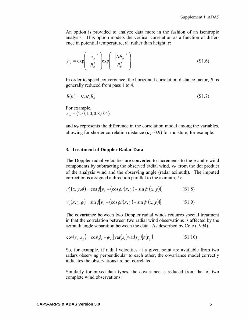
In order to speed convergence, the horizontal correlation distance factor, R, is generally reduced from pass 1 to 4. R(n) = κ nκvRo (S1.7) For example, κ n = 2.0,1.0,0.8,0.4( ) and κv represents the difference in the correlation model among the variables, allowing for shorter correlation distance (κv=0.9) for moisture, for example. 3. Treatment of Doppler Radar Data The Doppler radial velocities are converted to increments to the u and v wind components by subtracting the observed radial wind, vr, from the dot product of the analysis wind and the observing angle (radar azimuth). The imputed correction is assigned a direction parallel to the azimuth, i.e.

( ) ( ) ( )( )[ ]yxvyxuvyxu rj ,sin,coscos,, φφφφ +−=′ (S1.8) ( ) ( ) ( )( )[ ]yxvyxuvyxv rj ,sin,cossin,, φφφφ +−=′ (S1.9)

The covariance between two Doppler radial winds requires special treatment in that the correlation between two radial wind observations is affected by the azimuth angle separation between the data. As described by Cole (1994),

( ) ( ) ( ) ( )[ ] ( )ijjijiji ssss rρφφ varvarcos,cov −= (S1.10) So, for example, if radial velocities at a given point are available from two radars observing perpendicular to each other, the covariance model correctly indicates the observations are not correlated. Similarly for mixed data types, the covariance is reduced from that of two complete wind observations:


Supplement 1: ADAS

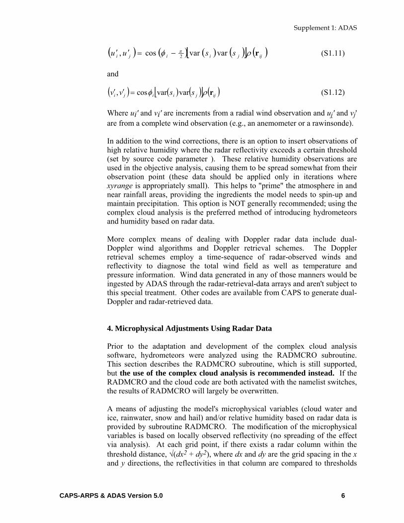
( ) ( ) ( ) ( )[ ] ( )ijjiiji ssuu rρφ π varvarcos, 2−=′′ (S1.11) and ( ) ( ) ( )[ ] ( )ijjiiji ssvv rρφ varvarcos, =′′ (S1.12) Where ui' and vi' are increments from a radial wind observation and uj' and vj' are from a complete wind observation (e.g., an anemometer or a rawinsonde). In addition to the wind corrections, there is an option to insert observations of high relative humidity where the radar reflectivity exceeds a certain threshold (set by source code parameter ). These relative humidity observations are used in the objective analysis, causing them to be spread somewhat from their observation point (these data should be applied only in iterations where xyrange is appropriately small). This helps to "prime" the atmosphere in and near rainfall areas, providing the ingredients the model needs to spin-up and maintain precipitation. This option is NOT generally recommended; using the complex cloud analysis is the preferred method of introducing hydrometeors and humidity based on radar data. More complex means of dealing with Doppler radar data include dual-Doppler wind algorithms and Doppler retrieval schemes. The Doppler retrieval schemes employ a time-sequence of radar-observed winds and reflectivity to diagnose the total wind field as well as temperature and pressure information. Wind data generated in any of those manners would be ingested by ADAS through the radar-retrieval-data arrays and aren't subject to this special treatment. Other codes are available from CAPS to generate dual-Doppler and radar-retrieved data. 4. Microphysical Adjustments Using Radar Data Prior to the adaptation and development of the complex cloud analysis software, hydrometeors were analyzed using the RADMCRO subroutine. This section describes the RADMCRO subroutine, which is still supported, but the use of the complex cloud analysis is recommended instead. If the RADMCRO and the cloud code are both activated with the namelist switches, the results of RADMCRO will largely be overwritten. A means of adjusting the model's microphysical variables (cloud water and ice, rainwater, snow and hail) and/or relative humidity based on radar data is provided by subroutine RADMCRO. The modification of the microphysical variables is based on locally observed reflectivity (no spreading of the effect via analysis). At each grid point, if there exists a radar column within the threshold distance, √(dx2 + dy2), where dx and dy are the grid spacing in the x and y directions, the reflectivities in that column are compared to thresholds


Supplement 1: ADAS

for increasing water vapor, cloud water and/or rainwater (specified in the input file by parameters radqvopt, radqcopt and radqropt , respectively). If the reflectivity is greater than the threshold (refsat or refcld), the water vapor or cloud water variables at the grid point at the level nearest the datum are adjusted. The amount of relative humidity in clouds is specified by input variable rhrad.. The amount of cloud water applied is a fixed value (input parameter cldrad) or while the rain water, snow and hail are determined from a function of the reflectivity. The function is the inverse of that used for plotting reflectivity based on model-produced rainwater, snow and hail. Since this function can produce large amounts of rainwater at high reflectivities, the user is given the option of applying a fractional amount of the rainwater (input parameter cldsetrat) and/or limiting the maximum reflectivity value used in the parameterizing equation (input parameter cldreflim). Finally, since the radar typically only samples a few heights over each horizontal grid column, if there are two observed points within a certain distance (input file parameter dzfill) of each other in the vertical, the microphysical variables in that column are filled-in between those two observations. All microphysical adjustments are not allowed if the grid point is below a specified ceiling (cloud base) limit above ground level. The ceiling limit is specified as a fixed value, ceilmin, or is determined from the LCL of a surface parcel (when ceilopt=2). This is to help prevent ground clutter and/or non-precipitation echoes from creating spurious clouds or rain. One risk of adding rainwater is that the vertical velocities initialized at the location where rainwater is added generally will not support the rainfall, hence the model may create a downdraft (due to the weight of the rainwater) in an area where positive vertical velocity likely exists. It is thought that introducing high relative humidity might help induce condensation processes which in turn would produce latent heat release (adding buoyancy) in addition to the creation of cloud and rainwater. Alternatively, additional buoyancy can be added at the analysis step by means of input parameter radptopt. If the buoyancy balances the additional weight from the cloud and rainwater, the air/water mixture will be initially neutral and initial acceleration determined from other factors. However, the microphysical parameterizations in the model will cause the water itself to fall at its terminal velocity. If no more condensate is produced, the precipitation will entirely fall out. Testing at CAPS is currently exploring various combinations of all these parameters. The best combination may vary depending on whether the model is beginning for a cold start, or updates are being made via an intermittent assimilation cycle.


Supplement 1: ADAS

5. Complex Cloud Analysis A module is included in ADAS to do a complete cloud analysis using surface observations of cloud cover and height, radar and satellite data (Zhang et al. 1998, Brewster 2002). The procedure and code were adapted from the cloud analysis of the Local Analysis and Prediction System (LAPS, Albers et al., 1996) developed at the NOAA Forecast Systems Lab. In ADAS, you can select which of the variables from the cloud analysis contribute to the final output file, and you can control the thresholds applied to radar data. Some of the same concerns about inserting microphysical variables raised in the previous section apply to the variables determined from the cloud analysis. The cloud analysis uses its determination of the cloud type (stratus, stratocumulus or cumulus) to estimate in-cloud vertical velocities. Tests using the ARPS model have shown that vertical velocities determined in this way generally do not last long in the model as the model forcing overwhelms the initial state. Since these initial velocities can trigger condensation in regions of conditionally unstable air masses, there is a risk that the initial vertical velocity can trigger convection, convection that is sometimes spurious due to incorrect cloud type determination. For that reason, use of the cloud vertical velocity for initializing ARPS is not recommended (cldwopt=0 is recommended). The complex cloud analysis is called after the RADMCRO routine and the two work independently, so the user has the option of using cloud water fields from the cloud analysis and rainwater fields from the radar data, for example. Generally the complex cloud analysis is recommended over the RADMCRO. 6. Automated Data Quality Control ADAS includes a few quality-control steps. The surface data are pre-analyzed to compare with each other, and data are rejected if the pre-analysis of neigh-boring observations differs significantly from the observation. Other data are quality-controlled by comparing the observations to the background field in-terpolated to the observation site. Thresholds of allowed differences from the background are set fairly high (in the data error tables provided) to allow for instrument error and errors in representativeness. Representativeness error is especially important in the case of radar data being compared to large-scale gridded forecasts. Statistics are reported in the standard output showing the number and percentage of data points rejected in this manner. Also part of the quality control system is a means to manually exclude data at specified surface stations. This is useful for manual editing and for real-time use when there may be stations that regularly have grossly unrepresentative observations or instrument faults. A file is read containing a list of stations and variable numbers which are excluded from the analysis (they are flagged


Supplement 1: ADAS

as rejected by the quality control). The file is named blacklist.sfc. At this time the blacklist procedure is only implemented for surface data. 7. Incremental Analysis Updating In the standard analysis procedure the analysis updates the background field with information from the observations and the updated field is used as the initial condition for the model run. Alternatively, the background field can be used as the initial field for the model and the increments calculated by the ADAS analysis procedure can be gradually blended into the model solution as the model is running. Providing the increments gradually over time may help some of the unobserved variables adjust while reducing noise in the model forecast. This process, called incremental analysis updating is described in Bloom et al. 1996. Roughly speaking, it can be thought of as a type of nudging. To apply incremental analysis updating, ADAS is run as normal with the increment output switch turned on (incrdmp=1). Then ADAS increment file (named in the ADAS input file) is provided as an input to the ARPS model, and controls for the incrementing time window are specified in the ARPS model input file, arps.input. Storage for the increments is specified in the include file nudging.inc. Before using incremental analysis updating be sure that the grid array dimensions specified in that include file match thedimensions in the dims.inc include file. 8. Steps to Run ADAS • obtain raw data, reformat into LAPS-formatted ASCII files using the FORMAT statements in the source for the various reading routines as a guide, or contact CAPS for examples and documentation of the data file structure. Included in the distribution are programs to process the real-time radar data in both raw, Level-II format (88d2arps_a2) and the Level-III NIDS format (nids2arps). • create background file (generally using EXT2ARPS or an ARPS forecast) • edit adas.inc Specify the size of each of the data categories. Specify dimension as 1 (one) for unused data categories to save memory. Its OK to have extra unused array space, counters keep track of how much data has actually been ingested. • makearps adas • edit arps.input


Supplement 1: ADAS

Edit the namelist variables controlling the ARPS grid, ADAS control, and output naming and formatting. Be sure to specify the proper directory and file names for input of the background field and terrain. The model control variables (dtbig, dtsml, etc, are read-in but are not used). • adas < arps.input >! adas.out • examine output file and ARPS gridded data file using ARPSPLT The gridded-data output file will be named according to the input parameter runname and the history file options. 9. Tips on Setting Parameters and Running ADAS Use the instructions for initializing the ARPS model to initialize the back-ground fields for ADAS. If you're using an ARPS file (from an ARPS fore-cast or output from EXT2ARPS), use initopt=3 and specify the file using inifile and inifmt. When specifying the names of the sources and source error files in the input file, keep in mind that these items are indexed by source, and not by data file. That is the number of data sources need not correspond to the number of files, as some files (such as the surface data files) contain more than one source, and at the same time, it is common to use multiple radar files but they all might come from a single source. It is common to have xyrange decrease gradually with each pass. Execution time will be saved if you introduce dense data (such as radar data) only after first doing iterations to correct the broader scale errors. It is wise to drop coarsely spaced data when xyrange is dictating a correlation range smaller than the average spacing of the data. This prevents the drawing of bullseyes around isolated stations. The inclusion/exclusion of data types is controlled by switches in the input namelists. See the description of usesng, useua, userad, and useret in the table. When the data are very dense, such as a radar data set containing on the order of 104 data points, execution time can become long. Using a cut-off radius can prevent the execution time from becoming excessive. The cut-off radius (distance beyond which a data point has zero influence) is controlled by the input parameter wlim. This parameter is the least value of the correlation function that is allowed, so that a smaller value of wlim will yield a larger cut-off radius. Setting wlim to 10-3 is recommended for very large datasets. The output file indicates what physical distance this limit represents. How well does the analysis fit the data? The fit to the data is largely con-trolled by the expected errors specified for the observations and the back-ground, and to some extent by the correlation ranges used. Smaller xyranges yield analyses that fit the data more closely. If the data are "overfit", the


Supplement 1: ADAS

analysis will have unwanted wiggles in the contours and possibly bullseyes, especially near observation sites. You can see how the analysis is fitting the data by the root-mean-square difference (RMS) statistics printed in the standard output file after each iteration. Regardless of whether xyrange decreases with successive iterations, the RMS statistics should decrease with each pass, and after the final pass the RMS values should approximate the error associated with that observation type. One should note, however, that the actual difference between the interpolated analysis and the observations is likely larger than the printed value -- these show a statistical convergence to the theoretical “truth” rather than toward observations themselves. Also in the RMS table you will see counters of the data. These counters and the diagnostic printing of the reader routines should inform you of the successful ingest of all the data. The reader routines will print warnings if they had to stop reading data because insufficient space was allocated to the data arrays. Generally, ADAS continues processing even if the arrays become full. Recall that data array sizes are specified in adas.inc. You can also examine the fit to the surface data by using ARPSPLT and specifying the observation overlay option (parameter ovrobs =1 in arp-splt.input). Plot the second ARPS vertical level (slice_xy, k=2) and compare the observations to the contours of the analysis. 10. References Albers, S.C., J.A. McGinley, D.A. Birkenhuer, and J.R. Smart, 1996: The

local analysis and Prediction System (LAPS): Analysis of clouds, precipitation and temperature. Wea. and Forecasting, 11, 273-287.

Bloom, S.C., L.L. Takacs, A.M. da Silva, and D. Ledvina, 1996: Data

assimilation using incremental analysis updates. Mon. Wea. Rev., 124, 1256-1271.

Bratseth, A.M., 1986: Statistical interpolation by means of successive correc-

tions. Tellus, 38A, 439-447. Brewster, K., 2002: Recent advances in the diabatic initialization of a non-

hydrostatic numerical model. Preprints, 21st Conf. on Severe Local Storms, and Preprints, 15th Conf. Num. Wea. Pred. and 19th Conf. Wea. Anal. Forecasting, Amer. Meteor. Soc., J51-J54.

Cole, R.E. and F.W. Wilson, 1995: ITWS Gridded Wind Product, Preprints,

6th Conf. on Aviation Wetaher Systems, AMS, Boston. Lorenc, A.C., R.S. Bell and B. MacPherson, 1991: The Meteorological Office

analysis correction data assimilation scheme. Quart. J. Roy. Meteor. Soc., 117, 59-89.


Supplement 1: ADAS

Sashegyi, K.D., D.E. Harms, R.V. Madala, S. Raman, 1993: Application of

the Bratseth scheme for the analysis of GALE data using a mesoscale model. Mon. Wea. Rev., 121, 2331-2350.

Zhang, J., F. Carr, and K. Brewster, 1998: ADAS cloud analysis. Preprints,

12th Conf. on Num. Wea. Prediction, Phoenix, AZ, AMS, Boston, 185-188.


Supplement 1: ADAS

Analysis Increment Output Options (&incr_out)

Parameter Definition/Purpose Options/Suggested Values

incrdmp

Switch to output analysis increments in a file for reading by ARPS if analysis increment updating is desired.

0: no file is written 1: binary format file 3: HDF format file

incrhdfcompr Level of compression in HDF file.

0: no compression 1-3: increasing compression level

incdmpf

Name of increment output file.

Full name of file

uincdmp vincdmp wincdmp pincdmp ptincdmp qvincdmp qcincdmp qrincdmp qiincdmp

qsincrdmp qhincdmp

Switches to output analysis increments for individual variables. u,v,w,p,pt,qv,qc,qr,qi,qs,qh

0: increments not written 1: binary format file 3: HDF format file

ADAS Constants

(&adas_const) Parameter Definition/Purpose Options/Suggested Values

npass

Number of analysis passes or iterations of the Bratseth or Barnes schemes.

Typical: 3 or 4 passes

sprdist Super-ob distance (m). Surface observations closer than sprdist will be combined into a single-superob before beginning the analysis.

Scale (dx) dependent, approximately 15000 m. (15 km)


Supplement 1: ADAS

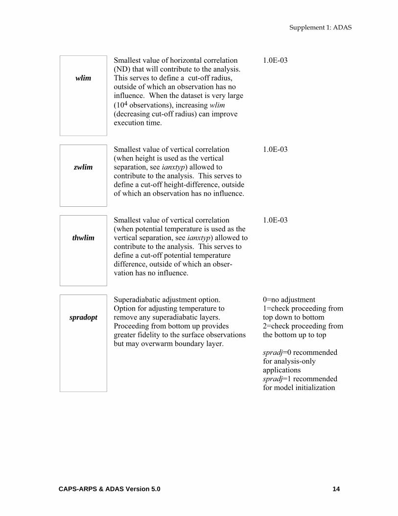
wlim

Smallest value of horizontal correlation (ND) that will contribute to the analysis. This serves to define a cut-off radius, outside of which an observation has no influence. When the dataset is very large (104 observations), increasing wlim (decreasing cut-off radius) can improve execution time.

1.0E-03

zwlim

Smallest value of vertical correlation (when height is used as the vertical separation, see ianxtyp) allowed to contribute to the analysis. This serves to define a cut-off height-difference, outside of which an observation has no influence.

1.0E-03

thwlim

Smallest value of vertical correlation (when potential temperature is used as the vertical separation, see ianxtyp) allowed to contribute to the analysis. This serves to define a cut-off potential temperature difference, outside of which an obser-vation has no influence.

1.0E-03

spradopt

Superadiabatic adjustment option. Option for adjusting temperature to remove any superadiabatic layers. Proceeding from bottom up provides greater fidelity to the surface observations but may overwarm boundary layer.

0=no adjustment 1=check proceeding from top down to bottom 2=check proceeding from the bottom up to top spradj=0 recommended for analysis-only applications spradj=1 recommended for model initialization


Supplement 1: ADAS

ccatopt

Option to adjust horizontal correlations for differences in precipitation categories.

0 : Isotropic correlation functions used. 1 : Correlation is reduced between dry areas and areas of precipitation, especially where the cumulus parameterization is activated. ccatopt=1 recommended when ADAS is run using a background field from an ARPS run including cumulus parameterization.

ADAS Adjustment Options

(&adjust)

hydradj

Superadiabatic adjustment option. Option for adjusting pressure to balance temperature field to create a balanced state for model initialization. Formerly known as boycor.

0=no pressure adjust. 1=use model eqs, beginning at bottom 2=use model eqs, beginning at top 3=hydrostatic pressure, beginning at bottom hydradj=0 recommended

wndadj

Option for adjusting wind field after horizontal winds have been analyzed.

0=no wind adjust. 1=w is set so wcont=0 no changes to u, v 2=w is set using horiz divergence and O'Brien method for top bc see obropt 3=as in 2, but u,v are relaxed to create zero 3-D divergence windadj=2 recommended


Supplement 1: ADAS

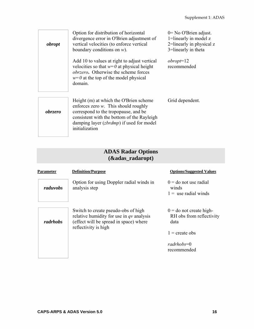
obropt

Option for distribution of horizontal divergence error in O'Brien adjustment of vertical velocities (to enforce vertical boundary conditions on w). Add 10 to values at right to adjust vertical velocities so that w=0 at physical height obrzero. Otherwise the scheme forces w=0 at the top of the model physical domain.

0= No O'Brien adjust. 1=linearly in model z 2=linearly in physical z 3=linearly in theta obropt=12 recommended

obrzero

Height (m) at which the O'Brien scheme enforces zero w. This should roughly correspond to the tropopause, and be consistent with the bottom of the Rayleigh damping layer (zbrdmp) if used for model initialization

Grid dependent.

ADAS Radar Options (&adas_radaropt)


raduvobs

Option for using Doppler radial winds in analysis step

0 = do not use radial winds 1 = use radial winds

radrhobs

Switch to create pseudo-obs of high relative humidity for use in qv analysis (effect will be spread in space) where reflectivity is high

0 = do not create high- RH obs from reflectivity data 1 = create obs radrhobs=0 recommended


Supplement 1: ADAS

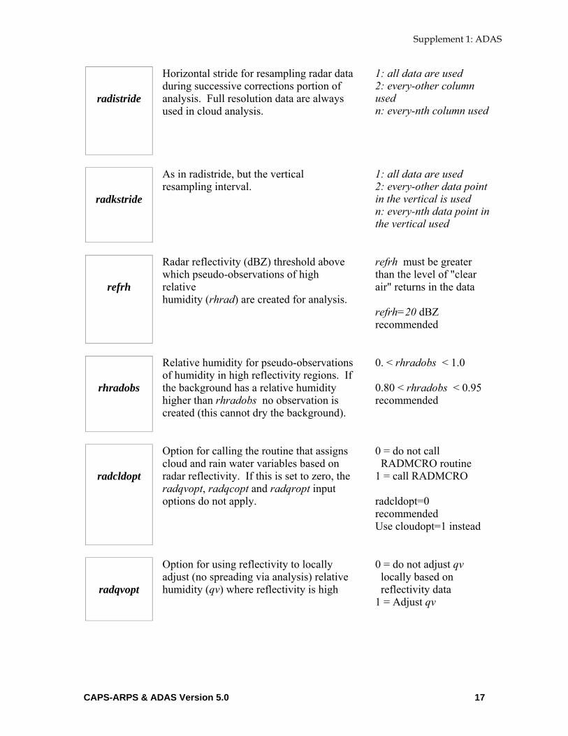
radistride

Horizontal stride for resampling radar data during successive corrections portion of analysis. Full resolution data are always used in cloud analysis.

1: all data are used 2: every-other column used n: every-nth column used

radkstride

As in radistride, but the vertical resampling interval.

1: all data are used 2: every-other data point in the vertical is used n: every-nth data point in the vertical used

refrh

Radar reflectivity (dBZ) threshold above which pseudo-observations of high relative humidity (rhrad) are created for analysis.

refrh must be greater than the level of "clear air" returns in the data refrh=20 dBZ recommended

rhradobs

Relative humidity for pseudo-observations of humidity in high reflectivity regions. If the background has a relative humidity higher than rhradobs no observation is created (this cannot dry the background).

0. < rhradobs < 1.0 0.80 < rhradobs < 0.95 recommended

radcldopt

Option for calling the routine that assigns cloud and rain water variables based on radar reflectivity. If this is set to zero, the radqvopt, radqcopt and radqropt input options do not apply.

0 = do not call RADMCRO routine 1 = call RADMCRO radcldopt=0 recommended Use cloudopt=1 instead

radqvopt

Option for using reflectivity to locally adjust (no spreading via analysis) relative humidity (qv) where reflectivity is high

0 = do not adjust qv locally based on reflectivity data 1 = Adjust qv


Supplement 1: ADAS

radqcopt

Option for using reflectivity to locally adjust (no spreading via analysis) cloud water (qc) where reflectivity is high

0 = do not adjust qc locally based on reflectivity data 1 = adjust qc using fixed cloud water mixing ratio 2 = adjust qc using cloud water mixing ratio that is a function of observed reflectivity.

radqropt

Option for using reflectivity to locally adjust (no spreading via analysis) rainwater (qr) where reflectivity is high

0 = do not adjust qr locally based from reflectivity data 1 = adjust qr using rain water mixing ratio that is a function of observed reflectivity.

radptopt

Option for adjusting potential temperature to create a net zero buoyancy change in combination with the weight added by increasing qr and qc and/or the weight removed by increasing qv.

0 = do not adjust potential temperature 1 = adjust temperature for rain and cloud water only 2 = adjust temperature for humidity adjustment only 3 = adjust for all changes to qr, qc, and qv

refsat Reflectivity threshold (dBZ) to use in local "saturation" adjustment.

10. < refsat < 35. dBZ recommend

rhrad

Relative humidity (0.0-1.0) to apply in local saturation adjustment. No adjustment is made if background humidity is higher.

0.80 < rhrad < 1.0 recommended


Supplement 1: ADAS

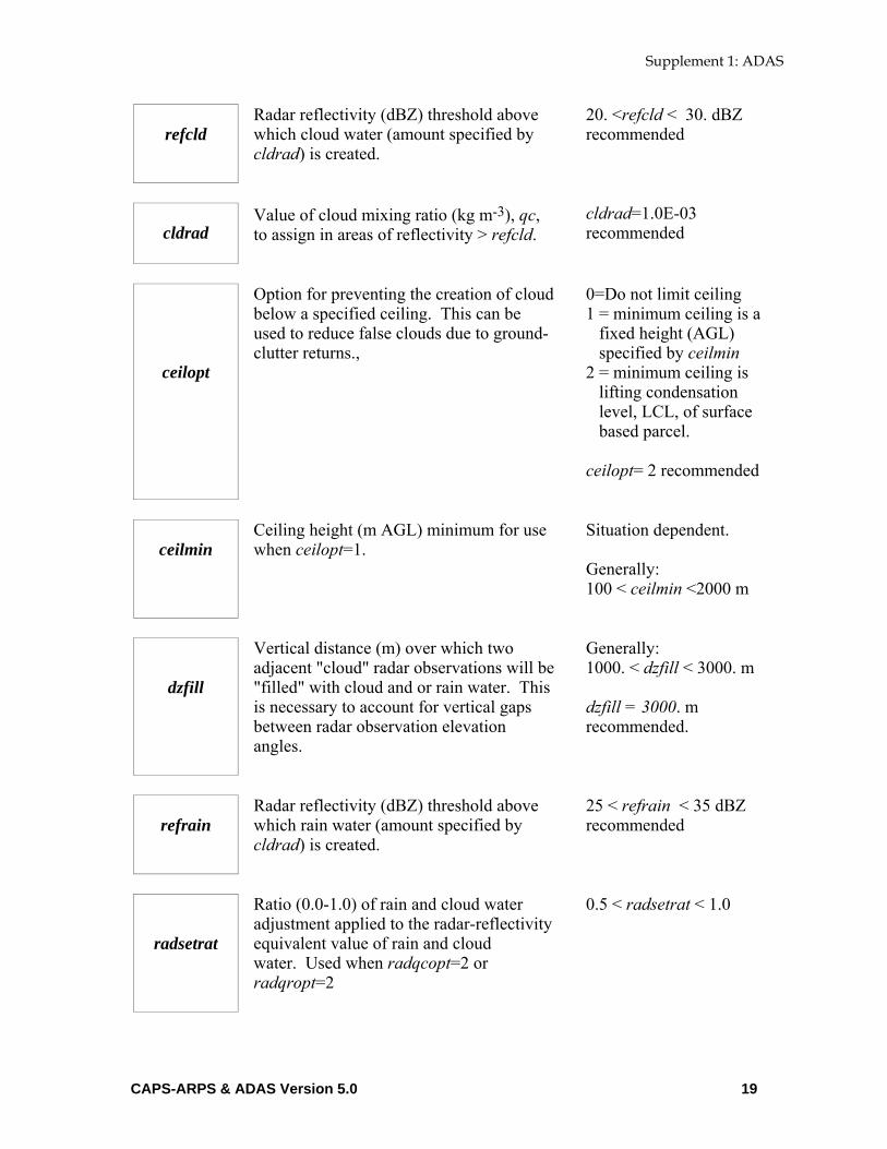
refcld

Radar reflectivity (dBZ) threshold above which cloud water (amount specified by cldrad) is created.

20. <refcld < 30. dBZ recommended

cldrad Value of cloud mixing ratio (kg m-3), qc, to assign in areas of reflectivity > refcld.

cldrad=1.0E-03 recommended

ceilopt

Option for preventing the creation of cloud below a specified ceiling. This can be used to reduce false clouds due to ground-clutter returns.,

0=Do not limit ceiling 1 = minimum ceiling is a fixed height (AGL) specified by ceilmin 2 = minimum ceiling is lifting condensation level, LCL, of surface based parcel. ceilopt= 2 recommended

ceilmin Ceiling height (m AGL) minimum for use when ceilopt=1.

Situation dependent. Generally: 100 < ceilmin <2000 m

dzfill

Vertical distance (m) over which two adjacent "cloud" radar observations will be "filled" with cloud and or rain water. This is necessary to account for vertical gaps between radar observation elevation angles.

Generally: 1000. < dzfill < 3000. m dzfill = 3000. m recommended.

refrain Radar reflectivity (dBZ) threshold above which rain water (amount specified by cldrad) is created.

25 < refrain < 35 dBZ recommended

radsetrat

Ratio (0.0-1.0) of rain and cloud water adjustment applied to the radar-reflectivity equivalent value of rain and cloud water. Used when radqcopt=2 or radqropt=2

0.5 < radsetrat < 1.0


Supplement 1: ADAS

radreflim

Upper bound on reflectivity (dBZ) to use in calculating the rain and cloud water when radqcopt=2 or radqropt=2.

40 < radreflim < 50 dBZ

radptgain Multiplier to apply to potential temperature perturbation calculated to balance water loading. radptgain greater than unity will result in positive buoyancy where there are clouds.

1.0 < radptgain < 2.0

ADAS Cloud Options (&adas_cloudopt)


cloudopt

Option for calling the ADAS complex cloud analysis. The routine uses all available data sources to assign cloud coverage. Cloud microphysical variables can be assigned in the model based on the final cloud analysis (see options, below). The cloud analysis is Jian Zhang's modification of the FSL LAPS cloud analysis.

0 = do not run the complex cloud analysis. 1 = run the complex cloud analysis

clddiag Option for printing voluminous diagnostics related to the cloud analysis.

0 = do not print the extra diagnostics. 1 = print diagnostics.

cld_files

Option to output files containing intermediate cloud fields (cloud base, cloud top, ceiling and column VIL). This information is not included in the standard ADAS/ARPS grid file.

0 = do not write cloud files. 1 = write cloud files.

range_cld Horizontal distance (m) for use in the horizontal spreading of analyzed clouds from point observations.

range_cld=104-105 m (10-100 km) recommended


Supplement 1: ADAS

refthr1

Reflectivity threshold (dBZ) for assigning cloud based on radar data below hgtrefthr. Generally, refthr1 is set to eliminate false ground clutter

refthr1=25. recommended

refthr2

Reflectivity threshold (dBZ) for assigning cloud based on radar data above hgtrefthr. Generally, refthr2 is set to eliminate insect or non-precipitation scatter returns.

refthr2=20. recommended

hgtrefthr

Height (m AGL) of transition from using refthr1 to using refthr2.

hgtrefthr=2000. m recommended

thresh _cvr

Threshold of sky cover to set cloud water and vertical velocity. Below thresh_cvr no adjustments to those variables are made.

0.0 < thresh_cvr <1.0 0.45<thresh_cvr<0.65 recommended

bgqcopt Option for using relative humidity in the background field to create cloud water (qc) within the cloud analysis. Note that the ARPS output file cloud field is not changed unless the cldqcopt option (below) is set to 1.

0 = do not adjust qc locally based on background relative humidity. 1 = adjust qv

cldqvopt Option for using results of the cloud analysis to locally adjust (no spreading via analysis) relative humidity (qv).

0 = do not adjust qv locally based on cloud analysis. 1 = adjust qv

rh_thr1

Lower end of RH for the linear cloud-cover-to-RH relationship.

0.0 < rh_thr1 < rh_trh2 rh_thr1=0..50 recommended

cvr2rh _thr1

Lower end of cloud-cover for the linear cloud-cover-to-RH relationship.

0.0 < cvr2rh_thr1 <1.0 cvr2rh_thr1=0..20 recommended


Supplement 1: ADAS

rh_thr2

Upper end of RH for the linear cloud-cover-to-RH relationship.

rh_thr1 < rh_thr2 <1.0 rh_thr2=0..98 recommended

cvr2rh _thr1

Upper end of cloud-cover for the linear cloud-cover-to-RH relationship.

0.0 < cvr2rh_thr2<1.0 cvr2rh_thr2=0..70 recommended

cldqcopt

Option for using results of the cloud analysis to locally adjust (no spreading via analysis) cloud water (qc). Where temperature is cold enough cloud ice (qi) can be affected

0 = do not adjust qc locally based on cloud analysis 1 = adjust qc

qvslimit 2_qc

Upper limit for analyzed qc. qc < qvslimit_2_qc * qvsat, where qvsat is saturation specific humidity

0.0 < qvslimit_2_qc <5.0 qvslimit_2_qc=1.0 recommended

cldqropt Option for using results of the cloud analysis to locally adjust (no spreading via analysis) rainwater (qr).

0 = do not adjust qr locally based on cloud analysis. 1 = adjust qr

qrlimit

Upper limit on analyzed qr (kg/kg).

0.0 < qrlimit < 0.01 qrlimit=0.005 recommended

frac_qr _2_qc

Fraction of qr converted into qc.

0.0 < frac_qr_2_qc <1.0 frac_qr_2_qc=0.0 recommended


Supplement 1: ADAS

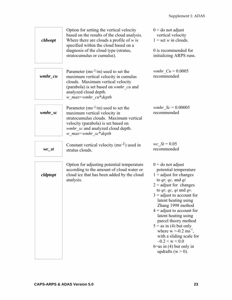
cldwopt

Option for setting the vertical velocity based on the results of the cloud analysis. Where there are clouds a profile of w is specified within the cloud based on a diagnosis of the cloud type (stratus, stratocumulus or cumulus).

0 = do not adjust vertical velocity 1 = set w in clouds. 0 is recommended for initializing ARPS runs.

wmhr_cu

Parameter (ms-1/m) used to set the maximum vertical velocity in cumulus clouds. Maximum vertical velocity (parabola) is set based on wmhr_cu and analyzed cloud depth. w_max=wmhr_cu*depth

wmhr_Cu = 0.0005 recommended

wmhr_sc

Parameter (ms-1/m) used to set the maximum vertical velocity in stratocumulus clouds. Maximum vertical velocity (parabola) is set based on wmhr_sc and analyzed cloud depth. w_max=wmhr_sc*depth

wmhr_Sc = 0.00005 recommended

wc_st

Constant vertical velocity (ms-1) used in stratus clouds.

wc_St = 0.05 recommended

cldptopt

Option for adjusting potential temperature according to the amount of cloud water or cloud ice that has been added by the cloud analysis.

0 = do not adjust potential temperature 1 = adjust for changes to qr, qc, and qi 2 = adjust for changes to qr, qc, qi and qv. 3 = adjust to account for

latent heating using Zhang 1998 method

4 = adjust to account for latent heating using parcel theory method

5 = as in (4) but only where w >-0.2 ms-1, with a sliding scale for –0.2 < w < 0.0

6=as in (4) but only in updrafts (w > 0).


Supplement 1: ADAS

frac_qw

_2_pt

Gain factor for the potential temperature adjustment used to preserve neutral buoyancy where water is analyzed. Used only when cldptopt=1 or 2.

0.0 < frac_qw_2_pt <5.0 frac_qw_2_pt=1.0 recommended

frac_qc _2_lh

Gain factor for the potential temperature adjustment from latent heating. Used only when cldptopt=3.

0.0 < frac_qc_2_lh<5.0 frac_qc_2_lh=1.0 recommended

max_lh _2_pt

Maximum potential temperature adjustment (K) based on latent heating. Used only when cldptopt=3.

0.0 < max_lh_2_pt <15. max_lh_2_pt=8.0 recommended

smth_opt Option to apply smoothing on the analyzed moisture and in-cloud w.

0 = do not smooth 1 = Apply 2-D smoothing 2 = Apply 3-D smoothing

nirfiles

Number of IR satellite data files.

Integer

ir_fname Name of remapped IR satellite data file. Set to 'NULL' or a dummy filename if no IR data are available.

Character string(s) in quotes.

ircalname Name calibration data file to match each IR file named in ir_fname array.


nvisfiles

Number of visible satellite data files.

Integer

vis_ fname

Name of remapped visible satellite data file. Set to 'NULL' or a dummy filename if no visible data are available.



Supplement 1: ADAS

viscal name

Name calibration data file to match each visible file named in vis_fname array.


ADAS Analysis Types (&adas_typ)


ianxtyp (ipass)

Type of analysis for each pass.

11=Barnes, height vert 12=Barnes, theta vert 21=Bratseth, height vert 22=Bratseth, theta vert Default: 21

ADAS Range (&adas_range)


sfcqcrng

Scale distance (m) for the Barnes weighting function used in the quality control of surface data.

Data spacing dependent. Generally: 30.E03 < sfcqcrng < 100.E03 m

xyrange (ipass)

Horizontal scale for the correlation function in the analysis. See body of this document for guidelines on setting the correlation range.

Depends on data density and data switches. Example: xyrange(1)=100.E03 xyrange(2)=60.E03 xyrange(3)=5.E03


Supplement 1: ADAS

ADAS Kappa Variable (&adas_kpvar)


kpvar (ivar)

Scaling factor (ND) which multiplies xyrange making the scale different for each variable. One for each variable, where variable 1: u wind component variable 2: v wind component variable 3: pressure variable 4: potential temperature variable 5: humidity

Generally: 0.5 < kpvar < 2.0 Default: kpvar(1)=0.9 kpvar(2)=0.9 kpvar(3)=1.0 kpvar(4)=1.0 kpvar(5)=0.9

ADAS Z-range (&adas_zrange)


zrange (ipass)

Range (m) for vertical correlation model when analysis using height separation is used. A value is specified for each pass even though the options may be set to use theta in the vertical.

Typical: 500. < zrange < 1800.

ADAS Theta-range (&adas_thrange)



Supplement 1: ADAS

thrange (ipass)

Range (K) for vertical correlation model when analysis using potential temperature separation is used. A value is specified for each pass even though the options may be set to use height in the vertical.

Typical: thrange(ipass)= 5 K.

ADAS Background Error File (&adas_backerf)


backerrfil

Name of background error file character*132

Typical: backerrfil= 'ruc3herr.adastab'

ADAS Single-Level Data Specifications (&adas_sng)


nsngfil

Number of single-level data files. Single level data include surface data and pilot report data.

Data dependent. Typical: 1 or more nsngfil ≤ mx_sng_file (mx_sng_file is set in adas.inc)

sngfname (ifile)

Name of single-level data file Repeat for nsngfils. character*132

Typical: sngfname(1)= 'jun08/951591500.lso'

sngtimchk

(ifile)

Name of data file used for time consistency check of respective sngfname data. Dataset of the same type from a previous time period. Specify a dummy filename if no such data are available. character*132

Typical: sngtimchk(1)= 'jun08/951591400.lso'


Supplement 1: ADAS

srcsng (isrc)

Following are repeated for each data source in the single-level data file(s). Note that a single-level file can contain one or more sources. Largest index, isrc, used must be less than or equal to nsrc_sng (nsrc_sng is set in adas.inc). Name of data source. These must match the source name(s) in the data file(s). character*8

Typical: srcsng(1)='SA'

sngerrfil (isrc)

Name of file containing error specification table for each source. character*132

Typical: sngerrfil(1)= 'saoerr.adastab'

iusesng (isrc, ipass)

Integer switch indicating whether the data source should be used on each pass. A switch is required for each pass, i.e. iusesng(1,1), iusesng(1,2)...

0: Do not use data from this source on this pass. 1: use data Example: iusesng(1,1)=0, iusesng(1,2)=1, iusesng(1,3)=0

ADAS Multiple-Level Data Specifications (&adas_ua)


nuafil

Number of multiple-level data files. Multiple level data include radiosonde data and profiler data.

Data dependent. Typical: 1 or more nuafil ≤ mx_ua_file (mx_ua_file is set in adas.inc)


Supplement 1: ADAS

uafname

(ifile)

Name of multiple-level data file Repeat for nuafils. character*132

Typical: uafname(1)= 'jun08/951591500.snd'

srcua (isrc)

Following are repeated for each data source in the multiple-level data file(s). Note that a multiple-level file usually contains one source, but more than one file may have the same source. Largest index, isrc, used must be less than or equal to nsrc_ua. (nsrc_ua is set in adas.inc). Name of data source. character*8

Typical: srcua(1)=''NWS RAOB'

uaerrfil (isrc)


Typical: uaerrfil(1)= 'snderr.adastab'

iuseua (isrc, ipass)

Integer switch indicating whether the data source should be used on each pass. A switch is required for each pass, i.e. iuseua(1,1), iuseua(1,2)...

0: Do not use data from this source on this pass. 1: use data Data dependent Example: iuseua(1,1)=1, iuseua(1,2)=0, iuseua(1,3)=0

ADAS Radar Data Specifications (&adas_radar)



Supplement 1: ADAS

nradfil

Number of remapped radar data files. Remapped radar data files are created by mapping raw data onto a regular grid, which need not match the final analysis grid.

Data dependent. Typical: 0 or more nradffl ≤ mx_rad_file (mx_rad_file is set in adas.inc)

radfname (ifile)

Name of radar data file(s) Repeat for nradfils. character*132

Typical: radfname(1)= 'KTLX.950507.1756'

srcrad (isrc)

Following are repeated for each data source in the radar data file(s). Note: that a radar data file contains one source, but more than one file may have the same source. Largest index, isrc, used must be less than or equal to nsrc_rad (nsrc_rad is set in adas.inc). Name of data source. character*8

Typical: srcrad(1)='88D-AII' srcrad(2)=’NIDS’

raderrfil (isrc)


Typical: raderrfil(1)= 'data/adas/88derr.adastab' raderrfil(2)= 'data/adas/nidserr.adastab'

iuserad (isrc, ipass)

Integer switch indicating whether the radar data source should be used on each pass. A switch is required for each pass, i.e. iuserad(1,1), iuserad(1,2)...

0: Do not use data from this source on this pass. 1: use data Data dependent Example: iuserad(1,1)=0, iuserad(1,2)=0, iuserad(1,3)=1


Supplement 1: ADAS

ADAS Retrieved Radar Data Specifications (&adas_retrieval)


nretfil

Number of radar retrieved data files. Retrieved data files are created by separate radar retrieval programs.

Data dependent. Typical: 0 or more nretfil ≤ mx_ret_file (mx_ret_file is set in adas.inc)

retfname (ifile)

Name of radar retrieval data file Repeat for nretfils. character*132

Typical: retfname(1)= 'KTLXret.960526.1700'

srcret (isrc)

Following are repeated for each data source in the retrieval data file(s). Note that a retrieval data file contains one source, but more than one file may have the same source. Largest index, isrc, used must be less than or equal to nsrc_ua. (nsrc_ret is set in adas.inc). Name of data source. character*8

Typical: srcret(1)='88D-RET'

reterrfil (isrc)


Typical: reterrfil(1)= '88dreterr.adastab'


Supplement 1: ADAS

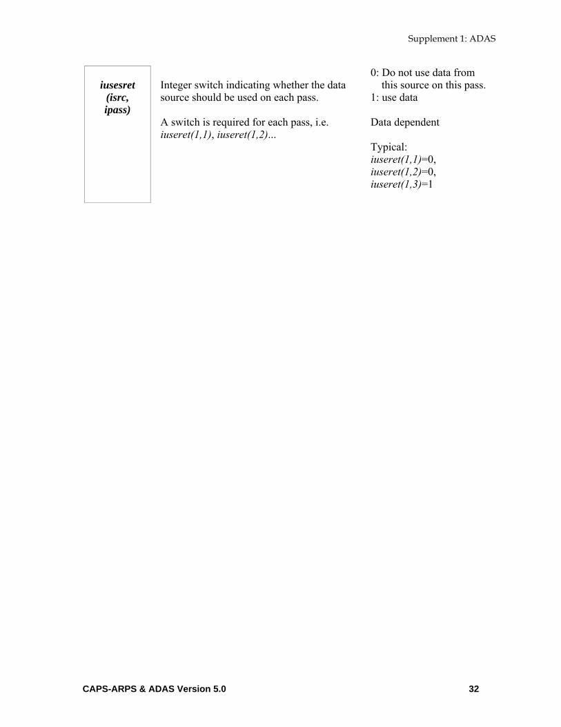
iusesret

(isrc, ipass)

Integer switch indicating whether the data source should be used on each pass. A switch is required for each pass, i.e. iuseret(1,1), iuseret(1,2)...

0: Do not use data from this source on this pass. 1: use data Data dependent Typical: iuseret(1,1)=0, iuseret(1,2)=0, iuseret(1,3)=1


Documents

S-1 3-D Analysis with ARPS Data Assimilation System ... - CAPS